Theoretically Improving Graph Neural Networks via Anonymous Walk Graph KernelsConference: Proceedings of the Web Conference 2021; April 19–23, 2021; Ljubljana, SloveniaProceedings of the Web Conference 2021 (WWW ’21), April 19–23, 2021, Ljubljana, SloveniaDOI: 10.1145/3442381.3449951ISBN: 978-1-4503-8312-7/21/04CCS: Networks Network structureCCS: Information systems Collaborative and social computing systems and tools
Abstract.
Graph neural networks (GNNs) have achieved tremendous success in graph mining. However, the inability of GNNs to model substructures in graphs remains a significant drawback. Specifically, message-passing GNNs (MPGNNs), as the prevailing type of GNNs, have been theoretically shown unable to distinguish, detect or count many graph substructures. While efforts have been paid to complement the inability, existing works either rely on pre-defined substructure sets, thus being less flexible, or are lacking in theoretical insights. In this paper, we propose GSKN11 1 Our codes are available at https://github.com/YimiAChack/GSKN, a GNN model with a theoretically stronger ability to distinguish graph structures. Specifically, we design GSKN based on anonymous walks (AWs), flexible substructure units, and derive it upon feature mappings of graph kernels (GKs). We theoretically show that GSKN provably extends the 1-WL test, and hence the maximally powerful MPGNNs from both graph-level and node-level viewpoints. Correspondingly, various experiments are leveraged to evaluate GSKN, where GSKN outperforms a wide range of baselines, endorsing the analysis.
Keywords:
Graph Convolutional Network, Structural Patterns, Graph Kernels1. Introduction
Graph Neural Networks (GNNs) (Wu et al. 2020; Xu et al. 2018) have achieved tremendous success in mining information networks, such as social networks, knowledge graphs, and biochemical networks (Duvenaud et al. 2015; Niepert et al. 2016; Kipf and Welling 2017; Hamilton et al. 2017). Underlying most widely studied GNNs (Veličković et al. 2017; Kipf and Welling 2017; Hamilton et al. 2017) lies the mechanism of message passing (Gilmer et al. 2017; Bayati and Montanari 2011), or neighborhood aggregation (Xu et al. 2018), where the representations for each node are updated by aggregating information from their neighbors. It is such a mechanism that enables efficient recursive computation of graph and node representations and promotes its tremendous success.
However, message passing and the resultant message passing GNNs (MPGNNs), as the majority of GNNs, bear inherent drawbacks in capturing substructures of graphs. For example, (Xu et al. 2018; Morris et al. 2019) show that the capability of distinguishing different graphs of MPGNNs is upper-bounded by the 1-Weisfeiler-Lehman Isomorphism Test (1-WL Test), which is known unable to distinguish many common substructures (examples in (Sato 2020)). In addition, (Chen et al. 2020a; Arvind et al. 2020) show that MPGNNs are unable to count or detect substructures with 3 or more nodes. Both theoretical results uncover crucial limitations of MPGNNs, as graph substructures are widely recognized as indicative in various complex networks. For example, cliques, or community structures are common patterns in social networks (Granovetter 1973), and rings serve as indicators on functional groups in molecular chemistry (Liu et al. 2017), etc. Whether and how we can extend MPGNNs to account for substructures in complex graphs is thus an important open problem, posed by the contrast between the significance of substructures, and the inability of MPGNNs to model them.
There have been several attempts aiming to improve MPGNNs for better modeling of substructures (Bouritsas et al. 2020; Lee et al. 2019; Long et al. 2020; Jin et al. 2020). However, (Lee et al. 2019; Bouritsas et al. 2020) design their solutions based on pre-defined substructure patterns, namely motifs and graphlets, which should be fixed prior to model learning. The reliance on fixed sets of substructures leads to a lack of versatility when applied to diverse real-world networks, each of which may be characterized by different substructures. On the other hand, (Jin et al. 2020; Long et al. 2019) eliminate the reliance on pre-selected substructures through a flexible substructure pattern named anonymous walks (AW) (Micali and Zhu 2016). However, their solutions are largely empirical, in that they fail to compare their solutions against MPGNNs in a principled theoretical manner. As we would like to preserve the versatility and independence from pre-selection, studying AW based GNNs in a theoretically principled manner becomes our primary focus.
We resort to a parallel line of work on graph mining, namely Graph Kernels (GKs). Graph kernels are classical methods that measure similarities between pairwise substructures, nodes, or graphs and hence enable graph clustering, comparison, and classification (Narayanan et al. 2017; Shervashidze et al. 2011; Zhang et al. 2018). We consider graph kernels appropriate for our problem for three reasons. First, graph kernels inherently involve comparisons between substructures, such as subtrees (Shervashidze et al. 2011), graphlets (Shervashidze et al. 2009) and random walks (Kang et al. 2012), making it natural for us to incorporate and analyze AW in the framework. In addition, connections between GKs and GNNs have been well-identified (Lei et al. 2017; Chen et al. 2020b; Du et al. 2019), making it easier to adapt the theory on graph kernels to design and analyze GNNs. Finally, although graph kernels on AW have been proposed by AWE (Ivanov and Burnaev 2018), both the relationship between AWE and GNNs, and analyses on AWE remain elusive. We, therefore, consider GKs as instrumental tools in theoretically bridging AW to GNNs.
In this paper, we propose the Graph Structural Kernel Network (GSKN), a GNN model derived from GKs that incorporates AWs and provably extends MPGNNs and the 1-WL test in terms of distinguishing graph structures. Specifically, we first design the anonymous walk graph kernel (AWGK), and derive the its GNN architecture to compute its kernel mapping. We build GSKN by combining the kernel mapping of AWGK with existing graph kernel mappings. We further analyze theoretically the ability of GSKN to distinguish graph structures from both graph-level and node-level viewpoints, on both of which GSKN is provably more powerful than MPGNNs and the 1-WL test. Correspondingly, we carry out extensive experiments on both graph and node classification tasks, GSKN outperforms various strong baselines in all scenarios, which coincides with the theoretical analysis and endorses its versatility.
We summarize our contributions as follows:
- •
We propose GSKN, a GNN model based on GKs and anonymous walks that complements the inability to model substructures of MPGNNs in a theoretically principled manner.
- •
We design the anonymous walk graph kernel (AWGK) and derive the corresponding GNN architecture to compute its kernel mapping. We further build GSKN by flexibly combining AWGK with existing graph kernel mappings.
- •
We theoretically show that GSKN possesses a stronger ability to distinguish graph structures from both graph-level and node-level viewpoints.
- •
Graph and node classification on synthetic and real-world datasets are carried out, where GSKN outperforms various strong baselines, coinciding with the theoretical analysis.
2. Related Work
2.1. Graph Neural Networks (GNNs)
Yet GNNs were proposed in relatively early ages (Scarselli et al. 2008), only in recent years did we observe their tremendous success (Hamilton et al. 2017; Veličković et al. 2017). One important reason underlying the popularity is the simplification from spectral methods (Chung and Graham 1997) to localized models (Defferrard et al. 2016; Kipf and Welling 2017; Wu et al. 2019), which connects GNNs to message passing (Gilmer et al. 2017; Bayati and Montanari 2011), or neighborhood aggregation (Xu et al. 2018) and significantly promotes the efficiency of GNNs. Consequently, GNNs proposed henceforth largely belong to the category of message-passing GNNs (MPGNNs) (Chen et al. 2020a; Veličković et al. 2017).
However, MPGNNs bear drawbacks in their ability to model substructures in graphs. For example, it is shown by (Morris et al. 2019; Xu et al. 2018) that the ability of MPGNNs to distinguish graphs is upper bounded by the 1-Weisfeiler-Lehman Isomorphism Test (1-WL Test). 1-WL Test is known to be blind to regular graphs, and analysis by (Sato 2020) shows that numerous pairwise graphs besides regular graphs can also fool the 1-WL Test, and hence MPGNNs. As another example, (Chen et al. 2020a; Arvind et al. 2020) show that MPGNNs are neither able to count subgraph isomorphisms for patterns with more than 3 nodes, nor able to detect any subgraphs other than forests of stars. These analyses point out the inherent limitations of MPGNNs on tackling graph substructures.
2.2. Substructures in Graph Mining
Substructures have been identified as important indicators in graph mining since (Granovetter 1973), who pointed out the significance of triads in social networks. Later works focus on more diverse sets of substructures, such as motifs (Milo et al. 2002), i.e. over-represented subgraph patterns, and graphlets (Pržulj 2007), i.e. induced subgraph patterns. These substructures have proven to be indicative in analyzing numerous types of graphs, including biochemical networks (Pržulj 2007), social networks (Juszczyszyn et al. 2008; Li et al. 2017; Paranjape et al. 2017) and even semantic segmentation (Zhang et al. 2013).
The importance of substructures motivates researchers to seek solutions that complement MPGNNs with the awareness of substructures. One line of works aims to leverage network motifs and graphlets (Lee et al. 2019; Bouritsas et al. 2020) to build substructure-aware GNNs. However, both of them rely on fixed sets of motifs and graphlets that need to be selected prior to model learning. Since real-world networks are diverse and may be characterized by varying types of substructures, the reliance on pre-selection significantly limits their applications in practice. Another line of works resort to a more flexible substructure unit called anonymous walks (AW) (Jin et al. 2020; Long et al. 2020) which do not require pre-selection, and build GNN models with impressive empirical results. However, one common drawback of them is that they fail to demonstrate their solutions compared to MPGNNs in a theoretically principled manner.
2.3. Graph Kernels (GKs)
Kernel methods have been widely studied and applied in general machine learning (Shawe-Taylor et al. 2004). Kernel methods evaluate pairwise similarities between data samples through kernel functions, during which the data samples are implicitly projected onto higher dimensional spaces (called the Reproducing Kernel Hilbert Space, RKHS) and thus endowed with richer features to facilitate classification.
Kernel methods on graphs, namely Graph Kernels (GK) evaluate pairwise similarity between nodes or graphs by decomposing them into basic structural units, characteristic choices of which include random walks (Kang et al. 2012), subtrees (Shervashidze et al. 2011), shortest paths (Borgwardt and Kriegel 2005), graphlets (Shervashidze et al. 2009), and also AW (Ivanov and Burnaev 2018). Such decomposition, provides principled manners to analyze the ability of GKs to express graph structures (Kriege et al. 2018; Chen et al. 2020b; Gärtner et al. 2003).
Due to their appealing theoretical properties, there have also been noticeable efforts in fusing GKs with GNNs. (Lei et al. 2017; Chen et al. 2020b; Du et al. 2019) derive GNN architectures for various graph kernels, such as subtrees, random walks, paths, and their mixtures. However, regarding the AWE kernel (Ivanov and Burnaev 2018), no efforts are made to connect it with GNNs.
3. Preliminaries
3.1. Notations
We represent a graph by where denote node sets, edge sets and attribute matrices respectively. We denote the Dirac function as , where iff . We use to denote the set of random walks with length starting from in graph , and similarly as the set of length paths. A path does not allow duplicate nodes while a walk does. We denote as the concatenation of node attributes along a walk , and similarly for a path .
3.2. Graph Kernels
Given two graphs and , a graph kernel function returns a similarity measure between and through the following formula:
| (1) |
where denotes a set of local substructures centered at node in graph , and is a base kernel computing the similarity between two sets of substructures. For simplicity we may omit and rewrite Eqn. 1 as:
| (2) |
as long as the substructure set is clearly stated. We use uppercase letter to denote graph kernels, to denote node kernels, and lowercase to denote general kernel functions.
The kernel mapping of a kernel maps a data point into the corresponding RKHS . Formally, given a kernel , then the following equation holds for its kernel mapping ,
| (3) |
where is the RKHS of .
We introduce several commonly studied graph kernels below.
Walk and Path Kernels. A -walk kernel compares all length walks starting from each node in two graphs ,
| (4) | ||||
Substituting with yields a -path kernel.
WL Subtree Kernels. The WL subtree kernel is a finite-depth kernel variant of the 1-WL test. A WL subtree kernel of depth , compares all subtrees with depth rooted at each node.
| (5) | ||||
where denotes a subtree of depth rooted at in .
3.3. Anonymous Walks
We briefly introduce anonymous walks (AWs) here and refer readers to (Micali and Zhu 2016; Ivanov and Burnaev 2018) for further details. An anonymous walk is similar to a random walk, but with the exact identities of nodes removed. A node in an anonymous walk is represented by the first position where it appears. For example, are different random walks having the same anonymous walk . This AW indicates underlying triadic closures among 8, 9, 11 and 2, 7, 9.
One appealing theoretical property of AWs is that one can reconstruct a complete neighborhood centered at node based on the AW distributions starting from .
Theorem 1 ((Micali and Zhu 2016)).
Let be the subgraph induced by all nodes such that and be the distribution of anonymous walks of length starting from , one can reconstruct using , where , is the number of edges in .
We denote the set of anonymous walks of length starting from node in graph as , and a single anonymous walk as , similar to the notations of paths and walks.
4. Model: GSKN
In this section, we introduce our model Graph Structural Kernel Network (GSKN). Fig. 1 gives an overview of GSKN. GSKN leverages two graph kernels, the random walk kernel (RWGK) which is similar to MPGNNs, and the anonymous walk kernel (AWGK) which will be derived later, carrying complementary structural information other than the RWGK. Nodes within a graph will be projected to the RKHS of both kernels, where we perform efficient multi-layer computation via the Nyström method and fuse both mappings.

4.1. Anonymous Walk Graph Kernels
We first formally extend AWs to the form of GKs. Similar to Eqn. 4, we design the -anonymous walk graph kernel (AWGK) as
| (7) | ||||
where for an AW with length , denotes the concatenation of one-hot anonymous walk attributes along it. For example, , . Since enumerating is prohibitively costly, we only sample a certain number of AWs, making constant.
We also combine the AWGK with other kernels that can incorporate node attributes. In GSKN, we adopt random walk graph kernels (RWGK) defined in Eqn. 4 due to its connection with MPGNNs (Chen et al. 2020b; Lei et al. 2017). We combine both kernels and yield the anonymous-random walk kernel (ARGK) as:
| (8) | ||||
Combining the two kernels via addition yields a simple formulation of the kernel mapping ,
| (9) |
where denotes vector concatenation. The same holds when we replace with .
4.2. From AWGK to GNNs
Kernel methods (Zhang et al. 2018; Williams and Seeger 2001) implicitly perform projections from original data spaces to their RKHS , as shown in Eqn. 3. Hence, as GNNs also project nodes or graphs into vector spaces, connections have been established between GKs and GNNs through kernel mappings. In this section, we follow (Chen et al. 2020b) and analyze the kernel mapping of the AWGK to derive the corresponding GNN formulation, which serves as an important building block of GSKN.
Specifically, denoting as the kernel mapping of the Gaussian kernel (Eqn. 6), the kernel mapping of can be written as
| (10) |
However, as is of infinite dimension, it is impossible to evaluate Eqn. 10 accurately. Alternatively, we resort to the Nyström Method (Williams and Seeger 2001) for a finite-dimensional approximation.
Nyström method aims to project points from an arbitrary RKHS into finite-dimensional subspaces. Specifically, given a collection of anonymous walk ‘landmarks’ , the corresponding -dimensional subspace is taken as
| (11) |
and the projection of another AW onto can be done by (Chen et al. 2019):
| (12) | ||||
where is a positive-semidefinite matrix formed by the kernel values between the landmarks.
Note that
| (13) | ||||
which is essentially a dot product followed by a non-linear transformation . Therefore, denoting , Eqn. 12 can be rewritten as
| (14) |
and consequently, Eqn. 10, the kernel mapping of the AWGK on nodes, can be approximately computed as
| (15) |
which can be essentially interpreted as a one-layer GNN, consisting of linear transformation of anonymous walks , non-linearity , and sum-pooling22 2 In practice, we add to the diagonal, i.e. for better numerical stability.. Following (Chen et al. 2020b) we can also stack multiple layers of Eqn. 15 to resemble a -layer GNN,
| (16) |
The kernel mapping for can be thus computed through a sum pooling over all nodes,
| (17) |
which is also similar to GNNs.
Finally, we combine the kernel mappings of AWGK and RWGK via concatenation (Eqn. 9) to get node-level embeddings
| (18) |
where is the layer GCKN-walk defined in (Chen et al. 2020b), which basically replaces with in Eqn. 15. Replacing with , with yields graph-level embeddings. 33 3 Note that can be replaced by any other kernel mapping which leverages node attributes. We take the RWGK for simplicity.
4.3. Learning the Model
The model parameters are essentially and , i.e. the landmarks for the finite-dimensional approximation, which are equivalent to weights in common GNNs. Since we adopt kernel methods, we adopt an unsupervised method for selecting the .
(Zhang et al. 2008) shows that the landmarks for Nyström Methods can be efficiently chosen by running -means clustering on the data, and (Chen et al. 2020b) shows that such techniques are also empirically good under graph kernels. Therefore, we learn the by running -means on the anonymous walks , and similarly for .
Complexity The complexity of computing the embeddings of GSKN consists of three parts: walk enumeration, feature transformation, and -means training. Finding all length walks can be done using Depth-First Search (DFS), whose worst-case complexity for each graph is , where is the maximum degree. The complexity for sampling anonymous walks is .
For feature transformation, denoting the input and output dimensions as , respectively, each walk is encoded in inner products, each with a complexity of , yielding . Similarly, each anonymous walk is encoded in operations.
For -means training, the complexity for heuristically solving a -means on data would be . Therefore, for walks and AWs the complexity would be , respectively. Therefore, the total complexity would be asymptotically dominated by , which is irrelevant to AW. Thus, we conclude that the efficiency of GSKN should not be compromised by incorporating AW.
Considering the fact that the complexity is exponential to for RW, but only polynomial for AW, in practice we use different for RW and AW, which will be detailed in the experiments.
We show the pseudo-code of GSKN in Algorithm 1.
5. Theoretical Analysis
In this section, we provide theoretical analyses regarding the ability of GSKN to distinguish different graph structures. Corresponding to the previous formulations, we analyze from two viewpoints, both graph-level, and node-level.
We begin our analysis from the graph-level analysis and reach the following conclusion.
Theorem 1.
Suppose the feature space is finite, and define the space of graphs with feature space as . Given an arbitrary graph , there exists parameterization of GSKN such that it is as powerful as the 1-WL test and hence MPGNNs. Moreover, There exists graphs such that GSKN can learn strictly more powerful functions than the 1-WL test.
We would like to point out that although the finite feature space assumption is weaker than that of (Xu et al. 2018), it is still adequate in practice. For categorical attributes (e.g. one-hot, discrete, bag-of-words) with finite dimensions, the feature space is always finite. For continuous node attributes, in practice, we always discretize them into bins (e.g. through floating-point numbers), yielding a finite feature space.
We prove the theorem in the following procedure.
- (1)
- (2)
In addition, we show that GSKN can distinguish graph structures while 1-WL and MPGNNs cannot in Lemma 4.
Lemma 1.
Given and , if or .
Proof.
The result comes from and is hence trivial. ∎
Since , and will be concluded different if either or deems them different. Therefore, the ability of will be lower bounded by both and . We then show the ability of both of them by analyzing its layer-wise update function.
Lemma 2.
Consider function , , and is finite. . Then , such that is injective w.r.t .
Proof.
is injective . When , then as long as , , and therefore .
When , notice that is also finite. Since the set is infinite, then there always exists , such that . ∎
Lemma 3.
Consider the layer-wise update function in Eqn. 15. There exists parameter such that the function is injective w.r.t (and similarly ).
Proof.
We first prove that there exist such that
| (19) |
is injective to , and Lemma 3 follows by Lemma 5 in (Xu et al. 2018).
According to Lemma 2, there exists such that is injective w.r.t from finite feature space. Also, is element-wise monotonic and therefore injective, and is of full rank (because we add a small to its diagonal in practice), thereby multiplying by it is injective.
We thus conclude that such that Eqn. 19 is injective, and the injectiveness of Eqn. 15 is ensured following Lemma 5 in (Xu et al. 2018). ∎
Corollary 0.
GSKN is at least as powerful as the 1-WL test, and hence the strongest MPGNNs.
Proof.
According to Theorem 3 in (Xu et al. 2018), a GNN is as strong as the 1-WL test as long as the layer-wise neighborhood aggregation for node features is injective, and the graph readout function is injective. According to Lemma 3 and the fact that neighbors can be viewed as length 2 walks, the layer-wise injective nature can be satisfied. Also, similar to the arguments on Eqn. 4.2 in (Xu et al. 2018), the graph readout is also injective. ∎
We then show that is able to learn functions beyond the 1-WL test.
Lemma 4.
There exists graphs such that is strictly more powerful than the 1-WL test.
Proof.
For proving Lemma 4 it suffices to provide such examples where 1-WL test deems them isomorphic and . Rings would be one type of such examples, as shown in Fig. 2. (Damke et al. 2020) shows that 1-WL cannot distinguish between , a ring with nodes and , two disjoint rings with nodes each.
We show that can distinguish such pairs of graphs, and follows. Since any walk on would pass at most distinct nodes, an arbitrary anonymous walk would have a label of at most . Therefore, it is sufficient to take , where on anonymous walks with label larger than would be observed. ∎
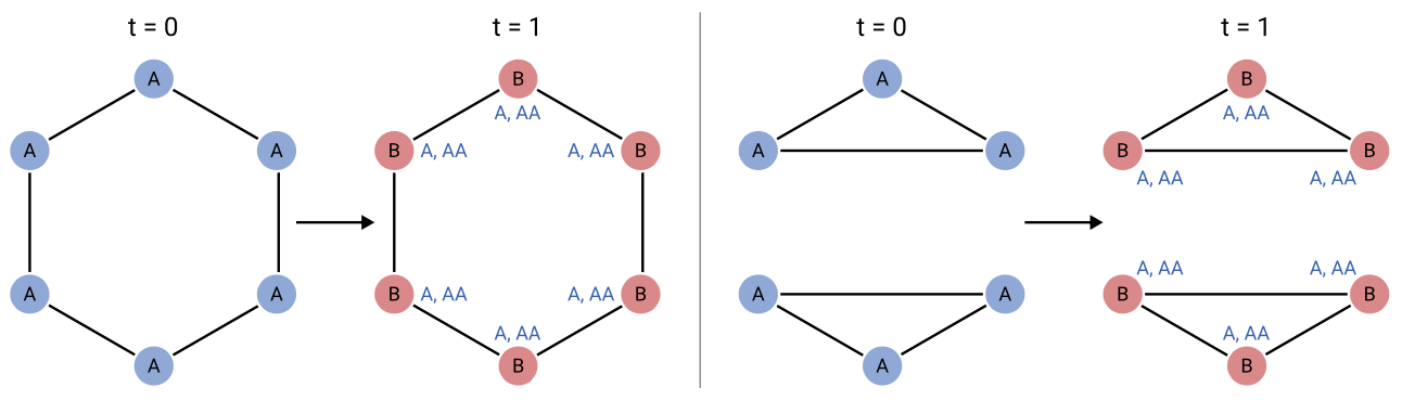
In addition, we extend our analysis to node-level viewpoints, and show that our model provably extends the WL subtree kernel (Eqn. 5) in differentiating different rooted local subgraphs.
Theorem 3.
Given a graph and . Denote as the set of exact matchings between subsets of neighborhoods of and (formally defined in (Shervashidze et al. 2011)). For such that , the following inequality holds.
| (20) | ||||
Moreover, there exists such that strict inequality holds.
Remarks. Both the WL subtree kernel and the Delta function return only 0 or 1, and therefore they are indicators of whether they deem local subgraphs rooted at and isomorphic. indicates , while , which indicates that is more powerful than .
Proof.
The first equality is shown by Theorem 1 in (Chen et al. 2020b). The second inequality is a direct corollary of Lemma 1.
To show that there exists such that strict inequality holds, we revisit the example in Fig. 2. Suppose consists of disjoint rings (i.e. 2-regular graphs), is in an , while is in an (), and node attributes are node degrees . Similar to Lemma 4, AWs with length would be sufficient such that . However, since node attributes and node degrees are all the same, the kernel mapping of the RWGK will follow . ∎
| Datasets | MUTAG | PROTEINS | PTC | IMDB-B | IMDB-M | COLLAB | BZR | COX2 | PROTEINS_full | Cora | Pubmed | PPI |
| Task | Graph | Graph | Graph | Graph | Graph | Graph | Graph | Graph | Graph | Node | Node | Node |
| Type | biochem | biochem | biochem | social | social | social | biochem | biochem | biochem | citation | citation | biochem |
| # Graphs | 188 | 1,113 | 344 | 1,000 | 1,500 | 5,000 | 405 | 467 | 1,113 | - | - | - |
| Avg # node | 18 | 39 | 26 | 20 | 13 | 74 | 36 | 41 | 39 | 2,708 | 19,717 | 14,755 |
| Avg # edge | 20 | 73 | 51 | 97 | 66 | 2,458 | 38 | 43 | 73 | 5,429 | 44,338 | 228,431 |
| # Class | 2 | 2 | 2 | 2 | 3 | 3 | 2 | 2 | 2 | 7 | 3 | 121 |
| Attribute Type | Disc. | Disc. | Disc. | No | No | No | Cont. | Cont. | Cont. | Disc. | Disc. | Disc. |
| Attr. Dim. | 1 | 1 | 1 | - | - | - | 3 | 3 | 29 | 1,433 | 500 | 50 |
6. Experiments
In this section, we introduce our empirical evaluations on GSKN. We first introduce experimental settings, before presenting various experimental results. Specifically, our evaluations consist of:
- •
Qualitative evaluation, where we carry out experiments on synthetic datasets to illustrate properties of GSKN in an intuitive manner.
- •
Quantitative evaluation, including graph classification and node classification on real-world graph datasets.
- •
Self evaluation, including analysis on model components, model parameters, and model efficiency.
6.1. Experimental Setup
We first introduce the datasets, comparison methods as well as settings for experimental evaluation.
Datasets We take the following benchmark datasets for evaluation.
- •
Graph Classification. We use the same benchmark datasets as in (Du et al. 2019), including 6 biochemical network datasets (MUTAG, PROTEINS, PTC, BZR, COX2, PROTEINS_full), and 3 social network datasets (IMDB-B, IMDB-M, and COLLAB). All biochemical network datasets have node attributes, with MUTAG, PROTEINS, PTC categorical and BZR, COX2, PROTEINS_full continuous, while none of the social network datasets have node features.
- •
Node Classification. We utilize citation networks (Cora, Pubmed (Kipf and Welling 2017)), and the protein interaction network (PPI).
Detailed dataset statistics and properties are listed in Table 1.
Baselines We take the following models as baselines for graph classification.
- •
LDP (Cai and Wang 2018) serves as a simple baseline based on degree information only.
- •
Graph Kernels, including the WL subtree kernel (Shervashidze et al. 2011), the Shortest Path (SP) Kernel (Borgwardt and Kriegel 2005), the RW kernel, GNTK (Du et al. 2019), RetGK (Zhang et al. 2018), DDGK(Al-Rfou et al. 2019), hashing graph kernels (HGK-WL, HGK-SP) (Morris et al. 2016), Graph2Vec (Narayanan et al. 2017), and WWL (Togninalli et al. 2019).
- •
GNNs, including PatchySAN (Niepert et al. 2016), GraphSAGE (Hamilton et al. 2017), GCN (Kipf and Welling 2017), GIN (Xu et al. 2018).
- •
AW based methods. We choose AWE (Ivanov and Burnaev 2018) and GraphSTONE (Long et al. 2020). AWE is based on skip-gram optimization on AW while GraphSTONE is an AW based GNN.
- •
Graph Kernel Networks, i.e. GCKN. We choose GCKN-Path, the strongest variant mentioned in (Chen et al. 2020b).
For node classification, we take GNNs as baselines, including GCN, GraphSAGE, GAT, GIN, GraLSP (Jin et al. 2020) and GraphSTONE. Among them, GraLSP and GraphSTONE also adopt AW to model substructure information.
Hyperparameter Settings We take 64-dimensional embeddings for all methods. The parameter settings of other baselines follow the recommended settings in relevant codes. For GSKN, we take in Eqn. 6 and 13, and choose anonymous walk length to be 5 or 6 depending on each dataset. Since the embeddings of GSKN come from the concatenation of kernel mappings of both AWGK and RWGK, we set the embedding size of each part as 32.
6.2. Synthetic Experiments for Proof-of-concept
| Model | Cycle | Wheel | Path | Ladder | Avg |
|---|---|---|---|---|---|
| RW Kernel | 62.6 | 100.0 | 74.3 | 100.0 | 84.8 |
| WL Kernel | 55.2 | 98.5 | 65.5 | 98.5 | 79.7 |
| SP Kernel | 61.9 | 100.0 | 43.8 | 92.2 | 75.5 |
| GIN | - | - | - | - | 90.0 |
| GCKN | 95.0 | 100.0 | 94.9 | 100.0 | 97.5 |
| GSKN | 99.5 | 100.0 | 99.5 | 100.0 | 99.7 |
| Model | Accuracy on Regular |
|---|---|
| GCKN | 50.0 |
| GSKN | 100.0 |
| Dataset | MUTAG | PROTEINS | PTC | IMDB-B | IMDB-M | COLLAB |
| LDP∗ | 88.9 9.6 | 73.3 5.7 | 63.8 6.6 | 68.5 4.0 | 42.9 3.7 | 76.1 1.4 |
| GCN∗ | 85.6 5.8 | 76.0 3.2 | 64.2 4.3 | 74.0 3.4 | 51.9 3.8 | 79.0 1.8 |
| PatchySAN∗ | 92.6 4.2 | 75.9 2.8 | 60.0 4.8 | 71.0 2.2 | 45.2 2.8 | 72.6 2.2 |
| GIN∗ | 89.4 5.6 | 76.2 2.8 | 64.6 7.0 | 75.1 5.1 | 52.3 2.8 | 80.2 1.9 |
| Graph2Vec | 83.1 6.5 | 73.9 2.6 | 59.6 5.9 | 51.1 4.0 | 47.4 3.1 | 52.6 1.9 |
| WL subtree∗ | 90.4 5.7 | 75.0 3.1 | 59.9 4.3 | 73.8 3.9 | 50.9 3.8 | 78.9 1.9 |
| RetGK∗ | 90.3 1.1 | 75.8 0.6 | 62.5 1.6 | 71.9 1.0 | 47.7 0.3 | 81.0 0.3 |
| GNTK∗ | 90.0 8.5 | 75.6 4.2 | 67.9 6.9 | 76.9 3.6 | 52.8 4.6 | 83.6 1.0 |
| DDGK | 85.0 1.1 | 72.3 4.7 | 65.7 6.3 | 63.2 4.5 | 49.1 2.9 | 75.4 1.8 |
| AWE | 88.9 6.4 | 71.5 4.9 | 63.8 8.5 | 73.1 4.1 | 53.1 3.9 | 73.6 2.3 |
| GraphSTONE | 67.2 8.9 | 59.1 4.4 | 55.6 5.9 | 57.2 2.7 | 35.9 3.2 | 55.7 2.4 |
| GCKN∗ | 92.8 6.1 | 76.0 3.4 | 67.3 5.0 | 75.9 3.7 | 53.0 3.1 | 82.3 1.1 |
| GSKN | 93.3 3.3 | 82.3 2.4 | 85.2 5.1 | 79.9 3.3 | 59.3 3.1 | 81.8 1.1 |
Model Cora Pubmed PPI Macro-f1 Micro-f1 Macro-f1 Micro-f1 Macro-f1 Micro-f1 30% 70% 30% 70% 30% 70% 30% 70% 30% 70% 30% 70% GCN∗ 79.84 81.09 80.97 81.94 76.93 77.21 76.42 77.49 12.57 12.62 40.40 40.44 GAT∗ 79.33 82.08 80.41 83.43 76.94 76.92 77.64 77.82 11.91 11.97 39.92 40.10 GraphSAGE∗ 80.52 81.90 82.13 83.17 76.61 77.24 77.36 77.84 11.81 12.41 39.80 40.08 GraLSP∗ 82.43 83.27 83.67 84.31 81.21 81.38 81.43 81.52 11.34 11.89 39.55 39.80 GraphSTONE∗ 82.78 83.54 83.88 84.73 78.61 78.87 79.53 81.03 15.55 15.91 43.60 43.64 GCKN 77.35 78.74 78.54 79.52 79.33 81.03 79.38 81.10 15.19 16.15 40.79 41.07 GSKN 77.44 79.32 78.87 80.55 80.06 81.98 80.26 82.13 19.19 20.06 43.71 43.82 Std (GSKN) / % 0.003 0.017 0.004 0.017 0.002 0.005 0.003 0.005 0.001 0.002 0.001 0.002
| Model | BZR | COX2 | PROTEINS_full |
| HGK-WL∗ | 78.6 0.6 | 78.1 0.5 | 75.9 0.2 |
| HGK-SP∗ | 76.4 0.7 | 72.6 1.2 | 75.8 0.2 |
| WWL∗ | 84.4 2.0 | 78.3 0.5 | 77.9 0.8 |
| GNTK∗ | 85.5 0.8 | 79.6 0.4 | 75.7 0.2 |
| GCKN∗ | 85.9 0.5 | 81.2 0.8 | 76.3 0.5 |
| GSKN | 85.3 0.4 | 82.3 0.6 | 81.9 0.3 |
To evaluate the expressiveness of GSKN against existing GKs and GNNs in a straightforward manner, we carry out experiments on two synthetic datasets with distinct structures as a simple proof-of-concept. As mentioned in Section 5, our model is theoretically stronger than the 1-WL test, and hence all MPGNNs.
In the first dataset Structure, we generate graphs with 4 different structures, including Cycle, Path, wheel, and Ladder. We show illustrations of these structures in Fig. 3. We generate graph instances for each class with their sizes . We also randomly add 10% edges in the generated graphs to incorporate some noise. We generate 100 graphs for each structure.
In the other synthetic dataset Regular, we generate 100 5-regular graphs with two types, one being connected 5-regular graphs with 20 nodes, Reg-20-5, and the other being two disjoint 5-regular graphs with 10 nodes each, 2-Reg-10-5. As stated in (Sato 2020), the 1-WL test, and hence MPGNNs cannot distinguish among different -regular graphs.
We compare our model with classical graph kernel methods on Structure, including the RW kernel, the WL kernel, and the SP kernel to show the general ability to distinguish among graph structures. We also compare against GNNs, including GIN and GCKN. For the WL kernel, we use degrees as node attributes following (Xu et al. 2018). Results are shown in Table 2. It can be shown that although all methods are almost 100% correct on Wheels and Ladders, the performances differ a lot on Cycle and Path. Among all the comparison methods, GSKN is able to outperform GCKN, the second strongest baseline by 5% on Cycle and Path, showing its better ability in distinguishing among different structures in general.
We further show that GSKN complements GNNs using Regular, a dataset where ordinary GNNs would be theoretically incapable. We show the results in Table 3. It can be shown that GCKN can do no better than guessing, while GSKN achieves 100% accuracy, showing the improvement of GSKN over GNNs.
6.3. Quantitative Evaluations
In this section, we present results on graph and node classification.
6.3.1. Graph Classification
We follow the same experimental protocols as (Du et al. 2019; Xu et al. 2018), and report the average accuracy and standard deviation over a 10-fold cross-validation on each dataset. We use the same data splits as (Xu et al. 2018) using their code. For classification, we use the SVM implementation of the Cyanure toolbox 44 4 http://julien.mairal.org/cyanure/.
We show the graph classification results in Table 4 and 6. Results marked with * are taken from (Du et al. 2019). We make the following findings.
- •
GSKN outperforms all baselines in all datasets except COLLAB. Specifically, GSKN achieves 6% improvement on PROTEINS and IMDB-M, and over 10% improvement on PTC. These improvements demonstrate the strength of GSKN in terms of graph classification.
- •
Compared with GCKN, our model is also able to achieve improvements on all datasets except COLLAB. Since GSKN extends GCKN, the improvements endorse the effectiveness of the AWGK, and its compatibility with GCKN.
- •
Compared with AWE and GraphSTONE, both of which use anonymous walks for graph representation, GSKN is also able to perform better. Specifically, AWE does not leverage node attributes, which limits its performance. GraphSTONE requires learning a topic model over AWs, which may require large graphs to ensure its effectiveness. By comparison, GSKN alleviates both drawbacks and achieves improvements with adequate modeling of anonymous walks, i.e. through the AWGK and its kernel mapping.
We also show the classification results on graphs with continuous node attributes in Table 6. On these datasets, GSKN also performs competitively (similar to GCKN and GNTK on BZR, 1% and 4% over the best baseline on COX2 and PROTEINS_full). We conclude that on a wide range of graph datasets can GSKN perform favorably against competitive baselines.
6.3.2. Node Classification
We then carry out node classification experiments. We follow the same experimental settings as (Long et al. 2020). Different fractions of nodes are sampled randomly for testing, leaving the rest for training. We use Logistic Regression as the classifier and take the macro and micro F1 scores for evaluation. The results are averaged over 10 independent runs.
The results are shown in Table 5. We make the following findings.
- •
GSKN achieves a 3-4% improvement on PPI over the best baseline (GraphSTONE), a similar performance as the best baseline (GraLSP) on Pubmed, and a 1% improvement over GCKN on Cora. Note that GCKN and GSKN do not use node-level supervision (e.g. node labels, edges), which may explain why both of them fail on Cora.
- •
Compared with GCKN, GSKN achieves a 1% improvement on Cora, a 1% improvement on Pubmed, and a 3-4% improvement on PPI. Since GCKN and GSKN are similarly trained, such improvements endorse the effectiveness of the kernel mapping of AWGK, and hence GSKN. As the node features are richer on Cora (1433 dims) and Pubmed (500 dims) than on PPI (50 dims), the additional structural information plays more significant roles on PPI than on Pubmed and Cora. Consequently, the improvements of GSKN are more evident on PPI than on Cora and Pubmed.
6.4. Model Analysis
We carry out model analysis, including ablation studies, efficiency, and parameter analysis to provide better understandings of GSKN. We use graph classification to reflect the performances of the model.
6.4.1. Ablation Studies
Corresponding to the theoretical analysis in Section 5, we carry out ablation studies to illustrate the strength of the AWGK kernel mapping by modifying input features and switching model components. We use different variants of our model, and run experiments on MUTAG, PROTEINS, and PTC.
We use four variants of our model.
- •
RW (degree) denotes the part with node degrees as input attributes. For graph classification, using node degrees as input attributes is a common practice, such as (Xu et al. 2018).
- •
AW denotes the part only.
- •
RW (attributes) denotes the part with node attributes as inputs.
- •
RW (attributes) + AW denotes , which is our full model formulation.
The results are shown in Table 7. It can be shown that alone is a competitive graph classifier, outperforming RW (attribute). Moreover, by adding AW to RW (attribute), performances are improved by 2% on MUTAG, 8% on PROTEINS, and 20% on PTC, showing the strength and compatibility of to .
6.4.2. Efficiency
We compare the efficiency of GSKN with several GK baselines: the RW Kernel, the WL Kernel, DDGK, and AWE. We also compare the efficiency of GSKN against GCKN. We train all models and report the time needed for convergence on a single machine equipped with a GPU with 12GB RAM.
Results are presented in Fig.8. It can be shown that GSKN is comparable with the most efficient graph kernels, e.g. the WL Kernel and Graph2Vec, and takes less than three times the time of GCKN. The results demonstrate that our model is highly efficient and thus scalable. By contrast, although AWE takes similar approaches (i.e. anonymous walks) as GSKN, GSKN is over 200 times more efficient than AWE, while being more accurate as shown in Table 4.
| Model | MUTAG | PROTEINS | PTC |
|---|---|---|---|
| RW (degree) | 86.7 | 71.8 | 58.5 |
| AW | 93.3 | 76.5 | 81.7 |
| RW (attribute) | 91.1 | 74.5 | 61.5 |
| RW (attribute) + AW | 93.3 | 82.3 | 85.2 |
| Model | MUTAG | IMDB-B | COLLAB |
| RW Kernel | 0.9 | 55.8 | > 48h |
| WL Kernel | 0.3 | 1.2 | 4.7 |
| Graph2Vec | 0.5 | 1.5 | 5.4 |
| DDGK | 70.2 | 360.1 | 2400.7 |
| AWE | 348.6 | 1824.5 | > 48h |
| GCKN | 1.1 | 1.3 | 6.5 |
| GSKN | 1.1 | 1.9 | 15.3 |


6.4.3. Parameter Analysis
We analyze four parameters in our model, anonymous walk length , the number of anonymous walks sampled per node , the bandwidth parameter of the Gaussian kernel in Eqn. 6, and the embedding size. We conduct experiments on PTC and PROTEINS, whose results are shown in Fig. 4 and 5 respectively. We make the following findings:
- •
Both parameters related to the , i.e. and need to be chosen appropriately instead of choosing arbitrarily large values. Specifically, and would be most appropriate, while excessively large values may compromise the performance by as much as 10%.
- •
Larger s in the Gaussian kernel (Eqn. 6) lead to better performance. Similar results are found in (Chen et al. 2020b), where they attribute the results to the fact that larger leads to a closer resemblance between the Gaussian kernel and the Dirac kernel.
- •
Larger embedding size does not necessarily lead to better performance. For GSKN, a size of 64 is appropriate.
7. Conclusion
In this paper, we propose GSKN, a GNN model with theoretically stronger ability than MPGNNs to distinguish graph structures. Specifically, we design our model based on anonymous walks (AWs), flexible substructure units, and derive it upon graph kernels (GKs), with efficient Nyström methods for computation. We theoretically demonstrate the stronger ability of GSKN to distinguish graph structures from both graph-level and node-level viewpoints. Correspondingly, both graph and node classification experiments are leveraged to evaluate our model, where our model outperforms a wide range of baselines, endorsing the analysis.
Acknowledgements.
This work was supported by the National Natural Science Foundation of China (Grant No. 61876006 and No. 61572041).References
- (1)
- Al-Rfou et al. (2019) Rami Al-Rfou, Bryan Perozzi, and Dustin Zelle. 2019. Ddgk: Learning graph representations for deep divergence graph kernels. In The World Wide Web Conference. 37–48.
- Arvind et al. (2020) Vikraman Arvind, Frank Fuhlbrück, Johannes Köbler, and Oleg Verbitsky. 2020. On Weisfeiler-Leman invariance: subgraph counts and related graph properties. J. Comput. System Sci. (2020).
- Bayati and Montanari (2011) Mohsen Bayati and Andrea Montanari. 2011. The dynamics of message passing on dense graphs, with applications to compressed sensing. IEEE Transactions on Information Theory 57, 2 (2011), 764–785.
- Borgwardt and Kriegel (2005) Karsten M Borgwardt and Hans-Peter Kriegel. 2005. Shortest-path kernels on graphs. In Fifth IEEE international conference on data mining (ICDM). IEEE, 8–pp.
- Bouritsas et al. (2020) Giorgos Bouritsas, Fabrizio Frasca, Stefanos Zafeiriou, and Michael M Bronstein. 2020. Improving Graph Neural Network Expressivity via Subgraph Isomorphism Counting. arXiv preprint arXiv:2006.09252 (2020).
- Cai and Wang (2018) Chen Cai and Yusu Wang. 2018. A simple yet effective baseline for non-attributed graph classification. arXiv preprint arXiv:1811.03508 (2018).
- Chen et al. (2019) Dexiong Chen, Laurent Jacob, and Julien Mairal. 2019. Biological sequence modeling with convolutional kernel networks. Bioinformatics 35, 18 (2019), 3294–3302.
- Chen et al. (2020b) Dexiong Chen, Laurent Jacob, and Julien Mairal. 2020b. Convolutional Kernel Networks for Graph-Structured Data. arXiv preprint arXiv:2003.05189 (2020).
- Chen et al. (2020a) Zhengdao Chen, Lei Chen, Soledad Villar, and Joan Bruna. 2020a. Can graph neural networks count substructures? arXiv preprint arXiv:2002.04025 (2020).
- Chung and Graham (1997) Fan RK Chung and Fan Chung Graham. 1997. Spectral graph theory. Number 92. American Mathematical Soc.
- Damke et al. (2020) Clemens Damke, Vitalik Melnikov, and Eyke Hüllermeier. 2020. A Novel Higher-order Weisfeiler-Lehman Graph Convolution. In Asian Conference on Machine Learning. PMLR, 49–64.
- Defferrard et al. (2016) Michaël Defferrard, Xavier Bresson, and Pierre Vandergheynst. 2016. Convolutional neural networks on graphs with fast localized spectral filtering. In Advances in neural information processing systems. 3844–3852.
- Du et al. (2019) Simon S Du, Kangcheng Hou, Russ R Salakhutdinov, Barnabas Poczos, Ruosong Wang, and Keyulu Xu. 2019. Graph neural tangent kernel: Fusing graph neural networks with graph kernels. In Advances in Neural Information Processing Systems. 5723–5733.
- Duvenaud et al. (2015) David K Duvenaud, Dougal Maclaurin, Jorge Iparraguirre, Rafael Bombarell, Timothy Hirzel, Alán Aspuru-Guzik, and Ryan P Adams. 2015. Convolutional networks on graphs for learning molecular fingerprints. In Advances in neural information processing systems. 2224–2232.
- Gärtner et al. (2003) Thomas Gärtner, Peter Flach, and Stefan Wrobel. 2003. On graph kernels: Hardness results and efficient alternatives. In Learning theory and kernel machines. Springer, 129–143.
- Gilmer et al. (2017) Justin Gilmer, Samuel S Schoenholz, Patrick F Riley, Oriol Vinyals, and George E Dahl. 2017. Neural message passing for Quantum chemistry. In Proceedings of the 34th International Conference on Machine Learning-Volume 70. 1263–1272.
- Granovetter (1973) Mark S Granovetter. 1973. The strength of weak ties. American journal of sociology 78, 6 (1973), 1360–1380.
- Hamilton et al. (2017) Will Hamilton, Zhitao Ying, and Jure Leskovec. 2017. Inductive representation learning on large graphs. In Advances in neural information processing systems. 1024–1034.
- Ivanov and Burnaev (2018) Sergey Ivanov and Evgeny Burnaev. 2018. Anonymous Walk Embeddings. In International Conference on Machine Learning. 2186–2195.
- Jin et al. (2020) Yilun Jin, Guojie Song, and Chuan Shi. 2020. GraLSP: Graph Neural Networks with Local Structural Patterns. In The Thirty-Fourth AAAI Conference on Artificial Intelligence, AAAI 2020, New York, NY, USA. AAAI Press, 4361–4368.
- Juszczyszyn et al. (2008) Krzysztof Juszczyszyn, Przemysław Kazienko, and Katarzyna Musiał. 2008. Local topology of social network based on motif analysis. In International Conference on Knowledge-Based and Intelligent Information and Engineering Systems. Springer, 97–105.
- Kang et al. (2012) U Kang, Hanghang Tong, and Jimeng Sun. 2012. Fast random walk graph kernel. In Proceedings of the SIAM international conference on data mining. SIAM, 828–838.
- Kipf and Welling (2017) Thomas Kipf and Max Welling. 2017. Semi-Supervised Classification with Graph Convolutional Networks. In International Conference of Learning Representations.
- Kriege et al. (2018) Nils M Kriege, Christopher Morris, Anja Rey, and Christian Sohler. 2018. A Property Testing Framework for the Theoretical Expressivity of Graph Kernels.. In IJCAI. 2348–2354.
- Lee et al. (2019) John Boaz Lee, Ryan Rossi, Xiangnan Kong, Sungchul Kim, Eunyee Koh, and Anup Rao. 2019. Graph convolutional networks with motif-based attention. In ACM International Conference on Information and Knowledge Management (CIKM).
- Lei et al. (2017) Tao Lei, Wengong Jin, Regina Barzilay, and Tommi Jaakkola. 2017. Deriving Neural Architectures from Sequence and Graph Kernels. In International Conference on Machine Learning. 2024–2033.
- Li et al. (2017) Pan Li, Hoang Dau, Gregory Puleo, and Olgica Milenkovic. 2017. Motif clustering and overlapping clustering for social network analysis. In IEEE INFOCOM 2017-IEEE Conference on Computer Communications. IEEE, 1–9.
- Liu et al. (2017) Zhichang Liu, Siva Krishna Mohan Nalluri, and J Fraser Stoddart. 2017. Surveying macrocyclic chemistry: from flexible crown ethers to rigid cyclophanes. Chemical Society Reviews 46, 9 (2017), 2459–2478.
- Long et al. (2020) Qingqing Long, Yilun Jin, Guojie Song, Yi Li, and Wei Lin. 2020. Graph Structural-topic Neural Network. In Proceedings of the 26th ACM SIGKDD International Conference on Knowledge Discovery & Data Mining. 1065–1073.
- Long et al. (2019) Qingqing Long, Yiming Wang, Lun Du, Guojie Song, Yilun Jin, and Wei Lin. 2019. Hierarchical Community Structure Preserving Network Embedding: A Subspace Approach. In Proceedings of the 28th ACM International Conference on Information and Knowledge Management. 409–418.
- Micali and Zhu (2016) Silvio Micali and Zeyuan Allen Zhu. 2016. Reconstructing markov processes from independent and anonymous experiments. Discrete Applied Mathematics 200 (2016), 108–122.
- Milo et al. (2002) Ron Milo, Shai Shen-Orr, Shalev Itzkovitz, Nadav Kashtan, Dmitri Chklovskii, and Uri Alon. 2002. Network motifs: simple building blocks of complex networks. Science 298, 5594 (2002), 824–827.
- Morris et al. (2016) Christopher Morris, Nils M Kriege, Kristian Kersting, and Petra Mutzel. 2016. Faster kernels for graphs with continuous attributes via hashing. In 2016 IEEE 16th International Conference on Data Mining (ICDM). IEEE, 1095–1100.
- Morris et al. (2019) Christopher Morris, Martin Ritzert, Matthias Fey, William L Hamilton, Jan Eric Lenssen, Gaurav Rattan, and Martin Grohe. 2019. Weisfeiler and leman go neural: Higher-order graph neural networks. In Proceedings of the AAAI Conference on Artificial Intelligence, Vol. 33. 4602–4609.
- Narayanan et al. (2017) Annamalai Narayanan, Mahinthan Chandramohan, Rajasekar Venkatesan, Lihui Chen, Yang Liu, and Shantanu Jaiswal. 2017. graph2vec: Learning distributed representations of graphs. arXiv preprint arXiv:1707.05005 (2017).
- Niepert et al. (2016) Mathias Niepert, Mohamed Ahmed, and Konstantin Kutzkov. 2016. Learning convolutional neural networks for graphs. In International conference on machine learning. 2014–2023.
- Paranjape et al. (2017) Ashwin Paranjape, Austin R Benson, and Jure Leskovec. 2017. Motifs in temporal networks. In Proceedings of the Tenth ACM International Conference on Web Search and Data Mining. 601–610.
- Pržulj (2007) Nataša Pržulj. 2007. Biological network comparison using graphlet degree distribution. Bioinformatics 23, 2 (2007), e177–e183.
- Sato (2020) Ryoma Sato. 2020. A survey on the expressive power of graph neural networks. arXiv preprint arXiv:2003.04078 (2020).
- Scarselli et al. (2008) Franco Scarselli, Marco Gori, Ah Chung Tsoi, Markus Hagenbuchner, and Gabriele Monfardini. 2008. The graph neural network model. IEEE Transactions on Neural Networks 20, 1 (2008), 61–80.
- Shawe-Taylor et al. (2004) John Shawe-Taylor, Nello Cristianini, et al. 2004. Kernel methods for pattern analysis. Cambridge university press.
- Shervashidze et al. (2011) Nino Shervashidze, Pascal Schweitzer, Erik Jan Van Leeuwen, Kurt Mehlhorn, and Karsten M Borgwardt. 2011. Weisfeiler-lehman graph kernels. Journal of Machine Learning Research 12, 9 (2011).
- Shervashidze et al. (2009) Nino Shervashidze, SVN Vishwanathan, Tobias Petri, Kurt Mehlhorn, and Karsten Borgwardt. 2009. Efficient graphlet kernels for large graph comparison. In Artificial Intelligence and Statistics. 488–495.
- Togninalli et al. (2019) Matteo Togninalli, Elisabetta Ghisu, Felipe Llinares-López, Bastian Rieck, and Karsten Borgwardt. 2019. Wasserstein weisfeiler-lehman graph kernels. In Advances in Neural Information Processing Systems. 6439–6449.
- Veličković et al. (2017) Petar Veličković, Guillem Cucurull, Arantxa Casanova, Adriana Romero, Pietro Lio, and Yoshua Bengio. 2017. Graph attention networks. arXiv preprint:1710.10903 (2017).
- Williams and Seeger (2001) Christopher KI Williams and Matthias Seeger. 2001. Using the Nyström method to speed up kernel machines. In Advances in neural information processing systems. 682–688.
- Wu et al. (2019) Felix Wu, Amauri Souza, Tianyi Zhang, Christopher Fifty, Tao Yu, and Kilian Weinberger. 2019. Simplifying Graph Convolutional Networks. In International Conference on Machine Learning. 6861–6871.
- Wu et al. (2020) Zonghan Wu, Shirui Pan, Fengwen Chen, Guodong Long, Chengqi Zhang, and S Yu Philip. 2020. A comprehensive survey on graph neural networks. IEEE Transactions on Neural Networks and Learning Systems (2020).
- Xu et al. (2018) Keyulu Xu, Weihua Hu, Jure Leskovec, and Stefanie Jegelka. 2018. How powerful are graph neural networks? arXiv preprint arXiv:1810.00826 (2018).
- Zhang et al. (2008) Kai Zhang, Ivor W Tsang, and James T Kwok. 2008. Improved Nyström low-rank approximation and error analysis. In Proceedings of the 25th international conference on Machine learning. 1232–1239.
- Zhang et al. (2013) Luming Zhang, Mingli Song, Zicheng Liu, Xiao Liu, Jiajun Bu, and Chun Chen. 2013. Probabilistic graphlet cut: Exploiting spatial structure cue for weakly supervised image segmentation. In Proceedings of the IEEE conference on computer vision and pattern recognition. 1908–1915.
- Zhang et al. (2018) Zhen Zhang, Mianzhi Wang, Yijian Xiang, Yan Huang, and Arye Nehorai. 2018. Retgk: Graph kernels based on return probabilities of random walks. In Advances in Neural Information Processing Systems. 3964–3974.