跳到论文正文
W Papers独立论文阅读器 arXiv:2104.02960 论文正文 计算阅读时间 · 0%
引用这篇论文根据当前论文元数据生成,正式投稿前建议核对。


License: arXiv.org perpetual non-exclusive license
arXiv:2104.02960v3 [math.ST] 12 Jan 2023

Community Detection with Contextual Multilayer Networks

Zongming Ma   and  Sagnik Nandy Note: Email: zongming@wharton.upenn.edu. Note: Email: sagnik@wharton.upenn.edu. Affiliation: University of Pennsylvania
Abstract

In this paper, we study community detection when we observe mm sparse networks and a high dimensional covariate matrix, all encoding the same community structure among nn subjects. In the asymptotic regime where the number of features pp and the number of subjects nn grow proportionally, we derive an exact formula of asymptotic minimum mean square error (MMSE) for estimating the common community structure in the balanced two block case using an orchestrated approximate message passing algorithm. The formula implies the necessity of integrating information from multiple data sources. Consequently, it induces a sharp threshold of phase transition between the regime where detection (i.e., weak recovery) is possible and the regime where no procedure performs better than random guess. The asymptotic MMSE depends on the covariate signal-to-noise ratio in a more subtle way than the phase transition threshold. In the special case of m=1m=1, our asymptotic MMSE formula complements the pioneering work [17] which found the sharp threshold when m=1m=1. A practical variant of the theoretically justified algorithm with spectral initialization leads to an estimator whose empirical MSEs closely approximate theoretical predictions over simulated examples.  
Keywords: clustering; contextual SBM; integrative data analysis; multilayer network; phase transition; stochastic block model; approximate message passing.

1 Introduction

Network data is a prevalent form of relational data. It appears in many different fields such as social science, economics, epidemiology, biological science, among others. Many networks come with inherent community structures. Nodes within the same community connect in different ways than nodes between different communities. The community labels of the nodes are usually unknown. It is of interest to uncover such latent community structures based on observed networks. This inference problem is usually called community detection which in essence is clustering of network nodes. The stochastic block model (SBM) [21] is a popular model for studying community detection. There has been a large literature on theoretical approaches, algorithmic, and application aspects of SBM’s. We refer interested readers to several recent survey papers [1, 18, 25] for more detailed accounts of this large and growing literature.

A more traditional clustering problem in statistics is clustering based on covariates, which is also a leading example of unsupervised learning. Standard techniques include, but are not limited to kk-means clustering, hierarchical clustering, and the EM algorithm. The multivariate Gaussian mixture model has been a popular model for theoretical study on this front which has received renewed interest in recent years. The model is closely related to the spiked covariance model [24] which is widely adopted in Random Matrix Theory.

Ever-growing techniques for data acquisition have led us to a new paradigm where one could have multiple data sets as multiple sources of information about the community structure. For instance, for a set of nn people, one could potentially have several social networks observed on them (Facebook, LinkedIn, etc.) together with a large collection of socioeconomic (and/or genomic, neuroimaging, etc.) covariates for each individual. This poses a new challenge: How can we best integrate information from these multiple sources to uncover the common underlying community structure?

When the network is at least part of the observation, there are two different scenarios. The first is where one observes multiple networks without any covariate. A practical example of this scenario was described in [14] where the nodes represent proteins, the edges in one network represent physical interactions between nodes and those in another network represent co-memberships in protein complexes. This scenario has been studied in the multilayer network literature. The arguably more interesting scenario is where one observes one or more networks together with a collection of covariates. In the pioneering work by Deshpande, et al. [17], the authors considered the case where the available data is an n×nn\times n adjacency matrix of an SBM and a high dimensional p×np\times n Gaussian covariate matrix, both containing the same balanced two block community structure. Under this stylized yet informative model, they rigorously established a sharp information-theoretic threshold for detecting the community structure (i.e., to uncover the community structure better than random guessing) when pp and nn tend to infinity proportionally and the average degree of the network diverges with nn. In addition, they proposed a heuristic algorithm which supports the information-theoretic threshold empirically. Subsequently, the sharp threshold was extended to the case where the average degree is bounded [27]. See also [11, 2] for investigations of spectral clustering and [38] for an SDP approach in similar models.

The present paper is motivated by two important questions that remain unanswered by [17].

  • •

    Multiple networks with or without covariates. How does the phase transition phenomenon found in [17] exhibit itself when one observes multiple networks with or without high-dimensional covariates? How does the threshold depend on individual signal-to-noise ratios in these multiple data sources?

  • •

    Precise characterization of the information-theoretic limit achieved by Bayes optimal
    estimator
    . Even in the special case considered by [17] where only one network is observed together with covariates, it is not clear what the information-theoretic limit of the performance by the best estimator is when the signal-to-noise ratio is above the phase transition threshold. The authors provided a spectral estimator that achieves nontrivial performance above the threshold. However, it is not Bayes optimal, and the exact form of the information-theoretic limit is unknown.

In this paper, we provide affirmative answers to both of the above questions. Without loss of generality, we propose to consider an observation model where one observes mm independent adjacency matrices from mm SBM’s and a high-dimensional Gaussian data-set with pp covariates, all carrying the same latent community structure (balanced two block). Focusing on this model and assuming that the average degrees diverge, our contributions are the following.

  • •

    Sharp phase transition threshold. We establish sharp thresholds for phase transition between the regime where detecting the community structure is feasible and the regime where no procedure performs better than random guess.

  • •

    Exact formula for asymptotic minimum mean square error (MMSE). We give an exact formula for the asymptotic MMSE achieved by the Bayes optimal estimator of the community structure.

To facilitate the derivation of asymptotic MMSE, we also provide convergence analysis of an orchestrated approximate message passing (AMP) algorithm with multiple parallel and information-sharing orbits. This could be of independent interest.

Last but not least, our results continue to hold for the special case where one only observes mm networks and there is no covariate. In this case, our model is reduced to a multilayer SBM. Results in [23, 33] provide sharp information-theoretic thresholds between the regimes of exact recovery (where the best procedure uncovers the community structure perfectly) and almost exact recovery (where the best procedure only makes mistakes on a vanishing proportion of nodes). In addition, [33, 37] derived the minimax rates of convergence that are sharp in exponents in the regime of almost exact recovery under the Hamming loss. In contrast, the present paper provides sharp thresholds for detection (a.k.a. weak recovery) and the exact asymptotic minimax risk under the squared error loss.

On the technical front, the main novelty of the present manuscript lies in designing an orchestrated AMP algorithm with multiple orbits that synchronizes the extraction of information about community structure from multiple data sources. In addition, we provide a rigorous proof of the almost sure convergence of the AMP average sequence. The idea underpinning the algorithm design is potentially applicable to other settings where the integration of information from multiple sources is needed.

The setting of the present paper can be reformulated as a multi-view spiked matrix model which has been studied in [7, 34]. The results of the aforementioned papers give the asymptotic MMSE of joint estimation of the covariates. More specifically, these papers have used the adaptive interpolation technique described in [6] to obtain the limit of per-vertex mutual information between data and both the community labels and the covariate means. Then they have used the I-MMSE identity to get the asymptotic MMSE for the joint estimation of the community labels and the covariate means. A different proof technique related to a similar model was described in [13], where the authors identified the limiting free energy as the viscosity solution to a certain Hamilton-Jacobi equation. In contrast to the foregoing papers, the present manuscript focuses on the optimal estimation of the community label vector only. The asymptotic joint estimation MMSE results in the foregoing papers do not lead to the asymptotic community label estimation MMSE we shall derive in this paper, since different priors (Rademacher vs. Gaussian) have been put on the community labels and the covariate means, respectively, while the connection between the joint and individual estimation MMSEs depend crucially on the choices of the priors. Due to the generality of the models considered, the asymptotic MMSE’s in [7, 34] were expressed in complicated variational forms with matrix arguments. In contrast, under the specific setting considered in the present manuscript, we shall obtain an explicit ‘single-letter’ characterization of the asymptotic MMSE. While it remains possible to derive asymptotic per-vertex mutual information between data and community labels alone by using the adaptive interpolation technique and further obtain the asymptotic MMSE result in the current paper by differentiation, our proof technique is constructive and hence is entirely different from the approaches in [7, 34, 13]. While those investigations found the limit of the free energy and used it to find the limit of the per-vertex mutual information, we shall use an AMP algorithm to explicitly construct a Bayes optimal sequence of estimators and directly obtain the asymptotic MMSE as the limiting mean squared error of that sequence. The limit of the per-vertex mutual information will be obtained as a side result of our calculations.

Paper organization

The rest of the paper is organized as follows. Section 2 introduces our observation models and presents key results on detection threshold and asymptotic MMSE along with introducing the new orchestrated AMP setup. It also lays out three major steps in the proof of main results, which are executed in Sections 3–5 in order, and formally summarized in Section 6. In Section 7 we collect the results on the asymptotics of the orchestrated AMP algorithm. In Section 8 we describe a practical algorithm for estimating the community labels using orchestrated AMP with appropriate spectral initialization and demonstrate its performance through simulations. Finally, we discuss the wider applicability of our techniques and discuss some potential future research directions in Section 9. The technical proofs are deferred to the appendices.

2 Detection Threshold and Asymptotic MMSE

2.1 Model

Suppose that nn subjects are partitioned into two disjoint groups (labeled by ±1\pm 1) according to an nn-dimensional vector 𝒙∗∈{±1}n\bm{x}^{*}\in\{\pm 1\}^{n}. Throughout the paper we assume that the elements xi∗x^{*}_{i}’s are i.i.d. Rademacher random variables which take values ±1\pm 1 with equal probability 12\frac{1}{2}.

The observed data consists of two parts. The first part is a collection of mm undirected networks on these nn subjects denoted by their adjacency matrices, 𝑮={𝑮(i):i∈[m]}\bm{G}=\{\bm{G}^{(i)}:i\in[m]\}. Throughout the paper, for any positive integer kk, we let [k]={1,…,k}[k]=\{1,\dots,k\}. The second part is a p×np\times n data matrix 𝑩\bm{B} where the ii-th column records the observed values of pp covariates on the ii-th subject. Conditional on an instance of 𝒙∗\bm{x}^{*}, the adjacency matrix 𝑮(i)\bm{G}^{(i)} has zero diagonal entries, and for all k≠lk\neq l, we assume

Gk​l(i)=Gl​k(i)∼i​n​d{Bern⁡(an(i)n),if xk∗=xl∗,Bern⁡(bn(i)n),if xk∗≠xl∗.{G}^{(i)}_{kl}={G}^{(i)}_{lk}\stackrel{{\scriptstyle ind}}{{\sim}}\begin{cases}\mathrm{Bern}\Big(\frac{\,a_{n}^{(i)}}{n}\Big),&\mbox{if $x^{*}_{k}=x^{*}_{l}$},\\ \mathrm{Bern}\Big(\frac{\,b_{n}^{(i)}}{n}\Big),&\mbox{if $x^{*}_{k}\neq x^{*}_{l}$}.\end{cases} (2.1)

For any ρ∈[0,1]\rho\in[0,1], Bern⁡(ρ)\mathrm{Bern}(\rho) denotes a Bernoulli distribution with success probability ρ\rho. Further, we assume that an(i)>bn(i)a_{n}^{(i)}>b_{n}^{(i)} for all n,i≥0n,i\geq 0. In addition, the data matrix 𝑩\bm{B} is assumed to admit the representation

𝑩=μn​𝒗∗​(𝒙∗)⊤+𝑹,\bm{B}=\sqrt{\frac{\mu}{n}}\,\bm{v^{*}}(\bm{x^{*}})^{\top}+\bm{R}, (2.2)

where 𝑹\bm{R} is an p×np\times n matrix consisting of i.i.d. standard Gaussian variates and 𝒗∗∼Np​(𝟎,𝑰p)\bm{v^{*}}\sim{N}_{p}(\bm{0},\bm{I}_{p}). Finally, we assume that conditional on 𝒙∗\bm{x}^{*}, 𝑮(1),…,𝑮(m)\bm{G}^{(1)},\dots,\bm{G}^{(m)} and 𝑩\bm{B} are mutually independent. In other words, conditional on 𝒙∗\bm{x}^{*}, the first part of our data consists of mm stochastic block models (a.k.a. a multi-layer stochastic block model with mm layers [20]) with a common community structure 𝒙∗\bm{x}^{*}. Given 𝒗∗\bm{v}^{*}, the columns of the covariate matrix 𝑩\bm{B} is also partitioned into two groups by 𝒙∗\bm{x}^{*}, where those corresponding to 𝒙i∗=+1\bm{x}^{*}_{i}=+1 are i.i.d. realizations of a Np​(μ/n​𝒗∗,𝑰p)N_{p}(\sqrt{{\mu}/{n}}\,\bm{v}^{*},\bm{I}_{p}) distribution, and those with 𝒙i∗=−1\bm{x}^{*}_{i}=-1 are i.i.d. random vectors following Np​(−μ/n​𝒗∗,𝑰p)N_{p}(-\sqrt{{\mu}/{n}}\,\bm{v}^{*},\bm{I}_{p}).

Our goal is to estimate 𝒙∗\bm{x}^{*} upon observing {𝑮(1),…,𝑮(m)}\{\bm{G}^{(1)},\dots,\bm{G}^{(m)}\} and 𝑩\bm{B}. We focus on an asymptotic regime where as n→∞n\to\infty, mm is fixed and

limn→∞pn=1c∈(0,∞).\lim_{n\to\infty}\frac{p}{n}=\frac{1}{c}\in(0,\infty). (2.3)

For each 1≤i≤m1\leq i\leq m, define

p¯n(i)=an(i)+bn(i)2​n,Δn(i)=an(i)−bn(i)2​n,λn(i)=n​(an(i)−bn(i))2(an(i)+bn(i))​(2​n−an(i)−bn(i)).\widebar{p}^{(i)}_{n}=\frac{a_{n}^{(i)}+b_{n}^{(i)}}{2n},\quad\Delta^{(i)}_{n}=\frac{a_{n}^{(i)}-b_{n}^{(i)}}{2n},\quad\lambda_{n}^{(i)}=\frac{n(a^{(i)}_{n}-b^{(i)}_{n})^{2}}{(a^{(i)}_{n}+b^{(i)}_{n})(2n-a^{(i)}_{n}-b^{(i)}_{n})}. (2.4)

We further assume that μ≥0\mu\geq 0 is a fixed constant while

limn→∞n​p¯n(i)​(1−p¯n(i))=∞,and\displaystyle\lim_{n\to\infty}n\widebar{p}^{(i)}_{n}(1-\widebar{p}^{(i)}_{n})=\infty,\quad\mbox{and} (2.5)
λn(i)=λ(i)∈(0,∞),for all n,i.\displaystyle\hskip 25.29494pt\lambda_{n}^{(i)}=\lambda^{(i)}\in(0,\infty),\quad\mbox{for all $n,i$.} (2.6)

For brevity, we let

𝝀=(λ(1),…,λ(m))andλ=∑i=1mλ(i)\bm{\lambda}=(\lambda^{(1)},\ldots,\lambda^{(m)})\quad\mbox{and}\quad\lambda=\sum_{i=1}^{m}\lambda^{(i)} (2.7)

in the rest of this paper. For convenience, we shall further assume that there are some constants r(1),…,r(m)∈(0,1)r^{(1)},\ldots,r^{(m)}\in(0,1) such that

∑i=1mr(i)=1andλ(i)=r(i)​λ,for all i.\sum_{i=1}^{m}r^{(i)}=1\quad\mbox{and}\quad\lambda^{(i)}=r^{(i)}\lambda,\quad\mbox{for all $i$.} (2.8)

2.2 Detection Threshold

For every fixed nn, λ\lambda and μ\mu, we define

Overlapn(𝝀,μ)=sups^n:𝒢n×ℬn→{±1}n1n𝔼|⟨𝒙∗,s^n(𝑮,𝑩)⟩|.\mathrm{Overlap}_{n}(\bm{\lambda},\mu)=\sup_{\widehat{s}_{n}:\mathcal{G}_{n}\times\mathcal{B}_{n}\rightarrow\{\pm 1\}^{n}}\frac{1}{n}\,\mathbb{E}\left|\left\langle\bm{x^{*}},\hat{s}_{n}(\bm{G},\bm{B})\right\rangle\right|. (2.9)

Here 𝒢n\mathcal{G}_{n} is the set of all collections of mm undirected networks on nn vertices, ℬn\mathcal{B}_{n} is the set of all p×np\times n real-valued matrices, and s^n​(𝑮,𝑩)\widehat{s}_{n}(\bm{G},\bm{B}) is a generic estimator of the community vector 𝒙∗\bm{x^{*}} based on observing 𝑮\bm{G} and 𝑩\bm{B}.

We say detection (a.k.a. weak recovery) of 𝒙∗\bm{x}^{*} is possible if

lim infn→∞Overlapn​(𝝀,μ)>0.\liminf_{n\rightarrow\infty}\mathrm{Overlap}_{n}(\bm{\lambda},\mu)>0. (2.10)

Otherwise, we perform no better than random guessing. Indeed, if we simply estimate by random guessing, then our estimator is essentially a vector 𝒙\bm{x} with i.i.d. Rademacher entries that is independent of 𝒙∗\bm{x}^{*}, and we have 1n​𝔼​|⟨𝒙∗,𝒙⟩|→0\frac{1}{n}\mathbb{E}|\langle\bm{x}^{*},\bm{x}\rangle|\to 0.

The following theorem characterizes the phase transition of detection under our model.

Theorem 2.1.

Let the data be generated by (2.1) and (2.2). Suppose that as n→∞n\to\infty, (2.3), (2.5), (2.6) and (2.8) hold. Then we have

lim supn→∞Overlapn​(𝝀,μ)=0,\displaystyle\limsup_{n\rightarrow\infty}\mathrm{Overlap}_{n}(\bm{\lambda},\mu)=0, if λ+μ2c≤1,\displaystyle\mbox{if $\lambda+\frac{\mu^{2}}{c}\leq 1$}, (2.11)
lim infn→∞Overlapn​(𝝀,μ)>0,\displaystyle\liminf_{n\rightarrow\infty}\mathrm{Overlap}_{n}(\bm{\lambda},\mu)>0, if λ+μ2c>1.\displaystyle\mbox{if $\lambda+\frac{\mu^{2}}{c}>1$}.

where λ\lambda is defined in (2.7).

Proof.

The theorem follows from our later Theorem 2.2 and (2.13). ∎

Remark 2.1.

Note that r(1),…,r(m)∈(0,1)r^{(1)},\ldots,r^{(m)}\in(0,1) are allowed to take any values as long as (2.8) holds.

The foregoing theorem determines a sharp detection threshold in terms of the joint signal-to-noise ratio (SNR) contained in the two different data sources, namely the mm networks and the data matrix. Here λ\lambda can be understood as the joint SNR of the mm networks. The phase transition described in (2.11) asserts that the joint SNR of the two parts has an additive form λ+μ2/c\lambda+\mu^{2}/c. In the special case of m=1m=1, Theorem 2.1 reconstructs the threshold found in [17]. When m=0m=0, it coincides with the famous Baik–Ben Arous–Peche phase transition for PCA [4, 5, 32]. When μ=0\mu=0, we could simply discard the data matrix 𝑩\bm{B} as it contains no information about 𝒙∗\bm{x}^{*} and Theorem 2.1 leads to a new detection threshold for multi-layer stochastic block models.

2.3 Asymptotic MMSE

We now seek a more precise characterization of the optimal estimator of 𝒙∗\bm{x}^{*} based on observing 𝑮\bm{G} and 𝑩\bm{B}, where the optimality is measured through the mean square error.

Minimum mean square error

To this end, define the (matrix) minimum mean square error for estimating the community labels from (𝑮,𝑩)(\bm{G},\bm{B}) as

𝖬𝖬𝖲𝖤n(𝝀,μ)=1n2𝔼[∥𝒙∗(𝒙∗)⊤−𝔼[𝒙∗(𝒙∗)⊤|𝑮,𝑩]∥F2].\mathsf{MMSE}_{n}(\bm{\lambda},\mu)=\frac{1}{\,n^{2}}\mathbb{E}\left[\|\bm{x^{*}}(\bm{x^{*}})^{\top}-\mathbb{E}\left[\bm{x^{*}}(\bm{x^{*}})^{\top}\middle|\,\bm{G},\bm{B}\right]\|^{2}_{F}\right]. (2.12)

Following the lines of the proof of Lemma 4.6 in [15], one has

1−𝖬𝖬𝖲𝖤n(𝝀,μ)+O(n−1)≤Overlapn(𝝀,μ)≤1−𝖬𝖬𝖲𝖤n​(𝝀,μ)+O(n−1/2).1-\mathsf{MMSE}_{n}(\bm{\lambda},\mu)+O(n^{-1})\leq\mathrm{Overlap}_{n}(\bm{\lambda},\mu)\leq\sqrt{1-\mathsf{MMSE}_{n}(\bm{\lambda},\mu)}+O(n^{-1/2}). (2.13)

In particular, Overlapn​(𝝀,μ)→0\mathrm{Overlap}_{n}(\bm{\lambda},\mu)\to 0 if and only if 𝖬𝖬𝖲𝖤n​(𝝀,μ)→1\mathsf{MMSE}_{n}(\bm{\lambda},\mu)\to 1. Therefore, a more precise characterization of the overlap than that in Theorem 2.1 can be made if we could describe the exact asymptotic behavior of 𝖬𝖬𝖲𝖤n​(𝝀,μ)\mathsf{MMSE}_{n}(\bm{\lambda},\mu).

A scalar Gaussian model

As a useful device for describing the asymptotic behavior of 𝖬𝖬𝖲𝖤n​(𝝀,μ)\mathsf{MMSE}_{n}(\bm{\lambda},\mu), we follow [29, 16, 15] to introduce the following scalar Gaussian model:

Y=Y⁡(η)=η​X0+Z0,Y=Y(\eta)=\sqrt{\eta}X_{0}+Z_{0}, (2.14)

where X0∼RademacherX_{0}\sim\mbox{Rademacher} and Z0∼N⁡(0,1)Z_{0}\sim N(0,1). In (2.14), every term is a scalar. We assume knowledge of η\eta and the goal is to estimate X0X_{0} based on the observed YY. For this model, we can compute the mutual information between X0X_{0} and YY and the minimum mean square error for estimating X0X_{0} respectively as

I⁡(η)\displaystyle\mathrm{I}(\eta) =𝔼⁡[d​pY|X0​(Y⁡(η)∣X0)d​pY​(Y⁡(η))]=η−𝔼⁡[log⁡cosh⁡(η+η​Z0)],\displaystyle=\mathbb{E}\left[\frac{dp_{Y\mid X_{0}}(Y(\eta)\mid X_{0})}{dp_{Y}(Y(\eta))}\right]=\eta-\mathbb{E}\left[\log\cosh(\eta+\sqrt{\eta}Z_{0})\right], (2.15)
mmse⁡(η)\displaystyle\mathrm{mmse}(\eta) =𝔼​[X0−𝔼⁡(X0∣Y⁡(η))]2=1−𝔼⁡[tanh2⁡(η+η​Z0)].\displaystyle=\mathbb{E}\left[X_{0}-\mathbb{E}(X_{0}\mid Y(\eta))\right]^{2}=1-\mathbb{E}\left[\tanh^{2}(\eta+\sqrt{\eta}Z_{0})\right]. (2.16)
Representation of the asymptotic MMSE

With the foregoing definitions in (2.14), (2.15) and (2.16), we define z∗=z∗​(λ,μ)z_{*}=z_{*}(\lambda,\mu) as the largest non-negative solution to

z=1−mmse⁡(λ​z+μ2c​z1+μ​z).z=1-\mathrm{mmse}\left(\lambda z+\frac{\mu^{2}}{c}\;\frac{z}{1+\mu z}\right). (2.17)

The following theorem gives a precise characterization of the limiting behavior of 𝖬𝖬𝖲𝖤n​(𝝀,μ)\mathsf{MMSE}_{n}(\bm{\lambda},\mu).

Theorem 2.2.

Suppose that the conditions in Theorem 2.1 hold. Then we have

limn→∞𝖬𝖬𝖲𝖤n​(𝝀,μ)=1−z∗2​(λ,μ),\lim\limits_{n\rightarrow\infty}\mathsf{MMSE}_{n}(\bm{\lambda},\mu)=1-z^{2}_{*}(\lambda,\mu), (2.18)

where λ\lambda is defined by (2.7). This implies

  1. 1.

    If λ+μ2/c≤1\lambda+\mu^{2}/c\leq 1,

    limn→∞𝖬𝖬𝖲𝖤n​(𝝀,μ)=1,\lim\limits_{n\rightarrow\infty}\mathsf{MMSE}_{n}(\bm{\lambda},\mu)=1, (2.19)
  2. 2.

    If λ+μ2/c>1\lambda+\mu^{2}/c>1,

    limn→∞𝖬𝖬𝖲𝖤n​(𝝀,μ)<1.\lim\limits_{n\rightarrow\infty}\mathsf{MMSE}_{n}(\bm{\lambda},\mu)<1. (2.20)
Refer to caption
Refer to caption
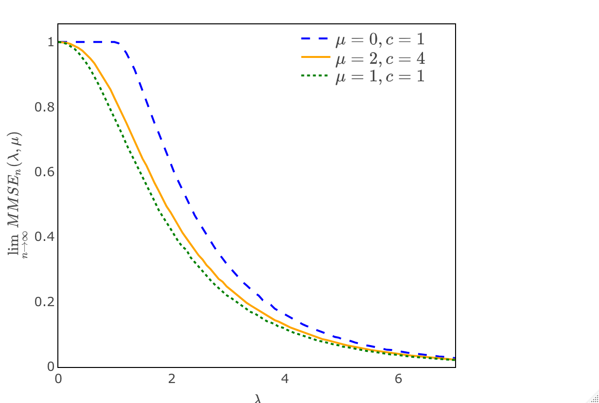
Figure 1: Plots of asymptotic MMSE. Left panel: Asymptotic MMSE as a function of λ\lambda for fixed μ\mu and cc combinations. Right panel: Asymptotic MMSE as a function of μ\mu for fixed λ\lambda and cc combinations.
Remark 2.2.

If λ+μ2/c>1\lambda+\mu^{2}/c>1, then z∗​(λ,μ)z_{*}(\lambda,\mu), the largest non-negative solution to (2.17) is strictly greater than zero. Consequently, the limit of MMSE is strictly less than 11, or equivalently, we strictly perform better than random guessing.

Remark 2.3.

Together with (2.13), phase transition of matrix MMSE for estimating 𝒙∗\bm{x}^{*} in Theorem 2.2 implies the phase transition of the overlap in Theorem 2.1.

Remark 2.4.

By Theorems 2.1 and 2.2, the parameter 𝝀\bm{\lambda} affects the asymptotic behavior of both Overlapn\mathrm{Overlap}_{n} and 𝖬𝖬𝖲𝖤n\mathsf{MMSE}_{n} only through λ\lambda. So from here on, we shall slightly abuse notation to also write Overlapn​(λ,μ)\mathrm{Overlap}_{n}(\lambda,\mu) and 𝖬𝖬𝖲𝖤n​(λ,μ)\mathsf{MMSE}_{n}(\lambda,\mu), which can be viewed as fixing a set of r(i)r^{(i)}’s in (2.8) and hence treating Overlapn\mathrm{Overlap}_{n} and 𝖬𝖬𝖲𝖤n\mathsf{MMSE}_{n} as functions of λ\lambda and μ\mu only for this fixed set of r(i)r^{(i)}’s.

In Figure 1, we show how limn→∞𝖬𝖬𝖲𝖤n​(λ,μ)\lim_{n\rightarrow\infty}\mathsf{MMSE}_{n}(\lambda,\mu) behaves as a function of λ\lambda for different values of μ\mu and cc, and as a function of μ\mu for different values of λ\lambda and cc. It is worth noting that even for the same values of λ\lambda and μ2/c\mu^{2}/c, asymptotic MMSE’s could differ, as its dependence on the three parameters is more subtle than the phase transition threshold.

2.4 Outline of Proof

We now outline the three major steps in the proof of Theorem 2.2. We follow the same overall proof structure as in [15]. Compared with [17] and [15], our major novelty lies in the proposal of an orchestrated AMP algorithm which synchronizes updates about community structure from multiple data sources.

Gaussian approximation

In the first step, we define a Gaussian observation model whose asymptotic per-vertex mutual information about 𝒙∗\bm{x}^{*} is the same as that in the original observation model in (2.1)–(2.2). To this end, let {𝒀(i):i∈[m]}\left\{\bm{Y}^{(i)}:i\in[m]\right\} be a collection of symmetric Gaussian matrices defined as

𝒀(i)=λ(i)n​𝒙∗​(𝒙∗)⊤+𝒁(i),i∈[m],\bm{Y}^{(i)}=\sqrt{\frac{\,\lambda^{(i)}}{n}}\,\bm{x^{*}}(\bm{x^{*}})^{\top}+\bm{Z}^{(i)},\quad i\in[m], (2.21)

where 𝒁(i)\bm{Z}^{(i)}’s are i.i.d. Gaussian Wigner matrices. In other words, each 𝒁(i)\bm{Z}^{(i)} is symmetric and

Zk​l(i)=Zl​k(i)∼{N⁡(0,1)if k≠l.N⁡(0,2)if k=l.Z^{(i)}_{kl}=Z^{(i)}_{lk}\sim\begin{cases}N\left(0,1\right)&\mbox{if $k\neq l$.}\\ N\left(0,2\right)&\mbox{if $k=l$.}\end{cases} (2.22)

We shall denote the collection of 𝒀(i)\bm{Y}^{(i)}’s by 𝒀\bm{Y}, i.e.

𝒀={𝒀(i):i∈[m]}.\bm{Y}=\{\bm{Y}^{(i)}:i\in[m]\}.

Using Lindeberg’s interpolation argument, we show that the per-vertex mutual information between 𝒙∗\bm{x}^{*} and the Gaussian observation model {𝒀,𝑩}\{\bm{Y},\bm{B}\} is asymptotically the same as that between 𝒙∗\bm{x}^{*} and the original observation {𝑮,𝑩}\{\bm{G},\bm{B}\}, in the sense that

1n​I​(𝒙∗,𝑮,𝑩)−1n​I​(𝒙∗,𝒀,𝑩)→0asn→∞.\frac{1}{n}I(\bm{x}^{*};\bm{G},\bm{B})-\frac{1}{n}I(\bm{x}^{*};\bm{Y},\bm{B})\to 0\quad\mbox{as}\quad n\to\infty. (2.23)

As a final reduction in our first step, we shall show that

I⁡(𝒙∗,𝑻,𝑩)=I⁡(𝒙∗,𝒀,𝑩)I(\bm{x}^{*};\bm{T},\bm{B})=I(\bm{x}^{*};\bm{Y},\bm{B}) (2.24)

where for λ\lambda defined in (2.7) and 𝒁\bm{Z}, a Gaussian Wigner matrix, as in (2.22)

𝑻=𝑻⁡(λ)=λn​𝒙∗​(𝒙∗)⊤+𝒁.\bm{T}=\bm{T}(\lambda)=\sqrt{\frac{\lambda}{n}}\,\bm{x^{*}}(\bm{x^{*}})^{\top}+\bm{Z}. (2.25)
Asymptotic I-MMSE relation

For Gaussian observation models, one has the famous I-MMSE relation [19]. For instance, for the Gaussian observation (𝑻,𝑩)(\bm{T},\bm{B}), define

𝖦𝖬𝖬𝖲𝖤n(λ,μ)=1n2𝔼‖𝒙∗(𝒙∗)⊤−𝔼[𝒙∗(𝒙∗)⊤|𝑻,𝑩]‖F2.\mathsf{GMMSE}_{n}(\lambda,\mu)=\frac{1}{\,n^{2}}\,\mathbb{E}\left\|\bm{x}^{*}(\bm{x}^{*})^{\top}-\mathbb{E}[\bm{x}^{*}(\bm{x}^{*})^{\top}\,|\,\bm{T},\bm{B}]\right\|_{F}^{2}. (2.26)

Then the I-MMSE relation refers to the identity

1n​dd​λ​I​(𝒙∗​(𝒙∗)⊤,𝑻,𝑩)=14​𝖦𝖬𝖬𝖲𝖤n​(λ,μ).\frac{1}{n}\frac{d}{d\lambda}I\left(\bm{x}^{*}(\bm{x}^{*})^{\top};\bm{T},\bm{B}\right)=\frac{1}{4}\mathsf{GMMSE}_{n}(\lambda,\mu). (2.27)

See Section C for a proof of (2.27). On the other hand, we shall derive the following asymptotic counterpart of (2.27) for the original observation model {𝑮,𝑩}\{\bm{G},\bm{B}\}:

1n​dd​λ​I​(𝒙∗,𝑮,𝑩)−14​𝖬𝖬𝖲𝖤n​(λ,μ)→0.\frac{1}{n}\frac{d}{d\lambda}I(\bm{x}^{*};\bm{G},\bm{B})-\frac{1}{4}\mathsf{MMSE}_{n}(\lambda,\mu)\to 0. (2.28)

Furthermore, (263) of [15] implies for 𝑲=𝒀\bm{K}=\bm{Y} and 𝑻\bm{T}

1n​I​(𝒙∗,𝑲,𝑩)−1n​I​(𝒙∗​(𝒙∗)⊤,𝑲,𝑩)→0.\frac{1}{n}I(\bm{x}^{*};\bm{K},\bm{B})-\frac{1}{n}I\left(\bm{x}^{*}(\bm{x}^{*})^{\top};\bm{K},\bm{B}\right)\to 0. (2.29)

Together with (2.23) and the fundamental theorem of calculus, (2.28) and (2.29) establish the asymptotic equivalence of the MMSE’s in the two models. Hence, the proof of Theorem 2.2 reduces to finding the exact asymptotic limit of 𝖦𝖬𝖬𝖲𝖤n​(λ,μ)\mathsf{GMMSE}_{n}(\lambda,\mu). To this end, we turn to Approximate Message Passing (AMP).

Approximate message passing and MMSE in the Gaussian observation model

To obtain the “large nn” limit of 𝖦𝖬𝖬𝖲𝖤n​(λ,μ)\mathsf{GMMSE}_{n}(\lambda,\mu), we design the following orchestrated AMP algorithm where we extract information about 𝒙∗\bm{x}^{*} from both the data sources.

Let 𝒖0=𝒙0=𝟎\bm{u}^{0}=\bm{x}^{0}=\bm{0}, 𝑻\bm{T} be as in (2.25) and 𝑩\bm{B} be as in (2.2). Fix any ε∈(0,1)\varepsilon\in(0,1). We define two companion AMP orbits {𝒗t,𝒖t+1}\{\bm{v}^{t},\bm{u}^{t+1}\} and {𝒙t+1}\{\bm{x}^{t+1}\}, for t=0,1,2,…,t=0,1,2,\ldots, characterized by the sensing matrices 𝑻\bm{T} and 𝑩\bm{B} respectively, as follows

𝒗t\displaystyle\bm{v}^{t} =𝑩p​ft​(𝒖t,𝒙t,𝒙0​(ε))−pt​gt−1​(𝒗t−1,𝒗0​(ε)),\displaystyle=\frac{\bm{B}}{\sqrt{p}}f_{t}(\bm{u}^{t},\bm{x}^{t},\bm{x}_{0}(\varepsilon))-p_{t}g_{t-1}(\bm{v}^{t-1},\bm{v}_{0}(\varepsilon)), (2.30)
𝒖t+1\displaystyle\bm{u}^{t+1} =𝑩⊤p​gt​(𝒗t,𝒗0​(ε))−ct​ft​(𝒖t,𝒙t,𝒙0​(ε)),\displaystyle=\frac{\,\bm{B}^{\top}}{\sqrt{p}}g_{t}(\bm{v}^{t},\bm{v}_{0}(\varepsilon))-c_{t}f_{t}(\bm{u}^{t},\bm{x}^{t},\bm{x}_{0}(\varepsilon)),

and

𝒙t+1=𝑻n​ft​(𝒖t,𝒙t,𝒙0​(ε))−dt​ft−1​(𝒖t−1,𝒙t−1,𝒙0​(ε)).\bm{x}^{t+1}=\frac{\bm{T}}{\sqrt{n}}f_{t}(\bm{u}^{t},\bm{x}^{t},\bm{x}_{0}(\varepsilon))-d_{t}f_{t-1}(\bm{u}^{t-1},\bm{x}^{t-1},\bm{x}_{0}(\varepsilon)). (2.31)

Here 𝒙0​(ε)=(x0,1​(ε),…,x0,n​(ε))⊤=(B1​x1∗,…,Bn​xn∗)⊤\bm{x}_{0}(\varepsilon)=(x_{0,1}(\varepsilon),\ldots,x_{0,n}(\varepsilon))^{\top}=(B_{1}x^{*}_{1},\ldots,B_{n}x^{*}_{n})^{\top} where BiB_{i}’s are i.i.d. Bern⁡(ε)\mathrm{Bern}(\varepsilon) and 𝒗0​(ε)=(v0,1​(ε),…,v0,p​(ε))⊤=(B~1​v1∗,…,B~p​vp∗)⊤\bm{v}_{0}(\varepsilon)=(v_{0,1}(\varepsilon),\ldots,v_{0,p}(\varepsilon))^{\top}=(\widetilde{B}_{1}v^{*}_{1},\ldots,\widetilde{B}_{p}v^{*}_{p})^{\top} where B~j\widetilde{B}_{j}’s are i.i.d. Bern⁡(ε)\mathrm{Bern}(\varepsilon). Next, we define

gt​(𝒗t,𝒗0)\displaystyle g_{t}(\bm{v}^{t},\bm{v}_{0}) =(gt​(v1t,v0,1​(ε)),…,gt​(vpt,v0,p​(ε)))⊤,\displaystyle=(g_{t}(v^{t}_{1},v_{0,1}(\varepsilon)),\ldots,g_{t}(v^{t}_{p},v_{0,p}(\varepsilon)))^{\top}, (2.32)
ft​(𝒖t,𝒙t,𝒙0)\displaystyle f_{t}(\bm{u}^{t},\bm{x}^{t},\bm{x}_{0}) =(ft​(u1t,x1t,x0,1​(ε)),…,ft​(unt,xnt,x0,n​(ε)))⊤,\displaystyle=(f_{t}(u^{t}_{1},x^{t}_{1},x_{0,1}(\varepsilon)),\ldots,f_{t}(u^{t}_{n},x^{t}_{n},x_{0,n}(\varepsilon)))^{\top},

and

ct=1p​∑i=1p∂gt∂v​(vit,v0,i​(ε)),pt=cn​∑i=1n∂ft∂u​(uit,xit,x0,i​(ε)),dt=1n​∑i=1n∂ft∂x​(uit,xit,x0,i​(ε)),c_{t}=\frac{1}{p}\sum\limits_{i=1}^{p}\frac{\partial g_{t}}{\partial v}(v^{t}_{i},v_{0,i}(\varepsilon)),\quad p_{t}=\frac{c}{n}\sum\limits_{i=1}^{n}\frac{\partial f_{t}}{\partial u}(u^{t}_{i},x^{t}_{i},x_{0,i}(\varepsilon)),\quad d_{t}=\frac{1}{n}\sum\limits_{i=1}^{n}\frac{\partial f_{t}}{\partial x}(u^{t}_{i},x^{t}_{i},x_{0,i}(\varepsilon)), (2.33)

where g−1g_{-1} is the zero function, and ft:ℝ3→ℝf_{t}:\mathbb{R}^{3}\rightarrow\mathbb{R} and gt:ℝ2→ℝg_{t}:\mathbb{R}^{2}\rightarrow\mathbb{R} for t∈ℕ∪{0}t\in\mathbb{N}\cup\{0\} are defined as follows:

ft​(x,y,z)\displaystyle f_{t}(x,y,z) =𝔼[X0|αt−1X0+τt−1Z1=x,μtX0+σtZ2=y,X0(ε)=z],\displaystyle=\mathbb{E}\left[X_{0}|\alpha_{t-1}X_{0}+\tau_{t-1}Z_{1}=x,\mu_{t}X_{0}+\sigma_{t}Z_{2}=y,X_{0}(\varepsilon)=z\right], (2.34)
gt​(x,z)\displaystyle g_{t}(x,z) =𝔼[V0|βtV0+ϑtZ3=x,V0(ε)=z].\displaystyle=\mathbb{E}\left[V_{0}|\beta_{t}V_{0}+\vartheta_{t}Z_{3}=x,V_{0}(\varepsilon)=z\right]. (2.35)

In the above definitions (2.34) and (2.35)

X0∼Rademacher, X0​(ε)=B⁡(ε)​X0 with B⁡(ε)∼Bern⁡(ε),\displaystyle\mbox{$X_{0}\sim\mbox{Rademacher}$, $X_{0}(\varepsilon)=B(\varepsilon)X_{0}$ with $B(\varepsilon)\sim\mathrm{Bern}(\varepsilon)$}, (2.36)
V0​(ε)=B~​(ε)​V0 with B~​(ε)∼Bern​(ε), V0,Z1,Z2,Z3∼N⁡(0,1), and\displaystyle\mbox{$V_{0}(\varepsilon)=\widetilde{B}(\varepsilon)V_{0}$ with $\widetilde{B}(\varepsilon)\sim\mathrm{Bern}(\varepsilon)$, $V_{0},Z_{1},Z_{2},Z_{3}\sim N(0,1)$, and}
X0,V0,B⁡(ε),B~​(ε),Z1,Z2 and Z3 are mutually independent.\displaystyle\mbox{$X_{0},V_{0},B(\varepsilon),\widetilde{B}(\varepsilon),Z_{1},Z_{2}$ and $Z_{3}$ are mutually independent.}

In addition, the quantities αt,τt,μt,σt,βt\alpha_{t},\tau_{t},\mu_{t},\sigma_{t},\beta_{t} and ϑt\vartheta_{t}’s are recursively defined as follows. Let μ0=σ0=α−1=τ−1=0\mu_{0}=\sigma_{0}=\alpha_{-1}=\tau_{-1}=0 and mmse⁡(⋅)\mathrm{mmse}(\cdot) be defined as in (2.16), then for all t≥0t\geq 0

μt+1=λ​(1−(1−ε)​mmse​(αt−12τt−12+μt2σt2)),\displaystyle\mu_{t+1}=\sqrt{\lambda}\;\left(1-(1-\varepsilon)\mathrm{mmse}\left(\frac{\alpha^{2}_{t-1}}{\tau^{2}_{t-1}}+\frac{\mu^{2}_{t}}{\sigma^{2}_{t}}\right)\right), σt+12=1−(1−ε)​mmse​(αt−12τt−12+μt2σt2);\displaystyle\sigma^{2}_{t+1}=1-(1-\varepsilon)\mathrm{mmse}\left(\frac{\alpha^{2}_{t-1}}{\tau^{2}_{t-1}}+\frac{\mu^{2}_{t}}{\sigma^{2}_{t}}\right); (2.37)
αt=μc​((1−ε)​βt2βt2+ϑt2),\displaystyle\alpha_{t}=\sqrt{\frac{\mu}{c}}\;\left((1-\varepsilon)\frac{\beta^{2}_{t}}{\beta^{2}_{t}+\vartheta^{2}_{t}}\right), τt2=(1−ε)​βt2βt2+ϑt2;\displaystyle\tau^{2}_{t}=(1-\varepsilon)\frac{\beta^{2}_{t}}{\beta^{2}_{t}+\vartheta^{2}_{t}};
βt=μc​c​(1−(1−ε)​mmse​(αt−12τt−12+μt2σt2)),\displaystyle\beta_{t}=\sqrt{\frac{\mu}{c}}\;c\left(1-(1-\varepsilon)\mathrm{mmse}\left(\frac{\alpha^{2}_{t-1}}{\tau^{2}_{t-1}}+\frac{\mu^{2}_{t}}{\sigma^{2}_{t}}\right)\right), ϑt2=c⁡(1−(1−ε)​mmse​(αt−12τt−12+μt2σt2)).\displaystyle\vartheta^{2}_{t}=c\left(1-(1-\varepsilon)\mathrm{mmse}\left(\frac{\alpha^{2}_{t-1}}{\tau^{2}_{t-1}}+\frac{\mu^{2}_{t}}{\sigma^{2}_{t}}\right)\right).
Remark 2.5.

These AMP iterations can be viewed as a corrected version of the power iteration to simultaneously estimate the leading eigenvector of 𝑻\bm{T} and the leading singular vectors of 𝑩\bm{B}. However, studying the asymptotics of the iterates of the power iteration is difficult because of the dependence introduced in each step. This difficulty is overcome by subtracting a so-called “Onsager term” in every iteration, which ensures that xitx^{t}_{i} for i=1,…,ni=1,\ldots,n are “almost independent”. Further, we deviate from using the linear version of the power iteration and specific non-linear functions ftf_{t}, gtg_{t} (tailored to the priors in the model) are applied componentwise/row-wise to previous iterates before post multiplying the iterates to the matrices 𝑨\bm{A} and 𝑩\bm{B}, so as to obtain asymptotically Bayes optimal estimates of 𝒙∗\bm{x}^{*}. One can refer to [9, 22] for further understanding of AMP in general.

Remark 2.6.

The AMP iterates (2.30) and (2.31) are based on the ε\varepsilon-revelation of the truth 𝒙∗\bm{x^{*}} and 𝒗∗\bm{v^{*}}, which is adopted here to eliminate the degenerate case where all updates 𝒖t=𝒙t=𝒗t=0\bm{u}^{t}=\bm{x}^{t}=\bm{v}^{t}=0 for t≥0t\geq 0. Alternatively, such degeneracy could potentially be avoided by considering spectral initialization (e.g., [30]). Since our primary goal here is to use AMP for bounding 𝖦𝖬𝖬𝖲𝖤n​(λ,μ)\mathsf{GMMSE}_{n}(\lambda,\mu), we choose to work with the ε\varepsilon-revelation approach as its theoretical analysis is cleaner.

Remark 2.7.

The major difficulty in designing the AMP iterates lies in the effective integration of information from multiple data sources. One possibility is to treat 𝑻\bm{T} as the main information and 𝑩\bm{B} as the side information, or vice versa. Although AMP with side information has been considered in [26] in the context of signal recovery from noisy observations, the generic approach in [26] does not work in the present context. In [26], the side information, contained in a set of random variables {S1,…,Sn}\{S_{1},\ldots,S_{n}\} where SiS_{i} contains the side information for node ii, has the special property that they are mutually independent. In our case, the side information is in the form of {𝒃1,…,𝒃n}\{\bm{b}_{1},\ldots,\bm{b}_{n}\} where 𝒃i\bm{b}_{i} is the ii-th column of the matrix 𝑩\bm{B}. They are not independent whenever μ>0\mu>0, and hence the side information are not independent across nodes, and a direct application of the results in [8] as in [26] is impossible. An alternative approach is to construct a sequence of AMP recursions with matrix valued iterates as in (28)-(29) of [22]. However, we can verify that this leads to a version of the AMP that is not Bayes optimal. This is because 𝒙∗\bm{x}^{*} is essentially estimated in two separate iterations using 𝑻\bm{T} and 𝑩\bm{B}. This nonsynchronized iteration is the root of the sub-optimal performance. Our proposed iterates (2.30)-(2.31) are designed to resolve this issue by running two parallel AMP orbits with sensing matrices 𝑻\bm{T} and 𝑩\bm{B}, respectively, while sharing information between each other at each iteration. This is achieved by the use of a synchronized update function ftf_{t} which takes both 𝒖t\bm{u}^{t} and 𝒙t\bm{x}^{t} in its arguments.

Finally, we define a sequence of estimates of 𝒙∗\bm{x}^{*} based on the AMP iterates as

𝒙^t=ft−1​(𝒖t−1,𝒙t−1,𝒙0​(ε)),\widehat{\bm{x}}^{t}=f_{t-1}(\bm{u}^{t-1},\bm{x}^{t-1},\bm{x}_{0}(\varepsilon)), (2.38)

As these estimates are functions of 𝑻\bm{T}, 𝑩\bm{B}, 𝒙0​(ε)\bm{x}_{0}(\varepsilon) and 𝒗0​(ε)\bm{v}_{0}(\varepsilon), the mean square errors of 𝒙^t​(𝒙^t)⊤\widehat{\bm{x}}^{t}(\widehat{\bm{x}}^{t})^{\top} to estimate 𝒙∗​(𝒙∗)⊤\bm{x^{*}}(\bm{x^{*}})^{\top} provide a sequence of upper bounds for

𝖦𝖬𝖬𝖲𝖤n(λ,μ,ε)=1n2𝔼‖𝒙∗(𝒙∗)⊤−𝔼[𝒙∗(𝒙∗)⊤|𝑻,𝑩,𝒙0(ε),𝒗0(ε)]‖F2.\mathsf{GMMSE}_{n}(\lambda,\mu,\varepsilon)=\frac{1}{\,n^{2}}\,\mathbb{E}\left\|\bm{x}^{*}(\bm{x}^{*})^{\top}-\mathbb{E}[\bm{x}^{*}(\bm{x}^{*})^{\top}\,|\,\bm{T},\bm{B},\bm{x}_{0}(\varepsilon),\bm{v}_{0}(\varepsilon)]\right\|_{F}^{2}. (2.39)

We shall show that the mean square errors of 𝒙^t​(𝒙^t)⊤\widehat{\bm{x}}^{t}(\widehat{\bm{x}}^{t})^{\top} converge to the same limit as 𝖦𝖬𝖬𝖲𝖤n\mathsf{GMMSE}_{n} in the “large nn, large tt’ asymptotics. We analyze the asymptotics of the mean square errors of 𝒙^t​(𝒙^t)⊤\widehat{\bm{x}}^{t}(\widehat{\bm{x}}^{t})^{\top} by analyzing the AMP defined in (2.30) and (2.31). To this end, we augment the techniques in [8] to handle multiple communicating orbits. Last but not least, we argue that as ε\varepsilon goes to 00, the mean square errors of 𝒙^t​(𝒙^t)⊤\widehat{\bm{x}}^{t}(\widehat{\bm{x}}^{t})^{\top} approximate the limit of 𝖦𝖬𝖬𝖲𝖤n​(λ,μ)\mathsf{GMMSE}_{n}(\lambda,\mu). Therefore, by showing that the “large nn, large tt, small ε\varepsilon” limit of mean square errors of the AMP iterates is exactly the same as that in Theorem 2.2, we complete the proof.

3 Gaussian Approximation and Asymptotic Per-Vertex Mutual Information

The results spelt out in this section closely follow the results of Section 5 in [15]. We list them here for the paper to be self contained.

3.1 Mutual Information in the Gaussian Model

Let us recall the Gaussian model given by 𝒀\bm{Y}, the collection of Gaussian random matrices defined in (2.21); the SBM ensemble 𝑮\bm{G} defined by (2.1); and the covariate matrix 𝑩\bm{B} defined in (2.2). We shall show that as n→∞n\to\infty, the per-vertex mutual information between 𝒙∗\bm{x}^{*} and the model {𝒀,𝑩}\{\bm{Y},\bm{B}\} is asymptotically the same as the the per-vertex mutual information between 𝒙∗\bm{x}^{*} and the model {𝑮,𝑩}\{\bm{G},\bm{B}\}.

To this end, we begin by defining the Hamiltonian function ℋ\mathcal{H} for mm arbitrary n×nn\times n symmetric matrices 𝑽(1),𝑽(2),…,𝑽(m)\bm{V}^{(1)},\bm{V}^{(2)},\ldots,\bm{V}^{(m)}:

ℋ⁡(𝒙,𝒙∗,𝒗,𝑽,𝑩,𝝀,μ,n,p):=ℋ′​(𝒙,𝒙∗,𝑽,𝝀,n)−12​‖𝑩−μn​𝒗​𝒙⊤‖F2\mathcal{H}(\bm{x},\bm{x^{*}},\bm{v},\bm{V},\bm{B},\bm{\lambda},\mu,n,p):=\mathcal{H}^{\prime}\left(\bm{x},\bm{x^{*}},\bm{V},\bm{\lambda},n\right)-\frac{1}{2}\left\|\bm{B}-\sqrt{\frac{\mu}{n}}\bm{v}\bm{x}^{\top}\right\|^{2}_{F} (3.1)

where

ℋ′​(𝒙,𝒙∗,𝑽,𝝀,n):=∑i=1m∑k<lVk​l(i)​(xk​xl−xk∗​xl∗)+∑i=1m∑k<lλ(i)n​xk​xl​xk∗​xl∗\mathcal{H}^{\prime}\left(\bm{x},\bm{x^{*}},\bm{V},\bm{\lambda},n\right):=\sum_{i=1}^{m}\sum_{k<l}V^{(i)}_{kl}\left(x_{k}x_{l}-x^{*}_{k}x^{*}_{l}\right)+\sum_{i=1}^{m}\sum_{k<l}\frac{\lambda^{(i)}}{n}x_{k}x_{l}x^{*}_{k}x^{*}_{l} (3.2)

with 𝑽:=(𝑽(1),…,𝑽(m))\bm{V}:=\left(\bm{V}^{(1)},\ldots,\bm{V}^{(m)}\right). Further, define

ϕ⁡(𝒙∗,𝑩,𝑽,𝝀,μ,n,p)\displaystyle\phi(\bm{x^{*}},\bm{B},\bm{V},\bm{\lambda},\mu,n,p) (3.3)
=log⁡{∑𝒙∈{±1}n∫ℝpexp⁡(ℋ⁡(𝒙,𝒙∗,𝒗,𝑽,𝑩,𝝀,μ,n,p))​exp⁡(−‖𝒗‖22)​d𝒗}.\displaystyle=\log\Bigg\{\sum_{\bm{x}\in\{\pm 1\}^{n}}\int_{\mathbb{R}^{p}}\exp(\mathcal{H}(\bm{x},\bm{x^{*}},\bm{v},\bm{V},\bm{B},\bm{\lambda},\mu,n,p))\exp\left(-\frac{\|\bm{v}\|^{2}}{2}\right)d\bm{v}\Bigg\}.

Then we have the following lemma.

Lemma 3.1.

Let us consider 𝐘={𝐘(i):i∈[m]}\bm{Y}=\{\bm{Y}^{(i)}:i\in[m]\} defined in (2.21) and 𝐁\bm{B} defined in (2.2). Then we have

I⁡(𝒙∗,𝒀,𝑩)\displaystyle I(\bm{x^{*}};\bm{Y},\bm{B}) =n​log⁡2+n−12​∑i=1mλ(i)\displaystyle=n\log 2+\frac{n-1}{2}\sum_{i=1}^{m}\lambda^{(i)}
+𝔼​log⁡(∫ℝpexp⁡(−12​‖𝑩−μn​𝒗​(𝒙∗)⊤‖F2)​exp⁡(−‖𝒗‖22)​𝑑𝒗)\displaystyle\quad\quad+\mathbb{E}\log\Bigg(\int_{\mathbb{R}^{p}}\exp\Bigg(-\frac{1}{2}\left\|\bm{B}-\sqrt{\frac{\mu}{n}}\bm{v}(\bm{x^{*}})^{\top}\right\|^{2}_{F}\Bigg)\exp\Bigg(-\frac{\|\bm{v}\|^{2}}{2}\Bigg)d\bm{v}\Bigg)
−𝔼⁡[ϕ⁡(𝒙∗,𝑩,𝑾,𝝀,μ,n,p)]\displaystyle\quad\quad-\mathbb{E}[\phi(\bm{x^{*}},\bm{B},\bm{W},\bm{\lambda},\mu,n,p)]

where ϕ⁡(𝐱∗,𝐁,𝐖,𝛌,μ,n,p)\phi(\bm{x^{*}},\bm{B},\bm{W},\bm{\lambda},\mu,n,p) is defined in (3.3) and 𝐖=(λ(1)/n​𝐙(1),…,λ(m)/n​𝐙(m))\bm{W}=(\sqrt{\lambda^{(1)}/n}\bm{Z}^{(1)},\ldots,\sqrt{\lambda^{(m)}/n}\bm{Z}^{(m)}).

Proof.

See Section A.1. ∎

Furthermore, if we consider the random matrix 𝑻⁡(λ)\bm{T}(\lambda) defined by (2.25), the following lemma shows that the mutual information between 𝒙∗\bm{x^{*}} and {𝒀,𝑩}\{\bm{Y},\bm{B}\} is the same as the mutual information between 𝒙∗\bm{x^{*}} and {𝑻,𝑩}\{\bm{T},\bm{B}\}.

Lemma 3.2.

If we consider 𝐓⁡(λ)\bm{T}(\lambda) defined in (2.25), 𝐘\bm{Y} defined in (2.21) and 𝐁\bm{B} defined in (2.2) then we have

I⁡(𝒙∗,𝒀,𝑩)=I⁡(𝒙∗,𝑻⁡(λ),𝑩).I(\bm{x^{*}};\bm{Y},\bm{B})=I(\bm{x^{*}};\bm{T}(\lambda),\bm{B}).
Proof.

See Section A.2. ∎

This shows that it is equivalent to study the model {𝑻,𝑩}\{\bm{T},\bm{B}\} or {𝒀,𝑩}\{\bm{Y},\bm{B}\}. It is easier to study the model {𝑻,𝑩}\{\bm{T},\bm{B}\} as instead of dealing with an nn-vector of parameters 𝝀\bm{\lambda} in {𝒀,𝑩}\{\bm{Y},\bm{B}\}, in {𝑻,𝑩}\{\bm{T},\bm{B}\} we can study the model with respect to a single parameter λ\lambda.

3.2 Mutual Information in the Original Model

Next, we observe that the entries of the adjacency matrix Gk​l(i)G^{(i)}_{kl} of the adjacency matrices 𝑮(i)\bm{G}^{(i)} are given by

Gk​l(i):={1with probability p¯n(i)+Δn(i)​xk∗​xl∗,0with probability 1−p¯n(i)−Δn(i)​xk∗​xl∗.G^{(i)}_{kl}:=\begin{cases}1&\mbox{with probability $\widebar{p}^{(i)}_{n}+\Delta^{(i)}_{n}x^{*}_{k}x^{*}_{l}$,}\\ 0&\mbox{with probability $1-\widebar{p}^{(i)}_{n}-\Delta^{(i)}_{n}x^{*}_{k}x^{*}_{l}$.}\end{cases}

We define the function ℋS​B​M\mathcal{H}_{SBM}, the Hamiltonian with respect to the multilayer SBM as follows.

OPENℋS​B​M​(𝒙,𝒙∗,𝒖,𝑮,𝑩,𝝀,μ,n,p))=ℋS​B​M′​(𝒙,𝒙∗,𝑮,𝝀,n)−12​‖𝑩−μn​𝒗​𝒙⊤‖F2,\mathcal{H}_{SBM}(\bm{x},\bm{x^{*}},\bm{u},\bm{G},\bm{B},\bm{\lambda},\mu,n,p))~=~\mathcal{H}_{SBM}^{\prime}\left(\bm{x},\bm{x^{*}},\bm{G},\bm{\lambda},n\right)-\frac{1}{2}\left\|\bm{B}-\sqrt{\mu\over n}\bm{v}\bm{x}^{\top}\right\|^{2}_{F}, (3.4)

where

ℋS​B​M′(𝒙,𝒙∗,𝑮,𝝀,n):=∑i=1m∑k<l[\displaystyle\mathcal{H}_{SBM}^{\prime}\left(\bm{x},\bm{x^{*}},\bm{G},\bm{\lambda},n\right):=\sum_{i=1}^{m}\sum_{k<l}\Bigg[ Gk​l(i)​log⁡(p¯n(i)+Δn(i)​xk​xlp¯n(i)+Δn(i)​xk∗​xl∗)\displaystyle G^{(i)}_{kl}\log\left(\frac{\widebar{p}^{(i)}_{n}+\Delta^{(i)}_{n}x_{k}x_{l}}{\widebar{p}^{(i)}_{n}+\Delta^{(i)}_{n}x^{*}_{k}x^{*}_{l}}\right) (3.5)
+(1−G(i)k​l)log(1−p¯n(i)−Δn(i)​xk​xl1−p¯n(i)−Δn(i)​xk∗​xl∗)].\displaystyle+\left(1-G^{(i)}_{kl}\right)\log\left(\frac{1-\widebar{p}^{(i)}_{n}-\Delta^{(i)}_{n}x_{k}x_{l}}{1-\widebar{p}^{(i)}_{n}-\Delta^{(i)}_{n}x^{*}_{k}x^{*}_{l}}\right)\Bigg].

Let us define

ψ⁡(𝒙∗,𝑩,𝑮,𝝀,μ,n,p)\displaystyle\psi(\bm{x^{*}},\bm{B},\bm{G},\bm{\lambda},\mu,n,p) (3.6)
=log⁡{∑𝒙∈{±1}n∫ℝpexp⁡(ℋS​B​M​(𝒙,𝒙∗,𝒗,𝑮,𝑩,𝝀,μ,n,p))​exp⁡(−‖𝒗‖22)​d𝒗}.\displaystyle=\log\Bigg\{\sum_{\bm{x}\in\{\pm 1\}^{n}}\int_{\mathbb{R}^{p}}\exp(\mathcal{H}_{SBM}(\bm{x},\bm{x^{*}},\bm{v},\bm{G},\bm{B},\bm{\lambda},\mu,n,p))\exp\left(-\frac{\,\|\bm{v}\|^{2}}{2}\right)d\bm{v}\Bigg\}.

Then we have the following lemma characterizing the mutual information between 𝒙∗\bm{x}^{*} and {𝑮,𝑩}\{\bm{G},\bm{B}\}.

Lemma 3.3.

Let us consider 𝐁\bm{B} defined in (2.2) and 𝐆={𝐆(i):i∈[m]}\bm{G}=\{\bm{G}^{(i)}:i\in[m]\} defined in (2.1). Then we have

I⁡(𝒙∗,𝑮,𝑩)\displaystyle I(\bm{x^{*}};\bm{G},\bm{B}) =n​log⁡2+𝔼​log⁡(∫ℝpexp⁡(−12​‖𝑩−μn​𝒗​(𝒙∗)⊤‖F2)​exp⁡(−‖𝒗‖22)​𝑑𝒗)\displaystyle=n\log 2+\mathbb{E}\log\Bigg(\int_{\mathbb{R}^{p}}\exp\left(-\frac{1}{2}\left\|\bm{B}-\sqrt{\mu\over n}\bm{v}(\bm{x^{*}})^{\top}\right\|^{2}_{F}\right)\exp\left(-\frac{\|\bm{v}\|^{2}}{2}\right)d\bm{v}\Bigg)
−𝔼⁡[ψ⁡(𝒙∗,𝑩,𝑮,𝝀,μ,n,p)]\displaystyle\quad\quad-\mathbb{E}[\psi(\bm{x}^{*},\bm{B},\bm{G},\bm{\lambda},\mu,n,p)]

where ψ⁡(𝐱∗,𝐁,𝐆,𝛌,μ,n,p)\psi(\bm{x}^{*},\bm{B},\bm{G},\bm{\lambda},\mu,n,p) is defined in (3.6).

Proof.

See Section A.3. ∎

To connect I⁡(𝒙∗,𝑮,𝑩)I(\bm{x^{*}};\bm{G},\bm{B}) to I⁡(𝒙∗,𝒀,𝑩)I(\bm{x^{*}};\bm{Y},\bm{B}), we use Lindeberg’s Interpolation Argument. For that purpose, let us define the auxiliary random matrices 𝑮~(i)\widetilde{\bm{G}}^{(i)} where

G~k​l(i):=Δn(i)p¯n(i)​(1−p¯n(i))​(Gk​l(i)−p¯n(i)−Δn(i)​xk∗​xl∗).\widetilde{G}^{(i)}_{kl}:=\frac{\Delta^{(i)}_{n}}{\widebar{p}^{(i)}_{n}(1-\widebar{p}^{(i)}_{n})}\left(G^{(i)}_{kl}-\widebar{p}^{(i)}_{n}-\Delta^{(i)}_{n}x^{*}_{k}x^{*}_{l}\right). (3.7)

By 𝑮~\widetilde{\bm{G}} we refer to the collection of random matrices {𝑮~(1),…,𝑮~(m)}\{\widetilde{\bm{G}}^{(1)},\ldots,\widetilde{\bm{G}}^{(m)}\}. The mutual information between 𝒙∗\bm{x}^{*} and {𝑮,𝑩}\{\bm{G},\bm{B}\} is related to 𝒙∗\bm{x}^{*} and {𝑮~,𝑩}\{\widetilde{\bm{G}},\bm{B}\} in the following way.

Lemma 3.4.

Let us consider 𝐆~\tilde{\bm{G}} defined in (3.7). Then with n​p¯n(i)​(1−p¯n(i))→∞n\widebar{p}^{(i)}_{n}(1-\widebar{p}^{(i)}_{n})\rightarrow\infty for i=1,…,mi=1,\ldots,m, we have the following identity

I⁡(𝒙∗,𝑮,𝑩)\displaystyle I(\bm{x^{*}};\bm{G},\bm{B}) =n​log⁡2+n−12​∑i=1nλ(i)\displaystyle=n\log 2+\frac{n-1}{2}\sum_{i=1}^{n}\lambda^{(i)}
+𝔼​log⁡(∫ℝpexp⁡(−12​‖𝑩−μn​𝒗​(𝒙∗)⊤‖F2)​exp⁡(−‖𝒗‖22)​𝑑𝒗)\displaystyle\qquad+\mathbb{E}\log\Bigg(\int_{\mathbb{R}^{p}}\exp\left(-\frac{1}{2}\left\|\bm{B}-\sqrt{\mu\over n}\bm{v}(\bm{x^{*}})^{\top}\right\|^{2}_{F}\right)\exp\left(-\frac{\|\bm{v}\|^{2}}{2}\right)d\bm{v}\Bigg)
−𝔼⁡[ϕ⁡(𝒙∗,𝑩,𝑮~,𝝀,μ,n,p)]+O⁡(∑i=1mn​(λ(i))3/2n​p¯n(i)​(1−p¯n(i))).\displaystyle\qquad-\mathbb{E}[\phi(\bm{x}^{*},\bm{B},\bm{\widetilde{G}},\bm{\lambda},\mu,n,p)]+O\left(\sum_{i=1}^{m}\frac{n(\lambda^{(i)})^{3/2}}{\sqrt{n\widebar{p}^{(i)}_{n}(1-\widebar{p}^{(i)}_{n})}}\right).
Proof.

See Section A.4. ∎

3.3 Gaussian Approximation

Next, we use Lindeberg’s interpolation to approximate 𝔼⁡[ϕ⁡(𝒙∗,𝑩,𝑮~,𝝀,μ,n,p)]\mathbb{E}[\phi(\bm{x}^{*},\bm{B},\bm{\widetilde{G}},\bm{\lambda},\mu,n,p)] by 𝔼[ϕ(𝒙∗,𝑩,\mathbb{E}[\phi(\bm{x}^{*},\bm{B},
𝑾,𝝀,μ,n,p)]\bm{W},\bm{\lambda},\mu,n,p)].

Lemma 3.5.

Suppose n​p¯n(i)​(1−p¯n(i))→∞n\bar{p}^{(i)}_{n}(1-\bar{p}^{(i)}_{n})\rightarrow\infty for i=1,…,mi=1,\ldots,m. Then we have

𝔼⁡[ϕ⁡(𝒙∗,𝑩,𝑮~,𝝀,μ,n,p)]\displaystyle\mathbb{E}[\phi(\bm{x}^{*},\bm{B},\widetilde{\bm{G}},\bm{\lambda},\mu,n,p)] =𝔼⁡[ϕ⁡(𝒙∗,𝑩,𝑾,𝝀,μ,n,p)]+O⁡(∑i=1mn​(λ(i))3/2n​p¯n(i)​(1−p¯n(i))).\displaystyle=\mathbb{E}[\phi(\bm{x}^{*},\bm{B},\bm{W},\bm{\lambda},\mu,n,p)]+O\left(\sum_{i=1}^{m}\frac{n(\lambda^{(i)})^{3/2}}{\sqrt{n\widebar{p}^{(i)}_{n}(1-\widebar{p}^{(i)}_{n})}}\right).
Proof.

See Section A.5. ∎

Finally we get the following theorem showing the asymptotic equivalence of the per-vertex mutual information in the two models.

Theorem 3.1.

Let us consider 𝐘={𝐘(i):i∈[m]}\bm{Y}=\{\bm{Y}^{(i)}:i\in[m]\} defined in (2.21), 𝐁\bm{B} defined in (2.2), and 𝐆={𝐆(i):i∈[m]}\bm{G}=\{\bm{G}^{(i)}:i\in[m]\} defined in (2.1). If for all i∈[m]i\in[m] we have n​p¯n(i)​(1−p¯n(i))→∞n\bar{p}^{(i)}_{n}(1-\bar{p}^{(i)}_{n})\rightarrow\infty for i=1,…,mi=1,\ldots,m, then we have

|1n​I​(𝒙∗,𝒀,𝑩)−1n​I​(𝒙∗,𝑮,𝑩)|≤O⁡(∑i=1m(λ(i))3/2n​p¯n(i)​(1−p¯n(i))).\left|\frac{1}{n}I(\bm{x}^{*};\bm{Y},\bm{B})-\frac{1}{n}I(\bm{x}^{*};\bm{G},\bm{B})\right|~\leq~O\left(\sum_{i=1}^{m}\frac{(\lambda^{(i)})^{3/2}}{\sqrt{n\bar{p}^{(i)}_{n}(1-\bar{p}^{(i)}_{n})}}\right).
Proof.

The proof easily follows using Lemma 3.1, Lemma 3.4 and Lemma 3.5. ∎

Remark 3.1.

The above theorem shows that as n→∞n\rightarrow\infty the asymptotic per-vertex mutual information about 𝒙∗\bm{x^{*}} obtained from (𝒀,𝑩)(\bm{Y},\bm{B}) is same as that obtained from (𝑮,𝑩)(\bm{G},\bm{B}).

An immediate corollary to the above theorem is as follows.

Corollary 3.1.

Consider 𝐓⁡(λ)\bm{T}(\lambda) defined by (2.25) and λ=∑i=1mλ(i)\lambda=\sum_{i=1}^{m}\lambda^{(i)}. If for all i∈[m]i\in[m] we have n​p¯n(i)​(1−p¯n(i))→∞n\bar{p}^{(i)}_{n}(1-\bar{p}^{(i)}_{n})\rightarrow\infty for i=1,…,mi=1,\ldots,m, then we have the following inequality.

|1n​I​(𝒙∗,𝑻⁡(λ),𝑩)−1n​I​(𝒙∗,𝑮,𝑩)|≤O⁡(∑i=1m(λ(i))3/2n​p¯n(i)​(1−p¯n(i))).\left|\frac{1}{n}I(\bm{x}^{*};\bm{T}(\lambda),\bm{B})-\frac{1}{n}I(\bm{x}^{*};\bm{G},\bm{B})\right|~\leq~O\left(\sum_{i=1}^{m}\frac{(\lambda^{(i)})^{3/2}}{\sqrt{n\bar{p}^{(i)}_{n}(1-\bar{p}^{(i)}_{n})}}\right).
Proof.

This corollary immediately follows from Theorem 3.1 and Lemma 3.2. ∎

4 An Asymptotic I-MMSE Relation

Let us begin by observing that the collection of SBM’s 𝑮(1),…,𝑮(m)\bm{G}^{(1)},\ldots,\bm{G}^{(m)} can be represented as the collection of random variables {Gk​l(i):1≤i≤m,1≤k<l≤n}\{G^{(i)}_{kl}:1\leq i\leq m,1\leq k<l\leq n\}. Instead of considering {0,1}\{0,1\} valued random variables Gk​l(i)G^{(i)}_{kl}, we shall consider {−1,1}\{-1,1\} valued random variables Lk​l(i)=2​Gk​l(i)−1L^{(i)}_{kl}=2G^{(i)}_{kl}-1. This collection will be called ℒ\mathcal{L}, that is,

ℒ={2Gk​l(i)−1:1≤i≤m,1≤k<l≤n}.\mathcal{L}=\left\{2G^{(i)}_{kl}-1:1\leq i\leq m,1\leq k<l\leq n\right\}. (4.1)

Since the elements of ℒ\mathcal{L} are linear transformations of the elements of {Gk​l(i):i∈[m],1≤k<l≤n}\{G^{(i)}_{kl}:i\in[m],1\leq k<l\leq n\}, we have

H⁡(𝒙∗|𝑮,𝑩)=H⁡(𝒙∗|ℒ,𝑩),H(\bm{x^{*}}|\bm{G},\bm{B})=H(\bm{x^{*}}|\mathcal{L},\bm{B}), (4.2)

where H⁡(𝒙∗|ℒ,𝑩)H(\bm{x^{*}}|\mathcal{L},\bm{B}) is the conditional entropy of 𝒙∗\bm{x^{*}} given (ℒ,𝑩)(\mathcal{L},\bm{B}). This implies that

1n​I​(𝒙∗,𝑮,𝑩)=1n​I​(𝒙∗,ℒ,𝑩).\frac{1}{n}I(\bm{x^{*}};\bm{G},\bm{B})=\frac{1}{n}I(\bm{x^{*}};\mathcal{L},\bm{B}). (4.3)

Then an asymptotic I-MMSE identity for the differentiation of I⁡(𝒙∗,ℒ,𝑩)I(\bm{x}^{*};\mathcal{L},\bm{B}) is given by the following lemma.

Lemma 4.1.

Let 𝛌\bm{\lambda}, λ\lambda be as defined in (2.7) and r(i)r^{(i)} for i=1,…,mi=1,\ldots,m be as defined in (2.8). If n​p¯n(i)​(1−p¯n(i))→∞n\widebar{p}^{(i)}_{n}(1-\widebar{p}^{(i)}_{n})\rightarrow\infty, then there is a positive constant CC such that

|1n​d​I​(𝒙∗,ℒ,𝑩)d​λ−14​𝖬𝖬𝖲𝖤n​(λ,μ)|≤C⁡(∑i=1mr(i)​λn​p¯n(i)​(1−p¯n(i))).\left|\frac{1}{n}\,\frac{dI(\bm{x^{*}};\mathcal{L},\bm{B})}{d\lambda}-\frac{1}{4}\,\mathsf{MMSE}_{n}(\lambda,\mu)\right|\leq C\left(\sum\limits_{i=1}^{m}\sqrt{\frac{r^{(i)}\lambda}{n\widebar{p}^{(i)}_{n}(1-\widebar{p}^{(i)}_{n})}}\right).
Proof.

See Section B.1. ∎

Together with (4.3), the above lemma implies

|1n​d​I​(𝒙∗,𝑮,𝑩)d​λ−14​𝖬𝖬𝖲𝖤n​(λ,μ)|→0as n→∞.\left|\frac{1}{n}\,\frac{dI(\bm{x^{*}};\bm{G},\bm{B})}{d\lambda}-\frac{1}{4}\,\mathsf{MMSE}_{n}(\lambda,\mu)\right|\to 0\quad\mbox{as $n\to\infty$.} (4.4)

5 Asymptotic MMSE in the Gaussian Model

In this section, we derive the asymptotic limit of the quantity 𝖦𝖬𝖬𝖲𝖤n​(λ,μ)\mathsf{GMMSE}_{n}(\lambda,\mu) defined in (2.26). To this end, we shall show that, for the AMP iterate 𝒙^t\widehat{\bm{x}}^{t} defined in (2.38), the mean square error in estimating 𝒙∗​(𝒙∗)⊤\bm{x^{*}}(\bm{x^{*}})^{\top} by 𝒙^t​(𝒙^t)⊤\widehat{\bm{x}}^{t}(\widehat{\bm{x}}^{t})^{\top} in the Gaussian observation model (2.25) is asymptotically the same as the limit of 𝖦𝖬𝖬𝖲𝖤n​(λ,μ)\mathsf{GMMSE}_{n}(\lambda,\mu) as ε\varepsilon goes to zero and nn, tt goes to infinity. The matrix mean square error in estimating 𝒙∗​(𝒙∗)⊤\bm{x^{*}}(\bm{x^{*}})^{\top} by 𝒙^t​(𝒙^t)⊤\widehat{\bm{x}}^{t}(\widehat{\bm{x}}^{t})^{\top},referred to as 𝖬𝖲𝖤n𝖠𝖬𝖯​(t,λ,μ,ε)\mathsf{MSE}^{\mathsf{AMP}}_{n}(t;\lambda,\mu,\varepsilon), is defined by

𝖬𝖲𝖤n𝖠𝖬𝖯​(t,λ,μ,ε)=1n2​𝔼​[‖𝒙∗​(𝒙∗)⊤−𝒙^t​(𝒙^t)⊤‖F2].\mathsf{MSE}^{\mathsf{AMP}}_{n}(t;\lambda,\mu,\varepsilon)~=~\frac{1}{\,n^{2}}\,\mathbb{E}\left[\|\bm{x^{*}}(\bm{x^{*}})^{\top}-\widehat{\bm{x}}^{t}(\widehat{\bm{x}}^{t})^{\top}\|^{2}_{F}\right]. (5.1)

We show that in the “large nn, large tt, small ε\varepsilon” limit this sequence of estimators is asymptotically Bayes optimal in the sense that 𝖬𝖲𝖤n𝖠𝖬𝖯​(t,λ,μ,ε)\mathsf{MSE}^{\mathsf{AMP}}_{n}(t;\lambda,\mu,\varepsilon) converges to the same limit as 𝖦𝖬𝖬𝖲𝖤n​(λ,μ)\mathsf{GMMSE}_{n}(\lambda,\mu). Hence, from the properties of the AMP iterates that we shall derive in this section, we can characterize the precise limit of 𝖦𝖬𝖬𝖲𝖤n​(λ,μ)\mathsf{GMMSE}_{n}(\lambda,\mu) (and hence of 𝖬𝖬𝖲𝖤n​(λ,μ)\mathsf{MMSE}_{n}(\lambda,\mu)) as n→∞n\rightarrow\infty.

As a byproduct, we obtain an explicit formula of the asymptotic limit of the per-vertex mutual information in the Gaussian observation model. By Corollary 3.1, it also gives the asymptotic limit of the per-vertex mutual information in the original model (2.1)–(2.2).

State evolution of the AMP iterates

Recall AMP iterates 𝒖t,𝒙t\bm{u}^{t},\bm{x}^{t} and 𝒗t\bm{v}^{t} defined in (2.30) and (2.31), and state evolution (2.37). From (2.37), we obtain the following

μt+12σt+12\displaystyle\frac{\mu^{2}_{t+1}}{\sigma^{2}_{t+1}} =λ⁡(1−(1−ε)​mmse​(αt−12τt−12+μt2σt2)),\displaystyle=\lambda\left(1-(1-\varepsilon)\mathrm{mmse}\left(\frac{\alpha^{2}_{t-1}}{\tau^{2}_{t-1}}+\frac{\mu^{2}_{t}}{\sigma^{2}_{t}}\right)\right),
βt2ϑt2\displaystyle\frac{\beta^{2}_{t}}{\vartheta^{2}_{t}} =μ⁡(1−(1−ε)​mmse​(αt−12τt−12+μt2σt2)),\displaystyle=\mu\left(1-(1-\varepsilon)\mathrm{mmse}\left(\frac{\alpha^{2}_{t-1}}{\tau^{2}_{t-1}}+\frac{\mu^{2}_{t}}{\sigma^{2}_{t}}\right)\right),
αt2τt2\displaystyle\frac{\alpha^{2}_{t}}{\tau^{2}_{t}} =(1−ε)​μc​βt2βt2+ϑt2.\displaystyle=(1-\varepsilon)\frac{\mu}{c}\frac{\beta^{2}_{t}}{\beta^{2}_{t}+\vartheta^{2}_{t}}.

Define θt:=βt2/ϑt2\theta_{t}:=\beta^{2}_{t}/\vartheta^{2}_{t} and γt:=μt2/σt2\gamma_{t}:=\mu^{2}_{t}/\sigma^{2}_{t}. Then we have the following

γt+1\displaystyle\gamma_{t+1} =λ⁡(1−(1−ε)​mmse​(γt+(1−ε)​μc​θt−11+θt−1)),\displaystyle=\lambda\left(1-(1-\varepsilon)\mathrm{mmse}\left(\gamma_{t}+(1-\varepsilon)\frac{\mu}{c}\frac{\theta_{t-1}}{1+\theta_{t-1}}\right)\right), (5.2)
θt\displaystyle\theta_{t} =μ⁡(1−(1−ε)​mmse​(γt+(1−ε)​μc​θt−11+θt−1)).\displaystyle=\mu\left(1-(1-\varepsilon)\mathrm{mmse}\left(\gamma_{t}+(1-\varepsilon)\frac{\mu}{c}\frac{\theta_{t-1}}{1+\theta_{t-1}}\right)\right). (5.3)

Further, define

zt=γt+1λ=θtμ.z_{t}=\frac{\gamma_{t+1}}{\lambda}=\frac{\theta_{t}}{\mu}. (5.4)

Then the state evolution recursion reduces to

zt+1=1−(1−ε)​mmse​(λ​zt+(1−ε)​μ2c​zt1+μ​zt).z_{t+1}=1-(1-\varepsilon)\,\mathrm{mmse}\left(\lambda z_{t}+(1-\varepsilon)\frac{\mu^{2}}{c}\frac{z_{t}}{1+\mu z_{t}}\right). (5.5)

Since the function on the right side of (5.5) is concave, increasing monotonically and bounded as a function of ztz_{t} (as we shall show later in the proof of Theorem 5.1 in Section D.1), we have

zt→z∗​(λ,μ,ε),ast→∞.z_{t}\rightarrow z_{*}(\lambda,\mu,\varepsilon),\quad\mbox{as}\quad t\rightarrow\infty.

This implies that z∗​(λ,μ,ε)z_{*}(\lambda,\mu,\varepsilon) satisfies

z∗​(λ,μ,ε)=1−(1−ε)​mmse​(λ​z∗​(λ,μ,ε)+(1−ε)​μ2c​z∗​(λ,μ,ε)1+μ​z∗​(λ,μ,ε)).z_{*}(\lambda,\mu,\varepsilon)=1-(1-\varepsilon)\mathrm{mmse}\left(\lambda z_{*}(\lambda,\mu,\varepsilon)+(1-\varepsilon)\frac{\mu^{2}}{c}\frac{z_{*}(\lambda,\mu,\varepsilon)}{1+\mu z_{*}(\lambda,\mu,\varepsilon)}\right). (5.6)
Limit of MMSE

As a first step, we have the following theorem that characterizes the asymptotics of 𝖬𝖲𝖤n𝖠𝖬𝖯​(t,λ,μ,ε)\mathsf{MSE}^{\mathsf{AMP}}_{n}(t;\lambda,\mu,\varepsilon).

Theorem 5.1.

Let 𝖬𝖲𝖤𝗇𝖠𝖬𝖯​(t,λ,μ,ε)\mathsf{MSE^{AMP}_{n}}(t;\lambda,\mu,\varepsilon) be defined as in (5.1). Then we have

limn→∞𝖬𝖲𝖤𝗇𝖠𝖬𝖯​(t,λ,μ,ε)=1−zt2,\lim\limits_{n\rightarrow\infty}\mathsf{MSE^{AMP}_{n}}(t;\lambda,\mu,\varepsilon)=1-z^{2}_{t}, (5.7)

where ztz_{t} is defined by (5.4). Taking t→∞t\to\infty, we have

limt→∞limn→∞𝖬𝖲𝖤𝗇𝖠𝖬𝖯​(t,λ,μ,ε)=1−z∗2​(λ,μ,ε),\lim\limits_{t\rightarrow\infty}\lim\limits_{n\rightarrow\infty}\mathsf{MSE^{AMP}_{n}}(t;\lambda,\mu,\varepsilon)=1-z^{2}_{*}(\lambda,\mu,\varepsilon), (5.8)

where z∗​(λ,μ,ε)z_{*}(\lambda,\mu,\varepsilon) is the largest non-negative solution to (5.6). As ε→0\varepsilon\rightarrow 0, we get

limε→0limt→∞limn→∞𝖬𝖲𝖤𝗇𝖠𝖬𝖯​(t,λ,μ,ε)=1−z∗2​(λ,μ),\lim\limits_{\varepsilon\rightarrow 0}\lim\limits_{t\rightarrow\infty}\lim\limits_{n\rightarrow\infty}\mathsf{MSE^{AMP}_{n}}(t;\lambda,\mu,\varepsilon)=1-z^{2}_{*}(\lambda,\mu), (5.9)

where z∗​(λ,μ)z_{*}(\lambda,\mu) is the largest non-negative solution to (2.17).

Proof.

See Section D.1. ∎

Next, we have the following theorem characterizing asymptotic 𝖦𝖬𝖬𝖲𝖤n​(λ,μ)\mathsf{GMMSE}_{n}(\lambda,\mu) and per-vertex mutual information.

Theorem 5.2.

Consider 𝖦𝖬𝖬𝖲𝖤n​(λ,μ)\mathsf{GMMSE}_{n}(\lambda,\mu) defined in (2.26). Then for all λ,μ≥0\lambda,\mu\geq 0,

limn→∞𝖦𝖬𝖬𝖲𝖤n​(λ,μ)=1−z∗2​(λ,μ),\lim\limits_{n\rightarrow\infty}\mathsf{GMMSE}_{n}(\lambda,\mu)=1-z^{2}_{*}(\lambda,\mu), (5.10)

where z∗​(λ,μ)z_{*}(\lambda,\mu) is the largest non-negative solution to (2.17). Further,

limn→∞1n​I​(𝒙∗,𝑻⁡(λ),𝑩)=ξ⁡(z∗​(λ,μ),λ,μ),\lim\limits_{n\rightarrow\infty}\frac{1}{n}I(\bm{x}^{*};\bm{T}(\lambda),\bm{B})=\xi(z_{*}(\lambda,\mu),\lambda,\mu), (5.11)

where I⁡(⋅)\mathrm{I}(\cdot) is defined in (2.15) and

ξ⁡(z,λ,μ)\displaystyle\xi(z,\lambda,\mu) =λ​z24−λ​z2+λ4+12​c​log⁡(1+μ​z)+12​c​(1+μ)(1+μ​z)\displaystyle=\frac{\lambda z^{2}}{4}-\frac{\lambda z}{2}+\frac{\lambda}{4}+\frac{1}{2c}\log(1+\mu z)+\frac{1}{2c}\,\frac{(1+\mu)}{(1+\mu z)} (5.12)
+I⁡(λ​z+μ2c​z1+μ​z)−12​c​log⁡(1+μ)−12​c.\displaystyle+\mathrm{I}\left(\lambda z+\frac{\mu^{2}}{c}\frac{z}{1+\mu z}\right)-\frac{1}{2c}\log(1+\mu)-\frac{1}{2c}.
Proof.

See Section D.2. ∎

Finally, as an immediate corollary, we obtain the following limit for per-vertex mutual information in the original observation model.

Corollary 5.1.

Consider 𝐆\bm{G} defined by (2.1). Then we have the following

limn→∞1n​I​(𝒙∗,𝑮,𝑩)=ξ⁡(z∗​(λ,μ),λ,μ),\lim\limits_{n\rightarrow\infty}\frac{1}{n}I(\bm{x^{*}};\bm{G},\bm{B})=\xi(z_{*}(\lambda,\mu),\lambda,\mu),

where z∗​(λ,μ)z_{*}(\lambda,\mu) is the largest non-negative solution to (2.17), and ξ⁡(z,λ,μ)\xi(z,\lambda,\mu) is defined by (5.12).

Proof.

Follows from Corollary 3.1 and Theorem 5.2. ∎

6 Proof of Theorem 2.2

With all the ingredients collected in Sections 3–5, we now give a formal proof of Theorem 2.2 according to the outline laid out in Section 2.4.

Using (263) of [15], we get

limn→∞[1n​I​(𝒙∗,𝑻⁡(λ),𝑩)−1n​I​(𝒙∗​(𝒙∗)⊤,𝑻⁡(λ),𝑩)]=0.\lim_{n\rightarrow\infty}\left[\frac{1}{n}I\left(\bm{x}^{*};\bm{T}(\lambda),\bm{B}\right)-\frac{1}{n}I\left(\bm{x}^{*}(\bm{x}^{*})^{\top};\bm{T}(\lambda),\bm{B}\right)\right]=0.

Now using the same arguments as those in Section C, we have

\displaystyle limn→∞1n​(I⁡(𝒙∗,𝑻⁡(λ1),𝑩)−I⁡(𝒙∗,𝑻⁡(λ2),𝑩))\displaystyle\lim_{n\rightarrow\infty}\frac{1}{n}\left(I(\bm{x^{*}};\bm{T}(\lambda_{1}),\bm{B})-I(\bm{x^{*}};\bm{T}(\lambda_{2}),\bm{B})\right) (6.1)
=limn→∞1n​(I⁡(𝒙∗​(𝒙∗)⊤,𝑻⁡(λ1),𝑩)−I⁡(𝒙∗​(𝒙∗)⊤,𝑻⁡(λ2),𝑩))\displaystyle=\lim_{n\rightarrow\infty}\frac{1}{n}\left(I(\bm{x}^{*}(\bm{x}^{*})^{\top};\bm{T}(\lambda_{1}),\bm{B})-I(\bm{x}^{*}(\bm{x}^{*})^{\top};\bm{T}(\lambda_{2}),\bm{B})\right)
=limn→∞∫λ1λ214​𝖦𝖬𝖬𝖲𝖤n​(θ,μ)​𝑑θ\displaystyle=\lim_{n\rightarrow\infty}\int_{\lambda_{1}}^{\lambda_{2}}\frac{1}{4}\mathsf{GMMSE}_{n}(\theta,\mu)d\theta

where 𝖦𝖬𝖬𝖲𝖤n(θ,μ)=1n2𝔼∥𝒙∗(𝒙∗)⊤−𝔼[𝒙∗(𝒙∗)⊤|𝑻(θ),𝑩]∥F2\mathsf{GMMSE}_{n}(\theta,\mu)=\frac{1}{n^{2}}\mathbb{E}\|\bm{x^{*}}(\bm{x^{*}})^{\top}-\mathbb{E}\left[\bm{x^{*}}(\bm{x^{*}})^{\top}|\bm{T}(\theta),\bm{B}\right]\|^{2}_{F} and 𝑻⁡(θ)\bm{T}(\theta) are defined in (2.25).

Fix a set of r(i)r^{(i)}’s defined in (2.8). For any θ>0\theta>0, we can write 𝖬𝖬𝖲𝖤n​(θ,μ)\mathsf{MMSE}_{n}(\theta,\mu) for 𝖬𝖬𝖲𝖤n​(𝜽,μ)\mathsf{MMSE}_{n}(\bm{\theta},\mu) where the iith element of 𝜽\bm{\theta} is θ​r(i)\theta r^{(i)}. Using Lemma 4.1 and (2.5), we get for all finite λ1\lambda_{1} and λ2\lambda_{2}

limn→∞∫λ1λ214​𝖬𝖬𝖲𝖤n​(θ,μ)​𝑑θ=limn→∞1n​(I⁡(𝒙∗,𝑮⁡(λ2),𝑩)−I⁡(𝒙∗,𝑮⁡(λ1),𝑩))\lim_{n\rightarrow\infty}\int_{\lambda_{1}}^{\lambda_{2}}\frac{1}{4}\mathsf{MMSE}_{n}(\theta,\mu)d\theta=\lim_{n\rightarrow\infty}\frac{1}{n}\left(I(\bm{x^{*}};\bm{G}(\lambda_{2}),\bm{B})-I(\bm{x^{*}};\bm{G}(\lambda_{1}),\bm{B})\right) (6.2)

where I⁡(𝒙∗,𝑮⁡(λ),𝑩)I(\bm{x^{*}};\bm{G}(\lambda),\bm{B}) refers to the mutual information between 𝒙∗\bm{x^{*}} and (𝑮,𝑩)(\bm{G},\bm{B}). Then using Corollary 3.1 and (6.1) we get for all λ≥0\lambda\geq 0 and μ≥0\mu\geq 0

limn→∞𝖦𝖬𝖬𝖲𝖤n​(λ,μ)=limn→∞𝖬𝖬𝖲𝖤n​(λ,μ).\lim_{n\rightarrow\infty}\mathsf{GMMSE}_{n}(\lambda,\mu)=\lim_{n\rightarrow\infty}\mathsf{MMSE}_{n}(\lambda,\mu).

Now using Theorem 5.2 we get

limn→∞𝖬𝖬𝖲𝖤n​(λ,μ)=1−z∗2​(λ,μ),\lim_{n\rightarrow\infty}\mathsf{MMSE}_{n}(\lambda,\mu)=1-z^{2}_{*}(\lambda,\mu), (6.3)

where z∗​(λ,μ)z_{*}(\lambda,\mu) is the largest non-negative solution to (2.17). Define

G⁡(z)=1−mmse⁡(λ​z+μ2c​z1+μ​z),G(z)=1-\mathrm{mmse}\left(\lambda z+\frac{\mu^{2}}{c}\;\frac{z}{1+\mu z}\right),

and

S⁡(z)=1−mmse⁡(z).S(z)=1-\mathrm{mmse}(z).

Then using Lemma 6.1 of [15] we get that GG is increasing, concave, G⁡(0)=0G(0)=0 and there is an unique positive solution of (2.17) if and only if

G′​(0)=(λ+μ2c)​S′​(0)=λ+μ2c>1.G^{\prime}(0)=\left(\lambda+\frac{\mu^{2}}{c}\right)S^{\prime}(0)=\lambda+\frac{\mu^{2}}{c}>1.

In this case, z∗​(λ,μ)<1z_{*}(\lambda,\mu)<1 by its definition in (2.17). Otherwise, if λ+μ2/c≤1\lambda+\mu^{2}/c\leq 1, then the only non-negative solution to (2.17) is 00.

Since the foregoing arguments hold for any fixed r(1),…,r(m)r^{(1)},\dots,r^{(m)}, this implies if λ+μ2/c≤1\lambda+\mu^{2}/c\leq 1

limn→∞𝖬𝖬𝖲𝖤n​(𝝀,μ)=1,\lim\limits_{n\rightarrow\infty}\mathsf{MMSE}_{n}(\bm{\lambda},\mu)=1, (6.4)

and if λ+μ2/c>1\lambda+\mu^{2}/c>1

limn→∞𝖬𝖬𝖲𝖤n​(𝝀,μ)<1.\lim\limits_{n\rightarrow\infty}\mathsf{MMSE}_{n}(\bm{\lambda},\mu)<1. (6.5)

This completes the proof.

7 Orchestrated Approximate Message Passing

This section collects the key results on the SLLN type behavior of the orchestrated AMP iterates with multiple parallel orbits. These results are used to derive the properties of the sequence of estimators 𝒙^t\widehat{\bm{x}}^{t} in Section 5, and they are potentially of independent interest. Although we focus on the case of two orbits in this section, the arguments could be extended to more than two orbits.

To fully accommodate the ε\varepsilon-revelation approach we have taken in (2.30)–(2.31), we need to introduce some additional technicalities for the function classes that we establish convergence results on. The details are spelled out in Section 7.1. The SLLN-type behavior of the iterates in AMP without and with signal is established in Sections 7.2 and 7.3, respectively.

7.1 Partially Pseudo-Lipschitz and Partially Lipschitz Functions

Traditionally, while analyzing the convergence of the AMP iterates, one considers pseudo-Lipschitz functions [9, 22, 15]. However, many update functions which are intuitive may not belong to this function class. For example, in our case, while the sequence of update functions ftf_{t} (in (2.30) and (2.31)) are pseudo-Lipschitz, the functions gtg_{t} are not. Fortunately, the asymptotics of the AMP iterates that we have designed can be analyzed with a weaker requirement in the update functions.

To motivate our definition, observe that gt:ℝ2→ℝg_{t}:\mathbb{R}^{2}\rightarrow\mathbb{R} in (2.35) is given by

gt​(x,z)={βtβt2+ϑt2​xif z=0,zif z≠0.g_{t}(x,z)=\begin{cases}\frac{\beta_{t}}{\beta^{2}_{t}+\vartheta^{2}_{t}}x&\mbox{if $z=0$,}\\ z&\mbox{if $z\neq 0$.}\end{cases} (7.1)

This function is discontinuous at (x,0)(x,0) for all x∈ℝ∖{0}x\in\mathbb{R}\setminus\{0\}. Hence, it is not pseudo-Lipschitz. However, if we fix the last argument and view the function as only a function of the remaining arguments, then it becomes pseudo-Lipschitz. Such functions are sufficiently smooth for the AMP iterates to behave properly in the asymptotic regime. In view of this we define the following partially pseudo-Lipschitz functions.

Definition 7.1.

Let 𝐚=(a1,…,ak)⊤\bm{a}=(a_{1},\ldots,a_{k})^{\top}, 𝐛=(b1,…,bk)⊤\bm{b}=(b_{1},\ldots,b_{k})^{\top}, and z∈ℝz\in\mathbb{R}. A function φ:ℝk+1→ℝ\varphi:\mathbb{R}^{k+1}\rightarrow\mathbb{R} is called partially pseudo-Lipschitz if there is an absolute constant C>0C>0 such that for all 𝐚,𝐛∈ℝk\bm{a},\bm{b}\in\mathbb{R}^{k} and z∈ℝz\in\mathbb{R},

|φ⁡(𝒂,z)−φ⁡(𝒃,z)|≤C⁡(1+∑i=1k|ai|+∑i=1k|bi|+|z|)​‖𝒂−𝒃‖.|\varphi(\bm{a},z)-\varphi(\bm{b},z)|\leq C\left(1+\sum\limits_{i=1}^{k}|a_{i}|+\sum\limits_{i=1}^{k}|b_{i}|+|z|\right)\|\bm{a}-\bm{b}\|. (7.2)

Further there exists C1>0C_{1}>0, such that for all z∈ℝz\in\mathbb{R},

|φ(𝟎,z))|≤C1(1+|z|2).|\varphi(\bm{0},z))|\leq C_{1}\left(1+|z|^{2}\right). (7.3)

In a partially pseudo-Lipschitz function, the first kk variables are the main variables, and the last is called the offset variable.

Similar to pseudo-Lipschitz functions, partially pseudo-Lipschitz functions also form a function class on which one has the desired SLLN type behavior. In the same spirit, we define partially Lipschitz functions as follows.

Definition 7.2.

Consider 𝐚=(a1,…,ak)⊤\bm{a}=(a_{1},\ldots,a_{k})^{\top}, 𝐛=(b1,…,bk)⊤\bm{b}=(b_{1},\ldots,b_{k})^{\top} and z∈ℝz\in\mathbb{R}. A function f:ℝk+1→ℝf:\mathbb{R}^{k+1}\rightarrow\mathbb{R} is called partially Lipschitz if there is an absolute constant C>0C>0 such that for all 𝐚,𝐛∈ℝk\bm{a},\bm{b}\in\mathbb{R}^{k} and z∈ℝz\in\mathbb{R},

|f⁡(𝒂,z)−f⁡(𝒃,z)|≤C​‖𝒂−𝒃‖.|f(\bm{a},z)-f(\bm{b},z)|\leq C\|\bm{a}-\bm{b}\|. (7.4)

Further there exists C1>0C_{1}>0, such that for all z∈ℝz\in\mathbb{R},

|f⁡(𝟎,z)|≤C1​(1+|z|).|f(\bm{0},z)|\leq C_{1}(1+|z|). (7.5)
Remark 7.1.

All pseudo-Lipschitz functions are partially pseudo-Lipschitz. This implies that all Lipschitz functions are partially pseudo-Lipschitz. Furthermore, if f⁡(x1,…,xk,z):ℝk+1→ℝ{f(x_{1},\ldots,x_{k},z)}:\mathbb{R}^{k+1}\rightarrow\mathbb{R}, is Lipschitz, then the functions f2f^{2} and xi​fx_{i}f for i∈[k]i\in[k] are partially pseudo-Lipschitz. For two Lipschitz functions f,g:ℝk+1→ℝf,g:\mathbb{R}^{k+1}\rightarrow\mathbb{R}, the function f​gfg is partially pseudo-Lipschitz. Finally, by Lemma D.1, the sequence of functions ft​(x,y,z)f_{t}(x,y,z) defined by (2.34) is Lipschitz. Hence, ft2​(x,y,z)f^{2}_{t}(x,y,z), x​ft​(x,y,z)xf_{t}(x,y,z), y​ft​(x,y,z)yf_{t}(x,y,z) and ft​(x,y,z)​fs​(x,y,z)f_{t}(x,y,z)f_{s}(x,y,z) are all partially pseudo-Lipschitz. The same is true for ∂ft/∂x\partial f_{t}/\partial x and ∂ft/∂y\partial f_{t}/\partial y for all tt, as they are Lipschitz continuous.

Next we observe the following properties of partially Lipschitz and partially pseudo-Lipschitz functions.

Lemma 7.1.

Consider two partially Lipschitz functions f,g:ℝk+1→ℝf,g:\mathbb{R}^{k+1}\rightarrow\mathbb{R}. Then they satisfy the following properties.

  1. 1.

    The function h⁡(x1,…,xk,z)=f⁡(x1,…,xk,z)​g​(x1,…,xk,z)h(x_{1},\ldots,x_{k},z)=f(x_{1},\ldots,x_{k},z)g(x_{1},\ldots,x_{k},z) is partially pseudo-
    Lipschitz.

  2. 2.

    Consider a random variable XX with finite expectation. For any fixed x1,…,xr−1,xr+1,…,xkx_{1},\ldots,x_{r-1},\newline x_{r+1},\ldots,x_{k}, let

    H⁡(x1,…,xr−1,xr+1,…,xk,z)=𝔼X​{ϕ⁡(x1,…,xr−1,X,xr+1,…,xk,z)},H(x_{1},\ldots,x_{r-1},x_{r+1},\ldots,x_{k},z)=\mathbb{E}_{X}\left\{\phi(x_{1},\ldots,x_{r-1},X,x_{r+1},\ldots,x_{k},z)\right\},

    where ϕ\phi is partially pseudo-Lipschitz. Then the function H:ℝk→ℝH:\mathbb{R}^{k}\to\mathbb{R} is partially pseudo-Lipschitz.

Remark 7.2.

Recall that gt​(x,z)g_{t}(x,z) defined in (2.35) satisfies (7.1). It is straightforward to check that gtg_{t}’s are partially Lipschitz. As all partially Lipschitz functions are partially pseudo-Lipschitz, gtg_{t}’s are partially pseudo-Lipschitz. Further, ∂gt/∂x\partial g_{t}/\partial x’s are also partially Lipschitz for all tt and hence partially pseudo-Lipschitz. Furthermore, gt2​(x,z)g^{2}_{t}(x,z), x​gt​(x,z)xg_{t}(x,z), and gt​(x,z)​gs​(x,z)g_{t}(x,z)g_{s}(x,z) are all partially pseudo-Lipschitz.

7.2 Orchestrated AMP with Mean Zero Gaussian Sensing Matrices

Let 𝑳\bm{L} be a p×np\times n random matrix where

Li​j​∼i​i​d​N​(0,1/p),L_{ij}\overset{iid}{\sim}N(0,1/p), (7.6)

and let 𝑵\bm{N} be a scaled GOE(nn) matrix where

Ni​i∼i​i​dN⁡(0,2/n)N_{ii}\stackrel{{\scriptstyle iid}}{{\sim}}N(0,2/n) and Ni​j=Nj​i∼i​i​dN⁡(0,1/n)N_{ij}=N_{ji}\stackrel{{\scriptstyle iid}}{{\sim}}N(0,1/n) when i≠ji\neq j. (7.7)

In addition, assume that 𝑳\bm{L} and 𝑵\bm{N} are mutually independent. We want to construct two orchestrated AMP orbits based on the matrices 𝑳\bm{L} and 𝑵\bm{N} with information sharing between them in each iteration.

Construction of orchestrated AMP orbits

Consider a sequence of update functions 𝖿t:ℝ4→ℝ\mathsf{f}_{t}:\mathbb{R}^{4}\rightarrow\mathbb{R}, where for all integers t≥0t\geq 0,

𝖿t’s are partially Lipschitz and their partial derivatives with respect to\displaystyle\mbox{${\mathsf{f}_{t}}$'s are partially Lipschitz and their partial derivatives with respect to} (7.8)
the first two variables are also partially Lipschitz.\displaystyle\mbox{the first two variables are also partially Lipschitz.}

Let us consider another sequence of update functions 𝗀t:ℝ3→ℝ{\mathsf{g}_{t}}:\mathbb{R}^{3}\rightarrow\mathbb{R}, where for any integer t≥0t\geq 0,

𝗀t’s are partially Lipschitz and their partial derivatives with respect to\displaystyle\mbox{${\mathsf{g}_{t}}$'s are partially Lipschitz and their partial derivatives with respect to} (7.9)
the first argument are also partially Lipschitz.\displaystyle\mbox{the first argument are also partially Lipschitz.}

In addition, let 𝖿−1{\mathsf{f}_{-1}} and 𝗀−1{\mathsf{g}_{-1}} be zero functions.

Starting with 𝒉0=𝒚0=0\bm{h}^{0}=\bm{y}^{0}=0, we consider the following two AMP orbits:

𝒃t\displaystyle\bm{b}^{t} =𝑳​𝖿t​(𝒉t,𝒚t,𝝃0,𝒙0)−pt​𝗀t−1​(𝒃t−1,𝝎0,𝒗0),\displaystyle=\bm{L}{\mathsf{f}_{t}}(\bm{h}^{t},\bm{y}^{t},\bm{\xi}_{0},\bm{x}_{0})-p_{t}{\mathsf{g}_{t-1}}(\bm{b}^{t-1},\bm{\omega}_{0},\bm{v}_{0}), (7.10)
𝒉t+1\displaystyle\bm{h}^{t+1} =𝑳⊤​𝗀t​(𝒃t,𝝎0,𝒗0)−ct​𝖿t​(𝒉t,𝒚t,𝝃0,𝒙0),\displaystyle=\bm{L}^{\top}{\mathsf{g}_{t}}(\bm{b}^{t},\bm{\omega}_{0},\bm{v}_{0})-c_{t}{\mathsf{f}_{t}}(\bm{h}^{t},\bm{y}^{t},\bm{\xi}_{0},\bm{x}_{0}),

and

𝒚t+1=𝑵​𝖿t​(𝒉t,𝒚t,𝝃0,𝒙0)−dt​𝖿t−1​(𝒉t−1,𝒚t−1,𝝃0,𝒙0),\bm{y}^{t+1}=\bm{N}{\mathsf{f}_{t}}(\bm{h}^{t},\bm{y}^{t},\bm{\xi}_{0},\bm{x}_{0})-d_{t}{\mathsf{f}_{t-1}}(\bm{h}^{t-1},\bm{y}^{t-1},\bm{\xi}_{0},\bm{x}_{0}), (7.11)

where 𝝃0=(ξ0,1,…,ξ0,n)⊤\bm{\xi}_{0}=(\xi_{0,1},\ldots,\xi_{0,n})^{\top} and 𝒙0=(x0,1,…,x0,n)⊤\bm{x}_{0}=(x_{0,1},\ldots,x_{0,n})^{\top} with (ξ0,i,x0,i)∼i​i​dPξ,x(\xi_{0,i},x_{0,i})\stackrel{{\scriptstyle iid}}{{\sim}}P_{\xi,x} which has a finite second moment. Similarly 𝝎0=(ω0,1,…,ω0,p)⊤\bm{\omega}_{0}=(\omega_{0,1},\ldots,\omega_{0,p})^{\top} and 𝒗0=(v0,1,…,v0,p)⊤\bm{v}_{0}=(v_{0,1},\ldots,v_{0,p})^{\top} with (ω0,j,v0,j)∼i​i​dPω,v(\omega_{0,j},v_{0,j})\stackrel{{\scriptstyle iid}}{{\sim}}P_{\omega,v} which also has finite second moment. We further assume that (𝝃0,𝒙0)(\bm{\xi}_{0},\bm{x}_{0}), and (𝝎0,𝒗0)(\bm{\omega}_{0},\bm{v}_{0}) are independent of 𝑳\bm{L} and 𝑵\bm{N}. Moreover, in (7.10)

𝗀t​(𝒃t,𝝎0,𝒗0)\displaystyle{\mathsf{g}_{t}}(\bm{b}^{t},\bm{\omega}_{0},\bm{v}_{0}) =(𝗀t​(b1t,ω0,1,v0,1),…,𝗀t​(bpt,ω0,p,v0,p))⊤,\displaystyle=({\mathsf{g}_{t}}(b^{t}_{1},\omega_{0,1},v_{0,1}),\ldots,{\mathsf{g}_{t}}(b^{t}_{p},\omega_{0,p},v_{0,p}))^{\top},
𝖿t​(𝒉t,𝒚t,𝝃0,𝒙0)\displaystyle{\mathsf{f}_{t}}(\bm{h}^{t},\bm{y}^{t},\bm{\xi}_{0},\bm{x}_{0}) =(𝖿t​(h1t,y1t,ξ0,1,x0,1),…,𝖿t​(hnt,ynt,ξ0,n,x0,n))⊤,\displaystyle=({\mathsf{f}_{t}}(h^{t}_{1},y^{t}_{1},\xi_{0,1},x_{0,1}),\ldots,{\mathsf{f}_{t}}(h^{t}_{n},y^{t}_{n},\xi_{0,n},x_{0,n}))^{\top},

and

ct\displaystyle c_{t} =1p​∑i=1p∂𝗀t∂b​(bit,ω0,i,v0,i),\displaystyle=\frac{1}{p}\sum\limits_{i=1}^{p}\frac{\partial{\mathsf{g}_{t}}}{\partial b}(b^{t}_{i},\omega_{0,i},v_{0,i}), (7.12)
pt\displaystyle p_{t} =cn​∑i=1n∂𝖿t∂h​(hit,yit,ξ0,i,x0,i),\displaystyle=\frac{c}{n}\sum\limits_{i=1}^{n}\frac{\partial{\mathsf{f}_{t}}}{\partial h}(h^{t}_{i},y^{t}_{i},\xi_{0,i},x_{0,i}),
dt\displaystyle d_{t} =1n​∑i=1n∂𝖿t∂y​(hit,yit,ξ0,i,x0,i),\displaystyle=\frac{1}{n}\sum\limits_{i=1}^{n}\frac{\partial{\mathsf{f}_{t}}}{\partial y}(h^{t}_{i},y^{t}_{i},\xi_{0,i},x_{0,i}),

where c=limn→∞n/pc=\lim\limits_{n\to\infty}n/p. Note that in construction of the above (partially) pseudo-Lipschitz functions, elements of 𝒙0\bm{x}_{0} and 𝒗0\bm{v}_{0} are offset variables, while those of 𝝃0\bm{\xi}_{0} and 𝝎0\bm{\omega}_{0} belong to the main variables. Finally, denote

𝒎t=𝗀t​(𝒃t,𝝎0,𝒗0)​and​𝒒t=𝖿t​(𝒉t,𝒚t,𝝃0,𝒙0).\bm{m}^{t}={\mathsf{g}_{t}}(\bm{b}^{t},\bm{\omega}_{0},\bm{v}_{0})\hskip 7.22743pt\mbox{and}\hskip 7.22743pt\bm{q}^{t}={\mathsf{f}_{t}}(\bm{h}^{t},\bm{y}^{t},\bm{\xi}_{0},\bm{x}_{0}). (7.13)
Remark 7.3.

Compared to (2.30) and (2.31), for AMP iterations without signal (7.10), we have increased the number of arguments in both update function sequences by one to accommodate later analysis. Therefore, we change the notation to 𝖿t\mathsf{f}_{t} and 𝗀t\mathsf{g}_{t} to alert the readers that the number of arguments has increased. Their connection with the update functions {ft,gt:t≥0}\{f_{t},g_{t}:t\geq 0\} used when signal is present will be made explicit in Remark 7.6.

Remark 7.4.

The use of the same update function while updating 𝒉t\bm{h}^{t} and 𝒚t\bm{y}^{t} is not necessary. We have considered this setup because it helps in the analysis of the estimate 𝒙^t\widehat{\bm{x}}^{t}.

State evolution

For notational simplicity, we define for any vector 𝒖,𝒗∈ℝm\bm{u},\bm{v}\in\mathbb{R}^{m},

⟨𝒖,𝒗⟩m=1m​∑i=1mui​viand⟨𝒖⟩m=1m​∑i=1mui.\langle\bm{u},\bm{v}\rangle_{m}=\frac{1}{m}\sum\limits_{i=1}^{m}u_{i}v_{i}\quad\mbox{and}\quad\langle\bm{u}\rangle_{m}=\frac{1}{m}\sum\limits_{i=1}^{m}u_{i}.

The asymptotics of the foregoing AMP can be analyzed by its state evolution described below. Let τ−12=σ02=0\tau^{2}_{-1}=\sigma^{2}_{0}=0, ϑ02=c​limn→∞⟨𝒒0,𝒒0⟩n\vartheta^{2}_{0}=c\,\lim\limits_{n\rightarrow\infty}\langle\bm{q}^{0},\bm{q}^{0}\rangle_{n}, and σ12=limn→∞⟨𝒒0,𝒒0⟩n\sigma^{2}_{1}=\lim\limits_{n\rightarrow\infty}\langle\bm{q}^{0},\bm{q}^{0}\rangle_{n}. For all integer t≥1t\geq 1, we define recursively

σt2\displaystyle\sigma^{2}_{t} =𝔼⁡{𝖿t−1​(τt−2​Z1,σt−1​Z2,Ξ~0,X~0)2},\displaystyle=\mathbb{E}\{{\mathsf{f}_{t-1}}(\tau_{t-2}Z_{1},\sigma_{t-1}Z_{2},\widetilde{\Xi}_{0},\widetilde{X}_{0})^{2}\}, (7.14)
τt−12\displaystyle\tau^{2}_{t-1} =𝔼⁡{𝗀t−1​(ϑt−1​Z3,Ω~0,V~0)2},\displaystyle=\mathbb{E}\{{\mathsf{g}_{t-1}}(\vartheta_{t-1}Z_{3},\widetilde{\Omega}_{0},\widetilde{V}_{0})^{2}\},
ϑt2\displaystyle\vartheta^{2}_{t} =c​𝔼​{𝖿t​(τt−1​Z1,σt​Z2,Ξ~0,X~0)2}.\displaystyle=c\,\mathbb{E}\{{\mathsf{f}_{t}}(\tau_{t-1}Z_{1},\sigma_{t}Z_{2},\widetilde{\Xi}_{0},\widetilde{X}_{0})^{2}\}.

Here, Z1,Z2,Z3​∼i​i​d​N​(0,1)Z_{1},Z_{2},Z_{3}\overset{iid}{\sim}N(0,1), (Ξ~0,X~0)∼Pξ,x(\widetilde{\Xi}_{0},\widetilde{X}_{0})\sim P_{\xi,x} and (Ω~0,V~0)∼Pω,v(\widetilde{\Omega}_{0},\widetilde{V}_{0})\sim P_{\omega,v}, and they are mutually independent. As before, c=limn→∞n/pc=\lim_{n\to\infty}n/p.

With the foregoing definitions, the following theorem characterizes the SLLN type behavior of the “large nn” averages of partially pseudo-Lipschitz functions applied on AMP iterates.

Theorem 7.1.

Consider 𝐋\bm{L} and 𝐍\bm{N} defined in (7.6) and (7.7) that are mutually independent, and the AMP iterates (7.10) satisfying (7.8) and (7.9). Let 𝛏0=(ξ0,1,…,ξ0,n)⊤\bm{\xi}_{0}=(\xi_{0,1},\ldots,\xi_{0,n})^{\top} and 𝐱0=(x0,1,…,x0,n)⊤\bm{x}_{0}=(x_{0,1},\ldots,x_{0,n})^{\top} with (ξ0,i,x0,i)∼i​i​dPξ,x(\xi_{0,i},x_{0,i})\stackrel{{\scriptstyle iid}}{{\sim}}P_{\xi,x} which has finite second moment. Similarly, 𝛚0=(ω0,1,…,ω0,p)⊤\bm{\omega}_{0}=(\omega_{0,1},\ldots,\omega_{0,p})^{\top} and 𝐯0=(v0,1,…,v0,p)⊤\bm{v}_{0}=(v_{0,1},\ldots,v_{0,p})^{\top} with (ω0,j,v0,j)∼i​i​dPω,v(\omega_{0,j},v_{0,j})\stackrel{{\scriptstyle iid}}{{\sim}}P_{\omega,v} which also has finite second moment. In addition, suppose (𝛏0,𝐱0)(\bm{\xi}_{0},\bm{x}_{0}) and (𝛚0,𝐯0)(\bm{\omega}_{0},\bm{v}_{0}) are independent of both 𝐋\bm{L} and 𝐍\bm{N}. Furthermore, let τt2,ϑt2,σt2\tau^{2}_{t},\vartheta^{2}_{t},\sigma^{2}_{t} be defined by the recursions (7.14) with initializations 𝐲0=0,𝐡0=0\bm{y}^{0}=0,\bm{h}^{0}=0, ϑ02=c​limp→∞⟨𝐪0,𝐪0⟩n\vartheta^{2}_{0}=c\lim_{p\rightarrow\infty}\langle\bm{q}^{0},\bm{q}^{0}\rangle_{n}, and σ12=limn→∞⟨𝐪0,𝐪0⟩n\sigma^{2}_{1}=\lim_{n\rightarrow\infty}\langle\bm{q}^{0},\bm{q}^{0}\rangle_{n}. For any partially pseudo-Lipschitz functions ϕh:ℝ4→ℝ\phi_{h}:\mathbb{R}^{4}\rightarrow\mathbb{R} and ψb:ℝ3→ℝ\psi_{b}:\mathbb{R}^{3}\rightarrow\mathbb{R} in the sense of (7.2), we have

1n​∑i=1nϕh​(hit+1,yit+1,ξ0,i,x0,i)​⟶a.s.​𝔼​{ϕh​(τt​Z1,σt+1​Z2,Ξ~0,X~0)},\frac{1}{n}\sum\limits_{i=1}^{n}\phi_{h}(h^{t+1}_{i},y^{t+1}_{i},\xi_{0,i},x_{0,i})\overset{a.s.}{\longrightarrow}\mathbb{E}\left\{\phi_{h}(\tau_{t}Z_{1},\sigma_{t+1}Z_{2},\widetilde{\Xi}_{0},\widetilde{X}_{0})\right\}, (7.15)

and

1p​∑i=1pψb​(bit,ω0,i,v0,i)​⟶a.s.​𝔼​{ψb​(ϑt​Z3,Ω~0,V~0)}.\frac{1}{p}\sum\limits_{i=1}^{p}\psi_{b}(b^{t}_{i},\omega_{0,i},v_{0,i})\overset{a.s.}{\longrightarrow}\mathbb{E}\left\{\psi_{b}(\vartheta_{t}Z_{3},\widetilde{\Omega}_{0},\widetilde{V}_{0})\right\}. (7.16)

Here Z1,Z2,Z3∼i​i​dN⁡(0,1)Z_{1},Z_{2},Z_{3}\stackrel{{\scriptstyle iid}}{{\sim}}N(0,1), (Ξ~0,X~0)∼Pξ,x(\widetilde{\Xi}_{0},\widetilde{X}_{0})\sim P_{\xi,x}, (Ω~0,V~0)∼Pω,v(\widetilde{\Omega}_{0},\widetilde{V}_{0})\sim P_{\omega,v}, and they are mutually independent.

Remark 7.5.

The presence of two AMP orbits and the use of orchestrated iterates 𝒚t\bm{y}^{t} and 𝒉t\bm{h}^{t} in each 𝖿t{\mathsf{f}_{t}} prevents us from directly using existing AMP convergence results in [9], [22] or [10]. To resolve this issue, we shall modify the proof of Lemma 1 in [9] by using the conditioning technique in [12] directly and prove an analogous lemma in Subsection E.2 (Lemma E.1) suitable for (7.10). The lemma will then be used to prove Theorem 7.1.

7.3 Orchestrated AMP with Rank-One Deformed Sensing Matrices

We now turn back to the AMP iterates 𝒖t,𝒗t\bm{u}^{t},\bm{v}^{t} and 𝒙t\bm{x}^{t} defined by (2.30) and (2.31) with some generic update functions ftf_{t} and gtg_{t}. With a slight abuse of notation, we define μ0=σ0=α−1=τ−1=0\mu_{0}=\sigma_{0}=\alpha_{-1}=\tau_{-1}=0 and

β0=μc​𝔼​{X0​f0​(0,0,X0​(ε))},ϑ02=c​limn→∞⟨f0​(𝒖0,𝒙0,𝒙0),f0​(𝒖0,𝒙0,𝒙0)⟩n.\beta_{0}=\sqrt{\frac{\mu}{c}}\,\mathbb{E}\left\{X_{0}f_{0}(0,0,X_{0}(\varepsilon))\right\},\quad\vartheta^{2}_{0}=c\,\lim\limits_{n\rightarrow\infty}\langle f_{0}(\bm{u}^{0},\bm{x}^{0},\bm{x}_{0}),f_{0}(\bm{u}^{0},\bm{x}^{0},\bm{x}_{0})\rangle_{n}.

Then we define for all t≥1t\geq 1

μt\displaystyle\mu_{t} =λ​𝔼​{X0​ft−1​(τt−2​Z1+αt−2​X0,σt−1​Z2+μt−1​X0,X0​(ε))},\displaystyle=\sqrt{\lambda}\;\mathbb{E}\left\{X_{0}f_{t-1}(\tau_{t-2}Z_{1}+\alpha_{t-2}X_{0},\sigma_{t-1}Z_{2}+\mu_{t-1}X_{0},X_{0}(\varepsilon))\right\}, (7.17)
αt−1\displaystyle\alpha_{t-1} =μc​𝔼​{V0​gt−1​(ϑt−1​Z3+βt−1​V0,V0​(ε))},\displaystyle=\sqrt{\frac{\mu}{c}}\;\mathbb{E}\left\{V_{0}g_{t-1}(\vartheta_{t-1}Z_{3}+\beta_{t-1}V_{0},V_{0}(\varepsilon))\right\},
βt\displaystyle\beta_{t} =c​μc​𝔼​{X0​ft​(τt−1​Z1+αt−1​X0,σt​Z2+μt​X0,X0​(ε))},\displaystyle=c\,\sqrt{\frac{\mu}{c}}\;\mathbb{E}\left\{X_{0}f_{t}(\tau_{t-1}Z_{1}+\alpha_{t-1}X_{0},\sigma_{t}Z_{2}+\mu_{t}X_{0},X_{0}(\varepsilon))\right\},
σt2\displaystyle\sigma^{2}_{t} =𝔼⁡{[ft−1​(τt−2​Z1+αt−2​X0,σt−1​Z2+μt−1​X0,X0​(ε))]2},\displaystyle=\mathbb{E}\left\{\left[f_{t-1}(\tau_{t-2}Z_{1}+\alpha_{t-2}X_{0},\sigma_{t-1}Z_{2}+\mu_{t-1}X_{0},X_{0}(\varepsilon))\right]^{2}\right\},
τt−12\displaystyle\tau^{2}_{t-1} =𝔼⁡{[gt−1​(ϑt−1​Z3+βt−1​V0,V0​(ε))]2},\displaystyle=\mathbb{E}\left\{\left[g_{t-1}(\vartheta_{t-1}Z_{3}+\beta_{t-1}V_{0},V_{0}(\varepsilon))\right]^{2}\right\},
ϑt2\displaystyle\vartheta^{2}_{t} =c​𝔼​{[ft​(τt−1​Z1+αt−1​X0,σt​Z2+μt​X0,X0​(ε))]2},\displaystyle=c\,\mathbb{E}\left\{\left[f_{t}(\tau_{t-1}Z_{1}+\alpha_{t-1}X_{0},\sigma_{t}Z_{2}+\mu_{t}X_{0},X_{0}(\varepsilon))\right]^{2}\right\},

where X0,X0​(ε),V0,V0​(ε),Z1,Z2X_{0},X_{0}(\varepsilon),V_{0},V_{0}(\varepsilon),Z_{1},Z_{2} and Z3Z_{3} satisfy (2.36).

Remark 7.6.

Here we slightly abuse notation in the sense that we use αt,βt,μt,σt2,τt2\alpha_{t},\beta_{t},\mu_{t},\sigma_{t}^{2},\tau_{t}^{2} and ϑt2\vartheta_{t}^{2} for state evolution with generic ftf_{t} and gtg_{t}, whereas they were originally defined only for the specific ftf_{t} and gtg_{t} in (2.34)–(2.35). Effectively, we could think of these quantities as functions of {ft,gt:t≥0}\{f_{t},g_{t}:t\geq 0\}. In this way, the notation could be unified. Furthermore, the notation σt2\sigma_{t}^{2}, τt−12\tau^{2}_{t-1} and ϑt2\vartheta_{t}^{2} are in accordance with that of (7.14) by identifying (X0,X0​(ε))(X_{0},X_{0}(\varepsilon)) with (Ξ~0,X~0)(\widetilde{\Xi}_{0},\widetilde{X}_{0}), (V0,V0​(ε))(V_{0},V_{0}(\varepsilon)) with (Ω~0,V~0)(\widetilde{\Omega}_{0},\widetilde{V}_{0}), 𝖿t​(x1,x2,y,z)\mathsf{f}_{t}(x_{1},x_{2},y,z) with ft​(x1+αt−1​y,x2+μt​y,z)f_{t}(x_{1}+\alpha_{t-1}y,x_{2}+\mu_{t}y,z) and 𝗀t−1​(x,y,z)\mathsf{g}_{t-1}(x,y,z) with gt−1​(x+βt−1​y,z)g_{t-1}(x+\beta_{t-1}y,z).

The following theorem establishes the SLLN type behavior for AMP iterates defined by (2.30) and (2.31) with generic ftf_{t} and gtg_{t} satisfying certain smoothness conditions.

Theorem 7.2.

Consider partially pseudo-Lipschitz functions ϕ:ℝ3→ℝ\phi:\mathbb{R}^{3}\rightarrow\mathbb{R} and ψ:ℝ2→ℝ\psi:\mathbb{R}^{2}\rightarrow\mathbb{R} in the sense of (7.2). Suppose that, in (2.30) and (2.31), the update functions ftf_{t} and its partial derivatives with respect to the first two variables are partially Lipschitz for all t≥0t\geq 0. Further for all t≥0t\geq 0, gtg_{t} and its partial derivative with respect to the first argument are also partially Lipschitz. In addition, let f−1f_{-1} and g−1g_{-1} be zero functions. Then for all t∈ℕt\in\mathbb{N}, and for μt,αt−1,βt,σt2,τt−12\mu_{t},\alpha_{t-1},\beta_{t},\sigma_{t}^{2},\tau_{t-1}^{2} and ϑt2\vartheta_{t}^{2} defined in (7.17), we have the following identities:

limn→∞1n​∑i=1nϕ⁡(uit,xit,x0,i)​=a.s.​𝔼​{ϕ⁡(αt−1​X0+τt−1​Z1,μt​X0+σt​Z2,X0​(ε))},\lim\limits_{n\rightarrow\infty}\frac{1}{n}\sum\limits_{i=1}^{n}\phi(u^{t}_{i},x^{t}_{i},x_{0,i})\overset{a.s.}{=}\mathbb{E}\left\{\phi\left(\alpha_{t-1}X_{0}+\tau_{t-1}Z_{1},\mu_{t}X_{0}+\sigma_{t}Z_{2},X_{0}(\varepsilon)\right)\right\}, (7.18)

and

limp→∞1p​∑i=1pψ⁡(vit,v0,i)​=a.s.​𝔼​{ψ⁡(βt​V0+ϑt​Z3,V0​(ε))}.\lim\limits_{p\rightarrow\infty}\frac{1}{p}\sum\limits_{i=1}^{p}\psi(v^{t}_{i},v_{0,i})\overset{a.s.}{=}\mathbb{E}\left\{\psi\left(\beta_{t}V_{0}+\vartheta_{t}Z_{3},V_{0}(\varepsilon)\right)\right\}. (7.19)

Here X0,X0​(ε),V0,V0​(ε),Z1,Z2X_{0},X_{0}(\varepsilon),V_{0},V_{0}(\varepsilon),Z_{1},Z_{2} and Z3Z_{3} satisfy (2.36).

8 Numerical Experiments

The AMP algorithm defined by the recursions (2.30) and (2.31) is asymptotically Bayes optimal for estimating 𝒙∗​(𝒙∗)⊤\bm{x}^{*}(\bm{x}^{*})^{\top} in the Gaussian model. However, its dependence on the partial revelation of the truth 𝒙∗\bm{x}^{*} and 𝒗∗\bm{v}^{*} makes it impractical. In this section, we investigate the empirical performance of a practically implementable variant of (2.30)– (2.31): we initialize with a spectral estimator and force ε=0\varepsilon=0 in the AMP iterates (2.30)– (2.31).

To this end, we propose to initialize both 𝒙0\bm{x}^{0} and 𝒖0\bm{u}^{0} with n​𝒆¯\sqrt{n}\,\bar{\bm{e}}, where 𝒆¯\bar{\bm{e}} is the leading eigenvector of 𝑻+a0​𝑩​𝑩⊤\bm{T}+a_{0}\bm{B}\bm{B}^{\top} for some constant a0a_{0} defined below. Throughout this section, we define a0a_{0} as the unique solution to the following equation:

μc​λ=−λ+(c​a2+μ​a2)+(λ+c​a2+μ​a2)2−4​λ​c​a22​μ.\frac{\mu}{c\lambda}=\frac{-\lambda+(ca^{2}+\mu a^{2})+\sqrt{(\lambda+ca^{2}+\mu a^{2})^{2}-4\lambda ca^{2}}}{2\mu}. (8.1)

It can be shown that if λ+μ2/c>1\lambda+\mu^{2}/c>1, then the leading eigenvector of 𝑻+a0​𝑩​𝑩⊤\bm{T}+a_{0}\bm{B}\bm{B}^{\top} is asymptotically correlated with 𝒙∗\bm{x}^{*}, and they are asymptotically orthogonal if λ+μ2/c≤1\lambda+\mu^{2}/c\leq 1. Rigorous proofs of the properties of this initializer and related issues are beyond the scope of the present paper, and they are being investigated in [31].

In the rest of this section, we first conduct a simulation study of the above algorithm under the Gaussian observation model (2.25) and (2.2). Next, we study its performance under the original multilayer network plus covariate model with one and two layers. In both cases, the empirical performance of this practical variant agrees well with the theoretical predictions in Theorems 5.2 and 2.2, respectively.

8.1 The Gaussian Observation Model

We take n=1500n=1500 and p=900p=900 and consider two settings: “fixed μ\mu varying λ\lambda” and “fixed λ\lambda varying μ\mu”.

In the first setting, we fix μ∈{0.5,0.7,0.9}\mu\in\{0.5,0.7,0.9\}, respectively. At each fixed value μ\mu, we vary λ\lambda across 2525 equally-spaced values in the interval [0.5,4.5][0.5,4.5]. For each combination (λ,μ)(\lambda,\mu), we generate 2525 i.i.d. copies of (𝑻,𝑩)(\bm{T},\bm{B}) pairs. For each (𝑻,𝑩)(\bm{T},\bm{B}) pair, we run the iterates in (2.30) and (2.31) with ε=0\varepsilon=0 for 100100 iterations after initializing μ0,σ0,α−1\mu_{0},\sigma_{0},\alpha_{-1} and τ−1\tau_{-1} randomly in the interval [4,10][4,10] and using the spectral initialization for 𝒖0\bm{u}^{0} and 𝒙0\bm{x}^{0}. We construct the AMP estimate 𝒙^100\widehat{\bm{x}}^{100} as in (2.38). The upper panel of Figure 2 reports the average and spread of the empirical MMSEs on 25 replications at each λ\lambda for all three fixed values of μ\mu and compares the average with the theoretical prediction (2.18). These plots show that the MMSEs of the spectral initialized AMP iterates agree well with the theoretical limits across all (λ,μ)(\lambda,\mu) value pairs.

In the second setting, we fix λ∈{0.3,0.6,0.9}\lambda\in\{0.3,0.6,0.9\}, respectively. At each fixed value λ\lambda, we vary μ\mu across 2525 equally-spaced values in the interval [0.5,4.5][0.5,4.5]. For each combination (λ,μ)(\lambda,\mu), the other simulation details are the same as in the first setting. The lower panel of Figure 2 reports the average and spread of the empirical MMSEs over 25 replications at each μ\mu for the three fixed values of λ\lambda and compares the average with the theoretical prediction (2.18). As in the previous setting, the empirical MMSEs agree well with theoretical predictions.

(a) μ=0.5\mu=0.5
(b) μ=0.7\mu=0.7
(c) μ=0.9\mu=0.9
(d) λ=0.3\lambda=0.3
(e) λ=0.6\lambda=0.6
(f) λ=0.9\lambda=0.9
Figure 2: Upper Panel: Empirical MMSE plots of the AMP estimator versus λ\lambda for different fixed μ\mu’s. Lower Panel: Empirical MMSE plots of the AMP estimator versus μ\mu for different fixed λ\lambda’s.

8.2 The Original Observation Model with One Layer

We now consider the original observation model (2.1)–(2.2) with m=1m=1. This special case is also known as the contextual SBM. Although the AMP algorithm defined by (2.30) and (2.31) is designed for a Gaussian sensing matrix, but arguments of [36] show that the same state evolution limits can be obtained if instead of 𝑻\bm{T}, one considers the matrix

𝑨=𝑮−p¯n​𝟏𝟏⊤n​p¯n​(1−p¯n),\bm{A}=\frac{\bm{G}-\widebar{p}_{n}\bm{1}\bm{1}^{\top}}{\sqrt{n\widebar{p}_{n}(1-\widebar{p}_{n})}},

where 𝑮\bm{G} is the adjacency matrix of the one layer network. Thus, we could apply the practical algorithm presented at the beginning of this section with 𝑻\bm{T} replaced with 𝑨\bm{A}.

We take n=2000n=2000 and p=3000p=3000 and p¯n=0.7/n\bar{p}_{n}=0.7/\sqrt{n}, and all other simulation details are identical to those used in Section 8.1. In the upper panel of Figure 3 we plot the average and the spread of the empirical MMSE of the estimator defined by (2.38) over 25 iterates for each value of λ\lambda at three fixed values of μ\mu and compare it against the theoretical prediction given by (2.18). In the lower panel of Figure 3, we repeat the experiment across different μ\mu values at three fixed λ\lambda values. In both settings, we see the same pattern as in the Gaussian observation model: the empirical MMSEs of the practical algorithm approximate the theoretical predictions well across all (λ,μ)(\lambda,\mu) combinations that we consider.

(a) μ=0.5\mu=0.5
(b) μ=0.7\mu=0.7
(c) μ=0.9\mu=0.9
(d) λ=0.3\lambda=0.3
(e) λ=0.6\lambda=0.6
(f) λ=0.9\lambda=0.9
Figure 3: Upper Panel: Empirical MMSE plots of the AMP estimator based on Graph Adjacency matrix versus λ\lambda for different fixed μ\mu’s. Lower Panel: Empirical MMSE plots of the AMP estimator based on Graph Adjacency matrix versus μ\mu for different fixed λ\lambda’s.

8.3 The Original Observation Model with Three Layers

In our last set of simulations, we turn to the original observation model (2.1)-(2.2) with m=3m=3. We take n=2000n=2000, p=3000p=3000, and consider three SBMs with p¯n(1)=0.7/n\bar{p}^{(1)}_{n}=0.7/\sqrt{n}, p¯n(2)=0.4/n\bar{p}^{(2)}_{n}=0.4/\sqrt{n} and p¯n(3)=0.3/n\bar{p}^{(3)}_{n}=0.3/\sqrt{n}. In addition, we keep the SNR fractions r(1)r^{(1)}, r(2)r^{(2)} and r(3)r^{(3)} in (2.8) at 0.60.6, 0.20.2 and 0.20.2, respectively. The adjacency matrices of the SBMs are denoted by 𝑮1\bm{G}_{1} and 𝑮2\bm{G}_{2}. To find the counterpart for 𝑻\bm{T} to be used in the practical algorithm, we first define the centered and scaled adjacency matrices:

𝑨i=𝑮i−p¯n(i)​𝟏𝟏⊤n​p¯n(i)​(1−p¯n(i)),i=1,2,3.\bm{A}_{i}=\frac{\bm{G}_{i}-\widebar{p}^{(i)}_{n}\bm{1}\bm{1}^{\top}}{\sqrt{n\widebar{p}^{(i)}_{n}(1-\widebar{p}^{(i)}_{n})}},\qquad i=1,2,3.

Simple algebra suggests that we should replace 𝑻\bm{T} in the Gaussian model with

𝑨:=λ1/λ​𝑨1+λ2/λ​𝑨2+λ3/λ​𝑨3{\bm{A}}:=\sqrt{\lambda_{1}/\lambda}\bm{A}_{1}+\sqrt{\lambda_{2}/\lambda}\bm{A}_{2}+\sqrt{\lambda_{3}/\lambda}\bm{A}_{3}

Other than the foregoing modification, the other experiment details are identical to what we have used in the previous two subsections.

In the upper panel of Figure 4 we plot the average and the spread of the empirical MMSE of the estimator defined by (2.38) over 25 iterations at each value of λ\lambda for three fixed values of μ\mu. We compare empirical MMSEs with the theoretical prediction (2.18). In the lower panel of Figure 4 we switch the roles of λ\lambda and μ\mu, that is, we fix λ\lambda and vary μ\mu. In both settings, we see the same pattern as in the Gaussian observation model and in the contextual SBM: the empirical MMSEs of the practical algorithm approximate the theoretical predictions well across all (λ,μ)(\lambda,\mu) value pairs that we consider.

(a) μ=0.5\mu=0.5
(b) μ=0.7\mu=0.7
(c) μ=0.9\mu=0.9
(d) λ=0.3\lambda=0.3
(e) λ=0.6\lambda=0.6
(f) λ=0.9\lambda=0.9
Figure 4: Upper Panel: Empirical MMSE plots of the AMP estimator based on three Graph Adjacency matrices versus λ\lambda for different fixed μ\mu’s. Lower Panel: Empirical MMSE plots of the AMP estimator based on two Graph Adjacency matrices versus μ\mu for different fixed λ\lambda’s.

9 Concluding Remarks

In this paper, we have designed an orchestrated AMP algorithm with two orbits and ε\varepsilon-revelation to establish the exact asymptotic limit of MMSE for estimating 𝒙∗\bm{x}^{*}. The theoretically justified version is not practical due to its dependence on the true parameter values through ε\varepsilon-revelation. In Section 8, a practical variant with spectral initialization leads to empirical estimation errors that closely approximate the theoretically predicted optimal values over all simulated examples. To fully establish its generality, it is of great interest to show mathematically that this practical algorithm indeed reaches the asymptotic MMSE. An alternative practical algorithm for community detection in single layer Contextual SBM has been described in Section 4 of [17]. This algorithm can potentially be modified to handle multilayer networks and covariates. However, this is beyond the scope of the current manuscript and we leave it for future research.

We have focused exclusively on the balanced two-block setting, which is the simplest non-trivial case for community detection. In addition, we have considered Gaussian covariates. These assumptions could be relaxed. The extension of our results to general sub-Gaussian sensing matrices can be derived by directly using the techniques described in [36]. Therefore, we do not describe it in detail. In addition, we could consider the balanced kk block setting with k>2k>2, in which case the signal would be encoded by a matrix of rank k−1k-1. See, for instance, the multiple spiked models (1.1) and (1.2) in [30]. The AMP algorithms for handling such cases can be developed by following the principle in the present paper and generalizing our techniques along the line of [30]. Furthermore, we could consider detection threshold in a sparse setting with non-diverging average degrees. We could also consider the optimal rate of community detection in these models under a Hamming loss as in [39] in the regime of weak consistency as opposed to detection. In these settings, different techniques from AMP are expected to be needed to achieve the information-theoretically optimal performance. That being said, the idea of developing orchestrated parallel estimation sequences with information sharing at each step for different data sources could still be useful. We leave the aforementioned potential extensions for future research.

In the present work, we have considered an orchestrated AMP algorithm with two orbits as we have two sources of information about the estimand. It could be generalized to more than two orbits when additional sources of information are present. For example, suppose that there are nn vertices in total. In addition to network and covariate information for all vertices as we have considered in this work, there may be an additional network on a subset of vertices and some additional covariates on a different subset, represented by an n1×n1n_{1}\times n_{1} adjacency matrix and an n2×p′n_{2}\times p^{\prime} covariate matrix, where n1,n2<nn_{1},n_{2}<n. To pool all the information together, we anticipate that an orchestrated AMP algorithm with four orbits would be needed to achieve an information-theoretically optimal estimation error. We think that the study of orchestrated AMP algorithms in more general settings would be an interesting future research topic.

Acknowledgment

The authors would like to thank Fan Yang for helpful discussions and communication that lead to (8.1) and Galen Reeves for interesting discussions on the connection of the present work to estimation under the multi-view spiked matrix models.

Appendix A Proof of Results in Section 3

A.1 Proof of Lemma 3.1

From the definition of mutual information we have

I⁡(𝒙∗,𝒀,𝑩)=𝔼⁡[log⁡d​p𝒀,𝑩|𝒙∗​(𝒀,𝑩|𝒙∗)d​p𝒀,𝑩​(𝒀,𝑩)].I(\bm{x^{*}};\bm{Y},\bm{B})=\mathbb{E}\left[\log\frac{dp_{\bm{Y},\bm{B}|\bm{x^{*}}}(\bm{Y},\bm{B}|\,\bm{x^{*}})}{dp_{\bm{Y},\bm{B}}(\bm{Y},\bm{B})}\right].

Let

ℰ(𝒙,𝒗,𝒀,𝑩)=exp(∑i=1m−14‖𝒀(𝒊)−λ(i)n𝒙𝒙⊤‖F2−12‖𝑩−μn𝒗𝒙⊤‖F2).\mathcal{E}(\bm{x},\bm{v},\bm{Y},\bm{B})=\exp\left(\sum_{i=1}^{m}-\frac{1}{4}\left\|\bm{Y^{(i)}}-\sqrt{\frac{\lambda^{(i)}}{n}}\bm{x}\bm{x}^{\top}\right\|^{2}_{F}-\frac{1}{2}\left\|\bm{B}-\sqrt{\frac{\mu}{n}}\bm{v}\bm{x}^{\top}\right\|^{2}_{F}\right).

Then using the property of Gaussian channel we get

I⁡(𝒙∗,𝒀,𝑩)=𝔼​log⁡{∫ℝpℰ⁡(𝒙∗,𝒗,𝒀,𝑩)​exp⁡(−12​‖𝒗‖2)​𝑑𝒗∑𝒙∈{±1}n∫ℝp2−n​ℰ​(𝒙,𝒗,𝒀,𝑩)​exp⁡(−12​‖𝒗‖2)​𝑑𝒗}=n​log⁡2+𝔼​log⁡(∫ℝpexp⁡(−12​‖𝑩−μn​𝒗​(𝒙∗)⊤‖F2)​exp⁡(−‖𝒗‖22)​𝑑𝒗)−𝔼log{∑𝒙∈{±1}n∫ℝpexp(∑i=1m[∑k<l{−12(Z(i)k​l−λ(i)n(xkxl−x∗kx∗l))2+12(Z(i)k​l)2}]−12‖𝑩−μn𝒗𝒙⊤‖2F)exp(−‖𝒗‖22)d𝒗}.\begin{split}&I(\bm{x^{*}};\bm{Y},\bm{B})\\ &=\mathbb{E}\log\left\{\frac{\int_{\mathbb{R}^{p}}\mathcal{E}(\bm{x^{*}},\bm{v},\bm{Y},\bm{B})\exp(-\frac{1}{2}{\|\bm{v}\|^{2}})d\bm{v}}{\sum_{\bm{x}\in\{\pm 1\}^{n}}\int_{\mathbb{R}^{p}}{2^{-n}}\mathcal{E}(\bm{x},\bm{v},\bm{Y},\bm{B})\exp(-\frac{1}{2}\|\bm{v}\|^{2})d\bm{v}}\right\}\\ &=n\log 2+\mathbb{E}\log\Bigg(\int_{\mathbb{R}^{p}}\exp\left(-\frac{1}{2}\left\|\bm{B}-\sqrt{\frac{\mu}{n}}\bm{v}(\bm{x^{*}})^{\top}\right\|^{2}_{F}\right)\exp\left(-\frac{\,\|\bm{v}\|^{2}}{2}\right)d\bm{v}\Bigg)\\ &\quad-\mathbb{E}\log\Bigg\{\sum_{\bm{x}\in\{\pm 1\}^{n}}\int_{\mathbb{R}^{p}}\exp\Bigg(\sum_{i=1}^{m}\Bigg[\sum_{k<l}\Bigg\{-\frac{1}{2}\Bigg(Z^{(i)}_{kl}-\sqrt{\frac{\lambda^{(i)}}{n}}(x_{k}x_{l}-x^{*}_{k}x^{*}_{l})\Bigg)^{2}+\frac{1}{2}(Z^{(i)}_{kl})^{2}\Bigg\}\Bigg]\\ &\hskip 190.00029pt-\frac{1}{2}\left\|\bm{B}-\sqrt{\frac{\mu}{n}}\bm{v}\bm{x}^{\top}\right\|^{2}_{F}\Bigg)\exp\left(-\frac{\,\|\bm{v}\|^{2}}{2}\right)d\bm{v}\Bigg\}.\end{split} (A.1)

Furthermore, if we note that

∑k<l(xk​xl−xk∗​xl∗)2=n⁡(n−1)−2​∑k<lxk​xl​xk∗​xl∗,\sum_{k<l}\left(x_{k}x_{l}-x^{*}_{k}x^{*}_{l}\right)^{2}=n(n-1)-2\sum_{k<l}x_{k}x_{l}x^{*}_{k}x^{*}_{l},

then we easily get

I⁡(𝒙∗,𝒀,𝑩)\displaystyle I(\bm{x^{*}};\bm{Y},\bm{B}) =n​log⁡2+n−12​∑i=1mλ(i)\displaystyle=n\log 2+\frac{n-1}{2}\sum_{i=1}^{m}\lambda^{(i)}
+𝔼​log⁡(∫ℝpexp⁡(−12​‖𝑩−μn​𝒗​(𝒙∗)⊤‖F2)​exp⁡(−‖𝒗‖22)​𝑑𝒗)\displaystyle\quad+\mathbb{E}\log\Bigg(\int_{\mathbb{R}^{p}}\exp\left(-\frac{1}{2}\left\|\bm{B}-\sqrt{\frac{\mu}{n}}\bm{v}(\bm{x^{*}})^{\top}\right\|^{2}_{F}\right)\exp\left(-\frac{\,\|\bm{v}\|^{2}}{2}\right)d\bm{v}\Bigg)
−𝔼⁡[ϕ⁡(𝒙∗,𝑩,𝑾,𝝀,μ,n,p)].\displaystyle\quad-\mathbb{E}[\phi(\bm{x^{*}},\bm{B},\bm{W},\bm{\lambda},\mu,n,p)].

A.2 Proof of Lemma 3.2

A careful inspection of the expression of I⁡(𝒙∗,𝒀,𝑩)I(\bm{x^{*}};\bm{Y},\bm{B}) in Lemma 3.1 shows that the mutual information depends on {λ(i)}\{\lambda^{(i)}\} and {Z(i)}\{Z^{(i)}\} only through

λ=∑i=1mλ(i)and∑i=1mλ(i)n​Zk​l(i),for all k<l.\lambda=\sum_{i=1}^{m}\lambda^{(i)}\quad\mbox{and}\quad\sum_{i=1}^{m}\sqrt{\frac{\lambda^{(i)}}{n}}Z_{kl}^{(i)},\quad\mbox{for all $k<l$}.

The proof is simply completed by noting that

∑i=1mλ(i)n​Zk​l(i)=dλn​Zk​l,for all k<l.\sum_{i=1}^{m}\sqrt{\frac{\lambda^{(i)}}{n}}Z_{kl}^{(i)}\stackrel{{\scriptstyle d}}{{=}}\sqrt{\frac{\lambda}{n}}\,Z_{kl},\quad\mbox{for all $k<l$}.

A.3 Proof of Lemma 3.3

Let us define

ℱ⁡(𝒙,𝒗,𝑮,𝑩)\displaystyle\mathcal{F}(\bm{x},\bm{v},\bm{G},\bm{B}) =[∏i=1m∏k<l(p¯n(i)+Δn(i)​xk​xl)Gk​l(i)​(1−p¯n(i)−Δn(i)​xk​xl)1−Gk​l(i)]\displaystyle=\Bigg[\prod\limits_{i=1}^{m}\prod\limits_{k<l}(\widebar{p}^{(i)}_{n}+\Delta_{n}^{(i)}x_{k}x_{l})^{G^{(i)}_{kl}}(1-\widebar{p}^{(i)}_{n}-\Delta_{n}^{(i)}x_{k}x_{l})^{1-G^{(i)}_{kl}}\Bigg] (A.2)
exp⁡(−12​‖𝑩−μn​𝒗​𝒙⊤‖F2).\displaystyle\hskip 28.90755pt\exp\left(-\frac{1}{2}\left\|\bm{B}-\sqrt{\frac{\mu}{n}}\bm{v}\bm{x}^{\top}\right\|^{2}_{F}\right). (A.3)

Then from the definition of mutual information we have

I⁡(𝒙∗,𝑮,𝑩)\displaystyle I(\bm{x^{*}};\bm{G},\bm{B})
=𝔼​log⁡{∫ℝpℱ⁡(𝒙∗,𝒗,𝑮,𝑩)​exp⁡(−12​‖𝒗‖2)​𝑑𝒗∑𝒙∈{±1}n∫ℝp2−n​ℱ​(𝒙,𝒗,𝑮,𝑩)​exp⁡(−12​‖𝒗‖2)​𝑑𝒗}\displaystyle=\mathbb{E}\log\left\{\hskip-3.61371pt\frac{\int_{\mathbb{R}^{p}}\mathcal{F}(\bm{x^{*}},\bm{v},\bm{G},\bm{B})\exp(-\frac{1}{2}\|\bm{v}\|^{2})d\bm{v}}{\sum_{\bm{x}\in\{\pm 1\}^{n}}\int_{\mathbb{R}^{p}}{2^{-n}}\mathcal{F}(\bm{x},\bm{v},\bm{G},\bm{B})\exp(-\frac{1}{2}\|\bm{v}\|^{2})d\bm{v}}\right\}
=n​log⁡2+𝔼​log⁡(∫ℝpexp⁡(−12​‖𝑩−μn​𝒗​(𝒙∗)⊤‖F2)​exp⁡(−‖𝒗‖22)​𝑑𝒗)\displaystyle=n\log 2+\mathbb{E}\log\Bigg(\int_{\mathbb{R}^{p}}\exp\left(-\frac{1}{2}\left\|\bm{B}-\sqrt{\mu\over n}\bm{v}(\bm{x^{*}})^{\top}\right\|^{2}_{F}\right)\exp\left(-\frac{\,\|\bm{v}\|^{2}}{2}\right)d\bm{v}\Bigg)
−𝔼log{∑x∈{±1}n∫ℝpexp(∑i=1m∑k<l[Gk​l(i)log(p¯n(i)+Δn(i)​xk​xlp¯n(i)+Δn(i)​xk∗​xl∗)\displaystyle\quad-\mathbb{E}\log\Bigg\{\sum_{x\in\{\pm 1\}^{n}}\int_{\mathbb{R}^{p}}\exp\Bigg(\sum_{i=1}^{m}\sum_{k<l}\Bigg[G^{(i)}_{kl}\log\Bigg(\frac{\widebar{p}^{(i)}_{n}+\Delta_{n}^{(i)}x_{k}x_{l}}{\widebar{p}^{(i)}_{n}+\Delta_{n}^{(i)}x^{*}_{k}x^{*}_{l}}\Bigg)
+(1−Gk​l(i))log(1−p¯n(i)−Δn(i)​xk​xl1−p¯n(i)−Δn(i)​xk∗​xl∗)]−12‖𝑩−μn𝒗𝒙⊤‖F2)exp(−‖𝒗‖22)d𝒗}\displaystyle\quad+(1-G^{(i)}_{kl})\log\Bigg(\frac{1-\widebar{p}^{(i)}_{n}-\Delta_{n}^{(i)}x_{k}x_{l}}{1-\widebar{p}^{(i)}_{n}-\Delta_{n}^{(i)}x^{*}_{k}x^{*}_{l}}\Bigg)\Bigg]-\frac{1}{2}\left\|\bm{B}-\sqrt{\mu\over n}\bm{v}\bm{x}^{\top}\right\|^{2}_{F}\Bigg)\exp\left(-\frac{\,\|\bm{v}\|^{2}}{2}\right)d\bm{v}\Bigg\}
OPEN=n​log⁡2+𝔼​log⁡(∫ℝpexp⁡(−12​‖𝑩−μn​𝒗​(𝒙∗)⊤‖F2)​exp⁡(−‖𝒗‖22)​𝑑𝒗))\displaystyle=n\log 2+\mathbb{E}\log\Bigg(\int_{\mathbb{R}^{p}}\exp\left(-\frac{1}{2}\left\|\bm{B}-\sqrt{\mu\over n}\bm{v}(\bm{x^{*}})^{\top}\right\|^{2}_{F}\right)\exp\left(-\frac{\,\|\bm{v}\|^{2}}{2}\right)d\bm{v}\Bigg)\Bigg)
−𝔼​ψ​(𝒙∗,𝑩,𝑮,μ,n,p).\displaystyle-\mathbb{E}\psi(\bm{x^{*}},\bm{B},\bm{G},\mu,n,p).

A.4 Proof of Lemma 3.4

We begin by noting that if x∈{±1}x\in\{\pm 1\} then

log⁡(c+d​x)=12​log⁡(c+d)​(c−d)+x2​log⁡c+dc−d.\log\left(c+dx\right)=\frac{1}{2}\log(c+d)(c-d)+\frac{x}{2}\log\frac{c+d}{c-d}.

Now from (3.5) we get

ℋS​B​M′​(𝒙,𝒙∗,𝑮,𝝀,n)=∑k<l(xk​xl−xk∗​xl∗)​[∑i=1mGk​l(i)2​log⁡(1+Δn(i)/p¯n(i)1−Δn(i)/p¯n(i))]+∑k<l(xkxl−x∗kx∗l)[∑i=1m1−Gk​l(i)2log(1−Δn(i)/(1−p¯n(i))1+Δn(i)/(1−p¯n(i)))].\begin{split}\mathcal{H}_{SBM}^{\prime}\left(\bm{x},\bm{x^{*}},\bm{G},\bm{\lambda},n\right)&=\sum_{k<l}(x_{k}x_{l}-x^{*}_{k}x^{*}_{l})\left[\sum_{i=1}^{m}\frac{G^{(i)}_{kl}}{2}\log\left(\frac{1+\Delta^{(i)}_{n}/\widebar{p}^{(i)}_{n}}{1-\Delta^{(i)}_{n}/\widebar{p}^{(i)}_{n}}\right)\right]\\ &\quad+\sum_{k<l}(x_{k}x_{l}-x^{*}_{k}x^{*}_{l})\left[\sum_{i=1}^{m}\frac{1-G^{(i)}_{kl}}{2}\log\left(\frac{1-\Delta^{(i)}_{n}/\left(1-\widebar{p}^{(i)}_{n}\right)}{1+\Delta^{(i)}_{n}/\left(1-\widebar{p}^{(i)}_{n}\right)}\right)\right].\end{split} (A.4)

For large values of nn, there exists some sufficiently small c0<12c_{0}<\frac{1}{2} such that for all i∈[m]i\in[m]

max⁡(Δn(i)p¯n(i),Δn(i)1−p¯n(i))≤c0.\max\left(\frac{\Delta^{(i)}_{n}}{\widebar{p}^{(i)}_{n}},\frac{\Delta^{(i)}_{n}}{1-\widebar{p}^{(i)}_{n}}\right)~\leq~c_{0}.

Using Taylor approximation for z∈[0,c0]z\in[0,c_{0}] we have

|12​log⁡(1+z1−z)−z|≤z3.\left|\frac{1}{2}\log\left(\frac{1+z}{1-z}\right)-z\right|~\leq~z^{3}.

By triangle inequality

ℋS​B​M′​(𝒙,𝒙∗,𝑮,𝝀,n)=∑i=1m[∑k<l((xk​xl−xk∗​xl∗)​(Δn(i)​Gk​l(i)p¯n(i)−Δn(i)​(1−Gk​l(i))1−p¯n(i)))+errn(i)]\mathcal{H}_{SBM}^{\prime}\left(\bm{x},\bm{x^{*}},\bm{G},\bm{\lambda},n\right)=\sum_{i=1}^{m}\left[\sum_{k<l}\left(\left(x_{k}x_{l}-x^{*}_{k}x^{*}_{l}\right)\left(\frac{\Delta^{(i)}_{n}G^{(i)}_{kl}}{\widebar{p}^{(i)}_{n}}-\frac{\Delta^{(i)}_{n}(1-G^{(i)}_{kl})}{1-\widebar{p}^{(i)}_{n}}\right)\right)+\mbox{err}^{(i)}_{n}\right]

where errn(i)\mbox{err}^{(i)}_{n} satisfies, for all i∈[m]i\in[m]

|errn(i)|≤C1​(Δn(i)p¯n(i))3​(|𝒙⊤​𝑮(i)​𝒙|+|(𝒙∗)⊤​𝑮(i)​𝒙∗|)+C2​(Δn(i)1−p¯n(i))3​(|𝒙⊤​(𝟏𝟏⊤−𝑮(i))​𝒙|+|(𝒙∗)⊤​(𝟏𝟏⊤−𝑮(i))​𝒙∗|)\begin{split}\left|\mbox{err}^{(i)}_{n}\right|&\leq C_{1}\left(\frac{\Delta^{(i)}_{n}}{\widebar{p}^{(i)}_{n}}\right)^{3}\Big(\big|\bm{x}^{\top}\bm{G}^{(i)}\bm{x}\big|+\big|(\bm{x^{*}})^{\top}\bm{G}^{(i)}\bm{x^{*}}\big|\Big)\\ &\quad+C_{2}\left(\frac{\Delta^{(i)}_{n}}{1-\widebar{p}^{(i)}_{n}}\right)^{3}\Big(\big|\bm{x}^{\top}(\bm{1}\bm{1}^{\top}-\bm{G}^{(i)})\bm{x}\big|+\big|(\bm{x^{*}})^{\top}(\bm{1}\bm{1}^{\top}-\bm{G}^{(i)})\bm{x^{*}}\big|\Big)\end{split} (A.5)

with C1C_{1} and C2C_{2} absolute positive constants. Furthermore

∑k<l(xk​xl−xk∗​xl∗)​(Δn(i)​Gk​l(i)p¯n(i)−Δn(i)​(1−Gk​l(i))1−p¯n(i))=∑k<l(xk​xl−xk∗​xl∗)​(G~k​l(i)+(Δn(i))2​xk∗​xl∗p¯n(i)​(1−p¯n(i)))=−n−12​λ(i)+∑k<lG~k​l(i)​(xk​xl−xk∗​xl∗)+∑k<lλ(i)n​xk​xl​xk∗​xl∗.\begin{split}&\sum_{k<l}\left(x_{k}x_{l}-x^{*}_{k}x^{*}_{l}\right)\left(\frac{\Delta^{(i)}_{n}G^{(i)}_{kl}}{\widebar{p}^{(i)}_{n}}-\frac{\Delta^{(i)}_{n}(1-G^{(i)}_{kl})}{1-\widebar{p}^{(i)}_{n}}\right)\\ &\qquad\quad=\sum_{k<l}\left(x_{k}x_{l}-x^{*}_{k}x^{*}_{l}\right)\left(\widetilde{G}^{(i)}_{kl}+\frac{(\Delta^{(i)}_{n})^{2}x^{*}_{k}x^{*}_{l}}{\widebar{p}^{(i)}_{n}(1-\widebar{p}^{(i)}_{n})}\right)\\ &\qquad\quad=-\frac{n-1}{2}\lambda^{(i)}+\sum_{k<l}\widetilde{G}^{(i)}_{kl}(x_{k}x_{l}-x^{*}_{k}x^{*}_{l})+\sum_{k<l}\frac{\,\lambda^{(i)}}{n}x_{k}x_{l}x^{*}_{k}x^{*}_{l}.\end{split} (A.6)

This implies

ℋS​B​M′(𝒙,𝒙∗,𝑮,𝝀,n)=−n−12∑i=1mλ(i)+ℋ′(𝒙,𝒙∗,𝑮~,𝝀,n)+∑i=1merrn(i).\mathcal{H}_{SBM}^{\prime}\left(\bm{x},\bm{x^{*}},\bm{G},\bm{\lambda},n\right)=-\frac{n-1}{2}\sum_{i=1}^{m}\lambda^{(i)}+\mathcal{H}^{\prime}(\bm{x},\bm{x^{*}},\widetilde{\bm{G}},\bm{\lambda},n)+\sum_{i=1}^{m}\mbox{err}^{(i)}_{n}. (A.7)

where errn(i)\mbox{err}^{(i)}_{n} satisfies (A.5) for all i∈[m]i\in[m]. Using (3.4) we get

OPENℋS​B​M​(𝒙,𝒙∗,𝒗,𝑮,𝑩,𝝀,μ,n,p))\displaystyle\mathcal{H}_{SBM}(\bm{x},\bm{x^{*}},\bm{v},\bm{G},\bm{B},\bm{\lambda},\mu,n,p))
=−n−12∑i=1mλ(i)+ℋ′(𝒙,𝒙∗,𝑮~,𝝀,n)−p2‖𝑩−μn𝒗𝒙⊤‖F2+∑i=1merrn(i).\displaystyle\quad=-\frac{n-1}{2}\sum_{i=1}^{m}\lambda^{(i)}+\mathcal{H}^{\prime}(\bm{x},\bm{x^{*}},\widetilde{\bm{G}},\bm{\lambda},n)-\frac{p}{2}\left\|\bm{B}-\sqrt{\mu\over n}\bm{v}\bm{x}^{\top}\right\|^{2}_{F}+\sum_{i=1}^{m}\mbox{err}^{(i)}_{n}.

Furthermore, by Remark 5.4 of [15] and (3.6), we obtain the following.

𝔼​ψ​(𝒙∗,𝑩,𝑮,𝝀,μ,n,p)\displaystyle\mathbb{E}\psi(\bm{x^{*}},\bm{B},\bm{G},\bm{\lambda},\mu,n,p)
=−n−12∑i=1mλ(i)+𝔼log{∑𝒙∈{±1}n∫ℝpexp(ℋ(𝒙,𝒙∗,𝝀,𝒗,𝑮~,𝑩,𝝀,μ,n,p))exp(−‖𝒗‖22)d𝒗}\displaystyle=\hskip-2.8903pt-\frac{n-1}{2}\sum_{i=1}^{m}\lambda^{(i)}\hskip-2.8903pt+\mathbb{E}\log\Bigg\{\sum_{\bm{x}\in\{\pm 1\}^{n}}\int_{\mathbb{R}^{p}}\exp(\mathcal{H}(\bm{x},\bm{x^{*}},\bm{\lambda},\bm{v},\bm{\tilde{G}},\bm{B},\bm{\lambda},\mu,n,p))\exp\left(-\frac{\|\bm{v}\|^{2}}{2}\right)d\bm{v}\Bigg\}
+O⁡(∑i=1mn​(λ(i))3/2n​p¯n(i)​(1−p¯n(i)))\displaystyle+O\left(\sum_{i=1}^{m}\frac{n\left(\lambda^{(i)}\right)^{3/2}}{\sqrt{n\widebar{p}^{(i)}_{n}(1-\widebar{p}^{(i)}_{n})}}\right)

We complete the proof by applying Lemma 3.3.

A.5 Proof of Lemma 3.5

We begin by observing that

𝔼⁡[G~k​l(i)|𝒙∗]=0=𝔼⁡[Zk​l(i)​λ(i)n|𝒙∗].\mathbb{E}\big[\widetilde{G}^{(i)}_{kl}\big|\;\bm{x^{*}}\big]=0=\mathbb{E}\Big[Z^{(i)}_{kl}\sqrt{\frac{\lambda^{(i)}}{n}}\,\Big|\,\bm{x^{*}}\Big]. (A.8)

Following the arguments of Lemma 5.5 of [15], we obtain

|𝔼⁡[(G~k​l(i))2−(Zk​l(i))2​λ(i)n|𝒙∗]|=|(Δn(i))2(p¯n(i))2​(1−p¯n(i))2​(p¯n(i)+Δn(i)​xi∗​xj∗)​(1−p¯n(i)+Δn(i)​xi∗​xj∗)−λ(i)n|≤λ(i)n​(λ(i)n​p¯n(i)​(1−p¯n(i))+λ(i)n),\begin{split}&\bigg|\mathbb{E}\Big[(\widetilde{G}^{(i)}_{kl})^{2}-(Z^{(i)}_{kl})^{2}\frac{\lambda^{(i)}}{n}\,\Big|\,\bm{x^{*}}\Big]\bigg|\\ &\qquad=\left|\frac{(\Delta^{(i)}_{n})^{2}}{(\widebar{p}^{(i)}_{n})^{2}(1-\widebar{p}^{(i)}_{n})^{2}}(\widebar{p}^{(i)}_{n}+\Delta^{(i)}_{n}x^{*}_{i}x^{*}_{j})(1-\widebar{p}^{(i)}_{n}+\Delta^{(i)}_{n}x^{*}_{i}x^{*}_{j})-\frac{\lambda^{(i)}}{n}\right|\\ &\qquad\leq\frac{\lambda^{(i)}}{n}\left(\sqrt{\frac{\lambda^{(i)}}{n\widebar{p}^{(i)}_{n}(1-\widebar{p}^{(i)}_{n})}}+\frac{\lambda^{(i)}}{n}\right),\end{split} (A.9)

and

|𝔼⁡[(G~k​l(i))3|𝒙∗]|\displaystyle\left|\mathbb{E}\big[(\widetilde{G}^{(i)}_{kl})^{3}\,|\,\bm{x^{*}}\big]\right| ≤3​(λ(i))3/2n3/2​p¯n(i)​(1−p¯n(i)),\displaystyle\leq\frac{3(\lambda^{(i)})^{3/2}}{n^{3/2}\sqrt{\widebar{p}^{(i)}_{n}(1-\widebar{p}^{(i)}_{n})}}\,, (A.10)
𝔼⁡[(G~k​l(i))4|𝒙∗]\displaystyle\mathbb{E}\big[(\widetilde{G}^{(i)}_{kl})^{4}\,|\,\bm{x^{*}}\big] ≤2​(λ(i))2n2​p¯n(i)​(1−p¯n(i)).\displaystyle\leq\frac{2(\lambda^{(i)})^{2}}{n^{2}\widebar{p}^{(i)}_{n}(1-\widebar{p}^{(i)}_{n})}\,. (A.11)

Now we shall use Lindeberg’s generalization theorem (Theorem 5.6 of [15]) to establish the desired result. We consider the collections of random variables {G~k​l(i)}\{\widetilde{G}^{(i)}_{kl}\} and {Zk​l(i)​λ(i)/n}\{Z^{(i)}_{kl}\sqrt{\lambda^{(i)}/n}\}. To this end, we regard the function ϕ⁡(𝒙∗,𝑩,𝑽,𝝀,μ,n,p)\phi(\bm{x^{*}},\bm{B},\bm{V},\bm{\lambda},\mu,n,p) as a function of 𝑽=(𝑽(1),𝑽(2),…,𝑽(m))\bm{V}=\left(\bm{V}^{(1)},\bm{V}^{(2)},...,\bm{V}^{(m)}\right). Define

∂k,l;irϕ:=∂r∂(Vk​l(i))r​ϕ​(𝒙∗,𝑩,𝑽,𝝀,μ,n,p).\partial^{r}_{k,l;i}\phi:=\frac{\partial^{r}}{\partial(V^{(i)}_{kl})^{r}}\phi(\bm{x^{*}},\bm{B},\bm{V},\bm{\lambda},\mu,n,p).

Let us consider the measure on {±1}n\{\pm 1\}^{n} given by

𝒎⁡(𝒙)=∫ℝpexp(ℋ(𝒗,𝒙∗,𝒗,𝑾,𝑩,𝝀,μ,n,p))exp(−∥𝒗∥2/2)d𝒗∑x∈{±1}n∫ℝpexp(ℋ(𝒙,𝒗,𝑽,𝑩,𝝀,μ,n,p))exp(−∥𝒗∥2/2)d𝒗,𝒙∈{±1}n.\bm{m}(\bm{x})=\frac{\int_{\mathbb{R}^{p}}\exp(\mathcal{H}(\bm{v},\bm{x^{*}},\bm{v},\bm{W},\bm{B},\bm{\lambda},\mu,n,p))\exp(-\|\bm{v}\|^{2}/2)d\bm{v}}{\sum_{x\in\{\pm 1\}^{n}}\int_{\mathbb{R}^{p}}\exp(\mathcal{H}(\bm{x},\bm{v},\bm{V},\bm{B},\bm{\lambda},\mu,n,p))\exp(-\|\bm{v}\|^{2}/2)d\bm{v}},\quad\bm{x}\in\{\pm 1\}^{n}.

Then it is easy to verify using induction that for all i,k,li,k,l, and any r>1r>1

∂k,l;i1ϕ\displaystyle\partial^{1}_{k,l;i}\phi =𝔼𝒎​[xk​xl−xk∗​xl∗],\displaystyle=\mathbb{E}_{\bm{m}}\left[x_{k}x_{l}-x^{*}_{k}x^{*}_{l}\right],
∂k,l;irϕ\displaystyle\partial^{r}_{k,l;i}\phi =𝔼𝒎​[(xk​xl−xk∗​xl∗)−𝔼𝒎​[xk​xl−xk∗​xl∗]]r.\displaystyle=\mathbb{E}_{\bm{m}}\left[\left(x_{k}x_{l}-x^{*}_{k}x^{*}_{l}\right)-\mathbb{E}_{\bm{m}}\left[x_{k}x_{l}-x^{*}_{k}x^{*}_{l}\right]\right]^{r}.

We note that in this case also the expressions of the partial derivatives are equivalent to the polynomial representations prp_{r} mentioned in Lemma 5.5 of [15]. Since |xk​xl−xk∗​xl∗|≤2|x_{k}x_{l}-x^{*}_{k}x^{*}_{l}|~\leq~2 for all i,k,li,k,l there exists a constant CC such that

|∂k,l;irϕ|≤C,|\partial^{r}_{k,l;i}\phi|~\leq~C,

for all r≤4r\leq 4. Then, using Theorem 5.6 of [15] and (A.8), (A.9), (A.10) and (A.11) we get

𝔼​ϕ​(𝒙∗,𝑩,𝑮~,𝝀,μ,n,p)=𝔼​ϕ​(𝒙∗,𝑩,𝑾,𝝀,μ,n,p)+O⁡(∑i=1mn​(λ(i))3/2n​p¯n(i)​(1−p¯n(i))).\mathbb{E}\phi(\bm{x^{*}},\bm{B},\tilde{\bm{G}},\bm{\lambda},\mu,n,p)=\mathbb{E}\phi(\bm{x^{*}},\bm{B},\bm{W},\bm{\lambda},\mu,n,p)+~O\left(\sum_{i=1}^{m}\frac{n(\lambda^{(i)})^{3/2}}{\sqrt{n\widebar{p}^{(i)}_{n}(1-\widebar{p}^{(i)}_{n})}}\right). (A.12)

Appendix B Proofs of Results in Section 4

We start with some definitions. For i∈[m]i\in[m], we let E⁡(𝑮(i))E(\bm{G}^{(i)}) denote all (n2){n\choose 2} unordered pairs of nodes in the iith graph. For a pair of vertices e=(k,l)e=(k,l), consider the following random variables.

xe:=xk∗​xl∗andℓe(i):=Lk,l(i),x_{e}:=x^{*}_{k}x^{*}_{l}\quad\mbox{and}\quad\ell^{(i)}_{e}:=L^{(i)}_{k,l},

where Lk,l(i)=2​Gk,l(i)−1L^{(i)}_{k,l}=2G^{(i)}_{k,l}-1. Further, we define

π(i)​(λ,ℓe(i),xe):={p¯n(i)+xe​Δn(i)if ℓe(i)=+11−(p¯n(i)+xe​Δn(i))if ℓe(i)=−1.\pi^{(i)}(\lambda;\ell^{(i)}_{e},x_{e}):=\begin{cases}\widebar{p}^{(i)}_{n}+x_{e}\Delta^{(i)}_{n}&\mbox{if $\ell^{(i)}_{e}=+1$}\\ 1-(\widebar{p}^{(i)}_{n}+x_{e}\Delta^{(i)}_{n})&\mbox{if $\ell^{(i)}_{e}=-1$.}\end{cases} (B.1)

and

p⁡(ye)=ℙxe​(xe=ye).p(y_{e})=\mathbb{P}_{x_{e}}\left(x_{e}=y_{e}\right). (B.2)

By definitions in Section 2.1

Δn(i)=λ​r(i)​p¯n(i)​(1−p¯n(i))n,\Delta_{n}^{(i)}=\sqrt{\frac{\lambda r^{(i)}\widebar{p}_{n}^{(i)}(1-\widebar{p}_{n}^{(i)})}{n}},

then it is easy to show that

d​π(i)​(λ,ℓe(i),xe)d​λ=12​p¯n(i)​(1−p¯n(i))​r(i)n​λ​xe​ℓe(i).\frac{d\pi^{(i)}(\lambda;\ell^{(i)}_{e},x_{e})}{d\lambda}=\frac{1}{2}\sqrt{\frac{\widebar{p}^{(i)}_{n}(1-\widebar{p}^{(i)}_{n})r^{(i)}}{n\lambda}}\;x_{e}\ell^{(i)}_{e}. (B.3)

By definition, it is immediate that 𝖬𝖬𝖲𝖤n​(λ,μ)\mathsf{MMSE}_{n}(\lambda,\mu) defined in (2.12) is a function of λ\lambda and μ\mu only. For the purpose of this lemma, we consider μ∈(0,∞)\mu\in(0,\infty) to be a fixed number and study the function as a function of λ\lambda only. We note that

H⁡(𝒙∗|𝑮,𝑩)=−𝔼𝒙∗,𝑮,𝑩​[log⁡π⁡(𝒙∗|𝑮,𝑩)],H(\bm{x^{*}}|\bm{G},\bm{B})=-\mathbb{E}_{\bm{x^{*}},\bm{G},\bm{B}}\left[\log\pi\left(\bm{x^{*}}|\bm{G},\bm{B}\right)\right], (B.4)

where π⁡(𝒙∗|𝑮,𝑩)\pi\left(\bm{x^{*}}|\bm{G},\bm{B}\right) is the posterior density of 𝒙∗\bm{x^{*}} given 𝑮\bm{G} and 𝑩\bm{B}. By the definition of mutual information,

I⁡(𝒙∗,𝑮,𝑩)=H⁡(𝒙∗)−H⁡(𝒙∗|𝑮,𝑩),I\left(\bm{x^{*}};\bm{G},\bm{B}\right)=H(\bm{x^{*}})-H(\bm{x^{*}}|\bm{G},\bm{B}),

where H⁡(𝒙∗)H(\bm{x^{*}}) is the entropy of 𝒙∗\bm{x^{*}}. It is easy to observe that H⁡(𝒙∗)H(\bm{x^{*}}) equals n​log⁡2n\log 2 as 𝒙∗\bm{x^{*}} is a nn vector made of i.i.d Rademacher random variables. Therefore

d​I​(𝒙∗,𝑮,𝑩)d​λ=−d​H​(𝒙∗|𝑮,𝑩)d​λ.\frac{dI\left(\bm{x^{*}};\bm{G},\bm{B}\right)}{d\lambda}=-\frac{dH(\bm{x^{*}}|\bm{G},\bm{B})}{d\lambda}.

By (4.2) we have

H⁡(𝒙∗|𝑮,𝑩)=H⁡(𝒙∗|ℒ,𝑩),H(\bm{x^{*}}|\bm{G},\bm{B})=H(\bm{x^{*}}|\mathcal{L},\bm{B}),

where H⁡(𝒙∗|ℒ,𝑩)H(\bm{x^{*}}|\mathcal{L},\bm{B}) is the conditional entropy of 𝒙∗\bm{x^{*}} given ℒ\mathcal{L} and 𝑩\bm{B}. Finally, for e=(k,l)e=(k,l) we define

ℒ−e(i)=ℒ∖{Lk,l(i)}.\mathcal{L}^{(i)}_{-e}=\mathcal{L}\setminus\{L^{(i)}_{k,l}\}. (B.5)

B.1 Proof of Lemma 4.1

Let us define x^e(ℒ−e(i),𝑩)=𝔼[xe|ℒ−e(i),𝑩]\widehat{x}_{e}(\mathcal{L}^{(i)}_{-e},\bm{B})=\mathbb{E}[x_{e}\big|\mathcal{L}^{(i)}_{-e},\bm{B}] and

𝒫e(i)​(ℒ(i),𝑩,ye,ℓe(i))=ℙ⁡(xe=ye|ℒ−e(i),𝑩)​log⁡(∑x∈{±1}π(i)​(λ,ℓe(i),x)​p​(x|ℒ−k​l(i),𝑩)).\mathcal{P}^{(i)}_{e}(\mathcal{L}^{(i)},\bm{B},y_{e},\ell^{(i)}_{e})=\mathbb{P}(x_{e}=y_{e}|\mathcal{L}^{(i)}_{-e},\bm{B})\log\left(\sum\limits_{x\in\{\pm 1\}}\pi^{(i)}(\lambda;\ell^{(i)}_{e},x)p(x|\mathcal{L}^{(i)}_{-kl},\bm{B})\right). (B.6)

Using Lemma B.1 below in Section B.2, we have

d​H​(𝒙∗|ℒ,𝑩)d​λ=12​∑i=1mp¯n(i)​(1−p¯n(i))​r(i)n​λ​∑e∈E⁡(G(i))∑ye(i)∈{±1}ℓe(i)∈{±1}ℓe(i)​ye(i)​𝔼ℒ−e(i),𝑩​[𝒫e(i)​(ℒ(i),𝑩,ye(i),ℓe(i))]−12∑i=1mp¯n(i)​(1−p¯n(i))​r(i)n​λ∑e∈E⁡(G(i))∑ye(i)∈{±1}ℓe(i)∈{±1}ℓe(i)y(i)ep(y(i)e)logπ(i)(λ;ℓ(i)e,ye)=12​∑i=1mp¯n(i)​(1−p¯n(i))​r(i)n​λ​∑e∈E⁡(G(i))𝔼ℒ−e(i),𝑩​{x^e​(ℒ−e(i),𝑩)​log⁡[∑xπ(i)​(λ,1,x)​p​(x|ℒ−e(i),𝑩)∑xπ(i)​(λ,−1,x)​p​(x|ℒ−e(i),𝑩)]}−14∑i=1mp¯n(i)​(1−p¯n(i))​r(i)n​λ(n2)log{π(i)​(λ,−1,−1)​π(i)​(λ,+1,+1)π(i)​(λ,+1,−1)​π(i)​(λ,−1,+1)}.\begin{split}&\frac{dH(\bm{x^{*}}|\mathcal{L},\bm{B})}{d\lambda}\\ &=\frac{1}{2}\sum\limits_{i=1}^{m}\sqrt{\frac{\widebar{p}^{(i)}_{n}(1-\widebar{p}^{(i)}_{n})r^{(i)}}{n\lambda}}\sum\limits_{e\in E(G^{(i)})}\sum\limits_{\begin{subarray}{c}y^{(i)}_{e}\in\{\pm 1\}\\ \ell^{(i)}_{e}\in\{\pm 1\}\end{subarray}}\ell^{(i)}_{e}y^{(i)}_{e}\,\mathbb{E}_{\mathcal{L}^{(i)}_{-e},\bm{B}}\left[\mathcal{P}^{(i)}_{e}(\mathcal{L}^{(i)},\bm{B},y^{(i)}_{e},\ell^{(i)}_{e})\right]\\ &\quad-\frac{1}{2}\sum\limits_{i=1}^{m}\sqrt{\frac{\widebar{p}^{(i)}_{n}(1-\widebar{p}^{(i)}_{n})r^{(i)}}{n\lambda}}\sum\limits_{e\in E(G^{(i)})}\sum\limits_{\begin{subarray}{c}y^{(i)}_{e}\in\{\pm 1\}\\ \ell^{(i)}_{e}\in\{\pm 1\}\end{subarray}}\ell_{e}^{(i)}y^{(i)}_{e}p(y^{(i)}_{e})\log\pi^{(i)}(\lambda;\ell^{(i)}_{e},y_{e})\\ &=\frac{1}{2}\sum\limits_{i=1}^{m}\sqrt{\frac{\widebar{p}^{(i)}_{n}(1-\widebar{p}^{(i)}_{n})r^{(i)}}{n\lambda}}\sum\limits_{e\in E(G^{(i)})}\mathbb{E}_{\mathcal{L}^{(i)}_{-e},\bm{B}}\left\{\widehat{x}_{e}(\mathcal{L}^{(i)}_{-e},\bm{B})\log\left[\frac{\sum_{x}\pi^{(i)}(\lambda;1,x)p(x|\mathcal{L}^{(i)}_{-e},\bm{B})}{\sum_{x}\pi^{(i)}(\lambda;-1,x)p(x|\mathcal{L}^{(i)}_{-e},\bm{B})}\right]\right\}\\ &\quad-\frac{1}{4}\sum\limits_{i=1}^{m}\sqrt{\frac{\widebar{p}^{(i)}_{n}(1-\widebar{p}^{(i)}_{n})r^{(i)}}{n\lambda}}{n\choose 2}\log\left\{\frac{\pi^{(i)}(\lambda;-1,-1)\pi^{(i)}(\lambda;+1,+1)}{\pi^{(i)}(\lambda;+1,-1)\pi^{(i)}(\lambda;-1,+1)}\right\}.\end{split} (B.7)

Next we observe

∑x∈{±1}π(i)​(λ,1,x)​p​(x|ℒ−e(i),𝑩)=pn(i)​p​(1|ℒ−e(i),𝑩)+qn(i)​p​(−1|ℒ−e(i),𝑩)=pn(i)​p​(1|ℒ−e(i),𝑩)+qn(i)​[1−p⁡(1|ℒ−e(i),𝑩)]=qn(i)+(pn(i)−qn(i))​p​(1|ℒ−e(i),𝑩).\begin{split}\sum_{x\in\{\pm 1\}}\pi^{(i)}(\lambda;1,x)p(x|\mathcal{L}^{(i)}_{-e},\bm{B})&=p^{(i)}_{n}p(1|\mathcal{L}^{(i)}_{-e},\bm{B})+q^{(i)}_{n}p(-1|\mathcal{L}^{(i)}_{-e},\bm{B})\\ &=p^{(i)}_{n}p(1|\mathcal{L}^{(i)}_{-e},\bm{B})+q^{(i)}_{n}[1-p(1|\mathcal{L}^{(i)}_{-e},\bm{B})]\\ &=q^{(i)}_{n}+(p^{(i)}_{n}-q^{(i)}_{n})p(1|\mathcal{L}^{(i)}_{-e},\bm{B}).\end{split} (B.8)

We also have

∑x∈{±1}π(i)​(λ,1,x)​p​(x|ℒ−e(i),𝑩)=pn(i)​[1−p⁡(−1|ℒ−e(i),𝑩)]+qn(i)​p​(−1|ℒ−e(i),𝑩)=pn(i)−(pn(i)−qn(i))​p​(−1|ℒ−e(i),𝑩).\begin{split}\sum_{x\in\{\pm 1\}}\pi^{(i)}(\lambda;1,x)p(x|\mathcal{L}^{(i)}_{-e},\bm{B})&=p^{(i)}_{n}[1-p(-1|\mathcal{L}^{(i)}_{-e},\bm{B})]+q^{(i)}_{n}p(-1|\mathcal{L}^{(i)}_{-e},\bm{B})\\ &=p^{(i)}_{n}-(p^{(i)}_{n}-q^{(i)}_{n})p(-1|\mathcal{L}^{(i)}_{-e},\bm{B}).\end{split} (B.9)

Combining (B.8) and (B.9) we get

2​∑x∈{±1}π(i)​(λ,1,x)​p​(x|ℒ−e(i),𝑩)=(pn(i)+qn(i))+x^e​(ℒ−e(i),𝑩)​(pn(i)−qn(i)).2\sum_{x\in\{\pm 1\}}\pi^{(i)}(\lambda;1,x)p(x|\mathcal{L}^{(i)}_{-e},\bm{B})=(p^{(i)}_{n}+q^{(i)}_{n})+\widehat{x}_{e}(\mathcal{L}^{(i)}_{-e},\bm{B})(p^{(i)}_{n}-q^{(i)}_{n}). (B.10)

By similar calculations, we also get

2​∑x∈{±1}π(i)​(λ,−1,x)​p​(x|ℒ−e(i),𝑩)=(2−pn(i)−qn(i))−x^e​(ℒ−e(i),𝑩)​(pn(i)−qn(i)).2\sum\limits_{x\in\{\pm 1\}}\pi^{(i)}(\lambda;-1,x)p(x|\mathcal{L}^{(i)}_{-e},\bm{B})=(2-p^{(i)}_{n}-q^{(i)}_{n})-\widehat{x}_{e}(\mathcal{L}^{(i)}_{-e},\bm{B})(p^{(i)}_{n}-q^{(i)}_{n}). (B.11)

From (B.10) and (B.11) we get

∑x∈{±1}π(i)​(λ,1,x)​p​(x|ℒ−e(i),𝑩)∑x∈{±1}π(i)​(λ,−1,x)​p​(x|ℒ−e(i),𝑩)=(pn(i)+qn(i))+x^e​(ℒ−e(i),𝑩)​(pn(i)−qn(i))(2−pn(i)−qn(i))−x^e​(ℒ−e(i),𝑩)​(pn(i)−qn(i))=p¯n(i)1−p¯n(i)​[1+(Δn(i)/p¯n(i))​x^e​(ℒ−e(i),𝑩)1−(Δn(i)/(1−p¯n(i)))​x^e​(ℒ−e(i),𝑩)].\begin{split}\frac{\sum_{x\in\{\pm 1\}}\pi^{(i)}(\lambda;1,x)p(x|\mathcal{L}^{(i)}_{-e},\bm{B})}{\sum_{x\in\{\pm 1\}}\pi^{(i)}(\lambda;-1,x)p(x|\mathcal{L}^{(i)}_{-e},\bm{B})}&=\frac{(p^{(i)}_{n}+q^{(i)}_{n})+\widehat{x}_{e}(\mathcal{L}^{(i)}_{-e},\bm{B})(p^{(i)}_{n}-q^{(i)}_{n})}{(2-p^{(i)}_{n}-q^{(i)}_{n})-\widehat{x}_{e}(\mathcal{L}^{(i)}_{-e},\bm{B})(p^{(i)}_{n}-q^{(i)}_{n})}\\ &=\frac{\widebar{p}^{(i)}_{n}}{1-\widebar{p}^{(i)}_{n}}\left[\frac{1+(\Delta^{(i)}_{n}/\widebar{p}^{(i)}_{n})\widehat{x}_{e}(\mathcal{L}^{(i)}_{-e},\bm{B})}{1-(\Delta^{(i)}_{n}/(1-\widebar{p}^{(i)}_{n}))\widehat{x}_{e}(\mathcal{L}^{(i)}_{-e},\bm{B})}\right].\end{split} (B.12)

In addition, it is easy to observe that

π(i)​(λ,−1,−1)​π(i)​(λ,+1,+1)π(i)​(λ,+1,−1)​π(i)​(λ,−1,+1)=(1+(Δn(i)/p¯n(i)))​(1+(Δn(i)/(1−p¯n(i))))(1−(Δn(i)/p¯n(i)))​(1−(Δn(i)/(1−p¯n(i)))).\frac{\pi^{(i)}(\lambda;-1,-1)\pi^{(i)}(\lambda;+1,+1)}{\pi^{(i)}(\lambda;+1,-1)\pi^{(i)}(\lambda;-1,+1)}=\frac{(1+(\Delta^{(i)}_{n}/\widebar{p}^{(i)}_{n}))(1+(\Delta^{(i)}_{n}/(1-\widebar{p}^{(i)}_{n})))}{(1-(\Delta^{(i)}_{n}/\widebar{p}^{(i)}_{n}))(1-(\Delta^{(i)}_{n}/(1-\widebar{p}^{(i)}_{n})))}.

Since we have |Δn(i)/p¯n(i)|,|Δn(i)/(1−p¯n(i))|≤λ​r(i)/(n​p¯n(i)​(1−p¯n(i)))→0|\Delta^{(i)}_{n}/\widebar{p}^{(i)}_{n}|,|\Delta^{(i)}_{n}/(1-\widebar{p}^{(i)}_{n})|\leq\sqrt{\lambda r^{(i)}/(n\widebar{p}_{n}^{(i)}(1-\widebar{p}_{n}^{(i)}))}\rightarrow 0, and |x^e​(ℒ−e(i),𝑩)|≤1|\widehat{x}_{e}(\mathcal{L}^{(i)}_{-e},\bm{B})|\leq 1, for each λm​a​x∈ℝ\lambda_{max}\in\mathbb{R} there exists a n0​(λm​a​x)n_{0}(\lambda_{max}) such that for n≥n0​(λm​a​x)n\geq n_{0}(\lambda_{max}) we have for all 1≤i≤m1\leq i\leq m and e∈E⁡(G(i))e\in E(G^{(i)})

|log⁡[∑x∈{±1}π(i)​(λ,1,x)​p​(x|ℒ−e(i),𝑩)∑x∈{±1}π(i)​(λ,−1,x)​p​(x|ℒ−e(i),𝑩)]−B0(i)−Δn(i)​x^e​(ℒ−e(i),𝑩)p¯n(i)​(1−p¯n(i))|≤C1​λ​r(i)n​p¯n(i)​(1−p¯n(i)),\left|\log\left[\frac{\sum_{x\in\{\pm 1\}}\pi^{(i)}(\lambda;1,x)p(x|\mathcal{L}^{(i)}_{-e},\bm{B})}{\sum_{x\in\{\pm 1\}}\pi^{(i)}(\lambda;-1,x)p(x|\mathcal{L}^{(i)}_{-e},\bm{B})}\right]-B^{(i)}_{0}-\frac{\Delta^{(i)}_{n}\widehat{x}_{e}(\mathcal{L}^{(i)}_{-e},\bm{B})}{\widebar{p}^{(i)}_{n}(1-\widebar{p}^{(i)}_{n})}\right|\leq C_{1}\frac{\lambda r^{(i)}}{n\widebar{p}^{(i)}_{n}(1-\widebar{p}^{(i)}_{n})},

and

|log⁡[π(i)​(λ,−1,−1)​π(i)​(λ,+1,+1)π(i)​(λ,+1,−1)​π(i)​(λ,−1,+1)]−2​Δn(i)p¯n(i)​(1−p¯n(i))|≤C2​λ​r(i)n​p¯n(i)​(1−p¯n(i)),\left|\log\left[\frac{\pi^{(i)}(\lambda;-1,-1)\pi^{(i)}(\lambda;+1,+1)}{\pi^{(i)}(\lambda;+1,-1)\pi^{(i)}(\lambda;-1,+1)}\right]-\frac{2\Delta^{(i)}_{n}}{\widebar{p}^{(i)}_{n}(1-\widebar{p}^{(i)}_{n})}\right|\leq C_{2}\frac{\lambda r^{(i)}}{n\widebar{p}^{(i)}_{n}(1-\widebar{p}^{(i)}_{n})},

where B0(i)=log⁡(p¯n(i)/(1−p¯n(i)))B^{(i)}_{0}=\log(\widebar{p}^{(i)}_{n}/(1-\widebar{p}^{(i)}_{n})) and C1,C2C_{1},C_{2} are positive constants depending on λm​a​x\lambda_{max}. We observe that 𝔼⁡[x^e​(ℒ−e(i),𝑩)]=𝔼⁡[xe]=0\mathbb{E}[\widehat{x}_{e}(\mathcal{L}^{(i)}_{-e},\bm{B})]=\mathbb{E}\left[x_{e}\right]=0. This implies

|1n​d​H​(𝒙∗|ℒ,𝑩)d​λ+12​n2​∑i=1m∑e∈E⁡(G(i))r(i)​(1−𝔼​[x^e​(ℒ−e(i),𝑩)]2)|≤C2​∑i=1mλ​r(i)n​p¯n(i)​(1−p¯n(i)).\left|\frac{1}{n}\,\frac{dH(\bm{x^{*}}|\mathcal{L},\bm{B})}{d\lambda}+\frac{1}{2n^{2}}\sum\limits_{i=1}^{m}\sum\limits_{e\in E(G^{(i)})}r^{(i)}\left(1-\mathbb{E}[\widehat{x}_{e}(\mathcal{L}^{(i)}_{-e},\bm{B})]^{2}\right)\right|\leq C_{2}\sum\limits_{i=1}^{m}\sqrt{\frac{\lambda r^{(i)}}{n\widebar{p}^{(i)}_{n}(1-\widebar{p}^{(i)}_{n})}}.

Let x^e(ℒ,𝑩)=𝔼[xe|ℒ,𝑩]\widehat{x}_{e}(\mathcal{L},\bm{B})=\mathbb{E}\left[x_{e}|\mathcal{L},\bm{B}\right]. Recall that Le(i)=Lk,l(i)L^{(i)}_{e}=L^{(i)}_{k,l} for e=(k,l)e=(k,l), then by Bayes’ formula we have

p(i)​(ye|ℒ,𝑩)=p(i)​(Le(i),ℒ−e(i),𝑩,xe=ye)∑x∈{±1}p(i)​(Le(i),ℒ−k​l(i),𝑩,xe=x)=(1)​π(i)​(λ,Le(i),ye)​p(i)​(ye|ℒ−e(i),𝑩)∑x∈{±1}π(i)​(λ,Le(i),x)​p(i)​(x|ℒ−e(i),𝑩).\begin{split}p^{(i)}\left(y_{e}|\mathcal{L},\bm{B}\right)&=\frac{p^{(i)}(L^{(i)}_{e},\mathcal{L}^{(i)}_{-e},\bm{B},x_{e}=y_{e})}{\sum_{x\in\{\pm 1\}}p^{(i)}(L^{(i)}_{e},\mathcal{L}^{(i)}_{-kl},\bm{B},x_{e}=x)}\\ &\overset{(1)}{=}\frac{\pi^{(i)}(\lambda;L^{(i)}_{e},y_{e})p^{(i)}(y_{e}|\mathcal{L}^{(i)}_{-e},\bm{B})}{\sum_{x\in\{\pm 1\}}\pi^{(i)}(\lambda;L^{(i)}_{e},x)p^{(i)}(x|\mathcal{L}^{(i)}_{-e},\bm{B})}.\end{split} (B.13)

Here, equality (1) follows as conditional on xex_{e}, Le(i)L^{(i)}_{e} is independent of ℒ−e(i)\mathcal{L}^{(i)}_{-e}. Let us define

b(i)​(Le(i))=π(i)​(λ,Le(i),+1)−π(i)​(λ,Le(i),−1)π(i)​(λ,Le(i),+1)+π(i)​(λ,Le(i),−1).b^{(i)}(L^{(i)}_{e})=\frac{\pi^{(i)}(\lambda;L^{(i)}_{e},+1)-\pi^{(i)}(\lambda;L^{(i)}_{e},-1)}{\pi^{(i)}(\lambda;L^{(i)}_{e},+1)+\pi^{(i)}(\lambda;L^{(i)}_{e},-1)}.

We note that

x^e​(ℒ−e(i),𝑩)+b(i)​(Le(i))2=π(i)​(λ,Le(i),+1)​p(i)​(+1|ℒ−e(i),𝑩)−π(i)​(λ,Le(i),−1)​p(i)​(−1|ℒ−e(i),𝑩)π(i)​(λ,Le(i),+1)+π(i)​(λ,Le(i),−1)\frac{\widehat{x}_{e}(\mathcal{L}^{(i)}_{-e},\bm{B})+b^{(i)}(L^{(i)}_{e})}{2}~=~\frac{\pi^{(i)}(\lambda;L^{(i)}_{e},+1)p^{(i)}(+1|\mathcal{L}^{(i)}_{-e},\bm{B})-\pi^{(i)}(\lambda;L^{(i)}_{e},-1)p^{(i)}(-1|\mathcal{L}^{(i)}_{-e},\bm{B})}{\pi^{(i)}(\lambda;L^{(i)}_{e},+1)+\pi^{(i)}(\lambda;L^{(i)}_{e},-1)} (B.14)

and

1+b(i)​(Le(i))​x^e​(ℒ−e(i),𝑩)2=π(i)​(λ,Le(i),+1)​p(i)​(+1|ℒ−e(i),𝑩)+π(i)​(λ,Le(i),−1)​p(i)​(−1|ℒ−e(i),𝑩)π(i)​(λ,Le(i),+1)+π(i)​(λ,Le(i),−1).\frac{1+b^{(i)}(L^{(i)}_{e})\widehat{x}_{e}(\mathcal{L}^{(i)}_{-e},\bm{B})}{2}~=~\frac{\pi^{(i)}(\lambda;L^{(i)}_{e},+1)p^{(i)}(+1|\mathcal{L}^{(i)}_{-e},\bm{B})+\pi^{(i)}(\lambda;L^{(i)}_{e},-1)p^{(i)}(-1|\mathcal{L}^{(i)}_{-e},\bm{B})}{\pi^{(i)}(\lambda;L^{(i)}_{e},+1)+\pi^{(i)}(\lambda;L^{(i)}_{e},-1)}. (B.15)

Then from (B.14) and (B.15) we get

x^e​(ℒ,𝑩)=x^e​(ℒ−e(i),𝑩)+b(i)​(Le(i))1+b(i)​(Le(i))​x^e​(ℒ−e(i),𝑩).\widehat{x}_{e}(\mathcal{L},\bm{B})=\frac{\widehat{x}_{e}(\mathcal{L}^{(i)}_{-e},\bm{B})+b^{(i)}(L^{(i)}_{e})}{1+b^{(i)}(L^{(i)}_{e})\widehat{x}_{e}(\mathcal{L}^{(i)}_{-e},\bm{B})}. (B.16)

From the definition of π(i)​(λ,Le(i),xe)\pi^{(i)}(\lambda;L^{(i)}_{e},x_{e}) it follows that

b(i)​(Le(i))={(1−p¯n(i))​λ​r(i)/(n​p¯n(i))if Le(i)=1,−p¯n(i)​λ​r(i)/(n⁡(1−p¯n(i)))if Le(i)=−1.b^{(i)}(L^{(i)}_{e})=\begin{cases}\sqrt{(1-\widebar{p}^{(i)}_{n})\lambda r^{(i)}/(n\widebar{p}^{(i)}_{n})}&\mbox{if $L^{(i)}_{e}=1$,}\\ -\sqrt{\widebar{p}^{(i)}_{n}\lambda r^{(i)}/(n(1-\widebar{p}^{(i)}_{n}))}&\mbox{if $L^{(i)}_{e}=-1$.}\end{cases}

This in particular gives us |b(i)​(Le(i))|≤λ​r(i)/(n​p¯n(i)​(1−p¯n(i)))→0|b^{(i)}(L^{(i)}_{e})|\leq\sqrt{\lambda r^{(i)}/(n\widebar{p}^{(i)}_{n}(1-\widebar{p}^{(i)}_{n}))}\to 0. In addition, |x^e​(ℒ−e(i),𝑩)|≤1|\widehat{x}_{e}(\mathcal{L}^{(i)}_{-e},\bm{B})|\leq 1. Thus

|x^e​(ℒ,𝑩)−x^e​(ℒ−e(i),𝑩)|\displaystyle\left|\widehat{x}_{e}(\mathcal{L},\bm{B})-\widehat{x}_{e}(\mathcal{L}^{(i)}_{-e},\bm{B})\right| =|b(i)​(Le(i))​(1−x^e​(ℒ−e(i),𝑩)2)1+b(i)​(Le(i))​x^e​(ℒ−e(i),𝑩)2|\displaystyle=\left|\frac{b^{(i)}(L^{(i)}_{e})(1-\widehat{x}_{e}(\mathcal{L}^{(i)}_{-e},\bm{B})^{2})}{1+b^{(i)}(L^{(i)}_{e})\,\widehat{x}_{e}(\mathcal{L}^{(i)}_{-e},\bm{B})^{2}}\right| (B.17)
≤|b(i)​(Le(i))|≤λ​r(i)n​p¯n(i)​(1−p¯n(i)).\displaystyle\leq|b^{(i)}(L^{(i)}_{e})|\leq\sqrt{\frac{\lambda r^{(i)}}{n\widebar{p}^{(i)}_{n}(1-\widebar{p}^{(i)}_{n})}}\,.

Using |x^e​(ℒ−e(i),𝑩)|≤1|\widehat{x}_{e}(\mathcal{L}^{(i)}_{-e},\bm{B})|\leq 1 and (B.17) we get

|1n​d​H​(𝒙∗|ℒ,𝑩)d​λ+12​n2​∑i=1m∑e∈E⁡(G(i))r(i)​(1−𝔼​[x^e​(ℒ,𝑩)]2)|≤C2​∑i=1m(λ​r(i)n​p¯n(i)​(1−p¯n(i))).\left|\frac{1}{n}\,\frac{dH(\bm{x^{*}}|\mathcal{L},\bm{B})}{d\lambda}+\frac{1}{2n^{2}}\sum\limits_{i=1}^{m}\sum\limits_{e\in E(G^{(i)})}r^{(i)}\left(1-\mathbb{E}\left[\widehat{x}_{e}(\mathcal{L},\bm{B})\right]^{2}\right)\right|\leq C_{2}\sum\limits_{i=1}^{m}\left(\sqrt{\frac{\lambda r^{(i)}}{n\widebar{p}^{(i)}_{n}(1-\widebar{p}^{(i)}_{n})}}\right).

It is easy to observe that for e=(k,l)e=(k,l)

(1−𝔼​[x^e​(ℒ,𝑩)]2)=𝔼⁡[(𝒙∗k​𝒙∗l−𝔼⁡(𝒙∗k​𝒙∗l|ℒ,𝑩))2]\left(1-\mathbb{E}\left[\widehat{x}_{e}(\mathcal{L},\bm{B})\right]^{2}\right)=\mathbb{E}\left[\left(\bm{x^{*}}_{k}\bm{x^{*}}_{l}-\mathbb{E}(\bm{x^{*}}_{k}\bm{x^{*}}_{l}|\mathcal{L},\bm{B})\right)^{2}\right]

Then using ∑i=1mr(i)=1\sum_{i=1}^{m}r^{(i)}=1 we get

|1n​d​H​(𝒙∗|ℒ,𝑩)d​λ+14​𝖬𝖬𝖲𝖤n​(λ,μ)|≤C2​(∑i=1mλ​r(i)n​p¯n(i)​(1−p¯n(i))).\left|\frac{1}{n}\,\frac{dH(\bm{x^{*}}|\mathcal{L},\bm{B})}{d\lambda}+\frac{1}{4}\mathsf{MMSE}_{n}(\lambda,\mu)\right|\leq C_{2}\left(\sum\limits_{i=1}^{m}\sqrt{\frac{\lambda r^{(i)}}{n\widebar{p}^{(i)}_{n}(1-\widebar{p}^{(i)}_{n})}}\right).

As H⁡(𝒙∗)=n​log⁡2H(\bm{x^{*}})=n\log 2 we get using definition of conditional entropy and mutual information

|1n​d​I​(𝒙∗,ℒ,𝑩)d​λ−14​𝖬𝖬𝖲𝖤n​(λ,μ)|≤C2​(∑i=1mλ​r(i)n​p¯n(i)​(1−p¯n(i))),\left|\frac{1}{n}\,\frac{dI(\bm{x^{*}};\mathcal{L},\bm{B})}{d\lambda}-\frac{1}{4}\mathsf{MMSE}_{n}(\lambda,\mu)\right|\leq C_{2}\left(\sum\limits_{i=1}^{m}\sqrt{\frac{\lambda r^{(i)}}{n\widebar{p}^{(i)}_{n}(1-\widebar{p}^{(i)}_{n})}}\right),

which implies the lemma.

B.2 Results Used to Prove Lemma 4.1

Lemma B.1.

Let π(i)​(λ,ℓe(i),xe)\pi^{(i)}(\lambda;\ell^{(i)}_{e},x_{e}), p⁡(ye(i))p(y^{(i)}_{e}), 𝒫e(i)​(ℒ(i),𝐁,ye(i),ℓe(i))\mathcal{P}^{(i)}_{e}(\mathcal{L}^{(i)},\bm{B},y^{(i)}_{e},\ell^{(i)}_{e}) be defined in (B.1), (B.2) and (B.6) respectively, then

d​H​(𝒙∗|ℒ(i),𝑩)d​λ=−∑i=1m∑e∈E⁡(G(i))∑ye(i)∈{±1}ℓe(i)∈{±1}p(ye(i))logπ(i)(λ;ℓ(i)e,y(i)e)d​π(i)​(λ,ℓe(i),xe)d​λ+∑i=1m∑e∈E⁡(G(i))∑ye(i)∈{±1}ℓe∈{±1}d​π(i)​(λ,ℓe(i),ye(i))d​λ𝔼ℒ−e(i),𝑩[𝒫(i)e(ℒ(i),𝑩,y(i)e,ℓ(i)e)].\begin{split}\frac{dH(\bm{x}^{*}|\mathcal{L}^{(i)},\bm{B})}{d\lambda}&=-\sum\limits_{i=1}^{m}\sum\limits_{e\,\in E(G^{(i)})}\sum\limits_{\begin{subarray}{c}y^{(i)}_{e}\in\{\pm 1\}\\ \ell^{(i)}_{e}\in\{\pm 1\}\end{subarray}}p(y_{e}^{(i)})\log\pi^{(i)}(\lambda;\ell^{(i)}_{e},y^{(i)}_{e})\frac{d\pi^{(i)}(\lambda;\ell^{(i)}_{e},x_{e})}{d\lambda}\\ &\quad+\sum\limits_{i=1}^{m}\sum\limits_{e\,\in E(G^{(i)})}\sum\limits_{\begin{subarray}{c}y^{(i)}_{e}\in\{\pm 1\}\\ \ell_{e}\in\{\pm 1\}\end{subarray}}\frac{d\pi^{(i)}(\lambda;\ell^{(i)}_{e},y^{(i)}_{e})}{d\lambda}\mathbb{E}_{\mathcal{L}^{(i)}_{-e},\bm{B}}\left[\mathcal{P}^{(i)}_{e}(\mathcal{L}^{(i)},\bm{B},y^{(i)}_{e},\ell^{(i)}_{e})\right].\end{split} (B.18)
Proof.

We begin by observing that H⁡(𝒙∗|ℒ(i),𝑩)H\left(\bm{x^{*}}|\mathcal{L}^{(i)},\bm{B}\right) is a function of λ\lambda through π(i)​(λ,ℓe(i),xe)\pi^{(i)}(\lambda;\ell^{(i)}_{e},x_{e}) for e∈E⁡(G(i))e\in E(G^{(i)}) and 1≤i≤m1\leq i\leq m.

By the chain rule and linearity of differentiation, it suffices to assume that only π(i)​(λ,ℓe(i),xe)\pi^{(i)}(\lambda;\ell^{(i)}_{e},x_{e}) depends on λ\lambda. Then, for e=(k,l)e=(k,l), we have

H⁡(𝒙∗|ℒ,𝑩)+H⁡(Le(i)|ℒ−e(i),𝑩)=H(𝒙∗;L(i)e|ℒ(i)−e,𝑩)=(1)​H​(𝒙∗|ℒ−e(i),𝑩)+H⁡(Le(i)|𝒙∗,ℒ−e(i),𝑩)=(2)​H​(𝒙∗|ℒ−e(i),𝑩)+H⁡(Le(i)|xe).\begin{split}H(\bm{x^{*}}|\mathcal{L},\bm{B})+H(L^{(i)}_{e}|\mathcal{L}^{(i)}_{-e},\bm{B})&=H(\bm{x^{*}};L^{(i)}_{e}|\mathcal{L}^{(i)}_{-e},\bm{B})\\ &\overset{(1)}{=}H(\bm{x^{*}}|\mathcal{L}^{(i)}_{-e},\bm{B})+H(L^{(i)}_{e}|\bm{x^{*}},\mathcal{L}^{(i)}_{-e},\bm{B})\\ &\overset{(2)}{=}H(\bm{x^{*}}|\mathcal{L}^{(i)}_{-e},\bm{B})+H(L^{(i)}_{e}|x_{e}).\end{split} (B.19)

Here, equality (1) follows by writing the entropy in two different forms using the chain rule, and equality (2) follows from observing that given xex_{e}, Le(i)L^{(i)}_{e} is independent of everything else. This implies

d​H​(𝒙∗|ℒ,𝑩)d​λ=d​H​(Le(i)|xe)d​λ−d​H​(Le(i)|ℒ−e(i),𝑩)d​λ,\frac{dH(\bm{x^{*}}|\mathcal{L},\bm{B})}{d\lambda}=\frac{dH(L^{(i)}_{e}|x_{e})}{d\lambda}-\frac{dH(L^{(i)}_{e}|\mathcal{L}^{(i)}_{-e},\bm{B})}{d\lambda},

because H⁡(𝒙∗|ℒ−e(i),𝑩)H(\bm{x^{*}}|\mathcal{L}^{(i)}_{-e},\bm{B}) does not depend on π(i)​(λ,ℓe(i),xe)\pi^{(i)}(\lambda;\ell^{(i)}_{e},x_{e}), hence not on λ\lambda under the simplifying assumption that only π(i)​(λ,ℓe(i),xe)\pi^{(i)}(\lambda;\ell^{(i)}_{e},x_{e}) depends on λ\lambda.

Next let us observe

d​H​(Le(i)|xe)d​λ=−dd​λ∑ℓe(i)∈{±1}𝔼𝒙∗[π(i)(λ;ℓ(i)e,xe)logπ(i)(λ;ℓ(i)e,xe)]=−∑ℓe(i)∈{±1}𝔼𝒙∗[d​π(i)​(λ,ℓe(i),xe)d​λlogπ(i)(λ;ℓ(i)e,xe)+d​π(i)​(λ,ℓe(i),xe)d​λ]=−∑ℓe(i)∈{±1}𝔼𝒙∗[d​π(i)​(λ,ℓe(i),xe)d​λlogπ(i)(λ;ℓ(i)e,xe)]=−∑ye(i)∈{±1}ℓe(i)∈{±1}ℙxe(xe=y(i)e)d​π(i)​(λ,ℓe(i),ye(i))d​λlogπ(i)(λ;ℓ(i)e,y(i)e).\begin{split}\frac{dH(L^{(i)}_{e}|x_{e})}{d\lambda}&=-\frac{d}{d\lambda}\sum\limits_{\small{\ell^{(i)}_{e}\in\{\pm 1\}}}\mathbb{E}_{\bm{x^{*}}}\left[\pi^{(i)}(\lambda;\ell^{(i)}_{e},x_{e})\log\pi^{(i)}(\lambda;\ell^{(i)}_{e},x_{e})\right]\\ &=-\sum\limits_{\small{\ell^{(i)}_{e}\in\{\pm 1\}}}\mathbb{E}_{\bm{x^{*}}}\left[\frac{d\pi^{(i)}(\lambda;\ell^{(i)}_{e},x_{e})}{d\lambda}\log\pi^{(i)}(\lambda;\ell^{(i)}_{e},x_{e})+\frac{d\pi^{(i)}(\lambda;\ell^{(i)}_{e},x_{e})}{d\lambda}\right]\\ &=-\sum\limits_{\small{\ell^{(i)}_{e}\in\{\pm 1\}}}\mathbb{E}_{\bm{x^{*}}}\left[\frac{d\pi^{(i)}(\lambda;\ell^{(i)}_{e},x_{e})}{d\lambda}\log\pi^{(i)}(\lambda;\ell^{(i)}_{e},x_{e})\right]\\ &=-\sum\limits_{\begin{subarray}{c}y^{(i)}_{e}\in\{\pm 1\}\\ \ell^{(i)}_{e}\in\{\pm 1\}\end{subarray}}\mathbb{P}_{x_{e}}\left(x_{e}=y^{(i)}_{e}\right)\frac{d\pi^{(i)}(\lambda;\ell^{(i)}_{e},y^{(i)}_{e})}{d\lambda}\log\pi^{(i)}(\lambda;\ell^{(i)}_{e},y^{(i)}_{e}).\end{split} (B.20)

Here the third equality holds since

∑ℓe(i)∈{±1}d​π(i)​(λ,ℓe(i),xe)d​λ=0,xe∈{±1}.\sum\limits_{\small{\ell^{(i)}_{e}\in\{\pm 1\}}}\frac{d\pi^{(i)}(\lambda;\ell^{(i)}_{e},x_{e})}{d\lambda}=0,\qquad x_{e}\in\{\pm 1\}.

Next, we note that

H(Le(i)|ℒ−e(i),𝑩)=−∑ℓe(i)∈{±1}𝔼ℒ−e(i),𝑩[∑ye(i)∈{±1}π(i)(λ;ℓe(i),ye(i))𝒫e(i)(ℒ,𝑩,ye(i),ℓe(i))].H(L_{e}^{(i)}|\mathcal{L}_{-e}^{(i)},\bm{B})=-\sum_{\ell_{e}^{(i)}\in\{\pm 1\}}\mathbb{E}_{\mathcal{L}_{-e}^{(i)},\bm{B}}\left[\sum_{y_{e}^{(i)}\in\{\pm 1\}}\pi^{(i)}(\lambda;\ell_{e}^{(i)},y_{e}^{(i)})\mathcal{P}_{e}^{(i)}(\mathcal{L},\bm{B},y_{e}^{(i)},\ell_{e}^{(i)})\right].

So we have

d​H​(Le(i)|ℒ−e(i),𝑩)d​λ\displaystyle\frac{dH(L^{(i)}_{e}|\mathcal{L}^{(i)}_{-e},\bm{B})}{d\lambda}
=−∑ye(i)∈{±1}ℓe(i)∈{±1}d​π(i)​(λ,ℓe(i),xe)d​λ𝔼ℒ−e(i),𝑩[𝒫e(i)(ℒ,𝑩,ye(i),ℓe(i))]\displaystyle=-\sum\limits_{\begin{subarray}{c}y^{(i)}_{e}\in\{\pm 1\}\\ \ell^{(i)}_{e}\in\{\pm 1\}\end{subarray}}\frac{d\pi^{(i)}(\lambda;\ell_{e}^{(i)},x_{e})}{d\lambda}\mathbb{E}_{\mathcal{L}_{-e}^{(i)},\bm{B}}\left[\mathcal{P}_{e}^{(i)}(\mathcal{L},\bm{B},y_{e}^{(i)},\ell_{e}^{(i)})\right]
−∑ye(i)∈{±1}ℓe(i)∈{±1}𝔼ℒ−e(i),𝑩[π(i)​(λ,ℓe(i),ye(i))​p​(ye(i)|ℒ−e(i),𝑩)p⁡(ℓe(i)|ℒ−e(i),𝑩)∑x∈{±1}d​π(i)​(λ,ℓe(i),x)d​λp(x|ℒ−e(i),𝑩)]\displaystyle\quad-\sum\limits_{\begin{subarray}{c}y^{(i)}_{e}\in\{\pm 1\}\\ \ell^{(i)}_{e}\in\{\pm 1\}\end{subarray}}\mathbb{E}_{\mathcal{L}_{-e}^{(i)},\bm{B}}\left[\frac{\pi^{(i)}(\lambda;\ell_{e}^{(i)},y_{e}^{(i)})p(y_{e}^{(i)}|\mathcal{L}_{-e}^{(i)},\bm{B})}{p(\ell_{e}^{(i)}|\mathcal{L}_{-e}^{(i)},\bm{B})}\sum_{x\in\{\pm 1\}}\frac{d\pi^{(i)}(\lambda;\ell_{e}^{(i)},x)}{d\lambda}p(x|\mathcal{L}_{-e}^{(i)},\bm{B})\right]
=−∑ye(i)∈{±1}ℓe(i)∈{±1}d​π(i)​(λ,ℓe(i),xe)d​λ𝔼ℒ−e(i),𝑩[𝒫e(i)(ℒ,𝑩,ye(i),ℓe(i))].\displaystyle=-\sum\limits_{\begin{subarray}{c}y^{(i)}_{e}\in\{\pm 1\}\\ \ell^{(i)}_{e}\in\{\pm 1\}\end{subarray}}\frac{d\pi^{(i)}(\lambda;\ell_{e}^{(i)},x_{e})}{d\lambda}\mathbb{E}_{\mathcal{L}_{-e}^{(i)},\bm{B}}\left[\mathcal{P}_{e}^{(i)}(\mathcal{L},\bm{B},y_{e}^{(i)},\ell_{e}^{(i)})\right]. (B.21)

Here, the second equality holds since

∑ye(i)∈{±1}ℓe(i)∈{±1}𝔼ℒ−e(i),𝑩​[π(i)​(λ,ℓe(i),ye(i))​p​(ye(i)|ℒ−e(i),𝑩)p⁡(ℓe(i)|ℒ−e(i),𝑩)​∑x∈{±1}d​π(i)​(λ,ℓe(i),x)d​λ​p​(x|ℒ−e(i),𝑩)]\displaystyle\sum\limits_{\begin{subarray}{c}y^{(i)}_{e}\in\{\pm 1\}\\ \ell^{(i)}_{e}\in\{\pm 1\}\end{subarray}}\mathbb{E}_{\mathcal{L}_{-e}^{(i)},\bm{B}}\left[\frac{\pi^{(i)}(\lambda;\ell_{e}^{(i)},y_{e}^{(i)})p(y_{e}^{(i)}|\mathcal{L}_{-e}^{(i)},\bm{B})}{p(\ell_{e}^{(i)}|\mathcal{L}_{-e}^{(i)},\bm{B})}\sum_{x\in\{\pm 1\}}\frac{d\pi^{(i)}(\lambda;\ell_{e}^{(i)},x)}{d\lambda}p(x|\mathcal{L}_{-e}^{(i)},\bm{B})\right]
=∑ℓe(i)∈{±1}𝔼ℒ−e(i),𝑩​[∑x∈{±1}d​π(i)​(λ,ℓe(i),x)d​λ​p​(x|ℒ−e(i),𝑩)]\displaystyle=\sum_{\ell_{e}^{(i)}\in\{\pm 1\}}\mathbb{E}_{\mathcal{L}_{-e}^{(i)},\bm{B}}\left[\sum_{x\in\{\pm 1\}}\frac{d\pi^{(i)}(\lambda;\ell_{e}^{(i)},x)}{d\lambda}p(x|\mathcal{L}_{-e}^{(i)},\bm{B})\right]
=𝔼ℒ−e(i),𝑩​[dd​λ​(∑x∈{±1}∑ℓe(i)∈{±1}π(i)​(λ,ℓe(i),x)​p​(x|ℒ−e(i),𝑩))]\displaystyle=\mathbb{E}_{\mathcal{L}_{-e}^{(i)},\bm{B}}\left[\frac{d}{d\lambda}\left(\sum_{x\in\{\pm 1\}}\sum_{\ell_{e}^{(i)}\in\{\pm 1\}}\pi^{(i)}(\lambda;\ell_{e}^{(i)},x)p(x|\mathcal{L}_{-e}^{(i)},\bm{B})\right)\right]
=𝔼ℒ−e(i),𝑩​[dd​λ​1]=0.\displaystyle=\mathbb{E}_{\mathcal{L}_{-e}^{(i)},\bm{B}}\left[\frac{d}{d\lambda}1\right]=0.

Combining (B.20) and (B.21), we complete the proof of the lemma. ∎

Appendix C Proof of I-MMSE Identity in the Gaussian Model

Let us consider the vector 𝒕\bm{t} containing {Ti,j}i<j\{T_{i,j}\}_{i<j} and the vector 𝒓\bm{r} containing {xi∗​xj∗}i<j\{x^{*}_{i}x^{*}_{j}\}_{i<j}. Then from the definition of 𝑻\bm{T} we have

𝒕=λn​𝒓+𝒒,\bm{t}=\sqrt{\frac{\lambda}{n}}\bm{r}+\bm{q},

where 𝒒∼NC2n​(0,𝑰C2n)\bm{q}\sim N_{C^{n}_{2}}(0,\bm{I}_{C^{n}_{2}}) (C2n=(n2)C^{n}_{2}={n\choose 2}). As the diagonal entries of 𝒙∗​(𝒙∗)⊤\bm{x}^{*}(\bm{x}^{*})^{\top} are all 11, let us consider

𝒔=λn+𝒒1,\bm{s}=\sqrt{\frac{\lambda}{n}}+\bm{q}_{1},

where 𝒒1∼Nn​(0,2​𝑰n)\bm{q}_{1}\sim N_{n}(0,2\bm{I}_{n}). Let 𝒴=(𝒕,𝒔,𝑩)\mathcal{Y}=(\bm{t},\bm{s},\bm{B}) and 𝑩=(𝒃1,⋯,𝒃p)\bm{B}=(\bm{b}_{1},\cdots,\bm{b}_{p}) where 𝒃i=(𝑰+μn​𝒙∗​(𝒙∗)⊤)−1​𝒛~i\bm{b}_{i}=(\bm{I}+\frac{\mu}{n}\bm{x}^{*}(\bm{x}^{*})^{\top})^{-1}\widetilde{\bm{z}}_{i}, where 𝒛~i∼Nn​(𝟎,𝑰n)\widetilde{\bm{z}}_{i}\sim N_{n}(\bm{0},\bm{I}_{n}). From the definition, it is clear that,

I⁡(𝒙∗​(𝒙∗)⊤,𝑻,𝑩)=I⁡(𝒙∗​(𝒙∗)⊤,𝒴)I(\bm{x}^{*}(\bm{x}^{*})^{\top};\bm{T},\bm{B})=I(\bm{x}^{*}(\bm{x}^{*})^{\top};\mathcal{Y})

Next we have

I⁡(𝒙∗​(𝒙∗)⊤,𝒴)=H⁡(𝒴)−H⁡(𝒴|𝒙∗​(𝒙∗)⊤).I(\bm{x}^{*}(\bm{x}^{*})^{\top};\mathcal{Y})=H(\mathcal{Y})-H(\mathcal{Y}|\bm{x}^{*}(\bm{x}^{*})^{\top}).

Note that

H⁡(𝒴|𝒙∗​(𝒙∗)⊤)=H⁡(𝒒,𝒒1,{𝒛~i}i=1p).H(\mathcal{Y}|\bm{x}^{*}(\bm{x}^{*})^{\top})=H(\bm{q},\bm{q}_{1},\{\widetilde{\bm{z}}_{i}\}_{i=1}^{p}).

Observe that the right hand side is free of λ\lambda and hence we get

dd​λ​I​(𝒙∗​(𝒙∗)⊤,𝒴)=dd​λ​H​(𝒴).\frac{d}{d\lambda}I(\bm{x}^{*}(\bm{x}^{*})^{\top};\mathcal{Y})=\frac{d}{d\lambda}H(\mathcal{Y}).

Since the density of 𝒴\mathcal{Y} can be written as

f𝒴​(𝒴)=∑𝒙∈{±1}n12n​[{∏i<jϕ⁡(Ti,j−λn​xi​xj)}​{∏i=1nϕ⁡(Ti,i−λ/n2)}​f​(𝑩|𝒙)],f_{\mathcal{Y}}(\mathcal{Y})=\sum\limits_{\bm{x}\in\{\pm 1\}^{n}}\frac{1}{2^{n}}\Bigg[\Bigg\{\prod\limits_{i<j}\phi\left(T_{i,j}-\sqrt{\frac{\lambda}{n}}x_{i}x_{j}\right)\Bigg\}\Bigg\{\prod\limits_{i=1}^{n}\phi\left(\frac{T_{i,i}-\sqrt{\lambda/n}}{\sqrt{2}}\right)\Bigg\}f(\bm{B}|\bm{x})\Bigg],

we have

dd​λ​H​(𝒴)\displaystyle\frac{d}{d\lambda}H(\mathcal{Y}) =dd​λ​{−𝔼𝒴,𝒙∗​[log⁡f𝒴​(𝒴)]}\displaystyle=\frac{d}{d\lambda}\Bigg\{-\mathbb{E}_{\mathcal{Y},\bm{x}^{*}}[\log f_{\mathcal{Y}}(\mathcal{Y})]\Bigg\} (C.1)
=12​λ​n​𝔼𝒴,𝒙∗​[12n​∑𝒙∈{±1}n∑i<j(Ti,j−λ/n​xi​xj)​(xi∗​xj∗−xi​xj)​f𝒴​(𝒴|𝒙)f𝒴​(𝒴)]\displaystyle=\frac{1}{2\sqrt{\lambda n}}\mathbb{E}_{\mathcal{Y},\bm{x}^{*}}\Bigg[\frac{1}{2^{n}}\sum\limits_{\bm{x}\in\{\pm 1\}^{n}}\sum\limits_{i<j}\frac{(T_{i,j}-\sqrt{\lambda/n}x_{i}x_{j})(x^{*}_{i}x^{*}_{j}-x_{i}x_{j})f_{\mathcal{Y}}(\mathcal{Y}|\bm{x})}{f_{\mathcal{Y}}(\mathcal{Y})}\Bigg] (C.2)
=12​λ​n​𝔼𝒴,𝒙∗​[∑𝒙∈{±1}n∑i<j(Ti,j−λ/n​xi​xj)​(xi∗​xj∗−xi​xj)​f​(𝒙|𝒴)]\displaystyle=\frac{1}{2\sqrt{\lambda n}}\mathbb{E}_{\mathcal{Y},\bm{x}^{*}}\Bigg[\sum\limits_{\bm{x}\in\{\pm 1\}^{n}}\sum\limits_{i<j}(T_{i,j}-\sqrt{\lambda/n}x_{i}x_{j})(x^{*}_{i}x^{*}_{j}-x_{i}x_{j})f(\bm{x}|\mathcal{Y})\Bigg] (C.3)
=12​λ​n𝔼𝒴,𝒙∗[∑i<j{Ti,jxi∗xj∗−Ti,j𝔼[xi∗xj∗|𝒴]−λnxi∗xj∗𝔼[xi∗xj∗|𝒴]\displaystyle=\frac{1}{2\sqrt{\lambda n}}\mathbb{E}_{\mathcal{Y},\bm{x}^{*}}\Bigg[\sum\limits_{i<j}\Bigg\{T_{i,j}x^{*}_{i}x^{*}_{j}-T_{i,j}\mathbb{E}[x^{*}_{i}x^{*}_{j}|\mathcal{Y}]-\sqrt{\frac{\lambda}{n}}x^{*}_{i}x^{*}_{j}\mathbb{E}[x^{*}_{i}x^{*}_{j}|\mathcal{Y}] (C.4)
+λn𝔼[(xi∗xj∗)2|𝒴]]\displaystyle\hskip 108.405pt+\sqrt{\frac{\lambda}{n}}\mathbb{E}[(x^{*}_{i}x^{*}_{j})^{2}|\mathcal{Y}]\Bigg] (C.5)
=12​n​∑i<j𝔼⁡[(xi∗​xj∗−𝔼⁡[xi∗​xj∗|𝒴])2]\displaystyle=\frac{1}{2n}\sum\limits_{i<j}\mathbb{E}\Bigg[(x^{*}_{i}x^{*}_{j}-\mathbb{E}[x^{*}_{i}x^{*}_{j}|\mathcal{Y}])^{2}\Bigg] (C.6)
=14​n2​𝔼​‖𝒙∗​(𝒙∗)⊤−𝔼⁡[𝒙∗​(𝒙∗)⊤|𝒴]‖F2\displaystyle=\frac{1}{4n^{2}}\mathbb{E}\|\bm{x}^{*}(\bm{x}^{*})^{\top}-\mathbb{E}[\bm{x}^{*}(\bm{x}^{*})^{\top}|\mathcal{Y}]\|^{2}_{F} (C.7)
=14​𝖦𝖬𝖬𝖲𝖤n​(λ,μ).\displaystyle=\frac{1}{4}\mathsf{GMMSE}_{n}(\lambda,\mu). (C.8)

This implies

1n​dd​λ​I​(𝒙∗​(𝒙∗)⊤,𝑻,𝑩)=14​𝖦𝖬𝖬𝖲𝖤n​(λ,μ).\frac{1}{n}\frac{d}{d\lambda}I(\bm{x}^{*}(\bm{x}^{*})^{\top};\bm{T},\bm{B})=\frac{1}{4}\mathsf{GMMSE}_{n}(\lambda,\mu). (C.9)

Appendix D Proof of Results in Section 5

D.1 Proof of Theorem 5.1

We start by observing that

𝖬𝖲𝖤𝗇𝖠𝖬𝖯​(t,λ,μ,ε)=1−2​𝔼​⟨𝒙^t,𝒙∗⟩n2+1n2​𝔼​‖𝒙^t‖4=1−2​𝔼​⟨ft−1​(𝒖t−1,𝒚t−1,𝒙0​(ε)),𝒙∗⟩n2+1n2​𝔼​‖ft−1​(𝒖t−1,𝒚t−1,𝒙0​(ε))‖4.\begin{split}&\mathsf{MSE^{AMP}_{n}}(t;\lambda,\mu,\varepsilon)\\ &=1-2\;\mathbb{E}\langle\widehat{\bm{x}}^{t},\bm{x}^{*}\rangle^{2}_{n}+\frac{1}{n^{2}}\mathbb{E}\|\widehat{\bm{x}}^{t}\|^{4}\\ &=1-2\;\mathbb{E}\langle f_{t-1}(\bm{u}^{t-1},\bm{y}^{t-1},\bm{x}_{0}(\varepsilon)),\bm{x}^{*}\rangle^{2}_{n}+\frac{1}{n^{2}}\mathbb{E}\|f_{t-1}(\bm{u}^{t-1},\bm{y}^{t-1},\bm{x}_{0}(\varepsilon))\|^{4}.\\ \end{split} (D.1)

Since ft−1f_{t-1} is Lipschitz (by Lemma D.1), (x,y,w,z)↦w​ft−1​(x,y,z)(x,y,w,z)\mapsto wf_{t-1}(x,y,z) is partially pseudo-Lipschitz. This implies using Theorem 7.2, we get

limn→∞⟨𝒙^t,𝒙∗⟩n2=𝔼[X0𝔼[X0|αt−2X0+τt−2Z0,μt−1X0+σt−1Z~0,X0(ε)]],\lim_{n\rightarrow\infty}\langle\widehat{\bm{x}}^{t},\bm{x^{*}}\rangle^{2}_{n}=\mathbb{E}\left[X_{0}\mathbb{E}\big[X_{0}|\alpha_{t-2}X_{0}+\tau_{t-2}Z_{0},\mu_{t-1}X_{0}+\sigma_{t-1}\widetilde{Z}_{0},X_{0}(\varepsilon)\big]\right], (D.2)

where Z0,Z~0∼i​i​dN⁡(0,1)Z_{0},\widetilde{Z}_{0}~\stackrel{{\scriptstyle iid}}{{\sim}}~N(0,1), X0∼RademacherX_{0}\sim\mbox{Rademacher} and X0​(ε)=B0​X0X_{0}(\varepsilon)=B_{0}X_{0} where B0∼Bern⁡(ε)B_{0}\sim\mathrm{Bern}(\varepsilon) is independent of all other random variables. Similarly, (x,y,w,z)↦ft−12​(x,y,z)(x,y,w,z)\mapsto f^{2}_{t-1}(x,y,z) is partially pseudo-Lipschitz, and Theorem 7.2 implies

limn→∞1n∥𝒇t−1(𝒖t−1,𝒚t−1,𝒙0(ε))∥2=𝔼[(𝔼[X0|αt−2X0+τt−2Z0,μt−1X0+σt−1Z~0,X0(ε)])2].\lim_{n\rightarrow\infty}\frac{1}{n}\|\bm{f}_{t-1}(\bm{u}^{t-1},\bm{y}^{t-1},\bm{x}_{0}(\varepsilon))\|^{2}=\mathbb{E}\left[\big(\mathbb{E}\big[X_{0}|\alpha_{t-2}X_{0}+\tau_{t-2}Z_{0},\mu_{t-1}X_{0}+\sigma_{t-1}\widetilde{Z}_{0},X_{0}(\varepsilon)\big]\big)^{2}\right]. (D.3)

Then using the dominated convergence theorem, property of conditional expectation and (D.1), we obtain the following.

limn→∞𝖬𝖲𝖤𝗇𝖠𝖬𝖯(t;λ,μ,ε)=1−(𝔼[(𝔼[X0|αt−2X0+τt−2Z0,μt−1X0+σt−1Z~0,X0(ε)])2])2.\lim_{n\rightarrow\infty}\mathsf{MSE^{AMP}_{n}}(t;\lambda,\mu,\varepsilon)=1-\left(\mathbb{E}\Big[\big(\mathbb{E}\big[X_{0}|\alpha_{t-2}X_{0}+\tau_{t-2}Z_{0},\mu_{t-1}X_{0}+\sigma_{t-1}\widetilde{Z}_{0},X_{0}(\varepsilon)\big]\big)^{2}\Big]\right)^{2}.

Now using (2.37), and (5.4) we get

limn→∞𝖬𝖲𝖤𝗇𝖠𝖬𝖯​(t,λ,μ,ε)=1−zt2.\lim_{n\rightarrow\infty}\mathsf{MSE^{AMP}_{n}}(t;\lambda,\mu,\varepsilon)=1-z^{2}_{t}.

It is immediate to show that

Gε​(z)=1−(1−ε)​𝗆𝗆𝗌𝖾​(λ​z+(1−ε)​μ2c​z1+μ​z)G_{\varepsilon}(z)=1-(1-\varepsilon)\mathsf{mmse}\left(\lambda z+(1-\varepsilon)\frac{\mu^{2}}{c}\frac{z}{1+\mu z}\right)

is continuous on [0,∞)[0,\infty), limz→∞Gε​(z)=1\lim_{z\rightarrow\infty}G_{\varepsilon}(z)=1 and Gε​(0)=εG_{\varepsilon}(0)=\varepsilon. Using the fact that the function t↦𝗆𝗆𝗌𝖾⁡(t)t\mapsto\mathsf{mmse}(t) is monotone decreasing and ε∈[0,1]\varepsilon\in[0,1], it is easy to show that Gε​(z)G_{\varepsilon}(z) is monotone increasing in zz. Further, using Lemma 6.1 of [15], it can be concluded that Gε​(z)G_{\varepsilon}(z) is strictly concave in [0,∞)[0,\infty). From these observations we have

limt→∞limn→∞𝖬𝖲𝖤𝗇𝖠𝖬𝖯​(t,λ,μ,ε)=1−z∗2​(λ,μ,ε),\lim_{t\rightarrow\infty}\lim_{n\rightarrow\infty}\mathsf{MSE^{AMP}_{n}}(t;\lambda,\mu,\varepsilon)=1-z^{2}_{*}(\lambda,\mu,\varepsilon),

where z∗​(λ,μ,ε)z_{*}(\lambda,\mu,\varepsilon) is the largest non-negative solution to (5.6). Note that

Gε​(z)=1+(ε−1)​𝗆𝗆𝗌𝖾​(λ​z+(1−ε)​μ2c​z1+μ​z).G_{\varepsilon}(z)=1+(\varepsilon-1)\mathsf{mmse}\left(\lambda z+(1-\varepsilon)\frac{\mu^{2}}{c}\frac{z}{1+\mu z}\right).

As ε↦𝗆𝗆𝗌𝖾⁡(λ​z+(1−ε)​(μ2/c)​(z/(1+μ​z)))\varepsilon\mapsto\mathsf{mmse}\left(\lambda z+(1-\varepsilon)(\mu^{2}/c)(z/(1+\mu z))\right) is increasing in ε\varepsilon, we have Gε​(z)G_{\varepsilon}(z) is increasing as a function of ε\varepsilon. From this observation and boundedness of Gε​(z)G_{\varepsilon}(z), we have

z∗​(λ,μ,ε)→z∗​(λ,μ)z_{*}(\lambda,\mu,\varepsilon)\rightarrow z_{*}(\lambda,\mu) (D.4)

as ε→0\varepsilon\rightarrow 0, where z∗​(λ,μ)z_{*}(\lambda,\mu) satisfies (2.17) and hence

limε→0limt→∞limn→∞𝖬𝖲𝖤𝗇𝖠𝖬𝖯​(t,λ,μ,ε)=1−z∗2​(λ,μ).\lim_{\varepsilon\rightarrow 0}\lim_{t\rightarrow\infty}\lim_{n\rightarrow\infty}\mathsf{MSE^{AMP}_{n}}(t;\lambda,\mu,\varepsilon)=1-z^{2}_{*}(\lambda,\mu).

D.2 Proof of Theorem 5.2

Begin by noting that

|1nI(𝒙∗;𝑻(λ),𝑩,𝒙0(ε),𝒘0(ε))−1nI(𝒙∗;𝑻(λ),𝑩)|=1nI(𝒙∗;𝒙0(ε),𝒘0(ε)|𝑻(λ),𝑩)≤1n​H​(𝒙0​(ε),𝒘0​(ε))≤ε​log⁡2+p2​n​ε​log⁡(2​π​e)→0,\left|\frac{1}{n}I\left(\bm{x^{*}};\bm{T}(\lambda),\bm{B},\bm{x}_{0}(\varepsilon),\bm{w}_{0}(\varepsilon)\right)-\frac{1}{n}I\left(\bm{x^{*}};\bm{T}(\lambda),\bm{B}\right)\right|=\frac{1}{n}I\left(\bm{x^{*}};\bm{x}_{0}(\varepsilon),\bm{w}_{0}(\varepsilon)|\bm{T}(\lambda),\bm{B}\right)\\ \leq\frac{1}{n}H(\bm{x}_{0}(\varepsilon),\bm{w}_{0}(\varepsilon))\leq\varepsilon\log 2+\frac{p}{2n}\varepsilon\log(2\pi\,e)\rightarrow 0, (D.5)

as ε→0\varepsilon\rightarrow 0. Further, using techniques similar to the proof of Remark 6.5 in [15], we can show

limλ→∞limn→∞1n​I​(𝒙∗​(𝒙∗)⊤,𝑻⁡(λ),𝑩)=log⁡2,\lim_{\lambda\rightarrow\infty}\lim_{n\rightarrow\infty}\frac{1}{n}I\left(\bm{x}^{*}(\bm{x}^{*})^{\top};\bm{T}(\lambda),\bm{B}\right)=\log 2, (D.6)

where 𝑻⁡(λ)\bm{T}(\lambda) is defined in (2.25). From Lemma D.2, we also have

limn→∞1n​I​(𝒙∗​(𝒙∗)⊤,𝑻⁡(0),𝑩)\displaystyle\lim_{n\rightarrow\infty}\frac{1}{n}I\left(\bm{x}^{*}(\bm{x}^{*})^{\top};\bm{T}(0),\bm{B}\right) (D.7)
=12​c​log⁡(1+μ​γ∗)+12​c​(1+μ)(1+μ​γ∗)+I⁡(μ2c​γ∗1+μ​γ∗)−12​c​log⁡(1+μ)−12​c\displaystyle=\frac{1}{2c}\log(1+\mu\gamma_{*})+\frac{1}{2c}\,\frac{(1+\mu)}{(1+\mu\gamma_{*})}+\mathrm{I}\left(\frac{\mu^{2}}{c}\frac{\gamma_{*}}{1+\mu\gamma_{*}}\right)-\frac{1}{2c}\log(1+\mu)-\frac{1}{2c} (D.8)
=κ⁡(μ,γ∗),\displaystyle=\upkappa(\mu,\gamma_{*}), (D.9)

where γ∗\gamma_{*} satisfies

γ∗=1−mmse⁡(μ2c​γ∗1+μ​γ∗).\gamma_{*}=1-\mathrm{mmse}\left(\frac{\mu^{2}}{c}\frac{\gamma_{*}}{1+\mu\gamma_{*}}\right). (D.10)

From (263) of [15] we have for all λ≥0\lambda\geq 0

limn→∞[1n​I​(𝒙∗,𝑻⁡(λ),𝑩,𝒙0​(ε),𝒘0​(ε))−1n​I​(𝒙∗​(𝒙∗)⊤,𝑻⁡(λ),𝑩,𝒙0​(ε),𝒘0​(ε))]=0.\lim_{n\rightarrow\infty}\left[\frac{1}{n}I\left(\bm{x}^{*};\bm{T}(\lambda),\bm{B},\bm{x}_{0}(\varepsilon),\bm{w}_{0}(\varepsilon)\right)-\frac{1}{n}I\left(\bm{x}^{*}(\bm{x}^{*})^{\top};\bm{T}(\lambda),\bm{B},\bm{x}_{0}(\varepsilon),\bm{w}_{0}(\varepsilon)\right)\right]=0.

Next observe that for all λ,μ,ε>0\lambda,\mu,\varepsilon>0

𝖦𝖬𝖬𝖲𝖤n​(λ,μ,ε)≤𝖬𝖲𝖤𝗇𝖠𝖬𝖯​(t,λ,μ,ε),\mathsf{GMMSE}_{n}(\lambda,\mu,\varepsilon)\leq\mathsf{MSE^{AMP}_{n}}(t;\lambda,\mu,\varepsilon), (D.11)

where

𝖦𝖬𝖬𝖲𝖤n(λ,μ,ε)=1n2𝔼‖𝒙∗(𝒙∗)⊤−𝔼[𝒙∗(𝒙∗)⊤|𝑻,𝑩,𝒙0(ε),𝒘0(ε)]‖F2.\mathsf{GMMSE}_{n}(\lambda,\mu,\varepsilon)=\frac{1}{\,n^{2}}\,\mathbb{E}\left\|\bm{x}^{*}(\bm{x}^{*})^{\top}-\mathbb{E}[\bm{x}^{*}(\bm{x}^{*})^{\top}\,|\,\bm{T},\bm{B},\bm{x}_{0}(\varepsilon),\bm{w}_{0}(\varepsilon)]\right\|_{F}^{2}.

With the same techniques used to prove (2.27), we have

1n​dd​λ​I​(𝒙∗​(𝒙∗)⊤,𝑻⁡(λ),𝑩,𝒙0​(ε),𝒘0​(ε))=14​𝖦𝖬𝖬𝖲𝖤n​(λ,μ,ε).\frac{1}{n}\frac{d}{d\lambda}I\left(\bm{x}^{*}(\bm{x}^{*})^{\top};\bm{T}(\lambda),\bm{B},\bm{x}_{0}(\varepsilon),\bm{w}_{0}(\varepsilon)\right)=\frac{1}{4}\mathsf{GMMSE}_{n}(\lambda,\mu,\varepsilon). (D.12)

Using Lemma D.3, we further have

ξ⁡(z∗​(λ,μ),λ,μ)=ξ⁡(γ∗,0,μ)+∫0λ14​(1−z∗2​(t,μ))​𝑑t.\xi(z_{*}(\lambda,\mu),\lambda,\mu)=\xi(\gamma_{*},0,\mu)+\int_{0}^{\lambda}\frac{1}{4}\left(1-z^{2}_{*}(t,\mu)\right)\,dt. (D.13)

Then using Theorem 5.1, (D.6), (D.7), (D.11), (D.12), (D.13)

log⁡2−κ⁡(μ,γ∗)\displaystyle\log 2-\upkappa(\mu,\gamma_{*}) =lim infn→∞limλ→∞[1n​I​(𝒙∗​(𝒙∗)⊤,𝑻⁡(λ),𝑩)−1n​I​(𝒙∗​(𝒙∗)⊤,𝑻⁡(0),𝑩)]\displaystyle=\liminf_{n\rightarrow\infty}\lim_{\lambda\rightarrow\infty}\Bigg[\frac{1}{n}I\left(\bm{x}^{*}(\bm{x}^{*})^{\top};\bm{T}(\lambda),\bm{B}\right)-\frac{1}{n}I\left(\bm{x}^{*}(\bm{x}^{*})^{\top};\bm{T}(0),\bm{B}\right)\Bigg] (D.14)
=lim infn→∞limλ→∞limε→0[1nI(𝒙∗(𝒙∗)⊤;𝑻(λ),𝑩,𝒙0(ε),𝒘0(ε))\displaystyle=\liminf_{n\rightarrow\infty}\lim_{\lambda\rightarrow\infty}\lim_{\varepsilon\rightarrow 0}\Bigg[\frac{1}{n}I\left(\bm{x}^{*}(\bm{x}^{*})^{\top};\bm{T}(\lambda),\bm{B},\bm{x}_{0}(\varepsilon),\bm{w}_{0}(\varepsilon)\right)
−1nI(𝒙∗(𝒙∗)⊤;𝑻(0),𝑩,𝒙0(ε),𝒘0(ε))]\displaystyle-\frac{1}{n}I\left(\bm{x}^{*}(\bm{x}^{*})^{\top};\bm{T}(0),\bm{B},\bm{x}_{0}(\varepsilon),\bm{w}_{0}(\varepsilon)\right)\Bigg]
=lim infn→∞limλ→∞limε→0∫0λ14​𝖦𝖬𝖬𝖲𝖤n​(u,μ,ε)​𝑑u\displaystyle=\liminf_{n\rightarrow\infty}\lim_{\lambda\rightarrow\infty}\lim_{\varepsilon\rightarrow 0}\int_{0}^{\lambda}\frac{1}{4}\mathsf{GMMSE}_{n}(u,\mu,\varepsilon)\,du
≤lim supt→∞lim supn→∞limλ→∞limε→0∫0λ14​𝖬𝖲𝖤n𝖠𝖬𝖯​(t,u,μ,ε)​𝑑u\displaystyle\leq\limsup_{t\rightarrow\infty}\limsup_{n\rightarrow\infty}\lim_{\lambda\rightarrow\infty}\lim_{\varepsilon\rightarrow 0}\int_{0}^{\lambda}\frac{1}{4}\mathsf{MSE}^{\scriptsize{\mathsf{AMP}}}_{n}(t;u,\mu,\varepsilon)\,du
=limε→0limλ→∞∫0λ14​(1−z∗2​(u,μ,ε))​𝑑u\displaystyle=\lim_{\varepsilon\rightarrow 0}\lim_{\lambda\rightarrow\infty}\int_{0}^{\lambda}\frac{1}{4}\left(1-z^{2}_{*}(u,\mu,\varepsilon)\right)\,du
(where z∗​(λ,μ,ε) satisfies (5.6))\displaystyle\left(\mbox{where $z_{*}(\lambda,\mu,\varepsilon)$ satisfies~\eqref{eq:rec_final}}\right)
=limλ→∞∫0λ14​(1−z∗2​(u,μ))​𝑑u\displaystyle=\lim_{\lambda\rightarrow\infty}\int_{0}^{\lambda}\frac{1}{4}\left(1-z^{2}_{*}(u,\mu)\right)\,du
(where z∗​(λ,μ) satisfies (2.17))\displaystyle\left(\mbox{where $z_{*}(\lambda,\mu)$ satisfies~\eqref{eq:zstar}}\right)
=limλ→∞ξ⁡(z∗​(λ,μ),λ,μ)−ξ⁡(γ∗,0,μ)\displaystyle=\lim_{\lambda\rightarrow\infty}\xi(z_{*}(\lambda,\mu),\lambda,\mu)-\xi(\gamma_{*},0,\mu)\hskip 7.22743pt
(where ξ⁡(z,λ,μ) is defined by (5.12))\displaystyle\left(\mbox{where $\xi(z,\lambda,\mu)$ is defined by~\eqref{eq:def_xi}}\right)
=log⁡2−κ⁡(μ,γ∗).\displaystyle=\log 2-\upkappa(\mu,\gamma_{*}).

This implies that all inequalities in (D.14) are equalities, which, in turn, implies

limn→∞𝖦𝖬𝖬𝖲𝖤n​(λ,μ)=limε→0limt→∞limn→∞𝖬𝖲𝖤n𝖠𝖬𝖯​(t,λ,μ,ε)=1−z∗2​(λ,μ).\lim_{n\rightarrow\infty}\mathsf{GMMSE}_{n}(\lambda,\mu)=\lim_{\varepsilon\rightarrow 0}\lim_{t\rightarrow\infty}\lim_{n\rightarrow\infty}\mathsf{MSE}^{\scriptsize{\mathsf{AMP}}}_{n}(t;\lambda,\mu,\varepsilon)=1-z^{2}_{*}(\lambda,\mu).

By the definition of ξ\xi

limn→∞1n​I​(𝒙∗​(𝒙∗)⊤,𝑻⁡(0),𝑩)=ξ⁡(γ∗,0,μ).\lim_{n\rightarrow\infty}\frac{1}{n}I\left(\bm{x}^{*}(\bm{x}^{*})^{\top};\bm{T}(0),\bm{B}\right)=\xi(\gamma_{*},0,\mu).

Finally using Theorem 5.1 and Lemma D.3, we have

limn→∞1n​I​(𝒙∗​(𝒙∗)⊤,𝑻⁡(λ),𝑩)=ξ⁡(γ∗,0,μ)+limn→∞∫0λ14​𝖦𝖬𝖬𝖲𝖤n​(t,μ)​𝑑t=ξ⁡(γ∗,0,μ)+limn→∞∫0λ14​𝖬𝖲𝖤n𝖠𝖬𝖯​(t,λ,μ)​𝑑t=ξ⁡(γ∗,0,μ)+∫0λ14​(1−z∗2​(t,μ))​𝑑t=ξ⁡(z∗​(λ,μ),λ,μ).\begin{split}\hskip-36.135pt\lim_{n\rightarrow\infty}\frac{1}{n}I\left(\bm{x}^{*}(\bm{x}^{*})^{\top};\bm{T}(\lambda),\bm{B}\right)&=\xi(\gamma_{*},0,\mu)+\lim_{n\rightarrow\infty}\int_{0}^{\lambda}\frac{1}{4}\mathsf{GMMSE}_{n}(t,\mu)\,dt\\ &=\xi(\gamma_{*},0,\mu)+\hskip-3.61371pt\lim_{n\rightarrow\infty}\int_{0}^{\lambda}\frac{1}{4}\mathsf{MSE}^{\scriptsize{\mathsf{AMP}}}_{n}(t;\lambda,\mu)\,dt\\ &=\xi(\gamma_{*},0,\mu)+\int_{0}^{\lambda}\frac{1}{4}\left(1-z^{2}_{*}(t,\mu)\right)\,dt\\ &=\xi(z_{*}(\lambda,\mu),\lambda,\mu).\end{split} (D.15)

This completes the proof.

D.3 Lemmas Used to Prove Results in Section 5

Lemma D.1.

Consider ftf_{t} defined in (2.34). Then ftf_{t} and its partial derivatives with respect to the first and second arguments are Lipschitz for all t≥0t\geq 0.

Proof.

Let 𝒙=(x,y)\bm{x}=(x,y) and 𝒂=(a,b)\bm{a}=(a,b). We begin by observing that

ft​(x,y,z)={1if z=1−1if z=−1tanh⁡(−αt−1τt−12​x−μtσt2​y)if z=0f_{t}(x,y,z)=\begin{cases}1&\mbox{if $z=1$}\\ -1&\mbox{if $z=-1$}\\ \tanh\left(-\frac{\alpha_{t-1}}{\tau^{2}_{t-1}}x-\frac{\mu_{t}}{\sigma^{2}_{t}}y\right)&\mbox{if $z=0$}\end{cases} (D.16)

Using (D.16), we get

|ft​(x,y,1)−ft​(a,b,1)|=0≤‖(𝒙,1)−(𝒂,1)‖,|f_{t}(x,y,1)-f_{t}(a,b,1)|=0\leq\|(\bm{x},1)-(\bm{a},1)\|,

and

|ft​(x,y,−1)−ft​(a,b,−1)|=0≤‖(𝒙,1)−(𝒂,1)‖.|f_{t}(x,y,-1)-f_{t}(a,b,-1)|=0\leq\|(\bm{x},1)-(\bm{a},1)\|.

Further, since |tanh′⁡(x)|≤1|\tanh^{\prime}(x)|\leq 1 for all xx, using multivariate mean-value theorem, we have

|ft​(x,y,0)−ft​(a,b,0)|≤(αt−1/τt−12+μt/σt2)1/2​‖(𝒙,0)−(𝒂,0)‖.|f_{t}(x,y,0)-f_{t}(a,b,0)|\leq(\alpha_{t-1}/\tau^{2}_{t-1}+\mu_{t}/\sigma^{2}_{t})^{1/2}\|(\bm{x},0)-(\bm{a},0)\|.

Again as |tanh⁡(x)|≤1|\tanh(x)|\leq 1, it can be easily shown that

|ft​(x,y,−1)−ft​(a,b,0)|≤C​‖(𝒙,−1)−(𝒂,0)‖,|f_{t}(x,y,-1)-f_{t}(a,b,0)|\leq C\|(\bm{x},-1)-(\bm{a},0)\|,

and

|ft​(x,y,1)−ft​(a,b,0)|≤C​‖(𝒙,1)−(𝒂,0)‖.|f_{t}(x,y,1)-f_{t}(a,b,0)|\leq C\|(\bm{x},1)-(\bm{a},0)\|.

Again, by definition

|ft​(x,y,1)−ft​(a,b,−1)|=2≤C​‖(𝒙,1)−(𝒂,−1)‖.|f_{t}(x,y,1)-f_{t}(a,b,-1)|=2\leq C\|(\bm{x},1)-(\bm{a},-1)\|.

Next observe that

∂ft​(x,y,z)∂x={0if z=1,0if z=−1,−αt−1τt−12​sech2​(−(αt−1τt−12​x+μtσt2​y))if z=0;\frac{\partial f_{t}(x,y,z)}{\partial x}=\begin{cases}0&\mbox{if $z=1$,}\\ 0&\mbox{if $z=-1$,}\\ -\frac{\alpha_{t-1}}{\tau^{2}_{t-1}}\mbox{sech}^{2}\left(-\left(\frac{\alpha_{t-1}}{\tau^{2}_{t-1}}x+\frac{\mu_{t}}{\sigma^{2}_{t}}y\right)\right)&\mbox{if $z=0$;}\end{cases} (D.17)

Observing that |sech​(x)|≤1|\mbox{sech}(x)|\leq 1 and |sech​(x)​tanh⁡(x)|≤1|\mbox{sech}(x)\tanh(x)|\leq 1, and using arguments similar to those previously used, we can show that ∂ft​(x,y,z)∂x\frac{\partial f_{t}(x,y,z)}{\partial x} is Lipschitz. Similarly, we can also show ∂ft​(x,y,z)∂y\frac{\partial f_{t}(x,y,z)}{\partial y} is Lipschitz. ∎

Lemma D.2.

We have

limn→∞1n​I​(𝒙∗,𝑩)=κ⁡(μ,γ∗),\lim_{n\rightarrow\infty}\frac{1}{n}I\left(\bm{x}^{*};\bm{B}\right)=\upkappa(\mu,\gamma_{*}),

where κ⁡(μ,γ∗)\upkappa(\mu,\gamma_{*}) is as defined in (D.7).

Proof.

Let us observe that if λ=0\lambda=0, we have 𝑩\bm{B} is the transpose of the matrix 𝒀\bm{Y} described in (1) of [28] with 𝑼=𝒙∗\bm{U}=\bm{x}^{*}, 𝑽=𝒗∗\bm{V}=\bm{v}^{*}, λ=μ\lambda=\mu and α=1/c\alpha=1/c. Since

1n​I​(𝒗∗​(𝒙∗)⊤,𝑩)=1n​I​((𝒗∗,𝒙∗),𝑩)=1n​I​((𝒗∗,𝒙∗),𝑩⊤),\frac{1}{n}I(\bm{v}^{*}(\bm{x}^{*})^{\top};\bm{B})=\frac{1}{n}I((\bm{v}^{*},\bm{x}^{*});\bm{B})=\frac{1}{n}I((\bm{v}^{*},\bm{x}^{*});\bm{B}^{\top}),

the result of [28] directly apply in our case. Let us consider the scalar model

Y=γ​X+Z,Y=\sqrt{\gamma}\,X+Z,

where Z∼N⁡(0,1)Z\sim N(0,1) and X∈{U,V}X\in\{U,V\} where V∼N⁡(0,1)V\sim N(0,1) and U∼RademacherU\sim\mbox{Rademacher}. Recall

𝒵⁡(Y)=∫d​PX​eγ​x​X+γ​x​Z−γ​x22\mathcal{Z}(Y)=\int d\,P_{X}e^{\gamma xX+\sqrt{\gamma}xZ-\frac{\gamma x^{2}}{2}}

and the function FPX​(γ)F_{P_{X}}(\gamma) defined in (9) of [28] given by

FPX​(γ)=𝔼⁡[1𝒵⁡(Y)​∫x​X​eγ​x​X+γ​x​Z−γ​x22​d​PX].F_{P_{X}}(\gamma)=\mathbb{E}\left[\frac{1}{\mathcal{Z}(Y)}\int xXe^{\gamma xX+\sqrt{\gamma}xZ-\frac{\gamma x^{2}}{2}}d\,P_{X}\right].

For X=VX=V it can be easily verified that

FPX​(γ)=γ1+γ.F_{P_{X}}(\gamma)=\frac{\gamma}{1+\gamma}.

By definition of Γ⁡(μ,c)\Gamma(\mu,c) as in (11) of [28], in our case we have

Γ⁡(μ,c)={(q,μ​q1+μ​q):q≥0}.\Gamma(\mu,c)=\Bigg\{\left(q,\frac{\mu q}{1+\mu q}\right):q\geq 0\Bigg\}.

If we recall the definition of ψPX​(γ)\psi_{P_{X}}(\gamma) as in (10) of [28], that is

ψPX​(γ)=𝔼​log⁡(∫eγ​x​X+γ​x​Z−γ​x22​d​PX),\psi_{P_{X}}(\gamma)=\mathbb{E}\log\left(\int e^{\gamma xX+\sqrt{\gamma}xZ-\frac{\gamma x^{2}}{2}}d\,P_{X}\right),

then it is easy to show that

ψPV​(γ)=γ2−12​log⁡(1+γ),\psi_{P_{V}}(\gamma)=\frac{\gamma}{2}-\frac{1}{2}\log(1+\gamma),

and

ψPU​(γ)=γ2−𝖨⁡(γ),\psi_{P_{U}}(\gamma)=\frac{\gamma}{2}-\mathsf{I}(\gamma),

where 𝖨⁡(γ)\mathsf{I}(\gamma) is defined in (2.15). Let us define

ℱ⁡(q)=ψPU​(μ2c​q1+μ​q)+1c​ψPV​(μ​q)−μ22​c​q21+μ​q=μ2​c+12​c−μ+12​c​(1+μ​q)−𝖨⁡(μ2c​q1+μ​q)−12​c​log⁡(1+μ​q).\mathcal{F}(q)=\psi_{P_{U}}\left(\frac{\mu^{2}}{c}\frac{q}{1+\mu q}\right)+\frac{1}{c}\psi_{P_{V}}(\mu q)-\frac{\mu^{2}}{2c}\frac{q^{2}}{1+\mu q}\\ =\frac{\mu}{2c}+\frac{1}{2c}-\frac{\mu+1}{2c(1+\mu q)}-\mathsf{I}\left(\frac{\mu^{2}}{c}\frac{q}{1+\mu q}\right)-\frac{1}{2c}\log(1+\mu q). (D.18)

Now if γ∗\gamma^{*} is the supremum of ℱ⁡(q)\mathcal{F}(q), then it must satisfy, ℱ′​(γ∗)=0\mathcal{F}^{\prime}(\gamma^{*})=0, which further implies

γ∗=1−mmse⁡(μ2c​γ∗1+μ​γ∗).\gamma^{*}=1-\mathrm{mmse}\left(\frac{\mu^{2}}{c}\,\frac{\gamma^{*}}{1+\mu\gamma^{*}}\right).

Using Corollary 1 of [28], we get

limn→∞1n​I​(𝒗∗​(𝒙∗)⊤,𝑩)=μ2​c−μ2​c−12​c+μ+12​c​(1+μ​γ∗)+𝖨⁡(μ2c​γ∗1+μ​γ∗)+12​c​log⁡(1+μ​γ∗)=μ+12​c​(1+μ​γ∗)+𝖨⁡(μ2c​γ∗1+μ​γ∗)+12​c​log⁡(1+μ​γ∗)−12​c=κ⁡(μ,γ∗)+12​c​log⁡(1+μ).\lim_{n\rightarrow\infty}\frac{1}{n}I(\bm{v}^{*}(\bm{x}^{*})^{\top};\bm{B})=\frac{\mu}{2c}-\frac{\mu}{2c}-\frac{1}{2c}+\frac{\mu+1}{2c(1+\mu\gamma^{*})}+\mathsf{I}\left(\frac{\mu^{2}}{c}\frac{\gamma^{*}}{1+\mu\gamma^{*}}\right)+\frac{1}{2c}\log(1+\mu\gamma^{*})\\ =\frac{\mu+1}{2c(1+\mu\gamma^{*})}+\mathsf{I}\left(\frac{\mu^{2}}{c}\frac{\gamma^{*}}{1+\mu\gamma^{*}}\right)+\frac{1}{2c}\log(1+\mu\gamma^{*})-\frac{1}{2c}\\ =\upkappa(\mu,\gamma_{*})+\frac{1}{2c}\log(1+\mu). (D.19)

We note that given 𝒗∗​(𝒙∗)⊤\bm{v^{*}}(\bm{x}^{*})^{\top}, 𝑩\bm{B} is equal in distribution to (𝒚1,𝒚2,…,𝒚p)(\bm{y}_{1},\bm{y}_{2},\ldots,\bm{y}_{p}), where
𝒚i∼𝐍n​(μ/n​𝒗∗​(𝒙∗)⊤,𝑰n)\bm{y}_{i}\sim\mathbf{N}_{n}\left(\sqrt{\mu/n}\bm{v^{*}}(\bm{x}^{*})^{\top},\bm{I}_{n}\right). This implies

H⁡(𝑩|𝒗∗​(𝒙∗)⊤)=p2​log⁡det​(2​π​e​𝐈n).H(\bm{B}|\bm{v^{*}}(\bm{x}^{*})^{\top})=\frac{p}{2}\log\mbox{det}\left(2\pi e\mathbf{I}_{n}\right).

Also note that, given 𝒙∗\bm{x}^{*}, 𝑩​=𝑑​(𝒃1,𝒃2,…,𝒃p)\bm{B}\overset{d}{=}(\bm{b}_{1},\bm{b}_{2},\ldots,\bm{b}_{p}), where 𝒃i∼𝐍n​(𝟎,(μ/n)​𝒙∗​(𝒙∗)⊤+𝑰n)\bm{b}_{i}\sim\mathbf{N}_{n}\left(\mathbf{0},(\mu/n)\bm{x}^{*}(\bm{x}^{*})^{\top}+\bm{I}_{n}\right). This implies

H⁡(𝑩|𝒗∗​(𝒙∗)⊤)=p2​log⁡det​(2​π​e​(μn​𝒙∗​(𝒙∗)⊤+𝑰n)).H(\bm{B}|\bm{v^{*}}(\bm{x}^{*})^{\top})=\frac{p}{2}\log\mbox{det}\left(2\pi e\left(\frac{\mu}{n}\bm{x}^{*}(\bm{x}^{*})^{\top}+\bm{I}_{n}\right)\right).

Next we get

1n​[I⁡(𝒙∗,𝑩)−I⁡(𝒗∗​(𝒙∗)⊤,𝑩)]=1n​[H⁡(𝑩|𝒗∗​(𝒙∗)⊤)−H⁡(𝑩|𝒙∗)]=−p2​n​log⁡(1+μ).\frac{1}{n}\left[I(\bm{x}^{*};\bm{B})-I(\bm{v^{*}}(\bm{x}^{*})^{\top};\bm{B})\right]=\frac{1}{n}\left[H(\bm{B}|\bm{v^{*}}(\bm{x}^{*})^{\top})-H(\bm{B}|\bm{x}^{*})\right]=-\frac{p}{2n}\log(1+\mu).

Thus, we have

limn→∞1n​I​(𝒙∗,𝑩)=limn→∞1n​[I⁡(𝒙∗,𝑩)−I⁡(𝒗∗​(𝒙∗)⊤,𝑩)]+limn→∞1n​I​(𝒗∗​(𝒙∗)⊤,𝑩)=κ⁡(μ,γ∗).\begin{split}\lim_{n\rightarrow\infty}\frac{1}{n}I\left(\bm{x}^{*};\bm{B}\right)&=\lim_{n\rightarrow\infty}\frac{1}{n}\left[I(\bm{x}^{*};\bm{B})-I(\bm{v^{*}}(\bm{x}^{*})^{\top};\bm{B})\right]+\lim_{n\rightarrow\infty}\frac{1}{n}I(\bm{v^{*}}(\bm{x}^{*})^{\top};\bm{B})\\ &=\upkappa(\mu,\gamma_{*}).\end{split} (D.20)

∎

Lemma D.3.

Let us consider the function ξ\xi defined in (5.12). Then for all λ,μ>0\lambda,\mu>0

ξ⁡(z∗​(λ,μ),λ,μ)=ξ⁡(γ∗,0,μ)+∫0λ14​(1−z∗2​(t,μ))​𝑑t.\xi(z_{*}(\lambda,\mu),\lambda,\mu)=\xi(\gamma_{*},0,\mu)+\int_{0}^{\lambda}\frac{1}{4}\left(1-z^{2}_{*}(t,\mu)\right)\,dt.
Proof.

From (5.6) it is easy to see that z∗​(λ,μ,ε)=γ∗z_{*}(\lambda,\mu,\varepsilon)=\gamma_{*} where γ∗\gamma_{*} is the unique non-negative solution to (D.10). Then we have

∂ξ⁡(γ,λ,μ)∂γ|(z∗​(λ,μ),λ)\displaystyle\frac{\partial\xi(\gamma,\lambda,\mu)}{\partial\gamma}\bigg|_{(z_{*}(\lambda,\mu),\lambda)} (D.21)
=12​(λ+μ2c​1(μ​z∗​(λ,μ)+1)2)​{z∗​(λ,μ)−1+mmse​(λ​z∗2​(λ,μ)+μ2c​z∗​(λ,μ)μ​z∗​(λ,μ)+1)}\displaystyle=\frac{1}{2}\Bigg(\lambda+\frac{\mu^{2}}{c}\frac{1}{(\mu z_{*}(\lambda,\mu)+1)^{2}}\Bigg)\Bigg\{z_{*}(\lambda,\mu)-1+\;\mbox{mmse}\Bigg(\lambda z^{2}_{*}(\lambda,\mu)+\frac{\mu^{2}}{c}\frac{z_{*}(\lambda,\mu)}{\mu z_{*}(\lambda,\mu)+1}\Bigg)\Bigg\} (D.22)

also

∂ξ⁡(γ,λ,μ)∂λ|(z∗​(λ,μ),λ)=14​(1−z∗2​(λ,μ)).\frac{\partial\xi(\gamma,\lambda,\mu)}{\partial\lambda}\bigg|_{(z_{*}(\lambda,\mu),\lambda)}=\frac{1}{4}\left(1-z^{2}_{*}(\lambda,\mu)\right).

This implies using (5.6)

d​ξ​(γ,λ,μ)d​λ|(z∗​(λ,μ),λ)=14​(1−z∗2​(λ,μ)).\frac{d\xi(\gamma,\lambda,\mu)}{d\lambda}\bigg|_{(z_{*}(\lambda,\mu),\lambda)}=\frac{1}{4}\left(1-z^{2}_{*}(\lambda,\mu)\right).

∎

Appendix E Proof of Results in Section 7

E.1 Proof of Lemma 7.1

Let us consider two 𝒙,𝒚∈ℝk\bm{x},\bm{y}\in\mathbb{R}^{k}, where 𝒙=(x1,…,xk)\bm{x}=(x_{1},\ldots,x_{k}) and 𝒚=(y1,…,yk)\bm{y}=(y_{1},\ldots,y_{k}). Then

|f⁡(𝒙,z)|≤|f⁡(𝒙,z)−f⁡(𝟎,z)|+|f⁡(𝟎,z)|.|f(\bm{x},z)|\leq|f(\bm{x},z)-f(\bm{0},z)|+|f(\bm{0},z)|.

Since ff is partially Lipschitz, we have using (7.2)

|f⁡(𝒙,z)−f⁡(𝟎,z)|≤C​‖𝒙‖,|f(\bm{x},z)-f(\bm{0},z)|\leq C\|\bm{x}\|,

for some constant C>0C>0. Again, using (7.3)

|f⁡(𝟎,z)|≤C⁡(1+|z|).|f(\bm{0},z)|\leq C(1+|z|).

Hence, we have

|f⁡(𝒙,z)|≤C⁡(1+‖𝒙‖+|z|).|f(\bm{x},z)|\leq C(1+\|\bm{x}\|+|z|).
  1. 1.

    Now let us observe that

    |f⁡(𝒙,z)​g​(𝒙,z)−f⁡(𝒚,z)​g​(𝒚,z)|\displaystyle|f(\bm{x},z)g(\bm{x},z)-f(\bm{y},z)g(\bm{y},z)| (E.1)
    =|f⁡(𝒙,z)​g​(𝒙,z)−f⁡(𝒚,z)​g​(𝒙,z)+f⁡(𝒚,z)​g​(𝒙,z)−f⁡(𝒚,z)​g​(𝒚,z)|\displaystyle=|f(\bm{x},z)g(\bm{x},z)-f(\bm{y},z)g(\bm{x},z)+f(\bm{y},z)g(\bm{x},z)-f(\bm{y},z)g(\bm{y},z)| (E.2)
    ≤|f⁡(𝒙,z)−f⁡(𝒚,z)​||g⁡(𝒙,z)|+|​g​(𝒙,z)−g⁡(𝒚,z)|​|f⁡(𝒚,z)|\displaystyle\leq|f(\bm{x},z)-f(\bm{y},z)||g(\bm{x},z)|+|g(\bm{x},z)-g(\bm{y},z)||f(\bm{y},z)| (E.3)
    ≤C⁡(1+‖𝒙‖+‖𝒚‖+|z|)​‖𝒙−𝒚‖.\displaystyle\leq C(1+\|\bm{x}\|+\|\bm{y}\|+|z|)\|\bm{x}-\bm{y}\|. (E.4)

    Also

    |f⁡(𝟎,z)​g​(𝟎,z)|≤C2​(1+|z|)2≤C1​(1+|z|2).\displaystyle|f(\bm{0},z)g(\bm{0},z)|\leq C^{2}(1+|z|)^{2}\leq C_{1}(1+|z|^{2}). (E.5)
  2. 2.

    Let us denote 𝒙′=(x1,…,xr−1,xr+1,…,xk)\bm{x}^{\prime}=(x_{1},\ldots,x_{r-1},x_{r+1},\ldots,x_{k}) and 𝒚′=(y1,…,yr−1,yr+1,…,yk)\bm{y}^{\prime}=(y_{1},\ldots,y_{r-1},y_{r+1},\ldots,y_{k}). Next note that

    |H⁡(𝒙′,z)−H⁡(𝒚′,z)|\displaystyle|H(\bm{x}^{\prime},z)-H(\bm{y}^{\prime},z)| (E.6)
    ≤𝔼X​[|ϕ⁡(x1,…,xr−1,X,xr+1,…,xk,z)−ϕ⁡(y1,…,yr−1,X,yr+1,…,yk,z)|]\displaystyle\leq\mathbb{E}_{X}\Big[\Big|\phi(x_{1},\ldots,x_{r-1},X,x_{r+1},\ldots,x_{k},z)-\phi(y_{1},\ldots,y_{r-1},X,y_{r+1},\ldots,y_{k},z)\Big|\Big] (E.7)
    ≤C​𝔼X​[(1+‖𝒙′‖+‖𝒚′‖+|X|+|z|)​‖𝒙′−𝒚′‖]\displaystyle\leq C\;\mathbb{E}_{X}\Big[(1+\|\bm{x}^{\prime}\|+\|\bm{y}^{\prime}\|+|X|+|z|)\|\bm{x}^{\prime}-\bm{y}^{\prime}\|\Big] (E.8)
    ≤C1​(1+‖𝒙′‖+‖𝒚′‖+|z|)​‖𝒙′−𝒚′‖.\displaystyle\leq C_{1}(1+\|\bm{x}^{\prime}\|+\|\bm{y}^{\prime}\|+|z|)\|\bm{x}^{\prime}-\bm{y}^{\prime}\|. (E.9)

    Next, note that

    |H⁡(𝟎,z)|\displaystyle|H(\bm{0},z)| ≤𝔼X​[|ϕ⁡(0,…,0,X,0,…,0,z)−ϕ⁡(0,…,0,0,0,…,0,z)|]\displaystyle\leq\mathbb{E}_{X}\Big[\Big|\phi(0,\ldots,0,X,0,\ldots,0,z)-\phi(0,\ldots,0,0,0,\ldots,0,z)\Big|\Big] (E.10)
    +|ϕ⁡(0,…,0,0,0,…,0,z)|\displaystyle\quad\quad+\Big|\phi(0,\ldots,0,0,0,\ldots,0,z)\Big| (E.11)
    ≤C​𝔼X​[(1+|X|+|z|)​|X|]+C⁡(1+|z|2)\displaystyle\leq C\;\mathbb{E}_{X}\Big[(1+|X|+|z|)|X|\Big]+C(1+|z|^{2}) (E.12)
    ≤C1​(1+|z|+|z|2)\displaystyle\leq C_{1}(1+|z|+|z|^{2}) (E.13)
    ≤C2​(1+|z|2).\displaystyle\leq C_{2}(1+|z|^{2}). (E.14)

E.2 Proof of Theorem 7.1, Conditioning Technique and the Main Technical Lemma

To prove Theorem 7.1, we apply the same device used in [9]. We begin by observing that for the Gaussian matrix 𝑳\bm{L} defined at the beginning of Section 7.2 and a fixed vector 𝒗\bm{v}, 𝑳​𝒗\bm{L}\bm{v} is a centered Gaussian vector with i.i.d. entries and variance ⟨𝒗,𝒗⟩p\langle\bm{v},\bm{v}\rangle_{p}. Similarly, 𝑵​𝒗\bm{N}\bm{v} is a centered Gaussian vector with the covariance matrix 𝚺=𝑰n+1n​𝒗​𝒗⊤\bm{\Sigma}=\bm{I}_{n}+\frac{1}{n}\bm{v}\bm{v}^{\top}. However, 𝑳⊤​𝒎t\bm{L}^{\top}\bm{m}^{t} is not a centered Gaussian by the previous argument as 𝒎t\bm{m}^{t} is not independent of 𝑳\bm{L}. We can argue similarly for the other terms. To resolve this problem we adopt the conditioning technique developed in [12] and later used in [9], [22] and [10].

E.2.1 Conditioning Technique

With 𝒒t\bm{q}^{t} and 𝒎t\bm{m}^{t} defined in (7.13), the AMP orbits can be written as

𝒃t\displaystyle\bm{b}^{t} =𝑳​𝒒t−pt​𝒎t−1,\displaystyle=\bm{L}\bm{q}^{t}-p_{t}\bm{m}^{t-1}, (E.15)
𝒉t+1\displaystyle\bm{h}^{t+1} =𝑳⊤​𝒎t−ct​𝒒t,\displaystyle=\bm{L}^{\top}\bm{m}^{t}-c_{t}\bm{q}^{t}, (E.16)

and

𝒚t+1\displaystyle\bm{y}^{t+1} =𝑵​𝒒t−dt​𝒒t−1.\displaystyle=\bm{N}\bm{q}^{t}-d_{t}\bm{q}^{t-1}. (E.17)
The Asymmetric Orbit.

Let us observe that, to construct 𝒉t+1\bm{h}^{t+1} we need to know 𝒜h,t+1={𝒉1,…,𝒉t,𝒚1,…,𝒚t,𝒃0,…,𝒃t,𝒎0,…,𝒎t,𝒒0,…,𝒒t,𝝃0,𝒙0,𝝎0,𝒗0}\mathcal{A}_{h,t+1}\newline =\{\bm{h}^{1},\ldots,\bm{h}^{t},\bm{y}^{1},\ldots,\bm{y}^{t},\bm{b}^{0},\ldots,\bm{b}^{t},\bm{m}^{0},\ldots,\bm{m}^{t},\bm{q}^{0},\ldots,\bm{q}^{t},\bm{\xi}_{0},\bm{x}_{0},\bm{\omega}_{0},\bm{v}_{0}\}. Let the sigma
algebra generated by these random variables be denoted by 𝒢t+1,t\mathcal{G}_{t+1,t}. Since 𝒎j\bm{m}^{j}’s and 𝒒j\bm{q}^{j}’s are functions of 𝒉j,𝒚j,𝒒j,𝝃0,𝒙0,𝝎0\bm{h}^{j},\bm{y}^{j},\bm{q}^{j},\bm{\xi}_{0},\bm{x}_{0},\bm{\omega}_{0} and 𝒗0\bm{v}_{0}; 𝒢t+1,t\mathcal{G}_{t+1,t} is the sigma-algebra generated by {𝒉1,…,𝒉t,𝒚1,…,𝒚t,𝒃0,…,𝒃t,𝝃0,𝒙0,𝝎0,𝒗0}\{\bm{h}^{1},\ldots,\bm{h}^{t},\bm{y}^{1},\ldots\newline ,\bm{y}^{t},\bm{b}^{0},\ldots,\bm{b}^{t},\bm{\xi}_{0},\bm{x}_{0},\bm{\omega}_{0},\bm{v}_{0}\}. Further, since 𝒉t+1\bm{h}^{t+1} depends on 𝒚1,…,𝒚t\bm{y}^{1},\ldots,\bm{y}^{t} through 𝒎0,…,𝒎t\bm{m}^{0},\ldots,\bm{m}^{t} and 𝒒0,…,𝒒t\bm{q}^{0},\ldots,\bm{q}^{t}, the conditional distribution of 𝑳\bm{L} given 𝒢t+1,t\mathcal{G}_{t+1,t} is equal to the conditional distribution of 𝑳\bm{L} given

[𝒉1+c0​𝒒0​|…|​𝒉t+ct−1​𝒒t−1]﹈=𝑯¯t=𝑳⊤​[𝒎0​|…|​𝒎t−1]﹈=𝑴t,\underbracket{[\bm{h}^{1}+c_{0}\bm{q}^{0}|\,\ldots|\,\bm{h}^{t}+c_{t-1}\bm{q}^{t-1}]}_{=\widebar{\bm{H}}_{t}}=\bm{L}^{\top}\underbracket{[\bm{m}^{0}|\,\ldots|\,\bm{m}^{t-1}]}_{=\bm{M}_{t}}, (E.18)

and

[𝒃0​|…|​𝒃t+pt​𝒎t−1]﹈=𝑩¯t+1=𝑳​[𝒒0​|…|​𝒒t]﹈=𝑸t+1.\underbracket{[\bm{b}^{0}|\,\ldots|\,\bm{b}^{t}+p_{t}\bm{m}^{t-1}]}_{=\widebar{\bm{B}}_{t+1}}=\bm{L}\underbracket{[\bm{q}^{0}|\,\ldots|\,\bm{q}^{t}]}_{=\bm{Q}_{t+1}}. (E.19)

Using Lemma 11 and Lemma 12 of [9], we get

𝑳|𝒢t+1,t​=𝑑​ℰt+1,t+𝒫t+1,t​(𝑳~),\bm{L}|_{\mathcal{G}_{t+1,t}}\overset{d}{=}\mathcal{E}_{t+1,t}+\mathcal{P}_{t+1,t}(\widetilde{\bm{L}}), (E.20)

where

ℰt+1,t=𝑩¯t+1​(𝑸t+1⊤​𝑸t+1)−1​𝑸t+1⊤+𝑴t​(𝑴t⊤​𝑴t)−1​𝑯¯t⊤−𝑴t​(𝑴t⊤​𝑴t)−1​𝑴t⊤​𝑩¯t+1​(𝑸t+1⊤​𝑸t+1)−1​𝑸t+1⊤,\mathcal{E}_{t+1,t}=\widebar{\bm{B}}_{t+1}(\bm{Q}_{t+1}^{\top}\bm{Q}_{t+1})^{-1}\bm{Q}_{t+1}^{\top}+\bm{M}_{t}(\bm{M}_{t}^{\top}\bm{M}_{t})^{-1}\widebar{\bm{H}}^{\top}_{t}\\ -\bm{M}_{t}(\bm{M}^{\top}_{t}\bm{M}_{t})^{-1}\bm{M}^{\top}_{t}\widebar{\bm{B}}_{t+1}(\bm{Q}_{t+1}^{\top}\bm{Q}_{t+1})^{-1}\bm{Q}_{t+1}^{\top}, (E.21)

and

𝒫t+1,t​(𝑳~)=P𝑴t⟂​𝑳~​P𝑸t+1⟂.\mathcal{P}_{t+1,t}(\widetilde{\bm{L}})=P^{\perp}_{\bm{M}_{t}}\widetilde{\bm{L}}P^{\perp}_{\bm{Q}_{t+1}}. (E.22)

Here 𝑳~\widetilde{\bm{L}} is an independent copy of 𝑳\bm{L} and P𝑴t⟂,P𝑸t+1⟂P^{\perp}_{\bm{M}_{t}},P^{\perp}_{\bm{Q}_{t+1}} are the orthogonal projectors on to the orthogonal complements of the column spaces of 𝑴t\bm{M}_{t} and 𝑸t+1\bm{Q}_{t+1}, respectively.

Next, if we consider 𝒃t\bm{b}^{t} we need to know 𝒜b,t={𝒉1,…,𝒉t,𝒚1,…,𝒚t,𝒃0,…,𝒃t−1,𝒎0,…,𝒎t−1,𝒒0,…,𝒒t,𝝃0,𝒙0,𝝎0,𝒗0}\mathcal{A}_{b,t}=\{\bm{h}^{1},\ldots,\bm{h}^{t},\bm{y}^{1},\ldots,\bm{y}^{t},\bm{b}^{0},\ldots,\bm{b}^{t-1},\bm{m}^{0},\ldots,\newline \bm{m}^{t-1},\bm{q}^{0},\ldots,\bm{q}^{t},\bm{\xi}_{0},\bm{x}_{0},\bm{\omega}_{0},\bm{v}_{0}\}. Let the sigma algebra generated by the above mentioned variables be denoted by 𝒢t,t\mathcal{G}_{t,t}. The conditional distribution of 𝑳\bm{L} given 𝒢t,t\mathcal{G}_{t,t} is equal to the conditional distribution of 𝑳\bm{L} given 𝑯¯t=𝑳⊤​𝑴t\widebar{\bm{H}}_{t}=\bm{L}^{\top}\bm{M}_{t} and 𝑩¯t=𝑳​𝑸t\widebar{\bm{B}}_{t}=\bm{L}\bm{Q}_{t}. By Lemmas 11 and 12 of [9] we get

𝑳|𝒢t,t​=𝑑​ℰt,t+𝒫t,t​(𝑳~),\bm{L}|_{\mathcal{G}_{t,t}}\overset{d}{=}\mathcal{E}_{t,t}+\mathcal{P}_{t,t}(\widetilde{\bm{L}}), (E.23)

where

ℰt,t=𝑩¯t​(𝑸t⊤​𝑸t)−1​𝑸t⊤+𝑴t​(𝑴t⊤​𝑴t)−1​𝑯¯t⊤−𝑴t​(𝑴t⊤​𝑴t)−1​𝑴t⊤​𝑩¯t​(𝑸t⊤​𝑸t)−1​𝑸t⊤,\mathcal{E}_{t,t}=\widebar{\bm{B}}_{t}(\bm{Q}_{t}^{\top}\bm{Q}_{t})^{-1}\bm{Q}_{t}^{\top}+\bm{M}_{t}(\bm{M}_{t}^{\top}\bm{M}_{t})^{-1}\widebar{\bm{H}}^{\top}_{t}-\bm{M}_{t}(\bm{M}^{\top}_{t}\bm{M}_{t})^{-1}\bm{M}^{\top}_{t}\widebar{\bm{B}}_{t}(\bm{Q}_{t}^{\top}\bm{Q}_{t})^{-1}\bm{Q}_{t}^{\top}, (E.24)

and

𝒫t,t​(𝑳~)=P𝑴t⟂​𝑳~​P𝑸t⟂.\mathcal{P}_{t,t}(\widetilde{\bm{L}})=P^{\perp}_{\bm{M}_{t}}\widetilde{\bm{L}}P^{\perp}_{\bm{Q}_{t}}. (E.25)
The Symmetric Orbit

Now, we consider the second orbit characterized by 𝑩\bm{B}. Observe that the distribution of 𝒚t+1\bm{y}^{t+1} depends on the sigma algebra generated by 𝒜y,t+1={𝒉1,…,𝒉t,𝒚1,…​𝒚t,𝒃0,…,𝒃t,𝒎0,…,𝒎t−1,𝒒0,…,𝒒t,𝝃0,𝒙0,𝝎0,𝒗0}\mathcal{A}_{{y},t+1}=\{\bm{h}^{1},\ldots,\bm{h}^{t},\bm{y}^{1},\ldots\newline \bm{y}^{t},\bm{b}^{0},\ldots,\bm{b}^{t},\bm{m}^{0},\ldots,\bm{m}^{t-1},\bm{q}^{0},\ldots,\bm{q}^{t},\bm{\xi}_{0},\bm{x}_{0},\bm{\omega}_{0},\bm{v}_{0}\}. This implies that we must consider the distribution of 𝑵\bm{N} given 𝒢t+1,t\mathcal{G}_{t+1,t}, or equivalently given

[𝒚1​|…|​𝒚t+dt−1​𝒒t−2]﹈=𝒀¯t=𝑵​[𝒒0​|…|​𝒒t−1]﹈=𝑸t.\underbracket{[\bm{y}^{1}|\,\ldots|\,\bm{y}^{t}+d_{t-1}\bm{q}^{t-2}]}_{=\widebar{\bm{Y}}_{t}}=\bm{N}\underbracket{[\bm{q}^{0}|\,\ldots|\,\bm{q}^{t-1}]}_{=\bm{Q}_{t}}. (E.26)

Now, using Lemma 3 of [22], we get

𝑵|𝒢t+1,t​=𝑑​ℱt+1,t+𝒫t+1,t​(𝑵~),\bm{N}|_{\mathcal{G}_{t+1,t}}\overset{d}{=}\mathcal{F}_{t+1,t}+\mathcal{P}_{t+1,t}(\widetilde{\bm{N}}), (E.27)

where

ℱt+1,t=𝒀¯t​(𝑸t⊤​𝑸t)−1​𝑸t⊤+𝑸t​(𝑸t⊤​𝑸t)−1​𝒀¯t⊤−𝑸t​(𝑸t⊤​𝑸t)−1​𝑸t⊤​𝒀¯t​(𝑸t⊤​𝑸t)−1​𝑸t⊤,\mathcal{F}_{t+1,t}=\widebar{\bm{Y}}_{t}(\bm{Q}_{t}^{\top}\bm{Q}_{t})^{-1}\bm{Q}_{t}^{\top}+\bm{Q}_{t}(\bm{Q}_{t}^{\top}\bm{Q}_{t})^{-1}\widebar{\bm{Y}}^{\top}_{t}-\bm{Q}_{t}(\bm{Q}^{\top}_{t}\bm{Q}_{t})^{-1}\bm{Q}^{\top}_{t}\widebar{\bm{Y}}_{t}(\bm{Q}_{t}^{\top}\bm{Q}_{t})^{-1}\bm{Q}_{t}^{\top}, (E.28)

and

𝒫t+1,t​(𝑵~)=P𝑸t⟂​𝑵~​P𝑸t⟂.\mathcal{P}_{t+1,t}(\widetilde{\bm{N}})=P^{\perp}_{\bm{Q}_{t}}\widetilde{\bm{N}}P^{\perp}_{\bm{Q}_{t}}. (E.29)

Here 𝑵~\widetilde{\bm{N}} is an independent copy of 𝑵\bm{N} and P𝑸t⟂P^{\perp}_{\bm{Q}_{t}} is the orthogonal projector to the orthogonal complement of the column space of 𝑸t\bm{Q}_{t}. Using the above conditioning technique and the following main technical lemma (that is, Lemma E.1), the proof of Theorem 7.1 is immediate.

E.2.2 Main Technical Lemma

Let us denote the projection of 𝒎t\bm{m}^{t} on the column space of 𝑴t\bm{M}_{t} by 𝒎∥t\bm{m}^{t}_{\|} and its ortho-complement by 𝒎⟂t\bm{m}^{t}_{\perp}. Similarly 𝒒∥t\bm{q}^{t}_{\|} denotes the projection of 𝒒t\bm{q}^{t} onto the column space of 𝑸t\bm{Q}_{t} and 𝒒⟂t\bm{q}^{t}_{\perp} be its ortho-complement. This implies, if we define

𝛂t=(α0t,…,αt−1t)=[𝑴t⊤​𝑴tp]−1​𝑴t⊤​𝒎tp,\bm{\upalpha}_{t}=(\upalpha^{t}_{0},\ldots,\upalpha^{t}_{t-1})=\left[\frac{\bm{M}^{\top}_{t}\bm{M}_{t}}{p}\right]^{-1}\frac{\bm{M}^{\top}_{t}\bm{m}^{t}}{p},

and

𝛃t=(β0t,…,βt−1t)=[𝑸t⊤​𝑸tn]−1​𝑸t⊤​𝒒tn,\bm{\upbeta}_{t}=(\upbeta^{t}_{0},\ldots,\upbeta^{t}_{t-1})=\left[\frac{\bm{Q}^{\top}_{t}\bm{Q}_{t}}{n}\right]^{-1}\frac{\bm{Q}^{\top}_{t}\bm{q}^{t}}{n},

then we have

𝒎∥t=∑i=0t−1αit​𝒎i,𝒎⟂t=𝒎t−𝒎∥t;\bm{m}^{t}_{\|}=\sum_{i=0}^{t-1}\upalpha^{t}_{i}\bm{m}^{i},\hskip 21.68121pt\bm{m}^{t}_{\perp}=\bm{m}^{t}-\bm{m}^{t}_{\|};

and

𝒒∥t=∑i=0t−1βit​𝒒i,𝒒⟂t=𝒒t−𝒒∥t.\bm{q}^{t}_{\|}=\sum_{i=0}^{t-1}\upbeta^{t}_{i}\bm{q}^{i},\hskip 21.68121pt\bm{q}^{t}_{\perp}=\bm{q}^{t}-\bm{q}^{t}_{\|}.

Finally, for two sequences of random vectors 𝒙n,𝒚n\bm{x}_{n},\bm{y}_{n}, by 𝒙n​≃𝑃​𝒚n\bm{x}_{n}\overset{P}{\simeq}\bm{y}_{n} we mean 𝒙n−𝒚n​→𝑃​0\bm{x}_{n}-\bm{y}_{n}\overset{P}{\rightarrow}0. With all these defined, let us now state the following general result.

Lemma E.1.

Suppose that the conditions of Theorem 7.1 hold. Then for all t∈ℕ∪{0}t\in\mathbb{N}\cup\{0\}, we get

  1. (a)
    𝒉t+1|𝒢t+1,t\displaystyle\bm{h}^{t+1}|_{\mathcal{G}_{t+1,t}} =𝑑​∑i=0t−1αit​𝒉i+1+𝑳~⊤​𝒎⟂t+𝑸~t+1​o​(1),\displaystyle\overset{d}{=}\sum_{i=0}^{t-1}\upalpha^{t}_{i}\bm{h}^{i+1}+\widetilde{\bm{L}}^{\top}\bm{m}^{t}_{\perp}+\widetilde{\bm{Q}}_{t+1}o(1),
    𝒃t|𝒢t,t\displaystyle\bm{b}^{t}|_{\mathcal{G}_{t,t}} =𝑑​∑i=0t−1βit​𝒃i+𝑳~​𝒒⟂t+𝑴~t​o​(1),\displaystyle\overset{d}{=}\sum_{i=0}^{t-1}\upbeta^{t}_{i}\bm{b}^{i}+\widetilde{\bm{L}}\bm{q}^{t}_{\perp}+\widetilde{\bm{M}}_{t}o(1),

    and

    𝒚t+1|𝒢t+1,t​=𝑑​∑i=0t−1βit​𝒚i+1+𝑵~​𝒒⟂t+𝑸~t​o​(1),\displaystyle\bm{y}^{t+1}|_{\mathcal{G}_{t+1,t}}\overset{d}{=}\sum_{i=0}^{t-1}\upbeta^{t}_{i}\bm{y}^{i+1}+\widetilde{\bm{N}}\bm{q}^{t}_{\perp}+\widetilde{\bm{Q}}_{t}o(1),

    where 𝑸~t\widetilde{\bm{Q}}_{t}(alternatively, 𝑴~t\widetilde{\bm{M}}_{t}) is a matrix whose columns form an orthogonal basis of 𝑸t\bm{Q}_{t}
    (respectively, 𝑴t\bm{M}_{t}), and 𝑸~t⊤​𝑸~t=n​𝑰t\widetilde{\bm{Q}}^{\top}_{t}\widetilde{\bm{Q}}_{t}=n\bm{I}_{t} (𝑴~t⊤​𝑴~t=p​𝑰t\widetilde{\bm{M}}^{\top}_{t}\widetilde{\bm{M}}_{t}=p\bm{I}_{t}).

  2. (b)

    For all partially pseudo-Lipschitz functions ϕh:ℝ2​t+4→ℝ\phi_{h}:\mathbb{R}^{2t+4}\rightarrow\mathbb{R}, ϕb:ℝt+3→ℝ\phi_{b}:\mathbb{R}^{t+3}\rightarrow\mathbb{R}

    limn→∞1n​∑i=1nϕh​(hi1,…,hit+1,yi1,…,yit+1,ξ0,i,x0,i)\displaystyle\lim_{n\rightarrow\infty}\frac{1}{n}\sum_{i=1}^{n}\phi_{h}(h^{1}_{i},\ldots,h^{t+1}_{i},y^{1}_{i},\ldots,y^{t+1}_{i},\xi_{0,i},x_{0,i}) (E.30)
    =a.s.​𝔼​{ϕh​(τ0​Z0,…,τt​Zt,σ1​Z~1,…,σt+1​Z~t+1,Ξ~0,X~0)},\displaystyle\overset{a.s.}{=}\mathbb{E}\left\{\phi_{h}(\tau_{0}Z_{0},\ldots,\tau_{t}Z_{t},\sigma_{1}\widetilde{Z}_{1},\ldots,\sigma_{t+1}\widetilde{Z}_{t+1},\widetilde{\Xi}_{0},\widetilde{X}_{0})\right\}, (E.31)
    limp→∞1p​∑i=1pϕb​(bi0,…,bit,ω0,i,v0,i)​=a.s.​𝔼​{ϕb​(ϑ0​Zˇ0,…,ϑt​Zˇt,Ω~0,V~0)},\lim_{p\rightarrow\infty}\frac{1}{p}\sum_{i=1}^{p}\phi_{b}(b^{0}_{i},\ldots,b^{t}_{i},\omega_{0,i},v_{0,i})\overset{a.s.}{=}\mathbb{E}\left\{\phi_{b}(\vartheta_{0}\widecheck{Z}_{0},\ldots,\vartheta_{t}\widecheck{Z}_{t},\widetilde{\Omega}_{0},\widetilde{V}_{0})\right\},

    where (Z0,…,Zt)(Z_{0},\ldots,Z_{t}), (Z~1,…,Z~t)(\widetilde{Z}_{1},\ldots,\widetilde{Z}_{t}), (Zˇ1,…,Zˇt)(\widecheck{Z}_{1},\ldots,\widecheck{Z}_{t}), (Ξ~0,X~0)(\widetilde{\Xi}_{0},\widetilde{X}_{0}) and (Ω~0,V~0)(\widetilde{\Omega}_{0},\widetilde{V}_{0}) are mutually independent random vectors. Marginally, Zi,Z~i,Zˇi∼N⁡(0,1)Z_{i},\widetilde{Z}_{i},\widecheck{Z}_{i}\sim N(0,1), (Ξ~0,X~0)∼Pξ,x(\widetilde{\Xi}_{0},\widetilde{X}_{0})\sim P_{\xi,x} and (Ω~0,V~0)∼Pω,v(\widetilde{\Omega}_{0},\widetilde{V}_{0})\sim P_{\omega,v}.

  3. (c)

    For all 0≤k,ℓ≤t0\leq k,\ell\leq t, the following equations hold and all the limits exist, are bounded and have degenerate distributions:

    limn→∞⟨𝒉k+1,𝒉ℓ+1⟩n\displaystyle\lim_{n\rightarrow\infty}\langle\bm{h}^{k+1},\bm{h}^{\ell+1}\rangle_{n} =a.s.​limp→∞⟨𝒎k,𝒎ℓ⟩p,\displaystyle\overset{a.s.}{=}\lim_{p\rightarrow\infty}\langle\bm{m}^{k},\bm{m}^{\ell}\rangle_{p},
    limp→∞⟨𝒃k,𝒃ℓ⟩p\displaystyle\lim_{p\rightarrow\infty}\langle\bm{b}^{k},\bm{b}^{\ell}\rangle_{p} =a.s.​c​limn→∞⟨𝒒k,𝒒ℓ⟩n,\displaystyle\overset{a.s.}{=}c\,\lim_{n\rightarrow\infty}\langle\bm{q}^{k},\bm{q}^{\ell}\rangle_{n},

    and

    limn→∞⟨𝒚k+1,𝒚ℓ+1⟩n​=a.s.​limn→∞⟨𝒒k,𝒒ℓ⟩n.\displaystyle\lim_{n\rightarrow\infty}\langle\bm{y}^{k+1},\bm{y}^{\ell+1}\rangle_{n}\overset{a.s.}{=}\lim_{n\rightarrow\infty}\langle\bm{q}^{k},\bm{q}^{\ell}\rangle_{n}.
  4. (d)

    For all 0≤k,ℓ≤t0\leq k,\ell\leq t and for any partially Lipschitz functions φ:ℝ4→ℝ\varphi:\mathbb{R}^{4}\rightarrow\mathbb{R}, ψ:ℝ3→ℝ\psi:\mathbb{R}^{3}\rightarrow\mathbb{R}, with φ1′\varphi^{\prime}_{1} being the derivative of φ\varphi with respect to the first coordinate, φ2′\varphi^{\prime}_{2} being the derivative of φ\varphi with respect to the second coordinate and ψ′\psi^{\prime} being the derivative of ψ\psi with respect to the first coordinate, where φ1′\varphi^{\prime}_{1}, φ2′\varphi^{\prime}_{2} and ψ′\psi^{\prime} being partially Lipschitz, the following equations hold and all the limits exist, are bounded and have degenerate distributions:

    limn→∞⟨𝒉k+1,φ⁡(𝒉ℓ+1,𝒚ℓ+1,𝝃0,𝒙0)⟩n\displaystyle\lim_{n\rightarrow\infty}\langle\bm{h}^{k+1},\varphi(\bm{h}^{\ell+1},\bm{y}^{\ell+1},\bm{\xi}_{0},\bm{x}_{0})\rangle_{n} =a.s.​limn→∞⟨𝒉k+1,𝒉ℓ+1⟩n​⟨φ1′​(𝒉ℓ+1,𝒚ℓ+1,𝝃0,𝒙0)⟩n,\displaystyle\overset{a.s.}{=}\lim_{n\rightarrow\infty}\langle\bm{h}^{k+1},\bm{h}^{\ell+1}\rangle_{n}\langle\varphi^{\prime}_{1}(\bm{h}^{\ell+1},\bm{y}^{\ell+1},\bm{\xi}_{0},\bm{x}_{0})\rangle_{n},
    limp→∞⟨𝒃r,ψ⁡(𝒃s,𝝎0,𝒗0)⟩p\displaystyle\lim_{p\rightarrow\infty}\langle\bm{b}^{r},\psi(\bm{b}^{s},\bm{\omega}_{0},\bm{v}_{0})\rangle_{p} =a.s.​limp→∞⟨𝒃r,𝒃s⟩p​⟨ψ′​(𝒃s,𝝎0,𝒗0)⟩p,\displaystyle\overset{a.s.}{=}\lim_{p\rightarrow\infty}\langle\bm{b}^{r},\bm{b}^{s}\rangle_{p}\langle\psi^{\prime}(\bm{b}^{s},\bm{\omega}_{0},\bm{v}_{0})\rangle_{p},

    and

    limn→∞⟨𝒚r+1,φ⁡(𝒉s+1,𝒚s+1,𝝃0,𝒙0)⟩n\displaystyle\lim_{n\rightarrow\infty}\langle\bm{y}^{r+1},\varphi(\bm{h}^{s+1},\bm{y}^{s+1},\bm{\xi}_{0},\bm{x}_{0})\rangle_{n} =a.s.​limn→∞⟨𝒚r+1,𝒚s+1⟩n​⟨φ2′​(𝒉s+1,𝒚s+1,𝝃0,𝒙0)⟩n.\displaystyle\overset{a.s.}{=}\lim_{n\rightarrow\infty}\langle\bm{y}^{r+1},\bm{y}^{s+1}\rangle_{n}\langle\varphi^{\prime}_{2}(\bm{h}^{s+1},\bm{y}^{s+1},\bm{\xi}_{0},\bm{x}_{0})\rangle_{n}.
  5. (e)

    The following relations hold almost surely

    lim supn→∞1n​∑i=1n(hit+1)2<∞,lim supp→∞1p​∑i=1n(bit)2<∞,lim supn→∞1n​∑i=1n(yit+1)2<∞.\limsup_{n\rightarrow\infty}\frac{1}{n}\sum_{i=1}^{n}(h^{t+1}_{i})^{2}<\infty,\quad\limsup_{p\rightarrow\infty}\frac{1}{p}\sum_{i=1}^{n}(b^{t}_{i})^{2}<\infty,\quad\limsup_{n\rightarrow\infty}\frac{1}{n}\sum_{i=1}^{n}(y^{t+1}_{i})^{2}<\infty.
  6. (f)

    For all 0≤r≤t0\leq r\leq t:

    limn→∞⟨𝒉t+1,𝒒0⟩n​=a.s.​0.\lim_{n\rightarrow\infty}\langle\bm{h}^{t+1},\bm{q}^{0}\rangle_{n}\overset{a.s.}{=}0.
  7. (g)

    For all 0≤s≤t−10\leq s\leq t-1, 0≤k≤t0\leq k\leq t, the following limits exist, and there exist strictly positive constants ρk,,ϰs\rho_{k},,\varkappa_{s} such that the following relations hold almost surely:

    limn→∞⟨𝒒⟂k,𝒒⟂k⟩n>ρk,limp→∞⟨𝒎⟂s,𝒎⟂s⟩p>ϰs.\lim_{n\rightarrow\infty}\langle\bm{q}^{k}_{\perp},\bm{q}^{k}_{\perp}\rangle_{n}>\rho_{k},\quad\lim_{p\rightarrow\infty}\langle\bm{m}^{s}_{\perp},\bm{m}^{s}_{\perp}\rangle_{p}>\varkappa_{s}.

E.2.3 Proof of Theorem 7.1

Proof.

The desired result is a direct consequence of Lemma E.1 claim (b). ∎

E.3 Proof of Lemma E.1

We shall prove this lemma by induction. We shall first show that the statements (a)-(g) hold true for 𝒃0,𝒉1\bm{b}^{0},\bm{h}^{1} and 𝒚1\bm{y}^{1}. Then assuming that the result holds true for 0≤s≤t−10\leq s\leq t-1, we shall show that the statements (a)-(g) hold 𝒃t,𝒉t+1\bm{b}^{t},\bm{h}^{t+1} and 𝒚t+1\bm{y}^{t+1}.

First, let us observe that if 𝖿t​(x,y,ξ0,x0){\mathsf{f}}_{t}(x,y,\xi_{0},x_{0}) is free of x,yx,y almost surely with respect to ξ0\xi_{0} and x0x_{0} or if 𝗀t​(u,ω0,v0){\mathsf{g}}_{t}(u,\omega_{0},v_{0}) is free of uu almost surely with respect to ω0\omega_{0} and v0v_{0}, then the lemma is immediate. So we assume that these degenerate cases do not arise in the rest of this proof.

The Base Case (𝒃0,𝒉1\bm{b}^{0},\bm{h}^{1} and 𝒚1\bm{y}^{1}).

The proofs of the assumptions (a)−(g)(a)-(g) for 𝒃0\bm{b}^{0} follows using exactly the same arguments as in ℬ0\mathcal{B}_{0} of [9]. So we skip the details. Next, let us observe that as 𝒚1=𝑵​𝒒0\bm{y}^{1}=\bm{N}\bm{q}^{0}, and 𝑸0\bm{Q}_{0} is empty matrix, we have 𝒒⟂0=𝒒0\bm{q}^{0}_{\perp}=\bm{q}^{0}. Thus using the definition of 𝒢1,0\mathcal{G}_{1,0}, we conclude

𝒚1|𝒢1,0​=𝑑​𝑵​𝒒⟂0.\bm{y}^{1}|_{\mathcal{G}_{1,0}}\overset{d}{=}\bm{N}\bm{q}^{0}_{\perp}.

Again, the assertions (a), (c), (e) and (f) for 𝒉1\bm{h}^{1} follows immediately using the techniques of ℋ1\mathcal{H}_{1} of [9]. Now, let us consider these assertions for 𝒚1\bm{y}^{1}. For the assertion (a)(a), let us observe that, as 𝒚1=𝑵​𝒒0\bm{y}^{1}=\bm{N}\bm{q}^{0}, and 𝑸0\bm{Q}_{0} is empty matrix, we have 𝒒⟂0=𝒒0\bm{q}^{0}_{\perp}=\bm{q}^{0}. Thus using the definition of 𝒢1,0\mathcal{G}_{1,0}, we conclude

𝒚1|𝒢1,0​=𝑑​𝑵​𝒒⟂0.\bm{y}^{1}|_{\mathcal{G}_{1,0}}\overset{d}{=}\bm{N}\bm{q}^{0}_{\perp}.

Next, for the assertion (c), using Lemma E.2(c), we have

limn→∞⟨𝒚1,𝒚1⟩n|𝒢1,0​=𝑑​limn→∞1n​‖𝑵​𝒒0‖2​=a.s.​limn→∞⟨𝒒0,𝒒0⟩n​=a.s.​σ12.\lim_{n\rightarrow\infty}\langle\bm{y}^{1},\bm{y}^{1}\rangle_{n}|_{\mathcal{G}_{1,0}}\overset{d}{=}\lim_{n\rightarrow\infty}\frac{1}{n}\,\|\bm{N}\bm{q}^{0}\|^{2}\overset{a.s.}{=}\lim_{n\rightarrow\infty}\langle\bm{q}^{0},\bm{q}^{0}\rangle_{n}\overset{a.s.}{=}\sigma^{2}_{1}.

Then for assertion (e), by Lemma E.2 (d), we have

limn→∞1n​∑i=1n(yi1)2=limn→∞1n​∑i=1n[𝑵​𝒒0]i2​=a.s.​limn→∞⟨𝒒0,𝒒0⟩n​limn→∞1n​∑i=1nzi2,\lim_{n\rightarrow\infty}\frac{1}{n}\sum_{i=1}^{n}(y^{1}_{i})^{2}=\lim_{n\rightarrow\infty}\frac{1}{n}\sum_{i=1}^{n}[\bm{N}\bm{q}^{0}]^{2}_{i}\overset{a.s.}{=}\lim_{n\rightarrow\infty}\langle\bm{q}^{0},\bm{q}^{0}\rangle_{n}\;\lim_{n\rightarrow\infty}\frac{1}{n}\sum_{i=1}^{n}z^{2}_{i},

which implies the assertion. Next, we prove the assertion (b) for the pair (𝒉1,𝒚1)(\bm{h}^{1},\bm{y}^{1}). Let us observe that, as ϕh\phi_{h} is partially pseudo-Lipschitz, by Lemma E.2 (d) with r=1r=1 and m=2m=2, we have

limn→∞1n​∑i=1n[ϕh​(hi1,yi1,ξ0,i,x0,i)−ϕh​(hi1,zi,ξ0,i,x0,i)]​=a.s.​0,\lim_{n\rightarrow\infty}\frac{1}{n}\sum_{i=1}^{n}\left[\phi_{h}(h^{1}_{i},{y}^{1}_{i},\xi_{0,i},x_{0,i})-\phi_{h}(h^{1}_{i},z_{i},\xi_{0,i},x_{0,i})\right]\overset{a.s.}{=}0,

where 𝒛∼Nn​(0,(‖𝒒0‖2/n)​𝑰n)\bm{z}\sim N_{n}(0,(\|\bm{q}^{0}\|^{2}/n)\bm{I}_{n}). Now conditional on 𝒢1,0\mathcal{G}_{1,0}, we have

1n​∑i=1nϕh​(hi1,zi,ξ0,i,x0,i)|𝒢1,0​=𝑑​1n​∑i=1nϕh​([𝑳~⊤​𝒎0]i+o⁡(1)​qi0,zi,ξ0,i,x0,i).\frac{1}{n}\sum_{i=1}^{n}\phi_{h}(h^{1}_{i},z_{i},\xi_{0,i},x_{0,i}){\Big|_{\mathcal{G}_{1,0}}}\overset{d}{=}\frac{1}{n}\sum_{i=1}^{n}\phi_{h}([\widetilde{\bm{L}}^{\top}\bm{m}^{0}]_{i}+o(1)q^{0}_{i},z_{i},\xi_{0,i},x_{0,i}).

Then using the techniques used to prove ℋ1\mathcal{H}_{1}(b) of [9], we can show

1n​∑i=1n[𝔼⁡{ϕh​([𝑳~⊤​𝒎0]i,zi,ξ0,i,x0,i)|𝒢1,0}−𝔼⁡{ϕh​(τ0​Zi,σ1​Z~i,ξ0,i,x0,i)|𝒢1,0}]​=a.s.​0.\frac{1}{n}\sum_{i=1}^{n}\left[\mathbb{E}\left\{\phi_{h}([\widetilde{\bm{L}}^{\top}\bm{m}^{0}]_{i},z_{i},\xi_{0,i},x_{0,i})|\mathcal{G}_{1,0}\right\}-\mathbb{E}\left\{\phi_{h}(\tau_{0}Z_{i},\sigma_{1}\widetilde{Z}_{i},\xi_{0,i},x_{0,i})|\mathcal{G}_{1,0}\right\}\right]\overset{a.s.}{=}0.

It is easy to see that

𝔼⁡{ϕh​(τ0​Zi,σ1​Z~i,ξ0,i,x0,i)|𝒢1,0}=𝔼Zi,Z~i​{ϕh​(τ0​Zi,σ1​Z~i,ξ0,i,x0,i)},\displaystyle\mathbb{E}\left\{\phi_{h}(\tau_{0}Z_{i},\sigma_{1}\widetilde{Z}_{i},\xi_{0,i},x_{0,i})|\mathcal{G}_{1,0}\right\}=\mathbb{E}_{Z_{i},\widetilde{Z}_{i}}\left\{\phi_{h}(\tau_{0}Z_{i},\sigma_{1}\widetilde{Z}_{i},\xi_{0,i},x_{0,i})\right\}, (E.32)

where the expectation is taken with respect to Zi,Z~iZ_{i},\widetilde{Z}_{i}, treating ξ0,i,x0,i\xi_{0,i},x_{0,i} as constants. Now using SLLN for i.i.d ψ⁡(ξ0,i,x0,i)=𝔼Z,Z~​{ϕh​(τ0​Z,σ1​Z~,ξ0,i,x0,i)}\psi(\xi_{0,i},x_{0,i})=\mathbb{E}_{Z,\widetilde{Z}}\left\{\phi_{h}(\tau_{0}Z,\sigma_{1}\widetilde{Z},\xi_{0,i},x_{0,i})\right\} we get

1n​∑i=1n𝔼⁡{ϕh​([𝑳~⊤​𝒎0]i,zi,ξ0,i,x0,i)|𝒢1,0}​=a.s.​𝔼​{ϕh​(τ0​Z,σ1​Z~,Ξ~0,X~0)}.\frac{1}{n}\sum_{i=1}^{n}\mathbb{E}\left\{\phi_{h}([\widetilde{\bm{L}}^{\top}\bm{m}^{0}]_{i},z_{i},\xi_{0,i},x_{0,i})|\mathcal{G}_{1,0}\right\}\overset{a.s.}{=}\mathbb{E}\left\{\phi_{h}(\tau_{0}Z,\sigma_{1}\widetilde{Z},\widetilde{\Xi}_{0},\widetilde{X}_{0})\right\}.

On the right side of the last display, we have that ZZ, Z~\widetilde{Z} and (Ξ~0,X~0)(\widetilde{\Xi}_{0},\widetilde{X}_{0}) are mutually independent. By our foregoing arguments, the randomness of ZZ comes from that of 𝑳~\bm{\widetilde{L}}, the randomness of Z~\widetilde{Z} comes from that of 𝑵\bm{N}, and both are independent of (𝝃0,𝒙0)(\bm{\xi}_{0},\bm{x}_{0}). To prove the assertion (d) for 𝒉1\bm{h}^{1} and 𝒚1\bm{y}^{1}, we use part (b) for partially pseudo-Lipschitz function ϕh​(x,z,ξ0,i,x0,i)=x​φ​(x,z,ξ0,i,x0,i)\phi_{h}(x,z,\xi_{0,i},x_{0,i})=x\varphi(x,z,\xi_{0,i},x_{0,i}) (by Lemma 7.1(1)) to obtain limn→∞⟨𝒉1,φ⁡(𝒉1,𝒙1,𝝃0,𝒙0)⟩n​=a.s.​𝔼​{τ0​Z​φ​(τ0​Z,σ1​Z~,Ξ~0,X~0)}\lim_{n\rightarrow\infty}\langle\bm{h}^{1},\varphi(\bm{h}^{1},\bm{x}^{1},\bm{\xi}_{0},\bm{x}_{0})\rangle_{n}\overset{a.s.}{=}\mathbb{E}\left\{\tau_{0}Z\varphi(\tau_{0}Z,\sigma_{1}\widetilde{Z},\widetilde{\Xi}_{0},\widetilde{X}_{0})\right\}. Now, we have using Lemma 4 of [9]

𝔼⁡{τ0​Z​φ​(τ0​Z,σ1​Z~,Ξ~0,X~0)}\displaystyle\mathbb{E}\left\{\tau_{0}Z\varphi(\tau_{0}Z,\sigma_{1}\widetilde{Z},\widetilde{\Xi}_{0},\widetilde{X}_{0})\right\} =𝔼{𝔼{τ0Zφ(τ0Z,σ1Z~,Ξ~0,X~0)|Z~,Ξ~0,X~0}}\displaystyle=\mathbb{E}\left\{\mathbb{E}\left\{\tau_{0}Z\varphi(\tau_{0}Z,\sigma_{1}\widetilde{Z},\widetilde{\Xi}_{0},\widetilde{X}_{0})|\widetilde{Z},\widetilde{\Xi}_{0},\widetilde{X}_{0}\right\}\right\}
=𝔼{𝔼{τ02φ1′(τ0Z,σ1Z~,Ξ~0,X~0)|Z~,Ξ~0,X~0}}\displaystyle=\mathbb{E}\left\{\mathbb{E}\left\{\tau^{2}_{0}\varphi^{\prime}_{1}(\tau_{0}Z,\sigma_{1}\widetilde{Z},\widetilde{\Xi}_{0},\widetilde{X}_{0})|\widetilde{Z},\widetilde{\Xi}_{0},\widetilde{X}_{0}\right\}\right\}
=τ02​𝔼​{φ1′​(τ0​Z,σ1​Z~,Ξ~0,X~0)}.\displaystyle=\tau^{2}_{0}\,\mathbb{E}\left\{\varphi^{\prime}_{1}(\tau_{0}Z,\sigma_{1}\widetilde{Z},\widetilde{\Xi}_{0},\widetilde{X}_{0})\right\}.

The second equality holds since ZZ is independent of Z~,Ξ~0\widetilde{Z},\widetilde{\Xi}_{0} and X~0\widetilde{X}_{0}. Note that
τ02=limn→∞⟨𝒉1,𝒉1⟩n\tau^{2}_{0}=\lim_{n\rightarrow\infty}\langle\bm{h}^{1},\bm{h}^{1}\rangle_{n}. Using part (b) and the fact that φ1′\varphi^{\prime}_{1} is partially Lipschitz we get limn→∞⟨φ1′​(𝒉1,𝒙1,𝝃0,𝒙0)⟩n​=a.s.​𝔼​{φ1′​(τ0​Z,σ1​Z~,Ξ~0,X~0)}\lim_{n\rightarrow\infty}\langle\varphi^{\prime}_{1}(\bm{h}^{1},\bm{x}^{1},\bm{\xi}_{0},\bm{x}_{0})\rangle_{n}\overset{a.s.}{=}\mathbb{E}\left\{\varphi^{\prime}_{1}(\tau_{0}Z,\sigma_{1}\widetilde{Z},\widetilde{\Xi}_{0},\widetilde{X}_{0})\right\}. The assertion about
limn→∞⟨𝒚1,φ⁡(𝒉1,𝒚1,𝝃0,𝒙0)⟩n\lim_{n\rightarrow\infty}\langle\bm{y}^{1},\varphi(\bm{h}^{1},\bm{y}^{1},\bm{\xi}_{0},\bm{x}_{0})\rangle_{n} follows similarly. Finally, since t=0t=0 and 𝒒0=𝒒⟂0\bm{q}^{0}=\bm{q}^{0}_{\perp}, the assertion (g) follows from

limp→∞⟨𝒒0,𝒒0⟩n=1c​ϑ02<∞.\lim_{p\rightarrow\infty}\langle\bm{q}^{0},\bm{q}^{0}\rangle_{n}=\frac{1}{c}\vartheta^{2}_{0}<\infty.
Inductive Step.

Let us assume that the assertions (a)-(g) for 𝒃s,𝒉s+1\bm{b}^{s},\bm{h}^{s+1} and 𝒚s+1\bm{y}^{s+1} for 0≤s≤t−10\leq s\leq t-1. We shall show that the assertions hold for s=ts=t. The assertions for 𝒃t\bm{b}^{t} follows exactly using the same arguments used to prove ℬt\mathcal{B}_{t}, (a)-(g) of [9].

Next, we consider the assertion (g) for 𝒉t+1\bm{h}^{t+1} and 𝒚t+1\bm{y}^{t+1}. Applying the induction hypothesis to the partially pseudo-Lipschitz function ϕb​(hir,yir,ξ0,i,x0,i)=𝖿r​(hir,yir,ξ0,i,x0,i)\phi_{b}(h^{r}_{i},y^{r}_{i},\xi_{0,i},x_{0,i})={\mathsf{f}}_{r}(h^{r}_{i},y^{r}_{i},\xi_{0,i},x_{0,i}) and
𝖿s​(his,yis,ξ0,i,x0,i){\mathsf{f}}_{s}(h^{s}_{i},y^{s}_{i},\xi_{0,i},x_{0,i}) (by Lemma 7.1(1)) such that
for 1≤r,s≤t1\leq r,s\leq t, we have almost surely

limn→∞⟨𝒒r,𝒒s⟩n=𝔼⁡{𝖿r​(τr−1​Zr−1,σr​Z~r,Ξ~0,X~0)​𝖿s​(τs−1​Zs−1,σs​Z~s,Ξ~0,X~0)}.\lim_{n\rightarrow\infty}\langle\bm{q}^{r},\bm{q}^{s}\rangle_{n}=\mathbb{E}\left\{{\mathsf{f}}_{r}(\tau_{r-1}Z_{r-1},\sigma_{r}\widetilde{Z}_{r},\widetilde{\Xi}_{0},\widetilde{X}_{0}){\mathsf{f}}_{s}(\tau_{s-1}Z_{s-1},\sigma_{s}\widetilde{Z}_{s},\widetilde{\Xi}_{0},\widetilde{X}_{0})\right\}.

Further

⟨𝒒⟂t,𝒒⟂t⟩n=⟨𝒒t,𝒒t⟩n−(𝒒t)⊤​𝑸tn​[𝑸t⊤​𝑸tn]−1​𝑸t⊤​𝒒tn.\langle\bm{q}^{t}_{\perp},\bm{q}^{t}_{\perp}\rangle_{n}=\langle\bm{q}^{t},\bm{q}^{t}\rangle_{n}-\frac{(\bm{q}^{t})^{\top}\bm{Q}_{t}}{n}\left[\frac{\bm{Q}^{\top}_{t}\bm{Q}_{t}}{n}\right]^{-1}\frac{\bm{Q}^{\top}_{t}\bm{q}^{t}}{n}.

Using induction hypotheses part (g), we have limp→∞⟨𝒒⟂r,𝒒⟂r⟩n>ρr\lim_{p\rightarrow\infty}\langle\bm{q}^{r}_{\perp},\bm{q}^{r}_{\perp}\rangle_{n}>\rho_{r} for all r≤t−1r\leq t-1. Now using Lemma 9 of [9], for large enough nn the smallest eigenvalue of matrix 𝑸t⊤​𝑸t/n\bm{Q}^{\top}_{t}\bm{Q}_{t}/n is larger than positive constant c′c^{\prime} independent of nn. By Lemma 10 of [9], 𝑸t⊤​𝑸t/n\bm{Q}^{\top}_{t}\bm{Q}_{t}/n converges to an invertible limit. Hence, we have

limn→∞⟨𝒒⟂t,𝒒⟂t⟩n​=a.s.​𝔼​{[𝖿t​(τt−1​Zt−1,σt​Z~t,Ξ~0,X~0)]2}−u⊤​C−1​u\lim_{n\rightarrow\infty}\langle\bm{q}^{t}_{\perp},\bm{q}^{t}_{\perp}\rangle_{n}\overset{a.s.}{=}\mathbb{E}\left\{[{\mathsf{f}}_{t}(\tau_{t-1}Z_{t-1},\sigma_{t}\widetilde{Z}_{t},\widetilde{\Xi}_{0},\widetilde{X}_{0})]^{2}\right\}-u^{\top}C^{-1}u

with u∈ℝtu\in\mathbb{R}^{t} and C∈ℝt×ℝtC\in\mathbb{R}^{t}\times\mathbb{R}^{t} such that 1≤r,s≤t1\leq r,s\leq t:

ur=𝔼⁡{𝖿r​(τr−1​Zr−1,σr​Z~r,Ξ~0,X~0)​𝖿t​(τt−1​Zt−1,σt​Z~t,Ξ~0,X~0)},u_{r}=\mathbb{E}\left\{{\mathsf{f}}_{r}(\tau_{r-1}Z_{r-1},\sigma_{r}\widetilde{Z}_{r},\widetilde{\Xi}_{0},\widetilde{X}_{0}){\mathsf{f}}_{t}(\tau_{t-1}Z_{t-1},\sigma_{t}\widetilde{Z}_{t},\widetilde{\Xi}_{0},\widetilde{X}_{0})\right\},

and

Cr,s=𝔼⁡{𝖿r​(τr−1​Zr−1,σr​Z~r,Ξ~0,X~0)​𝖿s​(τs−1​Zs−1,σs​Z~s,Ξ~0,X~0)}.C_{r,s}=\mathbb{E}\left\{{\mathsf{f}}_{r}(\tau_{r-1}Z_{r-1},\sigma_{r}\widetilde{Z}_{r},\widetilde{\Xi}_{0},\widetilde{X}_{0}){\mathsf{f}}_{s}(\tau_{s-1}Z_{s-1},\sigma_{s}\widetilde{Z}_{s},\widetilde{\Xi}_{0},\widetilde{X}_{0})\right\}.

If we show Var[τr−1Zr−1|τ0Z0,…,τr−2Zr−2,σ1Z~1,…,σr−1Z~r−1]\mbox{Var}[\tau_{r-1}Z_{r-1}|\tau_{0}Z_{0},\ldots,\tau_{r-2}Z_{r-2},\sigma_{1}\widetilde{Z}_{1},\ldots,\sigma_{r-1}\widetilde{Z}_{r-1}] and Var[σrZ~r|τ0Z0,…,τr−2Zr−2,σ1Z~1,…,σr−1Z~r−1]\mbox{Var}[\sigma_{r}\widetilde{Z}_{r}|\tau_{0}Z_{0},\ldots,\newline \tau_{r-2}Z_{r-2},\sigma_{1}\widetilde{Z}_{1},\ldots,\sigma_{r-1}\widetilde{Z}_{r-1}] are strictly positive for 1≤r≤t1\leq r\leq t, then using Lemma E.3 the result follows. Using the induction hypotheses, part (b), and the techniques similar to the proof of ℬt\mathcal{B}_{t} (g) of [9], we have for all 1≤r,s≤t1\leq r,s\leq t:

limn→∞⟨𝒉⟂r,𝒉⟂r⟩n\displaystyle\lim_{n\rightarrow\infty}\langle\bm{h}^{r}_{\perp},\bm{h}^{r}_{\perp}\rangle_{n} =limn→∞(⟨𝒉r,𝒉r⟩n−(𝒉r)⊤​𝑯rn​[(𝑯r)⊤​𝑯rn]−1​𝑯r⊤​𝒉rn)\displaystyle=\lim_{n\rightarrow\infty}\left(\langle\bm{h}^{r},\bm{h}^{r}\rangle_{n}-\frac{(\bm{h}^{r})^{\top}\bm{H}_{r}}{n}\left[\frac{(\bm{H}_{r})^{\top}\bm{H}_{r}}{n}\right]^{-1}\frac{\bm{H}^{\top}_{r}\bm{h}^{r}}{n}\right) (E.33)
=Var[τr−1Zr−1|τ0Z0,…,τr−2Zr−2,σ1Z~1,…,σr−1Z~r−1].\displaystyle=\mbox{Var}[\tau_{r-1}Z_{r-1}|\tau_{0}Z_{0},\ldots,\tau_{r-2}Z_{r-2},\sigma_{1}{\widetilde{Z}}_{1},\ldots,\sigma_{r-1}{\widetilde{Z}}_{r-1}]. (E.34)

Next, using part (c) of the induction hypotheses, we have almost surely

limn→∞⟨𝒉⟂r,𝒉⟂r⟩n\displaystyle\lim_{n\rightarrow\infty}\langle\bm{h}^{r}_{\perp},\bm{h}^{r}_{\perp}\rangle_{n} =limn→∞(⟨𝒉r,𝒉r⟩n−(𝒉r)⊤​𝑯rn​[(𝑯r)⊤​𝑯rn]−1​Hr⊤​𝒉rn)\displaystyle=\lim_{n\rightarrow\infty}\left(\langle\bm{h}^{r},\bm{h}^{r}\rangle_{n}-\frac{(\bm{h}^{r})^{\top}\bm{H}_{r}}{n}\left[\frac{(\bm{H}_{r})^{\top}\bm{H}_{r}}{n}\right]^{-1}\frac{H^{\top}_{r}\bm{h}^{r}}{n}\right) (E.35)
=limp→∞(⟨𝒎r−1,𝒎r−1⟩p−(𝒎r−1)​𝑴r−1⊤p​[(𝑴r−1)⊤​𝑴r−1p]−1​𝑴r−1⊤​𝒎r−1p)\displaystyle=\lim_{p\rightarrow\infty}\left(\langle\bm{m}^{r-1},\bm{m}^{r-1}\rangle_{p}-\frac{(\bm{m}^{r-1})\bm{M}^{\top}_{r-1}}{p}\left[\frac{(\bm{M}_{r-1})^{\top}\bm{M}_{r-1}}{p}\right]^{-1}\frac{\bm{M}^{\top}_{r-1}\bm{m}^{r-1}}{p}\right) (E.36)
=limp→∞⟨𝒎⟂r−1,𝒎⟂r−1⟩p.\displaystyle=\lim_{p\rightarrow\infty}\langle\bm{m}^{r-1}_{\perp},\bm{m}^{r-1}_{\perp}\rangle_{p}. (E.37)

Using part (g) of the induction hypotheses, we have limp→∞⟨𝒎⟂r−1,𝒎⟂r−1⟩p>ϰr−1>0\lim_{p\rightarrow\infty}\langle\bm{m}^{r-1}_{\perp},\bm{m}^{r-1}_{\perp}\rangle_{p}>\varkappa_{r-1}>0, and hence the result follows.
The assertion (a) for 𝒉t+1\bm{h}^{t+1} follows using the techniques used to prove ℋt+1\mathcal{H}_{t+1}(a) of [9]. To prove the same for 𝒚t+1\bm{y}^{t+1}, we consider ℱt+1,t\mathcal{F}_{t+1,t} defined in (E.28), we get

ℱt+1,t​𝒒⟂t=𝑸t​(𝑸t⊤​𝑸t)−1​𝒀¯t⊤​𝒒⟂t.\mathcal{F}_{t+1,t}\bm{q}^{t}_{\perp}=\bm{Q}_{t}(\bm{Q}^{\top}_{t}\bm{Q}_{t})^{-1}\bm{\widebar{Y}}^{\top}_{t}\bm{q}^{t}_{\perp}.

Further, note that using 𝑸t⊤​𝒀¯t=𝒀¯t⊤​𝑸t\bm{Q}^{\top}_{t}\bm{\widebar{Y}}_{t}=\bm{\widebar{Y}}^{\top}_{t}\bm{Q}_{t} we get

ℱt+1,t​𝒒∥t=𝒀¯t​(𝑸t⊤​𝑸t)−1​𝑸t⊤​𝒒∥t.\mathcal{F}_{t+1,t}\bm{q}^{t}_{\|}=\bm{\widebar{Y}}_{t}(\bm{Q}^{\top}_{t}\bm{Q}_{t})^{-1}\bm{Q}^{\top}_{t}\bm{q}^{t}_{\|}.

Combining these two equations we get

ℱt+1,t​𝒒t=𝑸t​(𝑸t⊤​𝑸t)−1​𝒀¯t⊤​𝒒⟂t+𝒀¯t​(𝑸t⊤​𝑸t)−1​𝑸t⊤​𝒒∥t.\mathcal{F}_{t+1,t}\bm{q}^{t}=\bm{Q}_{t}(\bm{Q}^{\top}_{t}\bm{Q}_{t})^{-1}\bm{\widebar{Y}}^{\top}_{t}\bm{q}^{t}_{\perp}+\bm{\widebar{Y}}_{t}(\bm{Q}^{\top}_{t}\bm{Q}_{t})^{-1}\bm{Q}^{\top}_{t}\bm{q}^{t}_{\|}.

Then using (E.27) we get

𝒚t+1|𝒢t+1,t​=𝑑​𝑸t​(𝑸t⊤​𝑸t)−1​𝒀¯t⊤​𝒒⟂t+𝒀¯t​(𝑸t⊤​𝑸t)−1​𝑸t⊤​𝒒∥t+P𝑸t⟂​𝑵~​P𝑸t⟂​𝒒t−dt​𝒒t−1.\bm{y}^{t+1}|_{\mathcal{G}_{t+1,t}}\overset{d}{=}\bm{Q}_{t}(\bm{Q}^{\top}_{t}\bm{Q}_{t})^{-1}\bm{\widebar{Y}}^{\top}_{t}\bm{q}^{t}_{\perp}+\bm{\widebar{Y}}_{t}(\bm{Q}^{\top}_{t}\bm{Q}_{t})^{-1}\bm{Q}^{\top}_{t}\bm{q}^{t}_{\|}+P^{\perp}_{\bm{Q}_{t}}\widetilde{\bm{N}}P^{\perp}_{\bm{Q}_{t}}\bm{q}^{t}-d_{t}\bm{q}^{t-1}.

Now 𝒀¯t=𝒀t+[0|𝑸t−1]​𝑫t\bm{\widebar{Y}}_{t}=\bm{Y}_{t}+[0|\bm{Q}_{t-1}]\bm{D}_{t}, where 𝒀t=[𝒚1​|…|​𝒚t]\bm{Y}_{t}=[\bm{y}^{1}|\ldots|\bm{y}^{t}] and 𝑫t=diag​(d0,…,dt−1)\bm{D}_{t}=\mbox{diag}(d_{0},\ldots,d_{t-1}). As 𝒀¯t⊤​𝒒⟂t=𝒀t⊤​𝒒⟂t\bm{\widebar{Y}}^{\top}_{t}\bm{q}^{t}_{\perp}=\bm{Y}^{\top}_{t}\bm{q}^{t}_{\perp}, so we need to show

𝑸t​(𝑸t⊤​𝑸t)−1​𝒀t⊤​𝒒⟂t+[0|𝑸t−1]​𝑫t​(𝑸t⊤​𝑸t)−1​𝑸t⊤​𝒒t−dt​𝒒t−1=𝑸t​o​(1),\bm{Q}_{t}(\bm{Q}^{\top}_{t}\bm{Q}_{t})^{-1}\bm{Y}^{\top}_{t}\bm{q}^{t}_{\perp}+[0|\bm{Q}_{t-1}]\bm{D}_{t}(\bm{Q}^{\top}_{t}\bm{Q}_{t})^{-1}\bm{Q}^{\top}_{t}\bm{q}^{t}-d_{t}\bm{q}^{t-1}=\bm{Q}_{t}o(1),

or equivalently

[0|𝑸t−1]​𝑫t​𝛃t+𝑸t​(𝑸t⊤​𝑸t)−1​𝒀t⊤​𝒒⟂t−dt​𝒒t−1=𝑸t​o​(1),[0|\bm{Q}_{t-1}]\bm{D}_{t}\bm{\upbeta}^{t}+\bm{Q}_{t}(\bm{Q}^{\top}_{t}\bm{Q}_{t})^{-1}\bm{Y}^{\top}_{t}\bm{q}^{t}_{\perp}-d_{t}\bm{q}^{t-1}=\bm{Q}_{t}o(1),

We need to show that the coefficients of 𝒒ℓ−1\bm{q}^{\ell-1} converge to zero for ℓ=1,…,t\ell=1,\ldots,t. Now the coefficient of 𝒒ℓ−1\bm{q}^{\ell-1} is given by

[𝑸t​(𝑸t⊤​𝑸t)−1​𝒀t⊤​𝒒⟂t]ℓ−dl​(−βℓt)𝕀ℓ≠t=∑k=1t[(𝑸t⊤​𝑸tn)−1]ℓ,k​⟨𝒚k,𝒒t−∑s=0t−1βst​𝒒s⟩n−dℓ​(−βℓt)𝕀ℓ≠t.[\bm{Q}_{t}(\bm{Q}^{\top}_{t}\bm{Q}_{t})^{-1}\bm{Y}^{\top}_{t}\bm{q}^{t}_{\perp}]_{\ell}-d_{l}(-\upbeta^{t}_{\ell})^{\mathbb{I}_{\ell\neq t}}=\sum_{k=1}^{t}\left[\left(\frac{\bm{Q}^{\top}_{t}\bm{Q}_{t}}{n}\right)^{-1}\right]_{\ell,k}\langle\bm{y}^{k},\bm{q}^{t}-\sum_{s=0}^{t-1}\upbeta^{t}_{s}\bm{q}^{s}\rangle_{n}-d_{\ell}(-\upbeta^{t}_{\ell})^{\mathbb{I}_{\ell\neq t}}.

Denoting 𝑸t⊤​𝑸t/n\bm{Q}^{\top}_{t}\bm{Q}_{t}/n by 𝑮\bm{G}, we get

limn→∞Coefficient of 𝒒ℓ−1=limn→∞{∑k=1t(G−1)ℓ,k​⟨𝒚k,𝒒t−∑s=0t−1βst​𝒒s⟩n−dℓ​(−βℓt)𝕀ℓ≠t}.\lim_{n\rightarrow\infty}\mbox{Coefficient of $\bm{q}^{\ell-1}$}=\lim_{n\rightarrow\infty}\left\{\sum_{k=1}^{t}(G^{-1})_{\ell,k}\langle\bm{y}^{k},\bm{q}^{t}-\sum_{s=0}^{t-1}\upbeta^{t}_{s}\bm{q}^{s}\rangle_{n}-d_{\ell}(-\upbeta^{t}_{\ell})^{\mathbb{I}_{\ell\neq t}}\right\}.

Using parts (c) and (d) of the induction hypotheses, for k=1,…,tk=1,\ldots,t, we get

limn→∞Coefficient of 𝒒ℓ−1\displaystyle\lim_{n\rightarrow\infty}\mbox{Coefficient of $\bm{q}^{\ell-1}$} =a.s.​limn→∞{∑k=1t(G−1)ℓ,k​⟨𝒚k,dt​𝒙t−∑s=0t−1βst​ds​𝒚s⟩n−dℓ​(−βℓt)𝕀ℓ≠t}\displaystyle\overset{a.s.}{=}\lim_{n\rightarrow\infty}\left\{\sum_{k=1}^{t}(G^{-1})_{\ell,k}\langle\bm{y}^{k},d_{t}\bm{x}^{t}-\sum_{s=0}^{t-1}\upbeta^{t}_{s}d_{s}\bm{y}^{s}\rangle_{n}-d_{\ell}(-\upbeta^{t}_{\ell})^{\mathbb{I}_{\ell\neq t}}\right\} (E.38)
=a.s.​limn→∞{∑k=1t(G−1)ℓ,k​[Gk,t​dt−∑s=0t−1βst​Gk,s​ds]−dℓ​(−βℓt)𝕀ℓ≠t}\displaystyle\overset{a.s.}{=}\lim_{n\rightarrow\infty}\left\{\sum_{k=1}^{t}(G^{-1})_{\ell,k}[G_{k,t}d_{t}-\sum_{s=0}^{t-1}\upbeta^{t}_{s}G_{k,s}d_{s}]-d_{\ell}(-\upbeta^{t}_{\ell})^{\mathbb{I}_{\ell\neq t}}\right\} (E.39)
=limn→∞{dt​𝕀t=ℓ−∑s=0t−1βst​ds​𝕀ℓ=s−dℓ​(−βℓt)𝕀ℓ≠t}\displaystyle=\lim_{n\rightarrow\infty}\left\{d_{t}\mathbb{I}_{t=\ell}-\sum_{s=0}^{t-1}\upbeta^{t}_{s}d_{s}\mathbb{I}_{\ell=s}-d_{\ell}(-\upbeta^{t}_{\ell})^{\mathbb{I}_{\ell\neq t}}\right\} (E.40)
=0.\displaystyle=0. (E.41)

This implies

𝒚t+1|𝒢t+1,t​=𝑑​∑i=0t−1βit​𝒚i+1+𝑵~​𝒒⟂t−P𝑸t​𝑵~​𝒒⟂t+𝑸t​o​(1).\bm{y}^{t+1}|_{\mathcal{G}_{t+1,t}}\overset{d}{=}\sum_{i=0}^{t-1}\upbeta^{t}_{i}\bm{y}^{i+1}+\widetilde{\bm{N}}\bm{q}^{t}_{\perp}-P_{\bm{Q}_{t}}\widetilde{\bm{N}}\bm{q}^{t}_{\perp}+\bm{Q}_{t}o(1).

Using the fact that

𝑵~=12​(𝑵1⊤+𝑵1),\widetilde{\bm{N}}=\frac{1}{2}\left(\bm{N}^{\top}_{1}+\bm{N}_{1}\right),

where all entries of 𝑵1\bm{N}_{1} are distributed as N⁡(0,1/n)N(0,1/n). Hence

P𝑸t​𝑵~​𝒒⟂t=12​(∑i=1t⟨𝒒~i,𝑵1⊤​𝒒⟂t⟩n​𝒒~i)+12​(∑i=1t⟨𝒒~i,𝑵1​𝒒⟂t⟩n​𝒒~i),P_{\bm{Q}_{t}}\widetilde{\bm{N}}\bm{q}^{t}_{\perp}=\frac{1}{2}\left(\sum_{i=1}^{t}\langle\widetilde{\bm{q}}_{i},\bm{N}^{\top}_{1}\bm{q}^{t}_{\perp}\rangle_{n}\widetilde{\bm{q}}_{i}\right)+\frac{1}{2}\left(\sum_{i=1}^{t}\langle\widetilde{\bm{q}}_{i},\bm{N}_{1}\bm{q}^{t}_{\perp}\rangle_{n}\widetilde{\bm{q}}_{i}\right),

where 𝒒~i\widetilde{\bm{q}}_{i} are columns of 𝑸~t\widetilde{\bm{Q}}_{t}. Using Lemma E.2 (b) along with arguments similar to the proof of ℋt+1\mathcal{H}_{t+1}(a) of [9] and ⟨𝒒⟂t,𝒒⟂t⟩n<∞\langle\bm{q}^{t}_{\perp},\bm{q}^{t}_{\perp}\rangle_{n}<\infty, we get

P𝑸t​𝑵~​𝒒⟂t=𝑸~t​o​(1).P_{\bm{Q}_{t}}\widetilde{\bm{N}}\bm{q}^{t}_{\perp}=\widetilde{\bm{Q}}_{t}o(1).

Hence we have the result.
Using the induction hypotheses and the proof of ℋt+1\mathcal{H}_{t+1}(d) of [9], one can prove the assertion (d) for both 𝒉t+1\bm{h}^{t+1} and 𝒚t+1\bm{y}^{t+1}.
The assertion (e) for 𝒉t+1\bm{h}^{t+1} follows using the proof of ℋt+1\mathcal{H}_{t+1}(e) of [9]. To show the same for 𝒚t+1\bm{y}^{t+1} we condition on 𝒢t+1,t\mathcal{G}_{t+1,t}, and using the assertion (a)(a) we get

1n​∑i=1n(ylt+1)2≤Cn​∑i=1n(∑r=0t−1βrt​𝒚ir+1)2+Cn​∑i=1n([P𝑸t⟂​𝑵~⊤​𝒒⟂t]i)2+o⁡(1)​Cn​∑r=0t−1∑i=1n([𝒒r]i)2.\frac{1}{n}\sum_{i=1}^{n}(y^{t+1}_{l})^{2}\leq\frac{C}{n}\sum_{i=1}^{n}\left(\sum_{r=0}^{t-1}\upbeta^{t}_{r}\bm{y}^{r+1}_{i}\right)^{2}+\frac{C}{n}\sum_{i=1}^{n}\left([P^{\perp}_{\bm{Q}_{t}}\bm{\widetilde{N}}^{\top}\bm{q}^{t}_{\perp}]_{i}\right)^{2}+\,o(1)\frac{C}{n}\sum_{r=0}^{t-1}\sum_{i=1}^{n}\left([\bm{q}^{r}]_{i}\right)^{2}.

Now using the techniques described in ℬt\mathcal{B}_{t} (e) of [9], we can show

Cn​∑i=1n(∑r=0t−1βrt​𝒚ir+1)2<∞,\frac{C}{n}\sum_{i=1}^{n}\left(\sum_{r=0}^{t-1}\upbeta^{t}_{r}\bm{y}^{r+1}_{i}\right)^{2}<\infty,

and

Cn​∑r=0t−1∑i=1n([𝒒r]i)2<∞.\frac{C}{n}\sum_{r=0}^{t-1}\sum_{i=1}^{n}\left([\bm{q}^{r}]_{i}\right)^{2}<\infty.

Finally

Cn​∑i=1n([P𝑸t⟂​𝑵~⊤​𝒒⟂t]i)2≤O⁡(Cn​∑i=1n([𝑵~⊤​𝒒⟂t]i)2)+O⁡(Cn​∑i=1n([P𝑸t​𝑵~⊤​𝒒⟂t]i)2).\frac{C}{n}\sum_{i=1}^{n}\left([P^{\perp}_{\bm{Q}_{t}}\bm{\widetilde{N}}^{\top}\bm{q}^{t}_{\perp}]_{i}\right)^{2}\leq O\left(\frac{C}{n}\sum_{i=1}^{n}\left([\bm{\widetilde{N}}^{\top}\bm{q}^{t}_{\perp}]_{i}\right)^{2}\right)+O\left(\frac{C}{n}\sum_{i=1}^{n}\left([P_{\bm{Q}_{t}}\bm{\widetilde{N}}^{\top}\bm{q}^{t}_{\perp}]_{i}\right)^{2}\right).

Using Lemma E.2 (d) with φn​(𝒙)=(‖𝒙‖2)/n\varphi_{n}(\bm{x})=(\|\bm{x}\|^{2})/n and ⟨𝒒⟂t,𝒒⟂t⟩n<⟨𝒒t,𝒒t⟩n<∞\langle\bm{q}^{t}_{\perp},\bm{q}^{t}_{\perp}\rangle_{n}<\langle\bm{q}^{t},\bm{q}^{t}\rangle_{n}<\infty , we show that the first term is finite. We show that the second term is finite using Lemma E.2 (b). Hence, we have

1n​∑i=1n(ylt+1)2<∞.\frac{1}{n}\sum_{i=1}^{n}(y^{t+1}_{l})^{2}<\infty.

To show part (b) for 𝒉t+1\bm{h}^{t+1} and 𝒚t+1\bm{y}^{t+1} we use part (a) to get

ϕh​(hi1,…,hit+1,yi1,…,yit+1,ξ0,i,x0,i)|𝒢t+1,t\displaystyle\phi_{h}(h^{1}_{i},\ldots,h^{t+1}_{i},y^{1}_{i},\ldots,y^{t+1}_{i},\xi_{0,i},x_{0,i})\big|_{\mathcal{G}_{t+1,t}} (E.42)
=𝑑​ϕh​(hi1,…,hit,[∑i=0t−1αit​𝒉i+1+𝑳~⊤​𝒎⟂t+𝑸~t+1​o​(1)]i,yi1,…,yitCLOSE,\displaystyle\overset{d}{=}\phi_{h}\Big(h^{1}_{i},\ldots,h^{t}_{i},\left[\sum_{i=0}^{t-1}\upalpha^{t}_{i}\bm{h}^{i+1}+\widetilde{\bm{L}}^{\top}\bm{m}^{t}_{\perp}+\widetilde{\bm{Q}}_{t+1}o(1)\right]_{i},y^{1}_{i},\ldots,y^{t}_{i}, (E.43)
OPEN[∑i=0t−1βit​𝒚i+1+N~​𝒒⟂t+𝑸~t​o​(1)]i,ξ0,i,x0,i).\displaystyle\hskip 108.405pt\left[\sum_{i=0}^{t-1}\upbeta^{t}_{i}\bm{y}^{i+1}+\widetilde{N}\bm{q}^{t}_{\perp}+\widetilde{\bm{Q}}_{t}o(1)\right]_{i}\hskip-2.168pt,\xi_{0,i},x_{0,i}\hskip-2.168pt\Big). (E.44)

Firstly, using Lemma E.2 (d) with r=2​t+1r=2t+1 and m=2m=2, we get

1n​∑i=1nϕh​(hi1,…,hit,[∑i=0t−1αit​𝒉i+1+𝑳~⊤​𝒎⟂t+𝑸~t+1​o​(1)]i,yi1,…,yitCLOSE,\displaystyle\frac{1}{n}\sum_{i=1}^{n}\phi_{h}\Big(h^{1}_{i},\ldots,h^{t}_{i},\left[\sum_{i=0}^{t-1}\upalpha^{t}_{i}\bm{h}^{i+1}+\widetilde{\bm{L}}^{\top}\bm{m}^{t}_{\perp}+\widetilde{\bm{Q}}_{t+1}o(1)\right]_{i},y^{1}_{i},\ldots,y^{t}_{i}, (E.45)
OPEN[∑i=0t−1βit​𝒚i+1+N~​𝒒⟂t+𝑸~t​o​(1)]i,ξ0,i,x0,i)\displaystyle\hskip 108.405pt\left[\sum_{i=0}^{t-1}\upbeta^{t}_{i}\bm{y}^{i+1}+\widetilde{N}\bm{q}^{t}_{\perp}+\widetilde{\bm{Q}}_{t}o(1)\right]_{i},\xi_{0,i},x_{0,i}\Big) (E.46)
−1n∑i=1nϕh(hi1,…,hit,[∑i=0t−1αit𝒉i+1+𝑳~⊤𝒎⟂t+𝑸~t+1o(1)]i,yi1,…,yit,\displaystyle-\frac{1}{n}\sum_{i=1}^{n}\phi_{h}\Big(h^{1}_{i},\ldots,h^{t}_{i},\left[\sum_{i=0}^{t-1}\upalpha^{t}_{i}\bm{h}^{i+1}+\widetilde{\bm{L}}^{\top}\bm{m}^{t}_{\perp}+\widetilde{\bm{Q}}_{t+1}o(1)\right]_{i},y^{1}_{i},\ldots,y^{t}_{i}, (E.47)
OPEN[∑i=0t−1βit​𝒚i+1+𝒛​‖𝒒⟂t‖n+𝑸~t​o​(1)]i,ξ0,i,x0,i)\displaystyle\hskip 108.405pt\left[\sum_{i=0}^{t-1}\upbeta^{t}_{i}\bm{y}^{i+1}+\hskip-2.168pt\bm{z}\frac{\|\bm{q}^{t}_{\perp}\|}{\sqrt{n}}+\widetilde{\bm{Q}}_{t}o(1)\right]_{i}\hskip-3.61371pt,\xi_{0,i},x_{0,i}\Big) (E.48)
⟶a.s.​0,\displaystyle\hskip 252.94499pt\overset{a.s.}{\longrightarrow}0, (E.49)

where 𝒛∼Nn​(0,𝑰n)\bm{z}\sim N_{n}(0,\bm{I}_{n}) is independent of everything else. Now using the techniques used in ℬt\mathcal{B}_{t} (b) of [9] we can remove the terms 𝑸~t​o​(1)\widetilde{\bm{Q}}_{t}o(1) and 𝑸~t+1​o​(1)\widetilde{\bm{Q}}_{t+1}o(1). So it is enough to consider

X~n,i=ϕh​(hi1,…,hit,[∑i=0t−1αi​𝒉i+1+𝑳~⊤​‖𝒎⟂t‖p]i,yi1,…,yit,[∑i=0t−1βit​𝒚i+1+𝒛​‖𝒒⟂t‖n]i,ξ0,i,x0,i).\widetilde{X}_{n,i}=\phi_{h}\left(h^{1}_{i},\ldots,h^{t}_{i},\left[\sum_{i=0}^{t-1}\upalpha_{i}\bm{h}^{i+1}+\widetilde{\bm{L}}^{\top}\frac{\|\bm{m}^{t}_{\perp}\|}{\sqrt{p}}\right]_{i},y^{1}_{i},\ldots,y^{t}_{i},\left[\sum_{i=0}^{t-1}\upbeta^{t}_{i}\bm{y}^{i+1}+\bm{z}{\frac{\|\bm{q}^{t}_{\perp}\|}{\sqrt{n}}}\right]_{i},\xi_{0,i},x_{0,i}\right).

It is easy to verify the conditions of Theorem 3 of [9] conditionally on 𝒢t+1,t\mathcal{G}_{t+1,t} and hence we get for 𝒛1,𝒛2∼i​i​dNn​(0,𝑰n)\bm{z}_{1},\bm{z}_{2}\stackrel{{\scriptstyle iid}}{{\sim}}N_{n}(0,\bm{I}_{n}), given 𝒢t+1,t\mathcal{G}_{t+1,t}

1n∑i=1n{ϕh(hi1,…,hit,[∑i=0t−1αit𝒉i+1+𝑳~⊤𝒎⟂t]i,yi1,…,yit,[∑i=0t−1βit𝒚i+1+𝒛‖𝒒⟂t‖n]i,ξ0,i,x0,i)\displaystyle\frac{1}{n}\sum_{i=1}^{n}\Bigg\{\phi_{h}\left(h^{1}_{i},\ldots,h^{t}_{i},\left[\sum_{i=0}^{t-1}\upalpha^{t}_{i}\bm{h}^{i+1}+\widetilde{\bm{L}}^{\top}\bm{m}^{t}_{\perp}\right]_{i},y^{1}_{i},\ldots,y^{t}_{i},\left[\sum_{i=0}^{t-1}\upbeta^{t}_{i}\bm{y}^{i+1}+\hskip-2.168pt\bm{z}\frac{\|\bm{q}^{t}_{\perp}\|}{\sqrt{n}}\right]_{i}\hskip-3.61371pt,\xi_{0,i},x_{0,i}\right) (E.50)
−𝔼𝒛1,𝒛2[ϕh(hi1,…,hit,[∑i=0t−1αit𝒉i+1+𝒛1‖𝒎⟂t‖p]i,yi1,…,yit,[∑i=0t−1βit𝒚i+1+𝒛2‖𝒒⟂t‖n]i,\displaystyle-\mathbb{E}_{\bm{z}_{1},\bm{z}_{2}}\Bigg[\phi_{h}\Bigg(h^{1}_{i},\ldots,h^{t}_{i},\left[\sum_{i=0}^{t-1}\upalpha^{t}_{i}\bm{h}^{i+1}+\hskip-2.168pt\bm{z}_{1}\frac{\|\bm{m}^{t}_{\perp}\|}{\sqrt{p}}\right]_{i},y^{1}_{i},\ldots,y^{t}_{i},\left[\sum_{i=0}^{t-1}\upbeta^{t}_{i}\bm{y}^{i+1}+\hskip-2.168pt\bm{z}_{2}\frac{\|\bm{q}^{t}_{\perp}\|}{\sqrt{n}}\right]_{i},\hskip-3.61371pt (E.51)
ξ0,i,x0,i)]}⟶a.s.0.\displaystyle\hskip 216.81pt\xi_{0,i},x_{0,i}\Bigg)\Bigg]\Bigg\}\overset{a.s.}{\longrightarrow}0. (E.52)

It follows that we also have this marginally. Let δt=limn→∞‖𝒎⟂t‖n\updelta_{t}=\lim_{n\rightarrow\infty}\frac{\|\bm{m}^{t}_{\perp}\|}{\sqrt{n}} and ρt=limn→∞‖𝒒⟂t‖n\uprho_{t}=\lim_{n\rightarrow\infty}\frac{\|\bm{q}^{t}_{\perp}\|}{\sqrt{n}}. Then by partially pseudo-Lipschitz property of ϕh\phi_{h}

1n∑i=1n{𝔼𝒛1,𝒛2[ϕh(hi1,…,hit,[∑i=0t−1αit𝒉i+1+𝒛1‖𝒎⟂t‖p]i,\displaystyle\frac{1}{n}\sum_{i=1}^{n}\Bigg\{\mathbb{E}_{\bm{z}_{1},\bm{z}_{2}}\Bigg[\phi_{h}\Bigg(h^{1}_{i},\ldots,h^{t}_{i},\left[\sum_{i=0}^{t-1}\upalpha^{t}_{i}\bm{h}^{i+1}+\hskip-2.168pt\bm{z}_{1}\frac{\|\bm{m}^{t}_{\perp}\|}{\sqrt{p}}\right]_{i}, (E.53)
yi1,…,yit,[∑i=0t−1βit𝒚i+1+𝒛2‖𝒒⟂t‖n]i,ξ0,i,x0,i)]\displaystyle\hskip 130.08621pty^{1}_{i},\ldots,y^{t}_{i},\left[\sum_{i=0}^{t-1}\upbeta^{t}_{i}\bm{y}^{i+1}+\hskip-2.168pt\bm{z}_{2}\frac{\|\bm{q}^{t}_{\perp}\|}{\sqrt{n}}\right]_{i}\hskip-3.61371pt,\xi_{0,i},x_{0,i}\Bigg)\Bigg] (E.54)
−𝔼𝒛1,𝒛2[ϕh(hi1,…,hit,[∑i=0t−1αit𝒉i+1+𝒛1δt]i,yi1,…,yit,[∑i=0t−1βit𝒚i+1+𝒛2ρt]i,\displaystyle-\mathbb{E}_{\bm{z}_{1},\bm{z}_{2}}\Bigg[\phi_{h}\Bigg(h^{1}_{i},\ldots,h^{t}_{i},\left[\sum_{i=0}^{t-1}\upalpha^{t}_{i}\bm{h}^{i+1}+\hskip-2.168pt\bm{z}_{1}\updelta_{t}\right]_{i},y^{1}_{i},\ldots,y^{t}_{i},\left[\sum_{i=0}^{t-1}\upbeta^{t}_{i}\bm{y}^{i+1}+\hskip-2.168pt\bm{z}_{2}\uprho_{t}\right]_{i}\hskip-3.61371pt, (E.55)
ξ0,i,x0,i)]}⟶a.s.0.\displaystyle\hskip 216.81pt\xi_{0,i},x_{0,i}\Bigg)\Bigg]\Bigg\}\overset{a.s.}{\longrightarrow}0. (E.56)

Now consider the partially pseudo-Lipschitz function

ϕ^h​(hi1,…,hit,yi1,…,yit,ξ0,i,x0,i)=𝔼𝒛1,𝒛2​{ϕh​(hi1,…,hit,[∑i=0t−1αit​𝒉i+1+δt​𝒛1]i,yi1,…,yit,[∑i=0t−1βit​𝒚i+1+ρt​𝒛2]i,ξ0,i,x0,i)}.\widehat{\phi}_{h}(h^{1}_{i},\ldots,h^{t}_{i},y^{1}_{i},\ldots,y^{t}_{i},\xi_{0,i},x_{0,i})\\ =\mathbb{E}_{\bm{z}_{1},\bm{z}_{2}}\left\{\phi_{h}\left(h^{1}_{i},\ldots,h^{t}_{i},\left[\sum_{i=0}^{t-1}\upalpha^{t}_{i}\bm{h}^{i+1}+\updelta_{t}\bm{z}_{1}\right]_{i},y^{1}_{i},\ldots,y^{t}_{i},\left[\sum_{i=0}^{t-1}\upbeta^{t}_{i}\bm{y}^{i+1}+\hskip-2.168pt\uprho_{t}\bm{z}_{2}\right]_{i}\hskip-3.61371pt,\xi_{0,i},x_{0,i}\right)\right\}. (E.57)

That it is partially pseudo-Lipschitz follows by Lemma 7.1(2). By the induction hypothesis part (b), we get

limn→∞1n​∑i=1nϕ^h​(hi1,…,hit,yi1,…,yit,ξ0,i,x0,i)\displaystyle\lim_{n\rightarrow\infty}\frac{1}{n}\sum_{i=1}^{n}\widehat{\phi}_{h}(h^{1}_{i},\ldots,h^{t}_{i},y^{1}_{i},\ldots,y^{t}_{i},\xi_{0,i},x_{0,i}) (E.58)
=𝔼{ϕh(τ0Z0,…,τt−1Zt−1,∑i=0t−1αitτiZi+δtZ,σ1Z~1,…,σtZ~t,\displaystyle=\mathbb{E}\Bigg\{\phi_{h}\Bigg(\tau_{0}Z_{0},\ldots,\tau_{t-1}Z_{t-1},\sum_{i=0}^{t-1}\upalpha^{t}_{i}\tau_{i}Z_{i}+\updelta_{t}Z,\sigma_{1}\widetilde{Z}_{1},\ldots,\sigma_{t}\widetilde{Z}_{t}, (E.59)
∑i=0t−1βitσi+1Z~i+1+ρtZ~,Ξ~0,X~0)},\displaystyle\hskip 130.08621pt\sum_{i=0}^{t-1}\upbeta^{t}_{i}\sigma_{i+1}\widetilde{Z}_{i+1}+\uprho_{t}\widetilde{Z},\widetilde{\Xi}_{0},\widetilde{X}_{0}\Bigg)\Bigg\}, (E.60)

As both τt​Zt=∑i=0t−1αit​τi​Zi+δt​Z{\tau_{t}Z_{t}}=\sum_{i=0}^{t-1}\upalpha^{t}_{i}\tau_{i}Z_{i}+\updelta_{t}Z and σt+1​Z~t+1=∑i=0t−1βit​σi+1​Z~i+1+ρt​Z~{\sigma_{t+1}\widetilde{Z}_{t+1}}=\sum_{i=0}^{t-1}\upbeta^{t}_{i}\sigma_{i+1}\widetilde{Z}_{i+1}+\uprho_{t}\widetilde{Z} are centered Gaussians, it is enough to show their variances are τt2\tau^{2}_{t} and σt+12\sigma^{2}_{t+1} respectively. Proceeding as in ℬt\mathcal{B}_{t} (b) of [9]

𝔼​{∑i=0t−1αit​τi​Zi+δt​Z}2\displaystyle\mathbb{E}\left\{\sum_{i=0}^{t-1}\upalpha^{t}_{i}\tau_{i}Z_{i}+\updelta_{t}Z\right\}^{2} =a.s.​limn→∞⟨𝒉t+1,𝒉t+1⟩n\displaystyle\overset{a.s.}{=}\lim_{n\rightarrow\infty}\langle\bm{h}^{t+1},\bm{h}^{t+1}\rangle_{n} (E.61)
=a.s.​limn→∞⟨𝒎t,𝒎t⟩p\displaystyle\overset{a.s.}{=}\lim_{n\rightarrow\infty}\langle\bm{m}^{t},\bm{m}^{t}\rangle_{p} (E.62)
=a.s.​𝔼​{𝗀t​(ϑt​Zˇt,Ω~0,V~0)2}\displaystyle\overset{a.s.}{=}\mathbb{E}\left\{{\mathsf{g}}_{t}(\vartheta_{t}\widecheck{Z}_{t},\widetilde{\Omega}_{0},\widetilde{V}_{0})^{2}\right\} (E.63)
=τt2.\displaystyle=\tau^{2}_{t}. (E.64)

Similarly we have

𝔼​{∑i=0t−1βit​σi+1​Z~i+1+ρt​Z~}2\displaystyle\mathbb{E}\left\{\sum_{i=0}^{t-1}\upbeta^{t}_{i}\sigma_{i+1}\widetilde{Z}_{i+1}+\uprho_{t}\widetilde{Z}\right\}^{2} =a.s.​limn→∞⟨𝒚t+1,𝒚t+1⟩n\displaystyle\overset{a.s.}{=}\lim_{n\rightarrow\infty}\langle\bm{y}^{t+1},\bm{y}^{t+1}\rangle_{n} (E.65)
=a.s.​limn→∞⟨𝒒t,𝒒t⟩n\displaystyle\overset{a.s.}{=}\lim_{n\rightarrow\infty}\langle\bm{q}^{t},\bm{q}^{t}\rangle_{n} (E.66)
=a.s.​𝔼​{𝖿t​(τt−1​Zt−1,σt​Z~t,Ξ~0,X~0)2}\displaystyle\overset{a.s.}{=}\mathbb{E}\left\{{\mathsf{f}}_{t}(\tau_{t-1}Z_{t-1},\sigma_{t}\widetilde{Z}_{t},\widetilde{\Xi}_{0},\widetilde{X}_{0})^{2}\right\} (E.67)
=σt+12.\displaystyle=\sigma^{2}_{t+1}. (E.68)

Last but not least, using induction hypotheses, and the fact that ZZ and Z~\widetilde{Z} in the definition of ZtZ_{t} and Z~t\widetilde{Z}_{t} are independent of everything else, we obtain that (Z0,…,Zt)(Z_{0},\dots,Z_{t}), (Z~1,…,Z~t+1)(\widetilde{Z}_{1},\dots,\widetilde{Z}_{t+1}) and (Ξ~0,X~0)(\widetilde{\Xi}_{0},\widetilde{X}_{0}) are mutually independent. This completes the proof of part (b).
Finally, the assertion (d) for 𝒉t+1\bm{h}^{t+1} and 𝒚t+1\bm{y}^{t+1} follows using the arguments similar to the base case.

E.4 Proof of Theorem 7.2

Let us define the following AMP which is easier to analyze. We shall show that the iterates of this AMP is asymptotically close to the iterates of the original AMP given by (2.30) and (2.31) with generic {ft,gt:t≥0}\{f_{t},g_{t}:t\geq 0\} satisfying the condition of Theorem 7.2. Let us define 𝒖~0=𝒚~0=0\widetilde{\bm{u}}^{0}=\widetilde{\bm{y}}^{0}=0. Then for t∈ℕ∪{0}t\in\mathbb{N}\cup\{0\}, we define

𝒗~t\displaystyle\widetilde{\bm{v}}^{t} OPEN=𝑹p​ft​(αt−1​𝒙∗+𝒖~t,μt​𝒙∗+𝒙~t,𝒙0​(ε))−p~t​gt−1​(βt−1​𝒗∗+𝒗~t−1,𝒗0​(ε))),\displaystyle=\frac{\bm{R}}{\sqrt{p}}f_{t}(\alpha_{t-1}\bm{x}^{*}+\widetilde{\bm{u}}^{t},\mu_{t}\bm{x}^{*}+\widetilde{\bm{x}}^{t},\bm{x}_{0}(\varepsilon))-\widetilde{p}_{t}g_{t-1}(\beta_{t-1}\bm{v}^{*}+\widetilde{\bm{v}}^{t-1},\bm{v}_{0}(\varepsilon))), (E.69)
𝒖~t+1\displaystyle\widetilde{\bm{u}}^{t+1} =𝑹⊤p​gt​(βt​𝒗∗+𝒗~t,𝒗0​(ε))−c~t​ft​(αt−1​𝒙∗+𝒖~t,μt​𝒙∗+𝒙~t,𝒙0​(ε)),\displaystyle=\frac{\bm{R}^{\top}}{\sqrt{p}}g_{t}(\beta_{t}\bm{v}^{*}+\widetilde{\bm{v}}^{t},\bm{v}_{0}(\varepsilon))-\widetilde{c}_{t}f_{t}(\alpha_{t-1}\bm{x}^{*}+\widetilde{\bm{u}}^{t},\mu_{t}\bm{x}^{*}+\widetilde{\bm{x}}^{t},\bm{x}_{0}(\varepsilon)), (E.70)
𝒙~t+1\displaystyle\widetilde{\bm{x}}^{t+1} =𝒁n​ft​(αt−1​𝒙∗+𝒖~t,μt​𝒙∗+𝒙~t,𝒙0​(ε))−d~t​ft−1​(αt−2​𝒙∗+𝒖~t−1,μt−1​𝒙∗+𝒙~t−1,𝒙0​(ε)),\displaystyle=\frac{\bm{Z}}{\sqrt{n}}f_{t}(\alpha_{t-1}\bm{x}^{*}+\widetilde{\bm{u}}^{t},\mu_{t}\bm{x}^{*}+\widetilde{\bm{x}}^{t},\bm{x}_{0}(\varepsilon))-\widetilde{d}_{t}f_{t-1}(\alpha_{t-2}\bm{x}^{*}+\widetilde{\bm{u}}^{t-1},\mu_{t-1}\bm{x}^{*}+\widetilde{\bm{x}}^{t-1},\bm{x}_{0}(\varepsilon)), (E.71)

where

c~t\displaystyle\widetilde{c}_{t} =1p​∑i=1p∂gt∂v​(βt​vi∗+v~it,v0,i​(ε)),\displaystyle=\frac{1}{p}\sum_{i=1}^{p}\frac{\partial g_{t}}{\partial v}(\beta_{t}v^{*}_{i}+\widetilde{v}^{t}_{i},v_{0,i}(\varepsilon)), (E.72)
p~t\displaystyle\widetilde{p}_{t} =cn​∑i=1n∂ft∂u​(αt−1​xi∗+u~it,μt​xi∗+x~it,x0,i​(ε)),\displaystyle=\frac{c}{n}\sum_{i=1}^{n}\frac{\partial f_{t}}{\partial u}(\alpha_{t-1}x^{*}_{i}+\widetilde{u}^{t}_{i},\mu_{t}x^{*}_{i}+\widetilde{x}^{t}_{i},x_{0,i}(\varepsilon)), (E.73)
d~t\displaystyle\widetilde{d}_{t} =1n​∑i=1n∂ft∂y​(αt−1​xi∗+u~it,μt​xi∗+x~it,x0,i​(ε)).\displaystyle=\frac{1}{n}\sum_{i=1}^{n}\frac{\partial f_{t}}{\partial y}(\alpha_{t-1}x^{*}_{i}+\widetilde{u}^{t}_{i},\mu_{t}x^{*}_{i}+\widetilde{x}^{t}_{i},x_{0,i}(\varepsilon)). (E.74)

Let us observe that f⁡(u,v,x,y)=ft​(αt−1​x+u,μt​x+v,y)f(u,v,x,y)=f_{t}(\alpha_{t-1}x+u,\mu_{t}x+v,y) and g⁡(u,x,y)=gt−1​(βt−1​x+u,y)g(u,x,y)=g_{t-1}(\beta_{t-1}x+u,y) are partially Lipschitz functions for all tt. The iterates defined in (E.69) is of the form (7.10). Hence using Theorem 7.1 for any partially pseudo-Lipschitz functions ϕ^\widehat{\phi} and ψ^\widehat{\psi}, we get

limn→∞1n​∑i=1nϕ^​(u~it,x~it,xi∗,x0,i​(ε))​=a.s.​𝔼​{ϕ^​(τt−1​Z1,σt​Z2,X0,X0​(ε))},\lim_{n\rightarrow\infty}\frac{1}{n}\sum_{i=1}^{n}\widehat{\phi}(\widetilde{u}^{t}_{i},\widetilde{x}^{t}_{i},x^{*}_{i},x_{0,i}(\varepsilon))\overset{a.s.}{=}\mathbb{E}\left\{\widehat{\phi}\left(\tau_{t-1}Z_{1},\sigma_{t}Z_{2},X_{0},X_{0}(\varepsilon)\right)\right\}, (E.75)

and

limp→∞1p​∑i=1pψ^​(v~it,vi∗,v0,i​(ε))​=a.s.​𝔼​{ψ^​(ϑt​Z3,V0,V0​(ε))}.\lim_{p\rightarrow\infty}\frac{1}{p}\sum_{i=1}^{p}\widehat{\psi}(\widetilde{v}^{t}_{i},v^{*}_{i},v_{0,i}(\varepsilon))\overset{a.s.}{=}\mathbb{E}\left\{\widehat{\psi}\left(\vartheta_{t}Z_{3},V_{0},V_{0}(\varepsilon)\right)\right\}. (E.76)

Define ϕ^​(x,y,z,w)=ϕ⁡(αt−1​z+x,μt​z+y,z,w)\widehat{\phi}(x,y,z,w)=\phi(\alpha_{t-1}z+{x},\mu_{t}z+{y},z,w) and ψ^​(x,y,r)=ψ⁡(βt​y+x,y,r)\widehat{\psi}(x,y,{r})=\psi(\beta_{t}y+{x},y,{r}). It is not hard to observe that these functions are partially pseudo-Lipschitz. Then we obtain

limn→∞1n​∑i=1nϕ⁡(αt−1​xi∗+u~it,μt​xi∗+x~it,x0,i​(ε))​=a.s.​𝔼​{ϕ⁡(αt−1​X0+τt−1​Z1,μt​X0+σt​Z2,X0​(ε))},\lim_{n\rightarrow\infty}\frac{1}{n}\sum_{i=1}^{n}\phi(\alpha_{t-1}x^{*}_{i}+\widetilde{u}^{t}_{i},\mu_{t}x^{*}_{i}+\widetilde{x}^{t}_{i},x_{0,i}(\varepsilon))\overset{a.s.}{=}\mathbb{E}\left\{\phi\left(\alpha_{t-1}X_{0}+\tau_{t-1}Z_{1},\mu_{t}X_{0}+\sigma_{t}Z_{2},X_{0}(\varepsilon)\right)\right\},

and

limp→∞1p​∑i=1pψ⁡(βt​vi∗+v~it,v0,i​(ε))​=a.s.​𝔼​{ψ⁡(βt​V0+ϑt​Z3,V0​(ε))}.\lim_{p\rightarrow\infty}\frac{1}{p}\sum_{i=1}^{p}\psi(\beta_{t}v^{*}_{i}+\widetilde{v}^{t}_{i},v_{0,i}(\varepsilon))\overset{a.s.}{=}\mathbb{E}\left\{\psi\left(\beta_{t}V_{0}+\vartheta_{t}Z_{3},V_{0}(\varepsilon)\right)\right\}.

Hence, it is enough to show that

limn→∞1n​∑i=1n[ϕ⁡(αt−1​xi∗+u~it,μt​xi∗+x~it,x0,i​(ε))−ϕ⁡(uit,xit,x0,i​(ε))]​=a.s.​0,\lim_{n\rightarrow\infty}\frac{1}{n}\sum_{i=1}^{n}\left[\phi(\alpha_{t-1}x^{*}_{i}+\widetilde{u}^{t}_{i},\mu_{t}x^{*}_{i}+\widetilde{x}^{t}_{i},x_{0,i}(\varepsilon))-\phi(u^{t}_{i},x^{t}_{i},x_{0,i}(\varepsilon))\right]\overset{a.s.}{=}0,

and

limp→∞1p​∑i=1p[ψ⁡(βt​vi∗+v~it,v0,i​(ε))−ψ⁡(vit,v0,i​(ε))]​=a.s.​0.\lim_{p\rightarrow\infty}\frac{1}{p}\sum_{i=1}^{p}\left[\psi(\beta_{t}v^{*}_{i}+\widetilde{v}^{t}_{i},v_{0,i}(\varepsilon))-\psi(v^{t}_{i},v_{0,i}(\varepsilon))\right]\overset{a.s.}{=}0.

We shall prove the last two displays by induction on the following hypotheses:

  1. 1.

    limn→∞1n​∑i=1n[ϕ⁡(αt−1​xi∗+u~it,μt​xi∗+x~it,x0,i​(ε))−ϕ⁡(uit,xit,x0,i​(ε))]​=a.s.​0,\lim_{n\rightarrow\infty}\frac{1}{n}\sum_{i=1}^{n}\left[\phi(\alpha_{t-1}x^{*}_{i}+\widetilde{u}^{t}_{i},\mu_{t}x^{*}_{i}+\widetilde{x}^{t}_{i},x_{0,i}(\varepsilon))-\phi(u^{t}_{i},x^{t}_{i},x_{0,i}(\varepsilon))\right]\overset{a.s.}{=}0,

  2. 2.

    limp→∞1p​∑i=1p[ψ⁡(βt​vi∗+v~it,v0,i​(ε))−ψ⁡(vit,v0,i​(ε))]​=a.s.​0,\lim_{p\rightarrow\infty}\frac{1}{p}\sum_{i=1}^{p}\left[\psi(\beta_{t}v^{*}_{i}+\widetilde{v}^{t}_{i},v_{0,i}(\varepsilon))-\psi(v^{t}_{i},v_{0,i}(\varepsilon))\right]\overset{a.s.}{=}0,

  3. 3.

    limn→∞‖𝚫1t‖2n​=a.s.​0\lim_{n\rightarrow\infty}\frac{\|\bm{\Delta}^{t}_{1}\|^{2}}{n}\overset{a.s.}{=}0,

  4. 4.

    limn→∞‖𝚫2t‖2n​=a.s.​0\lim_{n\rightarrow\infty}\frac{\|\bm{\Delta}^{t}_{2}\|^{2}}{n}\overset{a.s.}{=}0,

  5. 5.

    limp→∞‖𝚫3t‖2p​=a.s.​0\lim_{p\rightarrow\infty}\frac{\|\bm{\Delta}^{t}_{3}\|^{2}}{p}\overset{a.s.}{=}0,

  6. 6.

    limn→∞‖αt−1​𝒙∗+𝒖~t‖2n<∞\lim_{n\rightarrow\infty}\frac{\|\alpha_{t-1}\bm{x}^{*}+\widetilde{\bm{u}}^{t}\|^{2}}{n}<\infty a.s.,

  7. 7.

    limn→∞‖μt​𝒙∗+𝒙~t‖2n<∞\lim_{n\rightarrow\infty}\frac{\|\mu_{t}\bm{x}^{*}+\widetilde{\bm{x}}^{t}\|^{2}}{n}<\infty a.s.,

  8. 8.

    limp→∞‖βt​𝒗∗+𝒗~t‖2p<∞\lim_{p\rightarrow\infty}\frac{\|\beta_{t}\bm{v}^{*}+\widetilde{\bm{v}}^{t}\|^{2}}{p}<\infty a.s.,

where 𝚫1t=𝒙t−μt​𝒙∗−𝒙~t\bm{\Delta}^{t}_{1}=\bm{x}^{t}-\mu_{t}\bm{x}^{*}-\widetilde{\bm{x}}^{t}, 𝚫2t=𝒖t−αt−1​𝒙∗−𝒖~t\bm{\Delta}^{t}_{2}=\bm{u}^{t}-\alpha_{t-1}\bm{x}^{*}-\widetilde{\bm{u}}^{t}, and 𝚫3t=𝒗t−βt​𝒗∗−𝒗~t\bm{\Delta}^{t}_{3}=\bm{v}^{t}-\beta_{t}\bm{v}^{*}-\widetilde{\bm{v}}^{t}.

Step 1: The t=0t=0 case

Using α−1=μ0=0\alpha_{-1}=\mu_{0}=0 and 𝒖0=𝒖~0=𝒚0=𝒚~0=0\bm{u}^{0}=\bm{\widetilde{u}}^{0}=\bm{y}^{0}=\bm{\widetilde{y}}^{0}=0, hypotheses (1),(3),(4),(6)(1),(3),(4),(6) and (7)(7) follows. Now note that

𝒗0=μn​p​𝒗∗​(𝒙∗)⊤​f0​(𝟎,𝟎,𝒙0​(ε))+𝑹p​f0​(𝟎,𝟎,𝒙0​(ε)),\bm{v}^{0}=\sqrt{\frac{\mu}{np}}\bm{v}^{*}(\bm{x}^{*})^{\top}f_{0}(\bm{0},\bm{0},\bm{x}_{0}(\varepsilon))+\frac{\bm{R}}{\sqrt{p}}f_{0}(\bm{0},\bm{0},\bm{x}_{0}(\varepsilon)),

and

𝒗~0=𝑹p​f0​(𝟎,𝟎,𝒙0​(ε)).\bm{\widetilde{v}}^{0}=\frac{\bm{R}}{\sqrt{p}}f_{0}(\bm{0},\bm{0},\bm{x}_{0}(\varepsilon)).

We have for i∈[p]i\in[p]

v~i0=‖f0​(𝟎,𝟎,𝒙0​(ε))‖​zip,\widetilde{v}^{0}_{i}=\|f_{0}(\bm{0},\bm{0},\bm{x}_{0}(\varepsilon))\|\frac{{z}_{i}}{\sqrt{p}},

where z1,…,zp{z}_{1},\ldots,{z}_{p} are i.i.d N⁡(0,1)N(0,1) and 𝒛=(z1,…,zp)⊤{\bm{z}=(z_{1},\ldots,z_{p})^{\top}}. Then we get

‖β0​𝒗∗+𝒗~0‖2p=β02​‖𝒗∗‖2p+‖f0​(𝟎,𝟎,𝒙0​(ε))‖2p​‖𝒛‖2p+2​β0​‖f0​(𝟎,𝟎,𝒙0​(ε))‖p​⟨𝒛,𝒗∗⟩p.\frac{\|\beta_{0}\bm{v}^{*}+\bm{\widetilde{v}}^{0}\|^{2}}{p}=\beta^{2}_{0}\frac{\|\bm{v}^{*}\|^{2}}{p}+\frac{\|f_{0}(\bm{0},\bm{0},\bm{x}_{0}(\varepsilon))\|^{2}}{p}\frac{\|{\bm{z}}\|^{2}}{p}+2\,\beta_{0}\frac{\|f_{0}(\bm{0},\bm{0},\bm{x}_{0}(\varepsilon))\|}{\sqrt{p}}\langle{\bm{z}},\bm{v}^{*}\rangle_{p}.

By SLLN, we get that all the terms are finite. Hence Hypothesis (8) follows. We further note that

limp→∞1p​‖𝚫30‖2=limp→∞(μn​p​(𝒙∗)⊤​f0​(𝒖0,𝒚0,𝒙0​(ε))−β0)2​‖𝒗∗‖2p.\lim_{p\rightarrow\infty}\frac{1}{p}\;\|\bm{\Delta}^{0}_{3}\|^{2}=\lim_{p\rightarrow\infty}\left(\sqrt{\frac{\mu}{np}}(\bm{x}^{*})^{\top}f_{0}(\bm{u}^{0},\bm{y}^{0},\bm{x}_{0}(\varepsilon))-\beta_{0}\right)^{2}\;\frac{\|\bm{v}^{*}\|^{2}}{p}.

Using SLLN, definition of β0\beta_{0} and p/n→1/cp/n\rightarrow 1/c, we get Hypothesis (5). Again note that

‖𝒗0‖p≤|μn​p​(𝒙∗)⊤​f0​(𝟎,𝟎,𝒙0​(ε))|​‖𝒗∗‖p+‖𝒛‖p​‖f0​(𝟎,𝟎,𝒙0​(ε))‖p.\frac{\|\bm{v}^{0}\|}{\sqrt{p}}\leq\Bigg|\sqrt{\frac{\mu}{np}}(\bm{x}^{*})^{\top}f_{0}(\bm{0},\bm{0},\bm{x}_{0}(\varepsilon))\Bigg|\frac{\|\bm{v}^{*}\|}{\sqrt{p}}+\frac{\|{\bm{z}}\|}{\sqrt{p}}\frac{\|f_{0}(\bm{0},\bm{0},\bm{x}_{0}(\varepsilon))\|}{\sqrt{p}}.

Then using SLLN we get limp→∞‖𝒗0‖/p<∞\lim_{p\rightarrow\infty}\|\bm{v}^{0}\|/\sqrt{p}<\infty almost surely. Now using the partially pseudo-Lipschitz property of ψ\psi, we get

|1p​∑i=1p[ψ⁡(β0​v0,i∗+v~i0,v0,i​(ε))−ψ⁡(vi0,v0,i​(ε))]|≤(1+‖β0​𝒗∗+𝒗~0‖p+‖𝒗0‖p+‖𝒗0​(ε)‖p)​‖𝒗∗‖p​|μn​p​(𝒙∗)⊤​f0​(𝒖0,𝒙0,𝒙0​(ε))−β0|​→a.s.​0,\Bigg|\frac{1}{p}\;\sum_{i=1}^{p}\left[\psi(\beta_{0}{v^{*}_{0,i}}+\widetilde{v}^{0}_{i},v_{0,i}(\varepsilon))-\psi(v^{0}_{i},v_{0,i}(\varepsilon))\right]\Bigg|\\ \leq\left(1+\frac{\|{\beta_{0}}\bm{v}^{*}+\bm{\widetilde{v}}^{0}\|}{\sqrt{p}}+\frac{\|\bm{v}^{0}\|}{\sqrt{p}}+\frac{\|\bm{v}_{0}(\varepsilon)\|}{\sqrt{p}}\right)\frac{\|\bm{v}^{*}\|}{\sqrt{p}}\Bigg|\sqrt{\frac{\mu}{np}}(\bm{x}^{*})^{\top}f_{0}(\bm{u}^{0},\bm{x}^{0},\bm{x}_{0}(\varepsilon))-\beta_{0}\Bigg|\overset{a.s.}{\rightarrow}0, (E.77)

by SLLN, definition of β0\beta_{0} and p/n→1/cp/n\rightarrow 1/c. This shows Hypothesis (2).

Let the hypotheses hold for ℓ=0,…,t−1\ell=0,\ldots,t-1. Now we show the hypotheses for ℓ=t\ell=t to complete the induction.

Step 2: Hypothesis (6), (7) and (8)

First consider Hypotheis (6) for ℓ=t\ell=t. If we consider the partially pseudo-Lipschitz function ϕ^​(x,y,z,w)=(αt−1​z+x)2\widehat{\phi}(x,y,z,{w})=(\alpha_{t-1}z+x)^{2}, then using (E.75) this Hypothesis follows. Similarly using ϕ^​(x,y,z,w)=(μt​z+y)2\widehat{\phi}(x,y,z,{w})=(\mu_{t}z+y)^{2}, Hypothesis (7) follows. Finally using ψ^​(x,y,r)=(βt​y+x)2\widehat{\psi}(x,y,{r})=(\beta_{t}y+x)^{2} and (E.76), Hypothesis (8) follows.

Step 3: Hypothesis (3)

Consider Hypothesis (3) for ℓ=t\ell=t. It can be observed that

Δ1,it\displaystyle\Delta^{t}_{1,i} (E.78)
=(λ​⟨𝒙∗,ft−1​(𝒖t−1,𝒙t−1,𝒙0​(ε))⟩n−μt)​xi∗\displaystyle=\left(\sqrt{\lambda}\langle\bm{x}^{*},f_{t-1}(\bm{u}^{t-1},\bm{x}^{t-1},\bm{x}_{0}(\varepsilon))\rangle_{n}-\mu_{t}\right)x^{*}_{i} (E.79)
+d~t−1​ft−2​(αt−3​xi∗+u~it−2,μt−2​xi∗+x~it−2,𝒙0,i​(ε))\displaystyle\hskip 108.405pt+\widetilde{d}_{t-1}f_{t-2}(\alpha_{t-3}x^{*}_{i}+\widetilde{u}^{t-2}_{i},\mu_{t-2}x^{*}_{i}+\widetilde{x}^{t-2}_{i},\bm{x}_{0,i}(\varepsilon)) (E.80)
+1n​⟨𝒁i,∗,ft−1​(𝒖t−1,𝒙t−1,𝒙0​(ε))−ft−1​(αt−2​𝒙∗+𝒙~t−1,μt−1​𝒙∗+𝒙~t−1,𝒙0​(ε))⟩n\displaystyle\hskip 21.68121pt+\frac{1}{\sqrt{n}}\langle\bm{Z}_{i,*},f_{t-1}(\bm{u}^{t-1},\bm{x}^{t-1},\bm{x}_{0}(\varepsilon))-f_{t-1}(\alpha_{t-2}\bm{x}^{*}+\widetilde{\bm{x}}^{t-1},\mu_{t-1}\bm{x}^{*}+\widetilde{\bm{x}}^{t-1},\bm{x}_{0}(\varepsilon))\rangle_{n} (E.81)
−dt−1​ft−2​(uit−2,xit−2,𝒙0,i​(ε)).\displaystyle\hskip 108.405pt-d_{t-1}f_{t-2}({u^{t-2}_{i}},{x^{t-2}_{i}},\bm{x}_{0,i}(\varepsilon)). (E.82)

Thus using the Jensen’s inequality, we have for constant L1>0L_{1}>0

1n​‖Δ1t‖2\displaystyle\frac{1}{n}\|\Delta^{t}_{1}\|^{2} (E.83)
≤L1​(λ​⟨𝒙∗,ft−1​(𝒖t−1,𝒙t−1,𝒙0​(ε))⟩n−μt)2\displaystyle\leq L_{1}\left(\sqrt{\lambda}\langle\bm{x}^{*},f_{t-1}(\bm{u}^{t-1},\bm{x}^{t-1},\bm{x}_{0}(\varepsilon))\rangle_{n}-\mu_{t}\right)^{2} (E.84)
+L1|d~t−1−dt−1|21n∑i=1nft−22(αt−3xi∗+u~it−2,μt−2xi∗+x~it−2,𝒙0,i(ε))\displaystyle+L_{1}|\widetilde{d}_{t-1}-d_{t-1}|^{2}\frac{1}{n}\sum_{i=1}^{n}f^{2}_{t-2}(\alpha_{t-3}x^{*}_{i}+\widetilde{u}^{t-2}_{i},\mu_{t-2}x^{*}_{i}+\widetilde{x}^{t-2}_{i},\bm{x}_{0,i}(\varepsilon)) (E.85)
+L1n2​‖𝒁‖op2​‖ft−1​(𝒖t−1,𝒙t−1,𝒙0​(ε))−ft−1​(αt−2​𝒙∗+𝒖~t−1,μt−1​𝒙∗+𝒙~t−1,𝒙0​(ε))‖2\displaystyle+\frac{L_{1}}{n^{2}}\|\bm{Z}\|^{2}_{\mbox{\tiny{op}}}\|f_{t-1}(\bm{u}^{t-1},\bm{x}^{t-1},\bm{x}_{0}(\varepsilon))-f_{t-1}(\alpha_{t-2}\bm{x}^{*}+\widetilde{\bm{u}}^{t-1},\mu_{t-1}\bm{x}^{*}+\widetilde{\bm{x}}^{t-1},\bm{x}_{0}(\varepsilon))\|^{2} (E.86)
+L1n​|dt−1|2​‖ft−2​(𝒖t−2,𝒙t−2,𝒙0​(ε))−ft−2​(αt−3​𝒙∗+𝒖~t−2,μt−2​𝒙∗+𝒙~t−2,𝒙0​(ε))‖2.\displaystyle+\frac{L_{1}}{n}|d_{t-1}|^{2}\|f_{t-2}(\bm{u}^{t-2},\bm{x}^{t-2},\bm{x}_{0}(\varepsilon))-f_{t-2}(\alpha_{t-3}\bm{x}^{*}+\widetilde{\bm{u}}^{t-2},\mu_{t-2}\bm{x}^{*}+\widetilde{\bm{x}}^{t-2},\bm{x}_{0}(\varepsilon))\|^{2}. (E.87)

Using the partially pseudo-Lipschitz function ϕ^​(x,y,z,w)=z​ft−1​(αt−1​z+x,μt​z+y,w)\widehat{\phi}(x,y,z,w)=zf_{t-1}(\alpha_{t-1}z+x,\mu_{t}z+y,w) (by Lemma 7.1(1)), definition of μt\mu_{t} and Hypothesis (1) for ℓ=t−1\ell=t-1 we have

λ​⟨𝒙∗,ft−1​(𝒖t−1,𝒙t−1,𝒙0​(ε))⟩n−μt​→a.s.​0.\sqrt{\lambda}\langle\bm{x}^{*},f_{t-1}(\bm{u}^{t-1},\bm{x}^{t-1},\bm{x}_{0}(\varepsilon))\rangle_{n}-\mu_{t}\overset{a.s.}{\rightarrow}0. (E.88)

From [3], we have

lim supn→∞1n​‖𝒁‖op2<∞ a.s.\limsup_{n\rightarrow\infty}\frac{1}{n}\|\bm{Z}\|^{2}_{\mbox{\tiny{op}}}<\infty\quad\mbox{{ a.s.}}

Using the partially Lipschitz property of ft−1f_{t-1}, we have

‖ft−1​(𝒖t−1,𝒙t−1,𝒙0​(ε))−ft−1​(αt−2​𝒙∗+𝒖~t−1,μt−1​𝒙∗+𝒙~t−1,𝒙0​(ε))‖2≤L1​(‖Δ1t−1‖2+‖Δ2t−1‖2).\|f_{t-1}(\bm{u}^{t-1},\bm{x}^{t-1},\bm{x}_{0}(\varepsilon))-f_{t-1}(\alpha_{t-2}\bm{x}^{*}+\bm{\widetilde{u}}^{t-1},\mu_{t-1}\bm{x}^{*}+\bm{\widetilde{x}}^{t-1},\bm{x}_{0}(\varepsilon))\|^{2}\leq L_{1}(\|\Delta^{t-1}_{1}\|^{2}+\|\Delta^{t-1}_{2}\|^{2}).

By induction hypothesis (3) and (4) for ℓ=t−1\ell=t-1 we get

1n​‖ft−1​(𝒖t−1,𝒙t−1,𝒙0​(ε))−ft−1​(αt−2​𝒙∗+𝒖~t−1,μt−1​𝒙∗+𝒙~t−1,𝒙0​(ε))‖2≤L1​(‖Δ1t−1‖2n+‖Δ2t−1‖2n)​→a.s.​0.\frac{1}{n}\|f_{t-1}(\bm{u}^{t-1},\bm{x}^{t-1},\bm{x}_{0}(\varepsilon))-f_{t-1}(\alpha_{t-2}\bm{x}^{*}+\bm{\widetilde{u}}^{t-1},\mu_{t-1}\bm{x}^{*}+\bm{\widetilde{x}}^{t-1},\bm{x}_{0}(\varepsilon))\|^{2}\\ \leq L_{1}\left(\frac{\|\Delta^{t-1}_{1}\|^{2}}{n}+\frac{\|\Delta^{t-1}_{2}\|^{2}}{n}\right)\overset{a.s.}{\rightarrow}0. (E.89)

This implies

1n2​‖𝒁‖op2​‖ft−1​(𝒖t−1,𝒙t−1,𝒙0​(ε))−ft−1​(αt−2​𝒙∗+𝒖~t−1,μt−1​𝒙∗+𝒙~t−1,𝒙0​(ε))‖2​→a.s.​0.\frac{1}{n^{2}}\|\bm{Z}\|^{2}_{\mbox{\tiny{op}}}\|f_{t-1}(\bm{u}^{t-1},\bm{x}^{t-1},\bm{x}_{0}(\varepsilon))-f_{t-1}(\alpha_{t-2}\bm{x}^{*}+\bm{\widetilde{u}}^{t-1},\mu_{t-1}\bm{x}^{*}+\bm{\widetilde{x}}^{t-1},\bm{x}_{0}(\varepsilon))\|^{2}\overset{a.s.}{\rightarrow}0. (E.90)

Since ψ^​(x,y,r)=ft−22​(x,y,r)\widehat{\psi}(x,y,r)=f^{2}_{t-2}(x,y,r) is partially pseudo-Lipschitz ( by Lemma 7.1(1)), using (E.75), we have almost surely

lim supn→∞1n​∑i=1nft−22​(αt−3​xi∗+u~it−2,μt−2​xi∗+x~it−2,x0,i​(ε))<∞.\limsup_{n\rightarrow\infty}\frac{1}{n}\sum_{i=1}^{n}f^{2}_{t-2}(\alpha_{t-3}x^{*}_{i}+\widetilde{u}^{t-2}_{i},\mu_{t-2}x^{*}_{i}+\widetilde{x}^{t-2}_{i},x_{0,i}(\varepsilon))<\infty.

As ft−1(2)​(x,y,r)=∂ft−1∂y​(x,y,r)f^{(2)}_{t-1}(x,y,r)=\frac{\partial f_{t-1}}{\partial y}(x,y,r) is partially Lipschitz, we have using Hypothesis (1)

|d~t−1−dt−1|=|1n​∑i=1n[ft−1(2)​(αt−2​xi∗+u~it−1,μt−1​xi∗+x~it−1,x0,i​(ε))−ft−1(2)​(uit−1,xit−1,x0,i​(ε))]|→a.s​0.|\widetilde{d}_{t-1}-d_{t-1}|=\Bigg|\frac{1}{n}\sum_{i=1}^{n}[f^{(2)}_{t-1}(\alpha_{t-2}x^{*}_{i}+\widetilde{u}^{t-1}_{i},\mu_{t-1}x^{*}_{i}+\widetilde{x}^{t-1}_{i},x_{0,i}(\varepsilon))-f^{(2)}_{t-1}(u^{t-1}_{i},x^{t-1}_{i},x_{0,i}(\varepsilon))]\Bigg|\\ \overset{a.s}{\rightarrow}0. (E.91)

This implies

|d~t−1−dt−1|2​1n​∑i=1nft−22​(αt−3​xi∗+u~it−2,μt−2​xi∗+x~it−2,𝒙0,i​(ε))​→a.s.​0.|\widetilde{d}_{t-1}-d_{t-1}|^{2}\frac{1}{n}\sum_{i=1}^{n}f^{2}_{t-2}(\alpha_{t-3}x^{*}_{i}+\widetilde{u}^{t-2}_{i},\mu_{t-2}x^{*}_{i}+\widetilde{x}^{t-2}_{i},\bm{x}_{0,i}(\varepsilon))\overset{a.s.}{\rightarrow}0. (E.92)

Again, using similar arguments, we can show that

|dt−1|2<∞a.s.|d_{t-1}|^{2}<\infty\quad\mbox{a.s.}

Again using the induction hypothesis (3) and (4) for ℓ=t−2\ell=t-2 we get

1n​‖ft−2​(𝒖t−2,𝒙t−2,𝒙0)−ft−2​(αt−3​𝒙∗+𝒖~t−2,μt−2​𝒙∗+𝒙~t−2,𝒙0​(ε))‖2≤L1​(‖Δ1t−2‖2n+‖Δ2t−2‖2n)​→a.s.​0.\frac{1}{n}\|f_{t-2}(\bm{u}^{t-2},\bm{x}^{t-2},\bm{x}_{0})-f_{t-2}(\alpha_{t-3}\bm{x}^{*}+\bm{\widetilde{u}}^{t-2},\mu_{t-2}\bm{x}^{*}+\bm{\widetilde{x}}^{t-2},\bm{x}_{0}(\varepsilon))\|^{2}\\ \leq L_{1}\left(\frac{\|\Delta^{t-2}_{1}\|^{2}}{n}+\frac{\|\Delta^{t-2}_{2}\|^{2}}{n}\right)\overset{a.s.}{\rightarrow}0. (E.93)

Thus, we have the following.

|dt−1|2​1n​‖ft−2​(𝒖t−2,𝒙t−2,𝒙0​(ε))−ft−2​(αt−3​𝒙∗+𝒖~t−2,μt−2​𝒙∗+𝒙~t−2,𝒙0​(ε))‖2​→a.s.​0.|d_{t-1}|^{2}\frac{1}{n}\|f_{t-2}(\bm{u}^{t-2},\bm{x}^{t-2},\bm{x}_{0}(\varepsilon))-f_{t-2}(\alpha_{t-3}\bm{x}^{*}+\bm{\widetilde{u}}^{t-2},\mu_{t-2}\bm{x}^{*}+\bm{\widetilde{x}}^{t-2},\bm{x}_{0}(\varepsilon))\|^{2}\overset{a.s.}{\rightarrow}0. (E.94)

Using (E.88), (E.90), (E.92), and (E.94) we have

limn→∞‖Δ1t‖2n​=a.s.​0.\lim_{n\rightarrow\infty}\frac{\|\Delta^{t}_{1}\|^{2}}{n}\overset{a.s.}{=}0.
Step 4: Hypothesis (4)

Next we try to prove Hypothesis (4) for ℓ=t\ell=t. We observe that

Δ2,it\displaystyle\Delta^{t}_{2,i} =((p​μ/n)​⟨𝒗∗,gt−1​(𝒗t−1,𝒗0​(ε))⟩p−αt−1)​xi∗\displaystyle=\left((\sqrt{p\mu/n})\langle\bm{v}^{*},g_{t-1}(\bm{v}^{t-1},\bm{v}_{0}(\varepsilon))\rangle_{p}-\alpha_{t-1}\right)x^{*}_{i} (E.95)
+c~t−1​ft−1​(αt−2​xi∗+u~it−1,μt−1​xi∗+x~it−1,x0,i​(ε))\displaystyle\hskip 36.135pt+\widetilde{c}_{t-1}f_{t-1}(\alpha_{t-2}x^{*}_{i}+\widetilde{u}^{t-1}_{i},\mu_{t-1}x^{*}_{i}+\widetilde{x}^{t-1}_{i},{x}_{0,i}(\varepsilon)) (E.96)
+⟨𝑳∗,i,gt−1​(𝒗t−1,𝒗0​(ε))−gt−1​(βt−1​𝒗∗+𝒗~t−1,𝒗0​(ε))⟩\displaystyle\hskip 50.58878pt+\langle\bm{L}_{*,i},g_{t-1}(\bm{v}^{t-1},\bm{v}_{0}(\varepsilon))-g_{t-1}(\beta_{t-1}\bm{v}^{*}+\widetilde{\bm{v}}^{t-1},\bm{v}_{0}(\varepsilon))\rangle (E.97)
−ct−1​ft−1​(uit−1,xit−1,x0,i​(ε)).\displaystyle\hskip 50.58878pt-c_{t-1}f_{t-1}(u^{t-1}_{i},x^{t-1}_{i},{x}_{0,i}(\varepsilon)). (E.98)

If 𝑳=𝑽/n\bm{L}=\bm{V}/\sqrt{n}, then by the Jensen’s inequality, we have for constant L2>0L_{2}>0

‖Δ2t‖2n\displaystyle\frac{\|\Delta^{t}_{2}\|^{2}}{n} ≤L2​(μ​pn​⟨𝒗∗,gt−1​(𝒗t−1,𝒗0​(ε))⟩p−αt−1)2\displaystyle\leq L_{2}\left(\sqrt{\frac{\mu p}{n}}\langle\bm{v}^{*},g_{t-1}(\bm{v}^{t-1},\bm{v}_{0}(\varepsilon))\rangle_{p}-\alpha_{t-1}\right)^{2} (E.99)
+L2|c~t−1−ct−1|21n∑i=1nft−12(αt−2xi∗+u~it−1,μt−1xi∗+x~it−1,𝒙0,i(ε))\displaystyle+L_{2}|\widetilde{c}_{t-1}-c_{t-1}|^{2}\frac{1}{n}\sum_{i=1}^{n}f^{2}_{t-1}(\alpha_{t-2}x^{*}_{i}+\widetilde{u}^{t-1}_{i},\mu_{t-1}x^{*}_{i}+\widetilde{x}^{t-1}_{i},\bm{x}_{0,i}(\varepsilon)) (E.100)
+L2n​p​λmax​(𝑽​𝑽⊤)​‖gt−1​(𝒗t−1,𝒗0​(ε))−gt−1​(βt−1​𝒗∗+𝒗~t−1,𝒗0​(ε))‖2\displaystyle+\frac{L_{2}}{np}\uplambda_{\mbox{\tiny{max}}}(\bm{V}\bm{V}^{\top})\|g_{t-1}(\bm{v}^{t-1},\bm{v}_{0}(\varepsilon))-g_{t-1}(\beta_{t-1}\bm{v}^{*}+\widetilde{\bm{v}}^{t-1},\bm{v}_{0}(\varepsilon))\|^{2} (E.101)
+L2n​|ct−1|2​‖ft−1​(𝒖t−1,𝒙t−1,𝒙0​(ε))−ft−1​(αt−1​𝒙∗+𝒖~t−1,μt−1​𝒙∗+𝒙~t−1,𝒙0​(ε))‖2.\displaystyle+\frac{L_{2}}{n}|c_{t-1}|^{2}\|f_{t-1}(\bm{u}^{t-1},\bm{x}^{t-1},\bm{x}_{0}(\varepsilon))-f_{t-1}(\alpha_{t-1}\bm{x}^{*}+\widetilde{\bm{u}}^{t-1},\mu_{t-1}\bm{x}^{*}+\widetilde{\bm{x}}^{t-1},\bm{x}_{0}(\varepsilon))\|^{2}. (E.102)

Using the partially pseudo-Lipschitz function ψ^​(x,y,r)=y​gt−1​(βt−1​y+x,r){\widehat{\psi}(x,y,r)}=yg_{t-1}(\beta_{t-1}y+x,r)( by Lemma 7.1(1)), definition of αt−1\alpha_{t-1} and Hypothesis (2) for ℓ=t−1\ell=t-1, we have

μ​pn​⟨𝒗∗,gt−1​(𝒗t−1,𝒗0​(ε))⟩p−αt−1​→a.s.​0.\sqrt{\frac{\mu p}{n}}\langle\bm{v}^{*},g_{t-1}(\bm{v}^{t-1},\bm{v}_{0}(\varepsilon))\rangle_{p}-\alpha_{t-1}\overset{a.s.}{\rightarrow}0. (E.103)

Since p/n→1/cp/n\rightarrow 1/c, using Corollary 5.35 of [35], we have

lim supn→∞λmax​(𝑽​𝑽⊤)n<∞ a.s.\limsup_{n\rightarrow\infty}\frac{\uplambda_{\mbox{\tiny{max}}}(\bm{V}\bm{V}^{\top})}{n}<\infty\quad\mbox{{ a.s.}}

Using the partially Lipschitz property of gt−1g_{t-1}, we have

‖gt−1​(𝒗t−1,𝒗0​(ε))−gt−1​(βt−1​𝒗∗+𝒗~t−1,𝒗0​(ε))‖2≤L2​‖Δ3t−1‖2\|g_{t-1}(\bm{v}^{t-1},\bm{v}_{0}(\varepsilon))-g_{t-1}(\beta_{t-1}\bm{v}^{*}+\bm{\widetilde{v}}^{t-1},\bm{v}_{0}(\varepsilon))\|^{2}\leq L_{2}\,\|\Delta^{t-1}_{3}\|^{2}

By induction hypothesis (5) for ℓ=t−1\ell=t-1, we get

1p​‖gt−1​(𝒗t−1,𝒗0​(ε))−gt−1​(βt−1​𝒗∗+𝒗~t−1,𝒗0​(ε))‖2≤L2​(‖Δ3t−1‖2p)​→a.s.​0.\frac{1}{p}\|g_{t-1}(\bm{v}^{t-1},\bm{v}_{0}(\varepsilon))-g_{t-1}(\beta_{t-1}\bm{v}^{*}+\bm{\widetilde{v}}^{t-1},\bm{v}_{0}(\varepsilon))\|^{2}\leq L_{2}\left(\frac{\|\Delta^{t-1}_{3}\|^{2}}{p}\right)\overset{a.s.}{\rightarrow}0. (E.104)

This implies

lim supn→∞λmax​(𝑽​𝑽⊤)n​p​‖gt−1​(𝒗t−1,𝒗0​(ε))−gt−1​(βt−1​𝒗∗+𝒗~t−1,𝒗0​(ε))‖2​=a.s.​0.\limsup_{n\rightarrow\infty}\frac{\uplambda_{\mbox{\tiny{max}}}(\bm{V}\bm{V}^{\top})}{np}\|g_{t-1}(\bm{v}^{t-1},\bm{v}_{0}(\varepsilon))-g_{t-1}(\beta_{t-1}\bm{v}^{*}+\bm{\widetilde{v}}^{t-1},\bm{v}_{0}(\varepsilon))\|^{2}\overset{a.s.}{=}0. (E.105)

Since ψ^​(x,y,r)=ft−12​(x,y,r){\widehat{\psi}(x,y,r)}=f^{2}_{t-1}(x,y,r) is partially pseudo-Lipschitz (by Lemma 7.1 (1)), using (E.75), we have almost surely

lim supn→∞1n​∑i=1nft−12​(αt−2​xi∗+u~it−1,μt−1​xi∗+x~it−1,x0,i​(ε))<∞.\limsup_{n\rightarrow\infty}\frac{1}{n}\sum_{i=1}^{n}f^{2}_{t-1}(\alpha_{t-2}x^{*}_{i}+\widetilde{u}^{t-1}_{i},\mu_{t-1}x^{*}_{i}+\widetilde{x}^{t-1}_{i},x_{0,i}(\varepsilon))<\infty.

As gt−1′​(x,y)=∂gt−1∂x​(x,y)g^{\prime}_{t-1}(x,y)=\frac{\partial g_{t-1}}{\partial x}(x,y) is partially Lipschitz, we have using Hypothesis (2) for ℓ=t−1\ell=t-1

|c~t−1−ct−1|=|1p​∑i=1p[gt−1′​(βt−1​vi∗+v~it−1,v0,i​(ε))−gt−1′​(vit−1,v0,i​(ε))]|​→a.s​0.|\widetilde{c}_{t-1}-c_{t-1}|=\Bigg|\frac{1}{p}\sum_{i=1}^{p}[g^{\prime}_{t-1}(\beta_{t-1}v^{*}_{i}+\widetilde{v}^{t-1}_{i},v_{0,i}(\varepsilon))-g^{\prime}_{t-1}(v^{t-1}_{i},v_{0,i}(\varepsilon))]\Bigg|\overset{a.s}{\rightarrow}0. (E.106)

This implies

|c~t−1−ct−1|2​1n​∑i=1nft−12​(αt−2​xi∗+u~it−1,μt−1​xi∗+x~it−1,x0,i​(ε))​→a.s.​0.|\widetilde{c}_{t-1}-c_{t-1}|^{2}\frac{1}{n}\sum_{i=1}^{n}f^{2}_{t-1}(\alpha_{t-2}x^{*}_{i}+\widetilde{u}^{t-1}_{i},\mu_{t-1}x^{*}_{i}+\widetilde{x}^{t-1}_{i},x_{0,i}(\varepsilon))\overset{a.s.}{\rightarrow}0. (E.107)

Using similar arguments, we can show

|ct−1|2<∞a.s.|c_{t-1}|^{2}<\infty\quad\mbox{a.s.}

Using the induction hypotheses (3) and (4) for ℓ=t−1\ell=t-1 we get

1n​‖ft−1​(𝒖t−1,𝒙t−1,𝒙0​(ε))−ft−1​(αt−2​𝒙∗+𝒖~t−1,μt−1​𝒙∗+𝒙~t−1,𝒙0​(ε))‖2≤L1​(‖Δ1t−2‖2n+‖Δ2t−2‖2n)​→a.s.​0.\frac{1}{n}\|f_{t-1}(\bm{u}^{t-1},\bm{x}^{t-1},\bm{x}_{0}(\varepsilon))-f_{t-1}(\alpha_{t-2}\bm{x}^{*}+\bm{\widetilde{u}}^{t-1},\mu_{t-1}\bm{x}^{*}+\bm{\widetilde{x}}^{t-1},\bm{x}_{0}(\varepsilon))\|^{2}\\ \leq L_{1}\left(\frac{\|\Delta^{t-2}_{1}\|^{2}}{n}+\frac{\|\Delta^{t-2}_{2}\|^{2}}{n}\right)\overset{a.s.}{\rightarrow}0. (E.108)

Thus we have

|ct−1|2​1n​‖ft−2​(𝒖t−2,𝒙t−2,𝒙0​(ε))−ft−2​(αt−3​𝒙∗+𝒖~t−2,μt−2​𝒙∗+𝒙~t−2,𝒙0​(ε))‖2​→a.s.​0.|c_{t-1}|^{2}\frac{1}{n}\|f_{t-2}(\bm{u}^{t-2},\bm{x}^{t-2},\bm{x}_{0}(\varepsilon))-f_{t-2}(\alpha_{t-3}\bm{x}^{*}+\bm{\widetilde{u}}^{t-2},\mu_{t-2}\bm{x}^{*}+\bm{\widetilde{x}}^{t-2},\bm{x}_{0}(\varepsilon))\|^{2}\overset{a.s.}{\rightarrow}0. (E.109)

Using (E.103), (E.105), (E.107), and (E.109), we have

limn→∞‖Δ2t‖2n​=a.s.​0.\lim_{n\rightarrow\infty}\frac{\|\Delta^{t}_{2}\|^{2}}{n}\overset{a.s.}{=}0.
Step 5: Hypothesis (1)

Now observe that using the partially pseudo-Lipschitz property of ϕ\phi, we have for a constant C1>0C_{1}>0

|ϕ⁡(αt−1​xi∗+u~it,μt​xi∗+x~it,x0,i​(ε))−ϕ⁡(uit,xit,x0,i​(ε))|\displaystyle\left|\phi(\alpha_{t-1}x^{*}_{i}+\widetilde{u}^{t}_{i},\mu_{t}x^{*}_{i}+\widetilde{x}^{t}_{i},x_{0,i}(\varepsilon))-\phi(u^{t}_{i},x^{t}_{i},x_{0,i}(\varepsilon))\right| (E.110)
≤C1​(|Δ1,it|+|Δ2,it|)​(1+|uit|+|xit|+|αt−1​xi∗+u~it|+|μt​xi∗+y~it|+|x0,i​(ε)|)\displaystyle\leq C_{1}(|\Delta^{t}_{1,i}|+|\Delta^{t}_{2,i}|)(1+|u^{t}_{i}|+|x^{t}_{i}|+|\alpha_{t-1}x^{*}_{i}+\widetilde{u}^{t}_{i}|+|\mu_{t}x^{*}_{i}+\widetilde{y}^{t}_{i}|+|x_{0,i}(\varepsilon)|)
≤2​C1​(|Δ1,it|+|Δ2,it|)​(1+|Δ1,it|+|Δ2,it|+|αt−1​xi∗+u~it​|+|μt​xi∗+x~it|+|​x0,i​(ε)|).\displaystyle\leq 2C_{1}(|\Delta^{t}_{1,i}|+|\Delta^{t}_{2,i}|)(1+|\Delta^{t}_{1,i}|+|\Delta^{t}_{2,i}|+|\alpha_{t-1}x^{*}_{i}+\widetilde{u}^{t}_{i}|+|\mu_{t}x^{*}_{i}+\widetilde{x}^{t}_{i}|+|x_{0,i}(\varepsilon)|).

Using (E.110) and the Cauchy Schwarz inequality, we get

1n​∑i=1n|ϕ⁡(αt−1​xi∗+u~it,μt​xi∗+x~it,x0,i​(ε))−ϕ⁡(uit,xit,x0,i​(ε))|≤2​Ln∑i=1n{|Δt1,i|+|Δt1,i|2+|Δt1,i||αt−1x∗i+u~ti|+|Δt1,i||Δt2,i|+|Δ1,it|​|μt​xi∗+x~it​|+|Δ1,it||​x0,i​(ε)​|+|Δ2,it|+|​Δ2,it|2+|Δt2,i||αt−1x∗i+u~ti|+|Δt1,i||Δt2,i|+|Δt2,i||μtx∗i+x~ti|+|Δt2,i||x0,i(ε)|}≤2​Ln{n∥Δt1∥+∥Δt1∥2+∥Δt1∥∥αt−1𝒙∗+𝒖~t∥+2∥Δt1∥∥Δt2∥+‖Δ1t​‖‖μt​𝒙∗+𝒙~t​‖+‖Δ1t‖‖​𝒙0​(ε)​‖+n‖​Δ2t‖+‖​Δ2t‖2+∥Δt2∥∥αt−1𝒙∗+𝒖~t∥+∥Δt2∥∥μt𝒙∗+𝒙~t∥+∥Δt2∥∥𝒙0(ε)∥}.\frac{1}{n}\sum_{i=1}^{n}\left|\phi(\alpha_{t-1}x^{*}_{i}+\widetilde{u}^{t}_{i},\mu_{t}x^{*}_{i}+\widetilde{x}^{t}_{i},x_{0,i}(\varepsilon))-\phi(u^{t}_{i},x^{t}_{i},x_{0,i}(\varepsilon))\right|\\ \leq\frac{2L}{n}\sum_{i=1}^{n}\{|\Delta^{t}_{1,i}|+|\Delta^{t}_{1,i}|^{2}+|\Delta^{t}_{1,i}||\alpha_{t-1}x^{*}_{i}+\widetilde{u}^{t}_{i}|+|\Delta^{t}_{1,i}||\Delta^{t}_{2,i}|\\ \hskip 57.81621pt+|\Delta^{t}_{1,i}||\mu_{t}x^{*}_{i}+\widetilde{x}^{t}_{i}|+|\Delta^{t}_{1,i}||x_{0,i}(\varepsilon)|+|\Delta^{t}_{2,i}|+|\Delta^{t}_{2,i}|^{2}\\ \hskip 130.08621pt+|\Delta^{t}_{2,i}||\alpha_{t-1}x^{*}_{i}+\widetilde{u}^{t}_{i}|+|\Delta^{t}_{1,i}||\Delta^{t}_{2,i}|+|\Delta^{t}_{2,i}||\mu_{t}x^{*}_{i}+\widetilde{x}^{t}_{i}|+|\Delta^{t}_{2,i}||x_{0,i}(\varepsilon)|\}\\ \leq\frac{2L}{n}\{\sqrt{n}\|\Delta^{t}_{1}\|+\|\Delta^{t}_{1}\|^{2}+\|\Delta^{t}_{1}\|\|\alpha_{t-1}\bm{x}^{*}+\widetilde{\bm{u}}^{t}\|+2\|\Delta^{t}_{1}\|\|\Delta^{t}_{2}\|\\ +\|\Delta^{t}_{1}\|\|\mu_{t}\bm{x}^{*}+\widetilde{\bm{x}}^{t}\|+\|\Delta^{t}_{1}\|\|\bm{x}_{0}(\varepsilon)\|+\sqrt{n}\|\Delta^{t}_{2}\|+\|\Delta^{t}_{2}\|^{2}\\ +\|\Delta^{t}_{2}\|\|\alpha_{t-1}\bm{x}^{*}+\widetilde{\bm{u}}^{t}\|+\|\Delta^{t}_{2}\|\|\mu_{t}\bm{x}^{*}+\widetilde{\bm{x}}^{t}\|+\|\Delta^{t}_{2}\|\|\bm{x}_{0}(\varepsilon)\|\}\\ . (E.111)

Thus, using Hypotheses (3) and (4) for ℓ=t\ell=t, we have

1n​∑i=1n|ϕ⁡(αt−1​xi∗+u~it,μt​xi∗+x~it,x0,i​(ε))−ϕ⁡(uit,xit,x0,i​(ε))|​→a.s.​0.\frac{1}{n}\sum_{i=1}^{n}\left|\phi(\alpha_{t-1}x^{*}_{i}+\widetilde{u}^{t}_{i},\mu_{t}x^{*}_{i}+\widetilde{x}^{t}_{i},x_{0,i}(\varepsilon))-\phi(u^{t}_{i},x^{t}_{i},x_{0,i}(\varepsilon))\right|\overset{a.s.}{\rightarrow}0.
Step 6: Hypothesis (5)

Now we try to prove Hypothesis (5) for ℓ=t\ell=t. We first observe that

Δ3,it=((n​μ/p)​⟨𝒙∗,ft​(𝒖t,𝒙t,𝒙0​(ε))⟩n−βt)​vi∗+p~t​gt−1​(βt−1​vi∗+v~it−1,v0,i​(ε))+⟨𝑳i,∗,ft​(𝒖t,𝒙t,𝒙0​(ε))−ft​(αt−1​𝒙∗+𝒖~t−1,μt​𝒙∗+𝒙~t,𝒙0​(ε))⟩−pt​gt−1​(vit−1,v0,i​(ε)).\Delta^{t}_{3,i}=\left((\sqrt{n\mu/p})\langle\bm{x}^{*},f_{t}(\bm{u}^{t},\bm{x}^{t},\bm{x}_{0}(\varepsilon))\rangle_{n}-\beta_{t}\right)v^{*}_{i}+\widetilde{p}_{t}g_{t-1}(\beta_{t-1}v^{*}_{i}+\widetilde{v}^{t-1}_{i},v_{0,i}(\varepsilon))\\ \hskip 50.58878pt+\langle\bm{L}_{i,*},f_{t}(\bm{u}^{t},\bm{x}^{t},\bm{x}_{0}(\varepsilon))-f_{t}(\alpha_{t-1}\bm{x}^{*}+\widetilde{\bm{u}}^{t-1},\mu_{t}\bm{x}^{*}+\widetilde{\bm{x}}^{t},\bm{x}_{0}(\varepsilon))\rangle-p_{t}g_{t-1}(v^{t-1}_{i},{v}_{0,i}(\varepsilon)). (E.112)

By Jensen’s inequality, there exists a constant L3>0L_{3}>0 such that

1p​‖Δ3t‖2≤L3​(n​μp​⟨𝒙∗,ft​(𝒖t,𝒙t,𝒙0​(ε))⟩n−βt)2​(1p​∑i=1pv0,i2​(ε))+L3​λmax​(𝑽⊤​𝑽)p2​‖ft​(𝒖t,𝒙t,𝒙0​(ε))−ft​(αt−1​xi∗+𝒖~t,μt​xi∗+𝒙~t,𝒙0​(ε))‖2+L3p​|pt|2​‖gt−1​(𝒗t−1,𝒗0​(ε))−gt−1​(βt−1​𝒗∗+𝒗~t−1,𝒗0​(ε))‖2+L3|p~t−pt|21p∑i=1ng2t−1(βt−1v∗i+v~t−1i,v0,i(ε)).\frac{1}{p}\|\Delta^{t}_{3}\|^{2}\leq L_{3}\left(\sqrt{\frac{n\mu}{p}}\langle\bm{x}^{*},f_{t}(\bm{u}^{t},\bm{x}^{t},\bm{x}_{0}(\varepsilon))\rangle_{n}-\beta_{t}\right)^{2}\left(\frac{1}{p}\sum_{i=1}^{p}v^{2}_{0,i}(\varepsilon)\right)\\ \hskip 36.135pt+L_{3}\frac{\uplambda_{\mbox{\tiny{max}}}(\bm{V}^{\top}\bm{V})}{p^{2}}\,\|f_{t}(\bm{u}^{t},\bm{x}^{t},\bm{x}_{0}(\varepsilon))-f_{t}(\alpha_{t-1}x^{*}_{i}+\widetilde{\bm{u}}^{t},\mu_{t}x^{*}_{i}+\widetilde{\bm{x}}^{t},\bm{x}_{0}(\varepsilon))\|^{2}\\ \hskip 50.58878pt+\frac{L_{3}}{p}\,|p_{t}|^{2}\|g_{t-1}(\bm{v}^{t-1},\bm{v}_{0}(\varepsilon))-g_{t-1}(\beta_{t-1}\bm{v}^{*}+\widetilde{\bm{v}}^{t-1},\bm{v}_{0}(\varepsilon))\|^{2}\\ \quad+L_{3}|\widetilde{p}_{t}-p_{t}|^{2}\frac{1}{p}\sum_{i=1}^{n}g^{2}_{t-1}(\beta_{t-1}v^{*}_{i}+\widetilde{v}^{t-1}_{i},{v}_{0,i}(\varepsilon)). (E.113)

Using the partially pseudo-Lipschitz function ϕ^​(x,y,z,w)=z​ft​(αt−1​z+x,μt​z+y,w)\widehat{\phi}(x,y,z,w)=zf_{t}(\alpha_{t-1}z+x,\mu_{t}z+y,w) (by Lemma 7.1(2)), definition of βt\beta_{t} and Hypothesis (1) for ℓ=t−1\ell=t-1 we have

n​μp​⟨𝒙∗,ft​(𝒖t,𝒙t,𝒙0​(ε))⟩n−βt​→a.s.​0.\sqrt{\frac{n\mu}{p}}\langle\bm{x}^{*},f_{t}(\bm{u}^{t},\bm{x}^{t},\bm{x}_{0}(\varepsilon))\rangle_{n}-\beta_{t}\overset{a.s.}{\rightarrow}0. (E.114)

Since p/n→1/cp/n\rightarrow 1/c, using Corollary 5.35 of [35], we have

lim supn→∞λmax​(𝑽⊤​𝑽)p<∞ a.s.\limsup_{n\rightarrow\infty}\frac{\uplambda_{\mbox{\tiny{max}}}(\bm{V}^{\top}\bm{V})}{p}<\infty\quad\mbox{{ a.s.}}

Using the partially Lipschitz property of ftf_{t}, we have

‖ft​(𝒖t,𝒙t,𝒙0​(ε))−ft​(αt−1​𝒙∗+𝒖~t,μt​𝒙∗+𝒙~t,𝒙0​(ε))‖2≤L3​(‖Δ1t‖2+‖Δ2t‖2)\|f_{t}(\bm{u}^{t},\bm{x}^{t},\bm{x}_{0}(\varepsilon))-f_{t}(\alpha_{t-1}\bm{x}^{*}+\widetilde{\bm{u}}^{t},\mu_{t}\bm{x}^{*}+\widetilde{\bm{x}}^{t},\bm{x}_{0}(\varepsilon))\|^{2}\leq L_{3}\,(\|\Delta^{t}_{1}\|^{2}+\|\Delta^{t}_{2}\|^{2})

By induction hypotheses (3) and (4) for ℓ=t\ell=t we get

1n​‖ft​(𝒖t,𝒙t,𝒙0​(ε))−ft​(αt−1​𝒙∗+𝒖~t,μt​𝒙∗+𝒙~t,𝒙0​(ε))‖2≤L3​(‖Δ1t‖2n+‖Δ2t‖2n)​→a.s.​0.\frac{1}{n}\|f_{t}(\bm{u}^{t},\bm{x}^{t},\bm{x}_{0}(\varepsilon))-f_{t}(\alpha_{t-1}\bm{x}^{*}+\widetilde{\bm{u}}^{t},\mu_{t}\bm{x}^{*}+\widetilde{\bm{x}}^{t},\bm{x}_{0}(\varepsilon))\|^{2}\leq L_{3}\,\left(\frac{\|\Delta^{t}_{1}\|^{2}}{n}+\frac{\|\Delta^{t}_{2}\|^{2}}{n}\right)\overset{a.s.}{\rightarrow}0. (E.115)

This implies

lim supn→∞λmax​(𝑽⊤​𝑽)p2​‖ft​(𝒖t,𝒙t,𝒙0​(ε))−ft​(αt−1​𝒙∗+𝒖~t,μt​𝒙∗+𝒙~t,𝒙0​(ε))‖2​=a.s.​0.\limsup_{n\rightarrow\infty}\frac{\uplambda_{\mbox{\tiny{max}}}(\bm{V}^{\top}\bm{V})}{p^{2}}\,\|f_{t}(\bm{u}^{t},\bm{x}^{t},\bm{x}_{0}(\varepsilon))-f_{t}(\alpha_{t-1}\bm{x}^{*}+\widetilde{\bm{u}}^{t},\mu_{t}\bm{x}^{*}+\widetilde{\bm{x}}^{t},\bm{x}_{0}(\varepsilon))\|^{2}\overset{a.s.}{=}0. (E.116)

Since, ψ^​(x,y,r)=gt−12​(βt−1​y+x,r)\widehat{\psi}(x,y,r)=g^{2}_{t-1}(\beta_{t-1}y+x,r) is partially pseudo-Lipschitz (by Lemma 7.1(1)), using (E.75), we have almost surely

lim supp→∞1p​∑i=1pgt−12​(βt−1​vi∗+v~it−1,v0,i​(ε))<∞.\limsup_{p\rightarrow\infty}\frac{1}{p}\sum_{i=1}^{p}g^{2}_{t-1}(\beta_{t-1}v^{*}_{i}+\widetilde{v}^{t-1}_{i},v_{0,i}(\varepsilon))<\infty.

As ft(1)​(x,y,r)=∂ft∂x​(x,y,r)f^{(1)}_{t}(x,y,r)=\frac{\partial f_{t}}{\partial x}(x,y,r) is partially Lipschitz, we have using Hypothesis (1) for ℓ=t\ell=t

|p~t−pt|=|1n​∑i=1n[ft(1)​(αt−1​xi∗+u~it,μt​xi∗+x~it,x0,i​(ε))−ft(1)​(uit,xit,x0,i​(ε))]|​→a.s​0.|\widetilde{p}_{t}-p_{t}|=\Bigg|\frac{1}{n}\sum_{i=1}^{n}[f^{(1)}_{t}(\alpha_{t-1}x^{*}_{i}+\widetilde{u}^{t}_{i},\mu_{t}x^{*}_{i}+\widetilde{x}^{t}_{i},x_{0,i}(\varepsilon))-f^{(1)}_{t}(u^{t}_{i},x^{t}_{i},x_{0,i}(\varepsilon))]\Bigg|\\ \overset{a.s}{\rightarrow}0. (E.117)

This implies

|p~t−pt|2​1p​∑i=1pgt−12​(βt−1​vi∗+v~it−1,v0,i​(ε))​→a.s.​0.|\widetilde{p}_{t}-p_{t}|^{2}\frac{1}{p}\sum_{i=1}^{p}g^{2}_{t-1}(\beta_{t-1}v^{*}_{i}+\widetilde{v}^{t-1}_{i},v_{0,i}(\varepsilon))\overset{a.s.}{\rightarrow}0. (E.118)

Using arguments similar to (E.117), we can show that

lim supn→∞|pt|2<∞a.s.{\limsup_{n\to\infty}}\,|p_{t}|^{2}<\infty\quad\mbox{a.s.}

Then, using the induction hypothesis (5) for ℓ=t−1\ell=t-1, we get

1p​‖gt−1​(𝒗t−1,𝒗0​(ε))−gt−1​(βt−1​𝒗∗+𝒗~t−1,𝒗0​(ε))‖2≤L3​‖Δ3t−1‖2p​→a.s.​0.\frac{1}{p}\|g_{t-1}(\bm{v}^{t-1},\bm{v}_{0}(\varepsilon))-g_{t-1}(\beta_{t-1}\bm{v}^{*}+\widetilde{\bm{v}}^{t-1},\bm{v}_{0}(\varepsilon))\|^{2}\leq L_{3}\,\frac{\|\Delta^{t-1}_{3}\|^{2}}{p}\\ \overset{a.s.}{\rightarrow}0. (E.119)

Thus, we have the following.

|pt|2​1p​‖gt−1​(𝒗t−1,𝒗0​(ε))−gt−1​(βt−1​𝒗∗+𝒗~t−1,𝒗0​(ε))‖2​→a.s.​0.|p_{t}|^{2}\frac{1}{p}\|g_{t-1}(\bm{v}^{t-1},\bm{v}_{0}(\varepsilon))-g_{t-1}(\beta_{t-1}\bm{v}^{*}+\widetilde{\bm{v}}^{t-1},\bm{v}_{0}(\varepsilon))\|^{2}\overset{a.s.}{\rightarrow}0. (E.120)

Using (E.114), (E.116), (E.118), and (E.120) we have

limn→∞‖Δ3t‖2n​=a.s.​0.\lim_{n\rightarrow\infty}\frac{\|\Delta^{t}_{3}\|^{2}}{n}\overset{a.s.}{=}0.
Step 7: Hypothesis (2)

Again using the partially pseudo-Lipschitz property of ψ\psi and the Cauchy–Schwarz inequality we get

1p​∑i=1p|ψ⁡(βt​vi∗+v~it,v0,i​(ε))−ψ⁡(vit,v0,i​(ε))|≤2​Lp{p∥Δt3∥+∥Δt3∥2+∥Δt3∥2+∥Δt3∥∥βt𝒗∗+𝒗~t∥+∥Δt1∥∥𝒗0(ε)∥.\frac{1}{p}\sum_{i=1}^{p}\left|\psi(\beta^{t}v^{*}_{i}+\widetilde{v}^{t}_{i},v_{0,i}(\varepsilon))-\psi(v^{t}_{i},v_{0,i}(\varepsilon))\right|\\ \leq\frac{2L}{p}\{\sqrt{p}\|\Delta^{t}_{3}\|+\|\Delta^{t}_{3}\|^{2}+\|\Delta^{t}_{3}\|^{2}+\|\Delta^{t}_{3}\|\|\beta_{t}\bm{v}^{*}+\widetilde{\bm{v}}^{t}\|+\|\Delta^{t}_{1}\|\|\bm{v}_{0}(\varepsilon)\|. (E.121)

Using Hypothesis (5) for ℓ=t\ell=t gives us

1p​∑i=1p|ψ⁡(βt​vi∗+v~it,v0,i​(ε))−ψ⁡(vit,v0,i​(ε))|​→a.s.​0.\frac{1}{p}\sum_{i=1}^{p}\left|\psi(\beta^{t}v^{*}_{i}+\widetilde{v}^{t}_{i},v_{0,i}(\varepsilon))-\psi(v^{t}_{i},v_{0,i}(\varepsilon))\right|\overset{a.s.}{\rightarrow}0.

E.5 Lemmas Used to Prove Results in Section 7

Variants of the following lemmas have previously appeared in [8]. We include their statement and proof here mainly for the manuscript to be self-contained.

Lemma E.2.

Consider a sequence of matrices 𝐀∼G​O​E​(n)\bm{A}\sim GOE(n) and two sequences of vectors 𝐮,𝐯∈ℝn\bm{u},\bm{v}\in\mathbb{R}^{n} such that ‖𝐮‖=‖𝐯‖=n\|\bm{u}\|=\|\bm{v}\|=\sqrt{n}.

  1. (a)

    ⟨𝒗,𝑨​𝒖⟩n​→a.s.​0\langle\bm{v},\bm{A}\bm{u}\rangle_{n}\overset{a.s.}{\rightarrow}0,

  2. (b)

    Let 𝑷∈ℝn×n\bm{P}\in\mathbb{R}^{n\times n} be a sequence of projection matrices such that there exists a constant tt that satisfies for all nn, rank​(𝑷)≤t\mbox{rank}\,(\bm{P})\leq t. Then 1n​‖𝑷​𝑨​𝒖‖22​→a.s.​0\frac{1}{n}\|\bm{P}\bm{A}\bm{u}\|^{2}_{2}\overset{a.s.}{\rightarrow}0,

  3. (c)

    1n​‖𝑨​𝒖‖22​→a.s.​1\frac{1}{n}\|\bm{A}\bm{u}\|^{2}_{2}\overset{a.s.}{\rightarrow}1,

  4. (d)

    There exists a sequence of random vectors 𝒛∼N⁡(0,𝑰n)\bm{z}\sim N(0,\bm{I}_{n}) such that for any sequence of functions φn:(ℝn)r×ℝn×(ℝn)m→ℝ\varphi_{n}:(\mathbb{R}^{n})^{r}\times\mathbb{R}^{n}\times(\mathbb{R}^{n})^{m}\rightarrow\mathbb{R}, n≥1n\geq 1 satisfying

    |φn​(𝒉1,…,𝒉r,𝒙,𝝃1,…,𝝃m)−φn​(𝒉1,…,𝒉r,𝒚,𝝃1,…,𝝃m)|≤L⁡(1+∑i=1r‖𝒉i‖n+‖𝒙‖n+‖𝒚‖n+∑j=1m‖𝝃j‖n)​‖𝒙−𝒚‖n,|\varphi_{n}(\bm{h}_{1},\ldots,\bm{h}_{r},\bm{x},\bm{\xi}_{1},\ldots,\bm{\xi}_{m})-\varphi_{n}(\bm{h}_{1},\ldots,\bm{h}_{r},\bm{y},\bm{\xi}_{1},\ldots,\bm{\xi}_{m})|\\ \leq L\,\left(1+\sum\limits_{i=1}^{r}\frac{\|\bm{h}_{i}\|}{\sqrt{n}}+\frac{\|\bm{x}\|}{\sqrt{n}}+\frac{\|\bm{y}\|}{\sqrt{n}}+\sum\limits_{j=1}^{m}\frac{\|\bm{\xi}_{j}\|}{\sqrt{n}}\right)\frac{\|\bm{x}-\bm{y}\|}{\sqrt{n}}, (E.122)

    where for all i∈[r]i\in[r] and j∈[m]j\in[m],

    lim supn→∞‖𝒉i‖n<∞lim supn→∞‖𝝃‖n<∞.\limsup\limits_{n\rightarrow\infty}\frac{\|\bm{h}_{i}\|}{\sqrt{n}}<\infty\quad\quad\limsup\limits_{n\rightarrow\infty}\frac{\|\bm{\xi}\|}{\sqrt{n}}<\infty.

    Then we have

    φn​(𝒉1,…,𝒉r,𝑨​𝒖,𝝃1,…,𝝃m)−φn​(𝒉1,…,𝒉r,𝒛,𝝃1,…,𝝃m)​→a.s.​0.\varphi_{n}(\bm{h}_{1},\ldots,\bm{h}_{r},\bm{A}\bm{u},\bm{\xi}_{1},\ldots,\bm{\xi}_{m})-\varphi_{n}(\bm{h}_{1},\ldots,\bm{h}_{r},\bm{z},\bm{\xi}_{1},\ldots,\bm{\xi}_{m})\overset{a.s.}{\rightarrow}0.
Proof.

First note that for any fixed k>0k>0, if we have a sequence of random variables XnX_{n} defined on the same probability space such that Xn∼N⁡(0,k/n)X_{n}\sim N(0,k/n). Then we have the following inequality

ℙ⁡(|Xn|≥1n1/4)≤2​exp⁡(−n2​k).\mathbb{P}\left(|X_{n}|\geq\frac{1}{n^{1/4}}\right)\leq 2\exp\left(-\frac{\sqrt{n}}{2k}\right).

As ∑n=1∞exp⁡(−n2​k)<∞\sum\limits_{n=1}^{\infty}\exp\left(-\frac{\sqrt{n}}{2k}\right)<\infty, using the Borel Cantelli Lemma we have

|Xn|​→a.s.​0.|X_{n}|\overset{a.s.}{\rightarrow}0.
  1. (a)

    Recall that 𝑨=𝑮+𝑮⊤\bm{A}=\bm{G}+\bm{G}^{\top} where Gi,jG_{i,j} are i.i.d N⁡(0,1/(2​n))N(0,1/(2n)) random variables, thus

    1n​⟨𝒗,𝑨​𝒖⟩=1n​⟨𝒗,𝑮​𝒖⟩+1n​⟨𝒗,𝑮⊤​𝒖⟩.\frac{1}{n}\langle\bm{v},\bm{A}\bm{u}\rangle=\frac{1}{n}\langle\bm{v},\bm{G}\bm{u}\rangle+\frac{1}{n}\langle\bm{v},\bm{G}^{\top}\bm{u}\rangle.

    The random variable 1n​⟨𝒗,𝑮​𝒖⟩\frac{1}{n}\langle\bm{v},\bm{G}\bm{u}\rangle is a centered Gaussian random variable with variance 1/2​n1/2n. Thus 1n​⟨𝒗,𝑮​𝒖⟩​→a.s.​0\frac{1}{n}\langle\bm{v},\bm{G}\bm{u}\rangle\overset{a.s.}{\rightarrow}0. Similarly we can show 1n​⟨𝒗,𝑮⊤​𝒖⟩​→a.s.​0\frac{1}{n}\langle\bm{v},\bm{G}^{\top}\bm{u}\rangle\overset{a.s.}{\rightarrow}0.

  2. (b)

    Suppose 𝒗1,…,𝒗k\bm{v}_{1},\ldots,\bm{v}_{k}, an orthogonal basis of the image 𝑷\bm{P}, such that ‖𝒗i‖=n\|\bm{v}_{i}\|=\sqrt{n}. As kk is bounded by tt, by part (a)

    1n​‖𝑷​𝑨​𝒖‖22=1n​∑i=1k(⟨𝒗,𝑨​𝒖⟩‖𝒗j‖)2=∑i=1k(1n​⟨𝒗,𝑨​𝒖⟩)2​→a.s.​0.\frac{1}{n}\|\bm{P}\bm{A}\bm{u}\|^{2}_{2}=\frac{1}{n}\sum\limits_{i=1}^{k}\left(\frac{\langle\bm{v},\bm{A}\bm{u}\rangle}{\|\bm{v}_{j}\|}\right)^{2}=\sum\limits_{i=1}^{k}\left(\frac{1}{n}\langle\bm{v},\bm{A}\bm{u}\rangle\right)^{2}\overset{a.s.}{\rightarrow}0.
  3. (c)

    By (d), we have a sequence of random vectors 𝒛∼N⁡(0,𝑰n)\bm{z}\sim N(0,\bm{I}_{n})

    1n​‖𝑨​𝒖‖22−1n​‖𝒛‖22​→a.s.​0.\frac{1}{n}\|\bm{A}\bm{u}\|^{2}_{2}-\frac{1}{n}\|\bm{z}\|^{2}_{2}\overset{a.s.}{\rightarrow}0.

    As 1n​‖𝒛‖22​→a.s.​1\frac{1}{n}\|\bm{z}\|^{2}_{2}\overset{a.s.}{\rightarrow}1, we can show part (c).

  4. (d)

    We shall show this for r=1r=1 and m=1m=1, the case for higher rr and mm follows. It is easy to check that 𝑨​𝒖\bm{A}\bm{u} is a centered Gaussian vector with covariance matrix 𝚺=𝑰n+1n​𝒖​𝒖⊤\bm{\Sigma}=\bm{I}_{n}+\frac{1}{n}\bm{u}\bm{u}^{\top}. Thus there exists a Gaussian vector 𝒛∼N⁡(0,𝑰n)\bm{z}\sim N(0,\bm{I}_{n}) such that 𝑨​𝒖=𝚺1/2​𝒛=𝒛+(2−1)​1n​𝒖​𝒖⊤​𝒛\bm{A}\bm{u}=\bm{\Sigma}^{1/2}\bm{z}=\bm{z}+(\sqrt{2}-1)\frac{1}{n}\bm{u}\bm{u}^{\top}\bm{z}. By the property of φn\varphi_{n} we have

    |φn​(𝒉,𝑨​𝒖,𝝃)−φn​(𝒉,𝒛,𝝃)|≤L⁡(1+‖𝒉‖n+‖𝑨​𝒖‖n+‖𝒛‖n)​‖𝑨​𝒖−𝒛‖n.|\varphi_{n}(\bm{h},\bm{A}\bm{u},\bm{\xi})-\varphi_{n}(\bm{h},\bm{z},\bm{\xi})|\leq L\,\left(1+\frac{\|\bm{h}\|}{\sqrt{n}}+\frac{\|\bm{A}\bm{u}\|}{\sqrt{n}}+\frac{\|\bm{z}\|}{\sqrt{n}}\right)\frac{\|\bm{A}\bm{u}-\bm{z}\|}{\sqrt{n}}.

    The law of large numbers imply, ‖z‖2/n​→a.s.​1\|z\|_{2}/\sqrt{n}\overset{a.s.}{\rightarrow}1, and we have ‖𝑨​𝒖‖/n≤‖𝚺1/2‖op​‖𝒛‖/n≤2​‖𝒛‖/n​→a.s.​2\|\bm{A}\bm{u}\|/\sqrt{n}\leq\|\bm{\Sigma}^{1/2}\|_{\mbox{\tiny{op}}}\|\bm{z}\|/\sqrt{n}\newline \leq\sqrt{2}\|\bm{z}\|/\sqrt{n}\overset{a.s.}{\rightarrow}\sqrt{2}. Further

    ‖𝑨​𝒖−𝒛‖n=‖(𝚺1/2−𝑰n)​𝒛‖n=1n3/2​(2−1)​‖𝒖​𝒖⊤​𝒛‖=(2−1)​1n​|𝒖⊤​𝒛|​→a.s.​0.\frac{\|\bm{A}\bm{u}-\bm{z}\|}{\sqrt{n}}=\frac{\|\left(\bm{\Sigma}^{1/2}-\bm{I}_{n}\right)\bm{z}\|}{\sqrt{n}}=\frac{1}{n^{3/2}}(\sqrt{2}-1)\|\bm{u}\bm{u}^{\top}\bm{z}\|=(\sqrt{2}-1)\frac{1}{n}\,|\bm{u}^{\top}\bm{z}|\overset{a.s.}{\rightarrow}0.

    The last assertion follows as 1n​|𝒖⊤​𝒛|\frac{1}{n}\,|\bm{u}^{\top}\bm{z}| is a centered Gaussian with variance 1/n1/n.

∎

Lemma E.3.

Let (Z1,…,Zt)(Z_{1},\ldots,Z_{t}), (Z~1,…,Z~t)(\widetilde{Z}_{1},\ldots,\widetilde{Z}_{t}) be sequences Gaussian random variables, where the two sequences are independent. Let c1,…,ctc_{1},\ldots,c_{t} and c~1,…,c~t\tilde{c}_{1},\ldots,\tilde{c}_{t} be strictly positive constants such that for all i=1,…,ti=1,\ldots,t:

Var​(Zi|Z1,…,Zi−1,Z~1,…,Z~i−1)>ci\mbox{Var}(Z_{i}|Z_{1},\ldots,Z_{i-1},\widetilde{Z}_{1},\ldots,\widetilde{Z}_{i-1})>c_{i}

and

Var​(Z~i|Z1,…,Zi−1,Z~1,…,Z~i−1)>c~i.\mbox{Var}(\widetilde{Z}_{i}|Z_{1},\ldots,Z_{i-1},\widetilde{Z}_{1},\ldots,\widetilde{Z}_{i-1})>\tilde{c}_{i}.

Further assume 𝔼⁡{Zi2}≤K\mathbb{E}\left\{Z^{2}_{i}\right\}\leq K for all ii and 𝔼⁡{Z~i2}≤L\mathbb{E}\left\{\widetilde{Z}^{2}_{i}\right\}\leq L. Let YY be a random variable in the same probability space.

Finally let ℓ:ℝ3→ℝ\ell:\mathbb{R}^{3}\rightarrow\mathbb{R} be a Lipschitz function, with (z,y)↦ℓ⁡(z,y,Y)(z,y)\mapsto\ell(z,y,Y) non-constant with positive probability (with respect to YY). Then there exists a positive constant ct′c^{\prime}_{t} such that

𝔼⁡{[ℓ​(Zt,Z~t,Y)2]}−u⊤​C−1​u>ct′,\mathbb{E}\left\{[\ell(Z_{t},\widetilde{Z}_{t},Y)^{2}]\right\}-u^{\top}C^{-1}u>c^{\prime}_{t},

where u∈ℝt−1u\in\mathbb{R}^{t-1} is given by ui=𝔼⁡{ℓ⁡(Zt,Z~t,Y)​ℓ​(Zi,Z~i,Y)}u_{i}=\mathbb{E}\left\{\ell(Z_{t},\widetilde{Z}_{t},Y)\ell(Z_{i},\widetilde{Z}_{i},Y)\right\}, and C∈ℝt−1×ℝt−1C\in\mathbb{R}^{t-1}\times\mathbb{R}^{t-1} satisfies Ci,j=𝔼⁡{ℓ⁡(Zi,Z~i,Y)​ℓ​(Zj,Z~j,Y)}C_{i,j}=\mathbb{E}\left\{\ell(Z_{i},\widetilde{Z}_{i},Y)\ell(Z_{j},\widetilde{Z}_{j},Y)\right\} for all 1≤i,j≤t−11\leq i,j\leq t-1.

Proof.

Let us denote by QQ the covariance of the Gaussian vectors Z1,…,ZtZ_{1},\ldots,Z_{t}, and Q′Q^{\prime} the covariance of the Gaussian vectors Z~1,…,Z~t\widetilde{Z}_{1},\ldots,\widetilde{Z}_{t}. The set of matrices Q,Q′Q,Q^{\prime} satisfying the constraints with constants c1,…,ct,Kc_{1},\ldots,c_{t},K is compact. So if the thesis does not hold then there must exist a covariance matrix

𝔼⁡{[ℓ⁡(Zt,Z~t,Y)]2}−u⊤​C−1​u=0.\mathbb{E}\left\{[\ell(Z_{t},\widetilde{Z}_{t},Y)]^{2}\right\}-u^{\top}C^{-1}u=0. (E.123)

Let S∈ℝt×tS\in\mathbb{R}^{t\times t} be the matrix with the entries Si,j=𝔼⁡{ℓ⁡(Zi,Z~i,Y)​ℓ​(Zj,Z~j,Y)}S_{i,j}=\mathbb{E}\left\{\ell(Z_{i},\widetilde{Z}_{i},Y)\ell(Z_{j},\widetilde{Z}_{j},Y)\right\}. Then (E.123) implies that SS is not invertible by the Schur Complement Formula. Therefore, there exist non-vanishing constants a1,…,aℓa_{1},\ldots,a_{\ell} such that

a1​ℓ​(Z1,Z~1,Y)+…+at​ℓ​(Zt,Z~t,Y)​=a.s.​0.a_{1}\ell(Z_{1},\widetilde{Z}_{1},Y)+\ldots+a_{t}\ell(Z_{t},\widetilde{Z}_{t},Y)\overset{a.s.}{=}0.

The function (z1,…,zt)↦a1​ℓ​(z1,z~1,Y)+…+at​ℓ​(zt,z~t,Y)(z_{1},\ldots,z_{t})\mapsto a_{1}\ell(z_{1},\tilde{z}_{1},Y)+\ldots+a_{t}\ell(z_{t},\tilde{z}_{t},Y) is Lipschitz and non-constant. Hence there is a set 𝒜⊆ℝt\mathcal{A}\subseteq\mathbb{R}^{t} of positive Lebesgue Measure such that it is non-vanishing on 𝒜\mathcal{A}. Therefore, 𝒜\mathcal{A} must have zero measure under the law of (Z1,…,Zt)(Z_{1},\ldots,Z_{t}) and (Z~1,…,Z~t)(\widetilde{Z}_{1},\ldots,\widetilde{Z}_{t}), i.e., λmin​(Q)=0\lambda_{\mbox{\tiny{min}}}(Q)=0 and λmin​(Q′)=0\lambda_{\mbox{\tiny{min}}}(Q^{\prime})=0. This implies there exists a1′,…,at′a^{\prime}_{1},\ldots,a^{\prime}_{t} and b1′,…,bt′b^{\prime}_{1},\ldots,b^{\prime}_{t} such that

a1′​Z1+…+at′​Zt​=a.s.​0,andb1′​Z~1+…+bt′​Z~2​=a.s.​0.a^{\prime}_{1}Z_{1}+\ldots+a^{\prime}_{t}Z_{t}\overset{a.s.}{=}0,\quad\mbox{and}\quad b^{\prime}_{1}\widetilde{Z}_{1}+\ldots+b^{\prime}_{t}\widetilde{Z}_{2}\overset{a.s.}{=}0.

If t∗=max⁡{i∈{1,…,t}:ai′≠0}t_{*}=\max\{i\in\{1,\ldots,t\}:a^{\prime}_{i}\neq 0\} and s∗=max⁡{i∈{1,…,t}:bi′≠0}s_{*}=\max\{i\in\{1,\ldots,t\}:b^{\prime}_{i}\neq 0\}, this implies

Zt∗=a.s.∑i=1t∗−1(−ai′/at∗′)Zi,andZ~t∗=a.s.∑i=1t∗−1(−bi′/bt∗′)Z~i.Z_{t_{*}}\overset{a.s.}{=}\sum\limits_{i=1}^{t_{*}-1}(-a^{\prime}_{i}/a^{\prime}_{t_{*}})Z_{i},\quad\mbox{and}\quad\widetilde{Z}_{t_{*}}\overset{a.s.}{=}\sum\limits_{i=1}^{t_{*}-1}(-b^{\prime}_{i}/b^{\prime}_{t_{*}})\widetilde{Z}_{i}.

This violates the assumption of the hypothesis. ∎

Lemma E.4.

The vectors

𝛂t=(α1t,…,αt−1t)=[Mt⊤​Mtp]−1​Mt⊤​𝒎tp,\bm{\upalpha}_{t}=(\upalpha^{t}_{1},\ldots,\upalpha^{t}_{t-1})=\left[\frac{M^{\top}_{t}M_{t}}{p}\right]^{-1}\frac{M^{\top}_{t}\bm{m}^{t}}{p},

and

𝛃t=(β1t,…,βt−1t)=[Qt⊤​Qtn]−1​Qt⊤​𝒒tn,\bm{\upbeta}_{t}=(\upbeta^{t}_{1},\ldots,\upbeta^{t}_{t-1})=\left[\frac{Q^{\top}_{t}Q_{t}}{n}\right]^{-1}\frac{Q^{\top}_{t}\bm{q}^{t}}{n},

have finite limits as p,n→∞p,n\rightarrow\infty.

Proof.

Applying Lemma 9 of [8] and ℬt​(g),ℋt​(g),𝒳t​(g)\mathcal{B}_{t}(g),\mathcal{H}_{t}(g),\mathcal{X}_{t}(g) we can obtain that for large nn the smallest eigenvalues of (Mt⊤​Mt)/n(M^{\top}_{t}M_{t})/n, (Qt⊤​Qt)/n(Q^{\top}_{t}Q_{t})/n are all strictly positive. By Lemma 10 of [8] this implies they converge to invertible limits. Then using ℋt​(c),𝒳t​(c)\mathcal{H}_{t}(c),\mathcal{X}_{t}(c) and ℬt−1​(c)\mathcal{B}_{t-1}(c) we have the result. ∎

References

  • Abbe, [2017] Abbe, E. (2017). Community detection and stochastic block models: recent developments. The Journal of Machine Learning Research, 18(1):6446–6531.
  • Abbe et al., [2020] Abbe, E., Fan, J., and Wang, K. (2020). An ℓp\ell_{p} theory of pca and spectral clustering. arXiv: Statistics Theory.
  • Anderson et al., [2009] Anderson, G. W., Guionnet, A., and Zeitouni, O. (2009). An Introduction to Random Matrices. Cambridge Studies in Advanced Mathematics. Cambridge University Press.
  • Baik et al., [2005] Baik, J., Ben Arous, G., and Péché, S. (2005). Phase transition of the largest eigenvalue for nonnull complex sample covariance matrices. Annals of Probability, 33(5):1643–1697.
  • Baik and Silverstein, [2006] Baik, J. and Silverstein, J. W. (2006). Eigenvalues of large sample covariance matrices of spiked population models. Journal of Multivariate Analysis, 97(6):1382–1408.
  • Barbier and Macris, [2019] Barbier, J. and Macris, N. (2019). The adaptive interpolation method: a simple scheme to prove replica formulas in bayesian inference. Probability Theory and Related Fields, 174(3):1133–1185.
  • Barbier and Reeves, [2020] Barbier, J. and Reeves, G. (2020). Information-theoretic limits of a multiview low-rank symmetric spiked matrix model. In 2020 IEEE International Symposium on Information Theory (ISIT), pages 2771–2776.
  • Bayati and Montanari, [2010] Bayati, M. and Montanari, A. (2010). The dynamics of message passing on dense graphs, with applications to compressed sensing. arXiv preprint arXiv:1001.3448v4.
  • Bayati and Montanari, [2011] Bayati, M. and Montanari, A. (2011). The dynamics of message passing on dense graphs, with applications to compressed sensing. IEEE Transactions on Information Theory, 57(2):764–785.
  • Berthier et al., [2019] Berthier, R., Montanari, A., and Nguyen, P.-M. (2019). State evolution for approximate message passing with non-separable functions. Information and Inference: A Journal of the IMA, 9(1):33–79.
  • Binkiewicz et al., [2017] Binkiewicz, N., Vogelstein, J. T., and Rohe, K. (2017). Covariate-assisted spectral clustering. Biometrika, 104(2):361–377.
  • Bolthausen, [2014] Bolthausen, E. (2014). An iterative construction of solutions of the tap equations for the sherrington–kirkpatrick model. Communications in Mathematical Physics, 325(1):333–366.
  • Chen et al., [2021] Chen, H.-B., Mourrat, J.-C., and Xia, J. (2021). Statistical inference of finite-rank tensors.
  • De Las Rivas and Fontanillo, [2010] De Las Rivas, J. and Fontanillo, C. (2010). Protein–protein interactions essentials: key concepts to building and analyzing interactome networks. PLoS Computational Biology, 6(6):e1000807.
  • Deshpande et al., [2016] Deshpande, Y., Abbe, E., and Montanari, A. (2016). Asymptotic mutual information for the balanced binary stochastic block model. Information and Inference: A Journal of the IMA, 6(2):125–170.
  • Deshpande and Montanari, [2014] Deshpande, Y. and Montanari, A. (2014). Information-theoretically optimal sparse PCA. In 2014 IEEE International Symposium on Information Theory, pages 2197–2201.
  • Deshpande et al., [2018] Deshpande, Y., Sen, S., Montanari, A., and Mossel, E. (2018). Contextual stochastic block models. In Advances in Neural Information Processing Systems 31, pages 8581–8593.
  • Gao and Ma, [2021] Gao, C. and Ma, Z. (2021). Minimax rates in network analysis: Graphon estimation, community detection and hypothesis testing. Statistical Science, 36(1):16–33.
  • Guo et al., [2005] Guo, D., Shamai, S., and Verdú, S. (2005). Mutual information and minimum mean-square error in gaussian channels. IEEE Transactions on Information Theory, 51(4):1261–1282.
  • Han et al., [2014] Han, Q., Xu, K. S., and Airoldi, E. M. (2014). Consistent estimation of dynamic and multi-layer networks. arXiv preprint arXiv:1410.8597.
  • Holland et al., [1983] Holland, P. W., Laskey, K. B., and Leinhardt, S. (1983). Stochastic blockmodels: First steps. Social Networks, 5(2):109–137.
  • Javanmard and Montanari, [2013] Javanmard, A. and Montanari, A. (2013). State evolution for general approximate message passing algorithms, with applications to spatial coupling. Information and Inference: A Journal of the IMA, 2(2):115–144.
  • Jog and Loh, [2015] Jog, V. and Loh, P.-L. (2015). Information-theoretic bounds for exact recovery in weighted stochastic block models using the renyi divergence. arXiv preprint arXiv:1509.06418.
  • Johnstone, [2001] Johnstone, I. M. (2001). On the distribution of the largest eigenvalue in principal components analysis. Annals of statistics, 29(2):295–327.
  • Li et al., [2021] Li, X., Chen, Y., and Xu, J. (2021). Convex relaxation methods for community detection. Statistical Science, 36(1):2–15.
  • Liu et al., [2019] Liu, H., Rush, C., and Baron, D. (2019). An analysis of state evolution for approximate message passing with side information. In 2019 IEEE International Symposium on Information Theory (ISIT), pages 2069–2073.
  • Lu and Sen, [2020] Lu, C. and Sen, S. (2020). Contextual stochastic block model: Sharp thresholds and contiguity. arXiv preprint arXiv:2011.09841.
  • Miolane, [2017] Miolane, L. (2017). Fundamental limits of low-rank matrix estimation: The non-symmetric case. arXiv preprint arXiv:1702.00473.
  • Montanari and Tse, [2006] Montanari, A. and Tse, D. (2006). Analysis of belief propagation for non-linear problems: The example of CDMA (or: How to prove Tanaka’s formula). In 2006 IEEE Information Theory Workshop - ITW ’06 Punta del Este, pages 160–164.
  • Montanari and Venkataramanan, [2021] Montanari, A. and Venkataramanan, R. (2021). Estimation of low-rank matrices via approximate message passing. Annals of Statistics, 49(1):321–345.
  • Nandy et al., [2022] Nandy, S., Yang, F., and Ma, Z. (2022). Spectral methods for community detection in contextual stochastic block models (unpublished manuscript).
  • Paul, [2007] Paul, D. (2007). Asymptotics of sample eigenstructure for a large dimensional spiked covariance model. Statistica Sinica, 17(4):1617–1642.
  • Paul and Chen, [2016] Paul, S. and Chen, Y. (2016). Consistent community detection in multi-relational data through restricted multi-layer stochastic blockmodel. Electronic Journal of Statistics, 10(2):3807–3870.
  • Reeves, [2020] Reeves, G. (2020). Information-theoretic limits for the matrix tensor product. IEEE Journal on Selected Areas in Information Theory, 1(3):777–798.
  • Vershynin, [2010] Vershynin, R. (2010). Introduction to the non-asymptotic analysis of random matrices. arXiv preprint arXiv:1011.3027.
  • Wang et al., [2022] Wang, T., Zhong, X., and Fan, Z. (2022). Universality of approximate message passing algorithms and tensor networks.
  • Xu et al., [2020] Xu, M., Jog, V., and Loh, P.-L. (2020). Optimal rates for community estimation in the weighted stochastic block model. Annals of Statistics, 48(1):183–204.
  • Yan and Sarkar, [2020] Yan, B. and Sarkar, P. (2020). Covariate regularized community detection in sparse graphs. Journal of the American Statistical Association, 116:1–29.
  • Zhang and Zhou, [2016] Zhang, A. Y. and Zhou, H. H. (2016). Minimax rates of community detection in stochastic block models. The Annals of Statistics, 44(5):2252 – 2280.