A General Destriping Framework for Remote Sensing Images Using Flatness Constraint
Abstract
Removing stripe noise, i.e., destriping, from remote sensing images is an essential task in terms of visual quality and subsequent processing. Most existing destriping methods are designed by combining a particular image regularization with a stripe noise characterization that cooperates with the regularization, which precludes us to examine and activate different regularizations to adapt to various target images. To resolve this, two requirements need to be considered: a general framework that can handle a variety of image regularizations in destriping, and a strong stripe noise characterization that can consistently capture the nature of stripe noise, regardless of the choice of image regularization. To this end, this paper proposes a general destriping framework using a newly-introduced stripe noise characterization, named flatness constraint, where we can handle various regularization functions in a unified manner. Specifically, we formulate the destriping problem as a nonsmooth convex optimization problem involving a general form of image regularization and the flatness constraint. The constraint mathematically models that the intensity of each stripe is constant along one direction, resulting in a strong characterization of stripe noise. For solving the optimization problem, we also develop an efficient algorithm based on a diagonally preconditioned primal-dual splitting algorithm (DP-PDS), which can automatically adjust the stepsizes. The effectiveness of our framework is demonstrated through destriping experiments, where we comprehensively compare combinations of a variety of image regularizations and stripe noise characterizations using hyperspectral images (HSI) and infrared (IR) videos.
Index Terms:
destriping, flatness constraint, primal-dual splitting, hyperspectral images, infrared dataI Introduction
Remote Sensing Images such as hyperspectral images (HSIs) and infrared (IR) videos offer various applications, including mineral detection, earth observation, agriculture, astronomical imaging, automatic target recognition, and video surveillance [1, 2, 3]. Such data, however, are often contaminated by stripe noise, which is mainly due to differences in the nonuniform response of individual detectors, calibration error, and dark currents [4, 5, 6]. Stripe noise not only degrades visual quality but also seriously affects subsequent processing, such as hyperspectral unmixing [1, 7], HSI classification [8, 9, 10, 11], and IR video target recognition [12]. Therefore, stripe noise removal, i.e., destriping, has been an important research topic in remote sensing and related fields.
In the past decades, a large number of destriping methods have been proposed. Filtering-based approaches are widely used due to their simplicity [13, 14, 15]. They effectively remove periodic stripe noise by truncating the specific stripe components in a Fourier or wavelet data domain. However, these approaches are limited in use since they assume that stripe noise is periodic and can be identified from the power spectrum. Deep learning-based approaches have also been studied [16, 17, 18, 19, 20]. They can automatically extract the nature of desirable data to remove stripe noise by learned neural networks, but have difficulties, such as domain dependence, a lack of a learning dataset, and excessive removal of image structures (e.g., textures and singular features) [21, 22].
Among many destriping techniques, optimization-based approaches have received much attention. In these approaches, desirable data and stripe noise are modeled by functions that capture their nature, and then both are simultaneously estimated by solving an optimization problem involving the functions. These approaches adopt some form of regularization to characterize desirable data, including piecewise smoothness [23, 24, 25, 26, 27, 28], low-rankness [29, 30, 31, 32, 33], self-similarity [34], sparse representation [35, 36], and combinations of these regularizations [37, 38].
The characterization of stripe noise is as essential as image regularization in destriping. Existing stripe noise characterizations can be roughly classified into a sparsity-based model [29, 30, 32, 39, 33], a low-rank-based model [40, 41], and a total variation (TV) model [42, 43, 44]. The first model relies on the fact that stripe noise in observed data is (group) sparsely distributed. The second model characterizes stripe noise as low rankness since stripe noise has a strong low-rank structure [40]. The third model captures the vertical (or horizontal) smoothness of stripe noise using TV regularization.
Many of the existing destriping methods are designed by combining a particular image regularization with a stripe noise characterization that cooperates with the regularization. Since the function used for image regularization is often also used for stripe noise characterization, these methods carefully select the function used for stripe noise characterization so that it does not conflict with the adopted image regularization. For example, destriping methods using the low-rank based model employ TV as the image regularization [40], but in the case of destriping methods with the TV model, only the horizontal TV is used to regularize the image [44, 43] because the vertical TV is used to characterize the stripe noise.
On the other hand, it would be very beneficial to establish a destriping framework that can handle various image regularizations in a unified manner, so that we can select a regularization that matches each target image of different nature. In fact, a number of image regularization techniques have been proposed for remote sensing images. Typical examples are hyperspectral image regularization techniques based on spatio-spectral smoothness and correlation [23, 24, 29, 30, 33]. In the case of video data, there are also many regularization techniques that consider moving objects [45, 46, 47]. Combining multiple regularizations is also a promising strategy [38, 48].


(a1)
(a2)
(a3)


(b1)
(b2)
(b3)
In order to achieve the aforementioned unified framework, two requirements need to be considered: 1) a general formulation and algorithm that can handle a variety of image regularizations, and 2) a strong stripe noise characterization that can consistently capture the nature of stripe noise, regardless of the choice of image regularization.
Based on the above discussion, this paper proposes a general destriping framework for remote sensing images. First, we formulate destriping as a constrained convex optimization problem involving a general form of image regularization and a newly introduced strong stripe noise characterization. Second, we develop an efficient algorithm based on the diagonally-preconditioned primal-dual splitting algorithm (DP-PDS) [37]-[39], which can automatically determine the appropriate stepsizes for solving this problem.
The main contributions of the paper are as follows:
- •
(General framework) Our framework incorporates image regularization as a general form represented by a sum of (possibly) nonsmooth convex functions involving linear operators. This enables us to leverage various image regularizations according to target images.
- •
(Effective characterization of stripe noise) The most common type of stripe noise has a strong flat structure in the vertical or horizontal direction. As a typical example, a band of a raw HSI, a frame of a raw IR video, and their vertical and horizontal gradients are shown in Fig. 1, where we can see that the stripe component only exists in the horizontal differences. This implies that stripe noise is flat in the vertical direction. Therefore, we can capture the flatness by constraining its vertical gradient to zero, named the flatness constraint. Moreover, stripe noise in videos is often time-invariant. For example, IR videos are corrupted with time-invariant stripe noise due to focal plane arrays [49, 50]. Some frames of a raw IR video and their differences are shown in Fig. 2, where we can see that the stripe noise is time-invariant because it does not appear in the differences. For such data, we impose the flatness constraint along the temporal direction in addition to the spatial constraint. Thanks to such a strong characterization, our framework has a marked ability of stripe noise removal that does not so much depend on what image regularization is adopted.
- •
(Automatic stepsize adjustment) Our algorithm can automatically adjust the stepsizes based on the structure of the optimization problem to be solved. In general, the appropriate stepsizes of PDS would be different depending on image regularizations, meaning that we have to manually adjust them many times. Our algorithm is free from such a troublesome task.


(a1)
(a2)
(a3)


(b1)
(b2)
(b3)
| Line number | Notation | Terminology | |||||||
| 1 | and | Real and positive real numbers | |||||||
| 2 | , | th-order tensor/positive-element-tensor product space11 1 If , a tensor product space is equivalent to a tensor space. | |||||||
| 3 | , | Elements of tensor product space | |||||||
| 4 | or | th element of an th tensor of | |||||||
| 5 |
|
| |||||||
| 6 |
|
| |||||||
| 7 |
|
| |||||||
| 8 |
|
| |||||||
| 9 |
| ||||||||
| 10 |
| ||||||||
| 11 |
| ||||||||
| 12 |
|
|
We demonstrate the effectiveness of our framework through destriping experiments, where we comprehensively compare combinations of image regularizations and stripe noise characterizations using hyperspectral images (HSI) and infrared (IR) videos.
The remainder of this paper is organized as follows. The mathematical notations are summarized in Tab. I. For more detailed and visual understandings of tensor operators, [51, 52] are helpful. Section II gives reviews the existing sparsity-based, low-rank-based, and TV-based destriping models. Section III presents the details of the proposed formulation and the solver. Experimental results and discussion are given in Section IV. Finally, we summarize the paper in Section V.
The preliminary version of this work, without mathematical details, comprehensive experimental comparison, deeper discussion, or implementation using DP-PDS, has appeared in conference proceedings [53].
II Review of Existing Approaches
HSI and IR video data can be represented as third-order tensors, where the spatial information lies in the first two dimensions, and the spectral or frame information lies in the third dimension. To estimate desirable data from the observed data contaminated by stripe noise and random noise, we model the observation data as follows:
| (1) |
where is a desirable data of interest, is stripe noise, is random noise, and is the observed data.

Under the model in (1), the destriping problem is often formulated as convex optimization problems with the following form:
where is regularization functions for imaging data with a linear operation and a function , and is a function characterizing stripe noise, respectively. The positive scalars and are the hyperparameters. Depending on how is chosen, destriping models can be classified into the following three categories: the (group-)sparsity-based model, the low-rank-based model, and the TV-based model.
The sparsity-based model has been used in a lot of methods. Among them, the method proposed in [29] is known as a representative work. This method uses the -norm as , which is a well-known sparsity measure. As mentioned, this model relies on the fact that stripe noise is sparsely distributed in observed data. The method proposed in [37] sets to the mixed -norm since each column of stripe noise is viewed as a group. The mixed -norm is the sum of the -norm of each column vector, which groups stripe noise by each column, and thus it is used for the characterization of stripe noise based on group sparsity. The sparsity-based model results in efficient optimization due to its simple modeling, but cannot fully capture the nature of stripe noise. Specifically, its destriping performance strongly depends on image regularization, as will be shown in Section IV-C.
| Model | |
|---|---|
| Sparsity-based model | |
| Group sparsity-based model | |
| Low-rank-based model | |
| TV-based model |
The low-rank-based model has been proposed in [40]. In [40], the authors revealed that stripe noise only exists in the horizontal gradient component and that the rank of stripe noise is one. Based on this observation, they adopted the nuclear norm for , which is a reasonable convex function that can evaluate the low-rankness of a matrix. In general, this model outperforms the sparsity-based model. However, it conflicts with low-rank image regularizations where the nuclear norm is employed [29, 30, 31, 33].
The TV-based model [43, 44] adopted a TV term and a sparse term to capture the one-directional smoothness of stripe noise. This model is also superior to the sparsity-based model. However, the TV-based model weakens the TV regularization ability to capture the vertical smoothness, as will be shown in Section IV-C.
We summarize the stripe noise characterizations in Tab. II.
III Proposed Framework
The proposed framework involves a general form of regularization term and two types of the flatness constraint. The choice of the specific image regularization and the removal of the temporal flatness constraint are required to fit the nature of an observed image. Depending on image regularization and the temporal flatness constraint, the DP-PDS-based solver needs to be implemented. We illustrate a whole workflow for the proposed framework in Fig. 3.
III-A General Destriping Model with Flatness Constraint
In this section, we propose a general destriping model using the flatness constraint. As mentioned, stripe noise has the characteristic that the vertical/temporal gradient is zero, i.e.,
| (2) |
where is a zero tensor, i.e., , , , and . Moreover, and are the vertical/temporal difference operators with the Neumann boundary, which are defined as
| (3) |
| (4) |
Using the flatness constraints in Eq. (2), we newly formulate destriping as the following convex optimization problem:
| (5) |
where is a hyperparameter, and is a regularization term with a proper semi-continuous convex proximable22 2 If an efficient computation of the skewed proximity operator of is available, we call skew proximable. function and a linear operator . The vertical and temporal gradients of stripe noise are constrained to zero by the first and second constraint, which captures the vertical/temporal flatness of stripe noise. Additionally, we impose the -norm on to exploit the sparsity of stripe noise. The third constraint is a Frobenius norm constraint with the radius for data fidelity to given in (1). The data-fidelity constraint has an important advantage over the standard additive data fidelity in terms of facilitating hyperparameter settings, as addressed in [54, 55, 56, 57, 58]. If stripe noise is variant in the third direction such as HSIs, we remove the second constraint.
For data with horizontally featured stripe noise, as in images acquired by whiskbroom scanning [43], we rotate the data 90 degrees in the spatial direction before optimization.
III-B Diagonally Preconditioned Primal-Dual Splitting Algorithm for Solving the General Destriping model
In this part, we introduce DP-PDS [59] to solve Prob. (5). DP-PDS (see Appendix), which is a diagonally preconditioned version of the primal-dual splitting algorithm [60, 61], frees us from tedious stepsize settings. Moreover, the convergence speed of DP-PDS is much faster in general than that of the original PDS algorithm.
To solve Prob. (5) with DP-PDS, we rewrite it into the following equivalent problem:
| (6) |
where and are the indicator functions33 3 For a given nonempty closed convex set , the indicator function of is defined by , if ; , otherwise. of and , respectively. DP-PDS computes the solution of Eq. (6) by updating primal variables ( and ) and dual variables (, and ) alternately.
The primal variables are updated as follows:
| (7) |
| (8) |
where , , and are the adjoint operators44 4 Let . A linear operator is called adjoint operator of if for all , . of , , and , respectively. The constants and are stepsize parameters that are called preconditioners and is the inverse tensor of (see line 10 of Tab. I). The preconditioners are given by the coefficients of the linear operations and (see Eq. (34) in Appendix for the detailed definitions). The skewed proximity operator (see line 12 of Tab. I for the definition) of in Eq. (8) is given by
| (9) |
where , , and respectively denote the sign, positive part, and magnitude of . Their definitions are as follows:
| (10) |
| (11) |
| (12) |
Then, the dual variables are updated as follows:
| (13) |
| (14) |
| (15) |
| (16) |
where the constants , and are preconditioners that can be also determined automatically (see Eq. (36) in Appendix). The functions , , and are the Fenchel--Rockafellar conjugate functions55 5 The Fenchel–Rockafellar conjugate function of is defined as of , , and . The skewed proximity operator has the following useful property [62, Corollary 6]:
| (17) |
so that the skewed proximity operator of a Fenchel-Rockafellar conjugate function can be easily calculated if is skew proximable. The skewed proximity operators in Eq. (13) are efficiently computed because is a skew proximable function. The skewed proximity operator of in Eqs. (14) and (15) are calculated as for any and . The skewed proximity operator of in Eq. (16) is not proximable in general. In our method, all entries of the preconditioner are . Hence, the operator is easily calculated as
| (18) |
Through these update steps, we obtain the solution of Prob. (5). We show the detailed algorithms in Alg. 1. We note that this algorithm can handle a nonconvex optimization problem that contains the proximable nonconvex function such as the -norm and the rank function. However, its convergence, in this case, is not guaranteed.
III-C Examples of Image Regularizations
We give some examples of image regularization in (5). First, let us consider HTV [23]. Since the HTV is an image regularization for HSIs, we adopt the formulation that does not involve the temporal flatness constraint. The definition of HTV is
| (20) |
where and . Therefore, by letting , , and , we can apply HTV to Prob. (5). The update of is as follows:
| (21) |
where . The proximity operator
of is calculated as follows:
| (22) |
where . Preconditioners are determined as , and , where
| (23) |
| (24) |
, , , , , and . Finally, we obtain a solver for Prob. (5) with HTV.
As another example for an IR video case, we consider ATV [28]. ATV is defined as
| (25) |
Therefore, we set , , , , and to apply ATV to Eq. (6). Then, we update as
| (26) |
The proximity operator in line 11 of Alg. 1 is calculated by Eq. (9). Preconditioners are set as and , where and are already defined in the HTV example and
| (27) |
, , , , , , , and .


(a)
(b)
III-D Computational Cost and Running Time
The complexities of lines 4, 8, and 9 of Alg. 1 depend on what image regularization is adopted. When a specific image regularization is not given, we cannot have explicit complexities. All operations of lines 5, 6, 11, 12, 13, and 14 of Alg. 1 have the complexity of . Thus, the complexity for each iteration of the algorithm is the larger of or the one for the image regularization term.
We measured the actual running times using MATLAB (R2021a) on a Windows 10 computer with an Intel Core i9-10900 3.7GHz processor, 32GB of RAM, and NVIDIA GeForce RTX 3090. The actual running times [s] and total iteration numbers were 13.47 and 932, 5.123 and 317, and 1.064 and 191 for Moffett Field destriping using HTV, Salinas destriping using HTV, and Bats1 destriping using ATV, respectively. For the experimental settings, see Sec. IV-C.


(a) Iteration = 20
(b) Iteration = 40
(c) Iteration = 60
Estimated HSI


Stripe noise


(a) Ground-truth
(b) Observed
(c) S [29]
(d) GS [37]
(e) LR [40]
(f) TV [44]
(g) FC
(MPSNR, MSSIM)
(35.10, 0.8871)
(35.79, 0.8919)
(36.93, 0.9005)
(35.85, 0.8711)
(40.84, 0.9548)
Estimated IR video


Stripe noise


(a) Ground-truth
(b) Observed
(c) S [29]
(d) GS [37]
(e) LR [40]
(f) TV [44]
(g) FC
(MPSNR, MSSIM)
(31.89, 0.9541)
(32.36, 0.9552)
(38.67, 0.9945)
(31.76, 0.9420)
(41.94, 0.9953)
| S [29] | GS [37] | LR [40] | TV [44] | FC | |
| HTV (HSI) | [23] | [37] | [40] | [44] | Ours |
| SSTV (HSI) | [24] | None | None | None | Ours |
| ASSTV (HSI) | [25] | None | None | None | Ours |
| TNN (HSI) | [30] | None | None | None | Ours |
| SSTV+TNN (HSI) | [38] | None | None | None | Ours |
| -HTV (HSI) | [27] | None | None | None | Ours |
| ATV (IR video) | [28] | None | None | None | Ours |
| ITV (IR video) | [28] | None | None | None | Ours |
| ATV+NN (IR video) | [48] | None | None | None | Ours |
| Image data | Range of | Regularization | MPSNR | MSSIM | ||||||||
|---|---|---|---|---|---|---|---|---|---|---|---|---|
| stripe noise | function | S [29] | GS [37] | LR [40] | TV [44] | FC | S [29] | GS [37] | LR [40] | TV [44] | FC | |
| HTV | 28.70 | 32.00 | 38.29 | 37.65 | 37.35 | 0.7601 | 0.8980 | 0.9835 | 0.9937 | 0.9929 | ||
| SSTV | 36.09 | 36.34 | 38.61 | 36.69 | 41.00 | 0.9344 | 0.9411 | 0.9628 | 0.9266 | 0.9751 | ||
| ASSTV | 36.92 | 38.92 | 41.64 | 37.29 | 39.29 | 0.9656 | 0.9756 | 0.9922 | 0.9646 | 0.9900 | ||
| TNN | 21.78 | 25.48 | 25.47 | 28.36 | 28.36 | 0.3230 | 0.5227 | 0.9404 | 0.9589 | 0.9589 | ||
| SSTV+TNN | 32.95 | 34.54 | 39.04 | 37.58 | 37.61 | 0.9285 | 0.9276 | 0.9889 | 0.9735 | 0.9799 | ||
| -HTV | 36.66 | 35.96 | 41.53 | 38.52 | 39.92 | 0.9515 | 0.9429 | 0.9877 | 0.9655 | 0.9837 | ||
| HTV | 28.51 | 31.63 | 37.17 | 37.21 | 36.92 | 0.8309 | 0.8949 | 0.9825 | 0.9930 | 0.9925 | ||
| SSTV | 35.84 | 36.10 | 37.75 | 36.55 | 40.78 | 0.9340 | 0.9407 | 0.9587 | 0.9264 | 0.9775 | ||
| ASSTV | 36.79 | 38.69 | 40.87 | 37.18 | 38.82 | 0.9652 | 0.9753 | 0.9918 | 0.9644 | 0.9791 | ||
| TNN | 22.75 | 24.79 | 24.86 | 28.25 | 28.25 | 0.4181 | 0.4739 | 0.9335 | 0.9480 | 0.9480 | ||
| SSTV+TNN | 32.66 | 34.26 | 37.89 | 37.21 | 37.25 | 0.9263 | 0.9260 | 0.9852 | 0.9737 | 0.9798 | ||
| -HTV | 36.38 | 35.70 | 40.87 | 38.39 | 39.69 | 0.9502 | 0.9412 | 0.9873 | 0.9651 | 0.9833 | ||
| HTV | 28.41 | 31.46 | 36.37 | 37.07 | 36.78 | 0.8292 | 0.8929 | 0.9817 | 0.9928 | 0.9924 | ||
| SSTV | 35.73 | 35.96 | 36.90 | 36.39 | 40.55 | 0.9328 | 0.9393 | 0.9509 | 0.9248 | 0.9764 | ||
| Salinas | ASSTV | 36.70 | 38.62 | 40.35 | 37.11 | 38.76 | 0.9648 | 0.9797 | 0.9914 | 0.9640 | 0.9789 | |
| TNN | 22.30 | 24.06 | 24.19 | 28.04 | 28.04 | 0.6844 | 0.7069 | 0.9224 | 0.9179 | 0.9179 | ||
| SSTV+TNN | 32.53 | 34.14 | 37.13 | 37.13 | 37.14 | 0.9252 | 0.9250 | 0.9839 | 0.9736 | 0.9796 | ||
| -HTV | 36.25 | 35.57 | 40.16 | 38.24 | 39.52 | 0.9492 | 0.9402 | 0.9868 | 0.9647 | 0.9831 | ||
| HTV | 28.34 | 31.38 | 36.07 | 36.84 | 36.62 | 0.8281 | 0.8916 | 0.9815 | 0.9925 | 0.9922 | ||
| SSTV | 35.60 | 35.86 | 35.86 | 36.10 | 40.07 | 0.9301 | 0.9374 | 0.9312 | 0.9216 | 0.9743 | ||
| ASSTV | 36.52 | 38.38 | 39.68 | 36.95 | 38.54 | 0.9638 | 0.9736 | 0.9905 | 0.9632 | 0.9781 | ||
| TNN | 21.83 | 23.36 | 23.59 | 27.36 | 27.36 | 0.3349 | 0.3871 | 0.9051 | 0.8355 | 0.8355 | ||
| SSTV+TNN | 32.47 | 34.17 | 36.71 | 37.04 | 37.14 | 0.9252 | 0.9257 | 0.9824 | 0.9727 | 0.9794 | ||
| -HTV | 36.10 | 35.45 | 39.31 | 38.02 | 39.23 | 0.9485 | 0.9393 | 0.9858 | 0.9641 | 0.9825 | ||
| HTV | 28.28 | 31.27 | 35.02 | 36.82 | 36.65 | 0.8268 | 0.8898 | 0.9796 | 0.9922 | 0.9931 | ||
| SSTV | 35.68 | 35.96 | 35.49 | 36.14 | 40.16 | 0.9287 | 0.9360 | 0.9353 | 0.9218 | 0.9726 | ||
| ASSTV | 36.57 | 38.52 | 39.68 | 37.02 | 39.09 | 0.9638 | 0.9742 | 0.9950 | 0.9633 | 0.9898 | ||
| TNN | 21.36 | 22.68 | 23.07 | 26.35 | 26.35 | 0.3015 | 0.3521 | 0.9003 | 0.7340 | 0.7339 | ||
| SSTV+TNN | 32.44 | 34.14 | 36.41 | 37.13 | 37.25 | 0.9238 | 0.9227 | 0.9865 | 0.9731 | 0.9799 | ||
| -HTV | 36.26 | 35.53 | 38.56 | 38.30 | 39.60 | 0.9488 | 0.9387 | 0.9857 | 0.9648 | 0.9833 | ||
| HTV | 27.95 | 29.32 | 36.88 | 36.07 | 36.18 | 0.6351 | 0.7237 | 0.9199 | 0.9165 | 0.9139 | ||
| SSTV | 35.33 | 35.97 | 38.69 | 36.17 | 40.91 | 0.8926 | 0.8952 | 0.9285 | 0.8825 | 0.9535 | ||
| ASSTV | 30.45 | 32.68 | 44.31 | 35.05 | 38.99 | 0.8418 | 0.8898 | 0.9847 | 0.9222 | 0.9691 | ||
| TNN | 24.51 | 26.26 | 32.67 | 35.54 | 35.54 | 0.4283 | 0.5301 | 0.7779 | 0.9390 | 0.9390 | ||
| SSTV+TNN | 32.63 | 35.14 | 39.94 | 37.38 | 38.00 | 0.8682 | 0.8857 | 0.9479 | 0.9465 | 0.9481 | ||
| -HTV | 35.51 | 35.14 | 41.24 | 37.77 | 39.17 | 0.8984 | 0.8834 | 0.9551 | 0.9269 | 0.9429 | ||
| HTV | 27.62 | 29.19 | 36.36 | 36.06 | 36.19 | 0.6216 | 0.7201 | 0.9151 | 0.9165 | 0.9144 | ||
| SSTV | 35.39 | 36.05 | 37.86 | 37.32 | 41.07 | 0.8960 | 0.8998 | 0.9218 | 0.9092 | 0.9580 | ||
| ASSTV | 30.37 | 32.59 | 44.07 | 33.76 | 38.97 | 0.8411 | 0.8886 | 0.9840 | 0.9111 | 0.9703 | ||
| TNN | 23.9 | 25.44 | 31.71 | 35.74 | 35.74 | 0.3846 | 0.4781 | 0.7496 | 0.9342 | 0.9342 | ||
| SSTV+TNN | 32.57 | 35.29 | 39.50 | 37.34 | 38.02 | 0.8701 | 0.8909 | 0.9450 | 0.9477 | 0.9498 | ||
| -HTV | 35.56 | 35.24 | 40.36 | 37.75 | 39.25 | 0.9025 | 0.8878 | 0.9526 | 0.9303 | 0.9466 | ||
| HTV | 27.18 | 29.05 | 35.72 | 35.96 | 36.07 | 0.6100 | 0.7135 | 0.9014 | 0.9133 | 0.9107 | ||
| SSTV | 35.10 | 35.79 | 36.93 | 35.85 | 40.84 | 0.8871 | 0.8919 | 0.9005 | 0.8711 | 0.9548 | ||
| Moffett Field | ASSTV | 38.31 | 39.59 | 43.53 | 34.81 | 38.85 | 0.9672 | 0.9689 | 0.9819 | 0.9201 | 0.9691 | |
| TNN | 23.33 | 24.65 | 30.66 | 36.59 | 36.41 | 0.3546 | 0.4308 | 0.7108 | 0.8873 | 0.8786 | ||
| SSTV+TNN | 32.33 | 35.04 | 38.72 | 37.28 | 37.95 | 0.8634 | 0.8851 | 0.9342 | 0.9464 | 0.9487 | ||
| -HTV | 35.28 | 34.93 | 39.85 | 37.69 | 39.02 | 0.8936 | 0.8795 | 0.9410 | 0.9243 | 0.9399 | ||
| HTV | 27.20 | 28.96 | 35.27 | 35.83 | 35.93 | 0.6100 | 0.7135 | 0.9014 | 0.9133 | 0.9107 | ||
| SSTV | 35.10 | 35.80 | 36.42 | 37.01 | 40.47 | 0.8871 | 0.8919 | 0.9005 | 0.9045 | 0.9548 | ||
| ASSTV | 30.27 | 32.46 | 43.10 | 33.67 | 38.78 | 0.8399 | 0.8875 | 0.9819 | 0.9087 | 0.9691 | ||
| TNN | 22.80 | 23.94 | 30.32 | 36.73 | 36.75 | 0.3450 | 0.4308 | 0.7108 | 0.8873 | 0.8786 | ||
| SSTV+TNN | 32.31 | 34.95 | 38.36 | 37.13 | 37.71 | 0.8634 | 0.8851 | 0.9342 | 0.9464 | 0.9487 | ||
| -HTV | 35.34 | 34.91 | 39.33 | 37.65 | 38.99 | 0.8972 | 0.8801 | 0.9421 | 0.9268 | 0.9420 | ||
| HTV | 26.98 | 28.80 | 34.47 | 35.57 | 35.67 | 0.5959 | 0.7015 | 0.8820 | 0.9039 | 0.9014 | ||
| SSTV | 34.96 | 35.61 | 35.57 | 35.61 | 40.27 | 0.8816 | 0.8871 | 0.8789 | 0.8634 | 0.9498 | ||
| ASSTV | 30.29 | 32.47 | 42.75 | 34.83 | 38.96 | 0.8408 | 0.8878 | 0.9763 | 0.9187 | 0.9691 | ||
| TNN | 22.27 | 23.26 | 30.00 | 35.91 | 36.75 | 0.2867 | 0.3602 | 0.6974 | 0.8848 | 0.8935 | ||
| SSTV+TNN | 32.14 | 34.74 | 37.24 | 37.09 | 37.66 | 0.8563 | 0.8801 | 0.9179 | 0.9415 | 0.9425 | ||
| -HTV | 35.13 | 34.74 | 38.24 | 37.36 | 38.60 | 0.8886 | 0.8749 | 0.9254 | 0.9169 | 0.9321 | ||
| IR video data | Range of | Regularization | MPSNR | MSSIM | ||||||||
|---|---|---|---|---|---|---|---|---|---|---|---|---|
| stripe noise | function | S [29] | GS [37] | LR [40] | TV [44] | FC | S [29] | GS [37] | LR [40] | TV [44] | FC | |
| ATV | 30.15 | 30.48 | 34.85 | 29.97 | 36.53 | 0.9532 | 0.9540 | 0.9955 | 0.9400 | 0.9956 | ||
| ITV | 30.15 | 30.53 | 34.26 | 29.98 | 36.53 | 0.9532 | 0.9524 | 0.9935 | 0.9414 | 0.9957 | ||
| ATV+NN | 30.18 | 30.50 | 34.76 | 29.98 | 35.28 | 0.9531 | 0.9530 | 0.9951 | 0.9486 | 0.9951 | ||
| ATV | 30.02 | 30.44 | 32.09 | 29.98 | 36.82 | 0.9526 | 0.9540 | 0.9771 | 0.9399 | 0.9956 | ||
| ITV | 30.02 | 30.44 | 33.45 | 29.99 | 36.87 | 0.9525 | 0.9540 | 0.9936 | 0.9410 | 0.9959 | ||
| ATV+NN | 30.06 | 30.44 | 33.87 | 29.99 | 35.36 | 0.9528 | 0.9538 | 0.9950 | 0.9485 | 0.9951 | ||
| ATV | 31.89 | 32.36 | 38.67 | 31.76 | 41.94 | 0.9541 | 0.9552 | 0.9945 | 0.9420 | 0.9953 | ||
| Bats1 | ITV | 31.90 | 32.37 | 37.85 | 31.82 | 42.13 | 0.9539 | 0.9551 | 0.9939 | 0.9430 | 0.9954 | |
| ATV+NN | 31.90 | 32.37 | 34.96 | 31.91 | 41.73 | 0.9539 | 0.9551 | 0.9775 | 0.9504 | 0.9953 | ||
| ATV | 31.78 | 32.23 | 35.84 | 31.63 | 40.70 | 0.9539 | 0.9548 | 0.9914 | 0.9422 | 0.9955 | ||
| ITV | 31.78 | 32.37 | 34.88 | 31.68 | 40.54 | 0.9539 | 0.9553 | 0.9844 | 0.9424 | 0.9958 | ||
| ATV+NN | 31.82 | 32.39 | 35.69 | 31.98 | 40.69 | 0.9540 | 0.9554 | 0.9909 | 0.9503 | 0.9956 | ||
| ATV | 31.43 | 31.91 | 34.58 | 31.19 | 39.10 | 0.9537 | 0.9541 | 0.9899 | 0.9378 | 0.9954 | ||
| ITV | 31.43 | 31.91 | 34.99 | 31.27 | 39.38 | 0.9537 | 0.9541 | 0.9840 | 0.9393 | 0.9956 | ||
| ATV+NN | 31.37 | 31.85 | 34.48 | 31.36 | 38.98 | 0.9536 | 0.9540 | 0.9900 | 0.9467 | 0.9953 | ||
Estimated HSI
Stripe noise
(a) Ground-truth
(b) Observed
(c) S [29]
(d) GS [37]
(e) LR [40]
(f) TV [44]
(g) FC
(MPSNR, MSSIM)
(22.43, 0.3678)
(23.78, 0.7004)
(23.15, 0.8421)
(28.30, 0.8311)
(28.30, 0.8311)
III-E Convergence Analysis
The convergence property of Alg. 1 is given in Appendix B. Moreover, we experimentally confirm the convergence properties. We plotted the objective function values versus iterations on the experiments using HTV and ATV in Fig. 4, where our algorithm minimizes the objective function. Figure 5 shows Salinas destriping results of in each iteration. From these results, we can see that the stripe noise becomes flat along the vertical direction as the number of iterations is large. The convergence speed of the stripe noise component depends on what image regularization is adopted.
IV Experiments
In this section, we illustrate the effectiveness of our framework through comprehensive experiments. Specifically, these experiments aim to show that
- •
Our flatness constraint accurately separates stripe noise from striped images,
- •
Our framework achieves good destriping performance on average, whatever image regularizations are used.
The specific experimental procedure is as follows.
- 1.
Select image regularizations to be used.
- 2.
Develop DP-PDS-based solvers for all optimization problems that include all combinations of the image regularizations and the stripe noise characterizations summarized in Table III.
- 3.
Set some parameters such as the weight of image regularization, the gradient regularization weight of the TV-based model, the data-fidelity parameter , and the parameter of the sparse term . (Their detailed settings are given in each experimental section).
- 4.
Conduct destriping experiments using these solvers and parameters.
IV-A Image Regularizations and Stripe Noise Characterizations
In HSI experiments, we adopted Hyperspectral Total Variation (HTV) [23], Spatio-Spectral Total Variation (SSTV) [24], Anisotropic Spectral-Spatial Total Variation (ASSTV) [25], Tensor Nuclear Norm (TNN) [30], Spatial-Spectral Total Variation with Tensor Nuclear Norm (SSTV+TNN) [38], and - Hybrid Total Variation (-HTV) [27], which are often used for HSI regularization. The parameters of ASSTV were experimentally determined as the values that can achieve the best performance. The parameter of SSTV+TNN was set to the values recommended in [38]. In IR video experiments, we adopted Anisotropic Total Variation (ATV), Isotropic Total Variation (ITV) [28], and Anisotropic Total Variation with Nuclear Norm (ATV+NN) [48], which are known as video regularization. We compared the proposed flatness constraint (FC) with the sparsity-based model (S), the group-sparsity-based model (GS), the low-rank-based model (LR), and the TV-based model (TV). For convenience, we denote each method that combines a particular stripe noise characterization and a particular image regularization shortly by connecting each name with a hyphen. For example, the destriping method using the sparsity-based model and HTV is denoted as S-HTV.
| HSI | Range of | Regularization | MPSNR | MSSIM | ||||||||
|---|---|---|---|---|---|---|---|---|---|---|---|---|
| stripe noise | function | S [29] | GS [37] | LR [40] | TV [44] | FC | S [29] | GS [37] | LR [40] | TV [44] | FC | |
| HTV | 29.16 | 29.30 | 31.05 | 31.08 | 31.08 | 0.8371 | 0.8371 | 0.8717 | 0.8698 | 0.8698 | ||
| SSTV | 33.55 | 33.91 | 34.60 | 34.89 | 34.49 | 0.8643 | 0.8770 | 0.8910 | 0.8772 | 0.8913 | ||
| ASSTV | 28.93 | 28.98 | 29.11 | 28.83 | 28.96 | 0.6669 | 0.6268 | 0.6473 | 0.6613 | 0.6648 | ||
| TNN | 24.10 | 24.35 | 24.15 | 26.52 | 26.52 | 0.5456 | 0.4218 | 0.8565 | 0.8662 | 0.8662 | ||
| SSTV+TNN | 32.38 | 32.95 | 34.63 | 34.64 | 33.84 | 0.8893 | 0.9153 | 0.9382 | 0.9209 | 0.9097 | ||
| -HTV | 35.58 | 35.90 | 37.10 | 37.09 | 37.17 | 0.9384 | 0.9401 | 0.9523 | 0.9480 | 0.9483 | ||
| HTV | 28.74 | 29.10 | 30.68 | 30.98 | 30.98 | 0.8317 | 0.8354 | 0.8702 | 0.8696 | 0.8696 | ||
| SSTV | 33.01 | 33.59 | 34.16 | 34.39 | 34.39 | 0.8575 | 0.8757 | 0.8882 | 0.8917 | 0.8917 | ||
| ASSTV | 28.86 | 28.92 | 29.03 | 28.79 | 28.94 | 0.6643 | 0.6260 | 0.6471 | 0.6600 | 0.6638 | ||
| TNN | 23.34 | 23.89 | 23.67 | 26.40 | 26.40 | 0.4505 | 0.7146 | 0.8511 | 0.8549 | 0.8549 | ||
| SSTV+TNN | 31.63 | 32.49 | 34.14 | 34.39 | 33.51 | 0.8738 | 0.9103 | 0.9370 | 0.9194 | 0.9072 | ||
| -HTV | 35.12 | 35.28 | 36.71 | 36.91 | 36.99 | 0.9360 | 0.9357 | 0.9518 | 0.9474 | 0.9476 | ||
| HTV | 28.35 | 28.97 | 30.36 | 30.94 | 30.94 | 0.8247 | 0.8338 | 0.8688 | 0.8695 | 0.8695 | ||
| SSTV | 32.63 | 33.39 | 33.73 | 36.14 | 34.34 | 0.8495 | 0.8727 | 0.8817 | 0.9090 | 0.8910 | ||
| Salinas | ASSTV | 28.80 | 28.89 | 28.98 | 28.77 | 28.92 | 0.6624 | 0.6256 | 0.6468 | 0.6591 | 0.6632 | |
| TNN | 22.43 | 23.78 | 23.15 | 26.30 | 28.30 | 0.3678 | 0.7004 | 0.8421 | 0.8311 | 0.8311 | ||
| SSTV+TNN | 31.14 | 32.24 | 33.79 | 34.29 | 33.41 | 0.8611 | 0.9067 | 0.9362 | 0.9185 | 0.9058 | ||
| -HTV | 34.80 | 34.85 | 36.35 | 36.84 | 36.92 | 0.9337 | 0.9318 | 0.9513 | 0.9472 | 0.9474 | ||
| HTV | 28.03 | 28.86 | 30.17 | 30.90 | 30.90 | 0.8166 | 0.8323 | 0.8680 | 0.8693 | 0.8693 | ||
| SSTV | 32.30 | 33.17 | 33.22 | 34.20 | 34.20 | 0.8392 | 0.8668 | 0.8649 | 0.8881 | 0.888 | ||
| ASSTV | 28.74 | 28.85 | 28.91 | 28.75 | 28.91 | 0.6608 | 0.6251 | 0.6463 | 0.6586 | 0.6628 | ||
| TNN | 21.50 | 23.69 | 22.69 | 26.10 | 26.10 | 0.3066 | 0.6758 | 0.8276 | 0.7774 | 0.7774 | ||
| SSTV+TNN | 30.84 | 32.10 | 33.58 | 34.22 | 33.37 | 0.8527 | 0.9047 | 0.9349 | 0.9179 | 0.9052 | ||
| -HTV | 34.49 | 34.50 | 36.00 | 36.72 | 36.80 | 0.9306 | 0.9281 | 0.9501 | 0.9468 | 0.9471 | ||
| HTV | 27.69 | 28.73 | 30.12 | 30.88 | 30.88 | 0.8098 | 0.8309 | 0.8599 | 0.8688 | 0.8688 | ||
| SSTV | 32.17 | 33.17 | 32.99 | 34.60 | 34.31 | 0.8370 | 0.8671 | 0.8686 | 0.8730 | 0.8898 | ||
| ASSTV | 28.70 | 28.84 | 28.86 | 28.73 | 28.90 | 0.6598 | 0.6251 | 0.6460 | 0.6581 | 0.6623 | ||
| TNN | 21.55 | 23.47 | 22.26 | 25.54 | 25.54 | 0.6607 | 0.6198 | 0.8237 | 0.6978 | 0.6978 | ||
| SSTV+TNN | 30.58 | 31.99 | 33.25 | 34.22 | 33.38 | 0.8462 | 0.9029 | 0.9347 | 0.9173 | 0.9046 | ||
| -HTV | 34.39 | 34.31 | 35.58 | 36.86 | 36.94 | 0.9304 | 0.9266 | 0.9500 | 0.9471 | 0.9474 | ||
| HTV | 27.44 | 28.04 | 29.01 | 29.10 | 29.15 | 0.6387 | 0.6467 | 0.7043 | 0.7153 | 0.7275 | ||
| SSTV | 33.51 | 33.90 | 34.35 | 33.78 | 34.35 | 0.8421 | 0.8466 | 0.8574 | 0.8317 | 0.8548 | ||
| ASSTV | 27.08 | 28.00 | 28.02 | 28.00 | 28.18 | 0.6118 | 0.6327 | 0.6353 | 0.6234 | 0.6290 | ||
| TNN | 23.91 | 25.50 | 29.13 | 31.29 | 31.29 | 0.5512 | 0.6240 | 0.7505 | 0.8581 | 0.8581 | ||
| SSTV+TNN | 32.40 | 33.19 | 34.78 | 33.85 | 33.92 | 0.8413 | 0.8406 | 0.8933 | 0.8783 | 0.8698 | ||
| -HTV | 33.98 | 34.60 | 35.90 | 35.76 | 35.92 | 0.8778 | 0.8812 | 0.9060 | 0.9008 | 0.9022 | ||
| HTV | 27.22 | 27.69 | 28.82 | 29.19 | 29.14 | 0.6269 | 0.6294 | 0.6977 | 0.7291 | 0.7278 | ||
| SSTV | 33.16 | 33.68 | 34.05 | 34.37 | 34.37 | 0.8339 | 0.8436 | 0.8519 | 0.8565 | 0.8564 | ||
| ASSTV | 27.05 | 27.96 | 27.98 | 27.97 | 28.17 | 0.6112 | 0.6320 | 0.6339 | 0.6222 | 0.6284 | ||
| TNN | 23.85 | 25.42 | 28.70 | 31.23 | 31.23 | 0.5477 | 0.6203 | 0.7184 | 0.8506 | 0.8506 | ||
| SSTV+TNN | 32.03 | 32.94 | 34.61 | 33.79 | 33.90 | 0.8312 | 0.8364 | 0.8910 | 0.8799 | 0.8715 | ||
| -HTV | 33.74 | 34.20 | 35.66 | 35.74 | 35.91 | 0.8738 | 0.8747 | 0.9039 | 0.9023 | 0.9037 | ||
| HTV | 26.96 | 27.38 | 28.56 | 29.05 | 29.12 | 0.6092 | 0.6125 | 0.6834 | 0.7120 | 0.7256 | ||
| SSTV | 32.71 | 33.36 | 33.55 | 33.52 | 34.27 | 0.8175 | 0.8317 | 0.8337 | 0.8241 | 0.8497 | ||
| Moffett Field | ASSTV | 25.98 | 26.15 | 26.04 | 27.94 | 26.14 | 0.4805 | 0.4871 | 0.4838 | 0.6195 | 0.4870 | |
| TNN | 23.77 | 25.36 | 28.18 | 30.97 | 30.97 | 0.5427 | 0.6138 | 0.6822 | 0.8387 | 0.8387 | ||
| SSTV+TNN | 31.59 | 32.57 | 34.23 | 33.65 | 33.79 | 0.8138 | 0.8235 | 0.8820 | 0.8754 | 0.8669 | ||
| -HTV | 33.39 | 33.74 | 35.35 | 35.63 | 35.80 | 0.8615 | 0.8600 | 0.8926 | 0.8958 | 0.8972 | ||
| HTV | 26.73 | 27.11 | 28.34 | 29.15 | 29.11 | 0.5994 | 0.6024 | 0.6790 | 0.7279 | 0.7271 | ||
| SSTV | 32.60 | 33.39 | 33.30 | 34.32 | 34.31 | 0.8170 | 0.8348 | 0.8309 | 0.8548 | 0.8542 | ||
| ASSTV | 27.01 | 27.92 | 27.93 | 27.94 | 28.16 | 0.6087 | 0.6303 | 0.6319 | 0.6207 | 0.6277 | ||
| TNN | 23.75 | 25.39 | 27.97 | 31.38 | 31.38 | 0.5379 | 0.6006 | 0.6643 | 0.8403 | 0.8403 | ||
| SSTV+TNN | 31.34 | 32.43 | 34.18 | 33.67 | 33.79 | 0.8629 | 0.8605 | 0.8932 | 0.9012 | 0.9025 | ||
| -HTV | 33.30 | 33.62 | 35.14 | 35.70 | 35.87 | 0.8629 | 0.8605 | 0.8932 | 0.9012 | 0.9025 | ||
| HTV | 26.40 | 26.79 | 27.94 | 28.93 | 29.05 | 0.5807 | 0.5871 | 0.6603 | 0.7071 | 0.7210 | ||
| SSTV | 32.31 | 33.14 | 32.85 | 33.43 | 34.19 | 0.8069 | 0.8263 | 0.8150 | 0.8222 | 0.8472 | ||
| ASSTV | 26.98 | 27.90 | 27.89 | 27.93 | 28.16 | 0.6073 | 0.6280 | 0.6283 | 0.6184 | 0.6257 | ||
| TNN | 23.72 | 25.26 | 27.63 | 31.41 | 31.41 | 0.5359 | 0.5713 | 0.6521 | 0.8293 | 0.8293 | ||
| SSTV+TNN | 30.93 | 32.09 | 33.65 | 33.52 | 33.63 | 0.7939 | 0.8127 | 0.8670 | 0.8710 | 0.8630 | ||
| -HTV | 33.01 | 33.19 | 34.64 | 35.53 | 35.71 | 0.8504 | 0.8472 | 0.8777 | 0.8926 | 0.8939 | ||


(a)
(b)


(c)
(d)


(e)
(f)


(a)
(b)


(c)
(d)

(a)
(b)
HTV
SSTV
Brightened image


Brightened image
Stripe noise


Stripe noise
(a1) S [29]
(b1) GS [37]
(c1) LR [40]
(d1) TV [44]
(e1) FC
(a2) S [29]
(b2) GS [37]
(c2) LR [40]
(d2) TV [44]
(e2) FC
ASSTV
TNN
Brightened HSI
Brightened HSI
Stripe noise
Stripe noise
(a3) S [29]
(b3) GS [37]
(c3) LR [40]
(d3) TV [44]
(e3) FC
(a4) S [29]
(b4) GS [37]
(c4) LR [40]
(d4) TV [44]
(e4) FC
SSTV+TNN
-HTV
Brightened HSI
Brightened HSI
Stripe noise
Stripe noise
(a5) S [29]
(b5) GS [37]
(c5) LR [40]
(d5) TV [44]
(e5) FC
(a6) S [29]
(b6) GS [37]
(c6) LR [40]
(d6) TV [44]
(e6) FC
Table III summarizes all combinations of stripe noise characterizations and image regularizations examined in our experiments, where we indicate reference numbers for specific combinations that have been proposed in existing studies (”None” means that the combination has not been considered yet).
IV-B Dataset Descriptions
We employed three HSI datasets and two IR datasets for experiments in simulated and real noise cases. All images were normalized between .
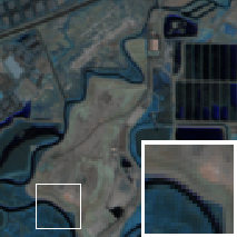
The Moffett Field [63] was acquired by Airborne Visible/Infrared Imaging Spectrometer (AVIRIS) over the urban and rural area in Moffett Field, CA, USA, with a spatial resolution of m. This image consists of spectral bands in the range of nm. After removing noisy bands, we used a sub-image of size (Fig. 6 (a)) for experiments in simulated noise cases.
The Salinas [64] was collected by AVIRIS over the field area in Salinas Valley, CA, USA, with a spatial resolution of m. This image consists of spectral bands in the range of nm. After removing noisy bands, we used a sub-image of size (Fig. 8 (a)) for experiments in simulated noise cases.
The Suwannee [65] acquired by AVIRIS over National Wildlife Reserves in the Gulf of Mexico with a spatial resolution of m. This image consists of spectral bands in the range of nm. We used a sub-image of size (Fig. 13 (a)) for experiments in real noise cases.
The Bats1 and Bats2 [66], which include hundreds of bats, were collected with three FLIR SC6000 thermal infrared cameras at a frame rate of Hz. For more detailed descriptions, see also [3, 67, 68]. We used denoised and raw sub-images of size (Figs. 7 (a) and 13 (b)) for experiments in simulated and real noise cases, respectively.
IV-C Experiments in Simulated Noise Cases
For the HSI destriping experiments, the parameter of each stripe noise characterization model summarized in Tab. II was set to a hand-optimized value, so as to achieve the best MPSNR. For fair comparison, we set to the oracle value, i.e., . As quantitative evaluations, we employed the mean peak signal-to-noise ratio (MPSNR):
| (28) |
and the mean structural similarity overall bands (MSSIM) [69]:
| (29) |
where is the th band of . The larger these values are, the better the destriping results are. The stopping criterion of Alg. 1 was set as .
We generated the three types of degraded images:
- (i)
HSIs with vertical stripe noise,
- (ii)
IR videos with time-invariant vertical stripe noise,
- (iii)
HSIs with vertical stripe noise and white Gaussian noise.
In the IR video experiments, we only consider stripe noise because Gaussian-like random noise does not appear in raw IR video data [14, 15]. For the variety of experiments, we considered the following five types of the intensity range of stripe noise: , , , , and . The standard deviation of white Gaussian noise was set to .
Tables IV, V, and VI list the resulting MPSNR and MSSIM values in Case (i), Case (ii), and Case (iii), respectively. The best and second-best values are highlighted in bold and underline, respectively. The proposed FC achieved the best/second-best MPSNR and MSSIM values in most cases. S and GS performed worse overall. LR and TV performed better than S and GS. However, the performance of LR and TV is significantly degraded in the cases where they are combined with a low-rank image regularization (LR-TNN) and TV image regularizations (TV-SSTV and TV-ASSTV), respectively.
Figures 6, 7, and 8 depict the Moffett field destriping results in Case (i) using SSTV, the Bats1 destriping results in Case (ii) using ATV, and the Salinas destriping results in Case (iii) using TNN, respectively. Figure 9 plots their band-wise or frame-wise PSNRs and SSIMs. In the 95th-band results of Figs. 9 (a) and (b), the PSNRs and SSIMs of S-SSTV, GS-SSTV, and LR-SSTV dropped to 30 [dB] and 0.7, respectively. This is because S-SSTV, GS-SSTV, and LR-SSTV excessively smoothened the spectral signatures around the band. In the magnified areas of Figs. 6 (c), (d), and (e), we see that the land shapes of the red and green bands are removed as Gaussian and stripe noise. TV-SSTV also resulted in the low PSNRs and SSIMs of the band 95 and eliminated some edges in addition to the stripe noise (see Fig. 6 (f)). S-ATV, GS-ATV, LR-ATV, and TV-ATV removed bats as stripe noise, resulting in poor performance (see Figs. 7 (c), (d), (e), and (f)). Figures 9 (c) and (d) show that the PSNRs and SSIMs of S-ATV, GS-ATV, LR-ATV, and TV-ATV vary according to frame numbers. The reason is that the results are worse as the number of unrestored bats increases. In contrast, FC-SSTV recovers the land shapes and edges (see Fig. 6 (f)) and FC-ATV accurately removed stripe noise, leading to high PSNRs and SSIMs. The SSIM results for Figs. 9 (e) and (f) were better for LR than FC and TV, but the PSNRs were better for FC and TV than LR. In particular, from 30 to 150 bands, FC and TV achieved [dB] better PSNRs and worse SSIMs than LR. In the magnified area of the stripe noise by LR-TNN (Fig. 8 (e)), the yellow line appears along with a field shape. This indicates that LR-TNN restores the image structure but does not recover the contrast. The three results verify that FC consistently achieves high performance due to its accurate capturing ability for stripe noise.
Figure 10 shows the means of MPSNRs and MSSIMs in each noise case. In Case (i), LR and FC accurately captured stripe noise, leading to better performances than TV. In Case (ii), FC achieved the best performance. This is because FC captures the temporal flatness while the other characterizations do not. In Case (iii), LR captured horizontal lines as a stripe noise component to remove Gaussian noise by the intersections between vertical stripe noise and the horizontal lines, leading to worse results. On the other hand, TV and FC obtained better results than LR without capturing the horizontal lines.
Figure 11 plots the means of MPSNRs and MSSIMs in each stripe noise intensity. LR dropped its MPSNRs as the stripe noise intensities increased. This is due to the fact that LR removes the meaningful image components as stripe noise components if stripe noise intensity is high. The MPSNRs and MSSIMs of TV did not decrease depending on the stripe noise intensities but were lower than FC overall. Compared with these existing stripe noise characterizations, FC accurately eliminated stripe noise, resulting in high destriping performances regardless of the stripe noise intensity.
Figure 12 shows the means of MPSNRs and MSSIMs in each image regularization. FC resulted in [dB] worse MPSNRs than LR for the ASSTV and SSTV+TNN cases. This is because FC-ASSTV and FC-SSTV+TNN stop the iterations before the stripe noise components satisfy the flatness constraint, leading to slightly dropping their MPSNRs and MSSIMs. On the other hand, FC did obtain a [dB] better MPSNR and better MSSIM than LR for the TNN case. Compared with TV, the performances of FC were similar for HTV, TNN, SSTV+TNN, and -HTV and better for SSTV and ASSTV. Moreover, FC stably performed better than the other characterizations for ATV, ITV, and ATV+NN. These reveal that our framework achieves good performance on average, whatever image regularizations are used.
IV-D Experiments in Real Noise Cases
In the real noise-case experiments, the parameter (Tab. II) for each method was determined manually to balance the tradeoff between the visual quality (e.g., over-smoothed or not) and destriping performance (e.g., stripe noise is sufficiently removed or not). For the data fidelity parameter , we adjusted it to an appropriate value after empirically estimating the intensity of the noise in the real data. Specifically, it was set to 200 for Suwannee and 0 for Bats2. The stopping criterion of Alg. 1 was set as .
We show the Suwannee destriping results for a real noise case in Fig. 14. The destriping result by S-HTV (Fig. 14 (a1)) includes residual stripe noise. The results by S-SSTV (Fig. 14 (a2)), GS-SSTV (Fig. 14 (b2)), S-ASSTV (Fig. 14 (a3)), GS-ASSTV (Fig. 14 (b3)), S-TNN (Fig. 14 (a4)), GS-TNN (Fig. 14 (b4)), and S--HTV (Fig. 14 (a6)) have brighter areas than the original image (Fig. 13 (a)), and some of the land shapes in the magnified areas were removed as the stripe noise components. These suggest that S and GS are less capable of capturing the vertical continuity of stripe noise. LR-ASSTV (Fig. 14 (c3)) recovered the narrow river that lies along with the vertical direction in the magnified areas. On the other hand, LR-SSTV (Fig. 14 (c2)) and LR-TNN (Fig. 14 (c4)) removed part of the global structure in the image as stripe noise. This may be due to the fact that LR allows for changes in the overall luminance level so that it does not prevent spectral oversmoothing caused by the image regularizations. In the results by TV-SSTV (Fig. 14 (d2)), TV-ASSTV (Fig. 14 (d3)), TV-SSTV+TNN (Fig. 14 (d5)), and TV--HTV (Fig. 14 (d6)), land shape was also partially removed as stripe noise. For example, TV-ASSTV (Fig. 14 (d3)) completely removed the narrow river in the magnified area. This is because there is a conflict between SSTV, ASSTV, SSTV+TNN, and -HTV, used as image regularizations, and TV, used as a stripe noise characterization. Compared with these existing stripe noise characterizations, for FC-HTV, FC-SSTV, FC-TNN, FC--HTV, its strong ability of stripe noise characterization allows us to achieve desirable destriping. However, our results do not satisfy the flatness constraint and slightly include land shapes in the stripe noise components only for FC-ASSTV and FC-SSTV+TNN (Figs. 14 (e3) and (e5)). This indicates that FC-ASSTV and FC-SSTV+TNN need more iterations to preclude the land shapes from their stripe noise components.
ATV
Estimated IR video


Stripe noise


(a1) S [29]
(b1) GS [37]
(c1) LR [40]
(d1) TV [44]
(e1) FC
ITV
Estimated IR video
Stripe noise

(a2) S [29]
(b2) GS [37]
(c2) LR [40]
(d2) TV [44]
(e2) FC
ATV+NN
Estimated IR video
Stripe noise

(a3) S [29]
(b3) GS [37]
(c3) LR [40]
(d3) TV [44]
(e3) FC
Figure 15 shows the destriping results of the IR video Bats2. S and TV removed bats (moving objects) as stripe noise. This is because the stripe noise components (Figs. 15 (a1), (a2), (a3), (d1), (d2), and (d3)) have sparse or vertical smoothness properties. GS and LR performed better than S and TV, but some of bats were regarded as stripe noise components (see Figs. 15 (b1), (b2), (b3), (c1), (c2), and (c3)). In contrast to these stripe noise characterizations, our FC, when combined with any of the image regularizations, removed only the stripe noise while maintaining bats (see Figs. 15 (e1), (e2), and (e3)).


(a)
(b)
(c)
(MPSNR, MSSIM)
(20.03, 0.5271)
(35.80, 0.8972)


(d)
(e)
(f)
(MPSNR, MSSIM)
(23.71, 0.8059)
(36.92, 0.9474)
IV-E Comparison With A Deep Learning-Based Method
We compare our framework with a deep learning-based method [20] 66 6 The code is available at https://github.com/acecreamu/deep-hs-prior., where we adjust the parameter so as to achieve the best MPSNR. As observed images, the Moffett Field and Salinas degraded by stripe noise with and Gaussian noise with are used. Figure 16 shows the destriping results, which validate the effectiveness of our framework compared to a deep learning-based method. The method in [20] did not recover edges and objects (Figs. 16 (b) and (e)), leading to worse MPSNRs and MSSIMs. This is due to the limitation of deep learning-based methods in capturing textures and singular features, as also mentioned in [21, 22].
IV-F Discussion
From the above experiments, we summarize the advantages and limitations of our framework as follows:
- •
FC accurately captures various intensities of stripe noise for any target images without image components.
- •
In particular, FC eliminates high intensities of stripe noise.
- •
Our framework consistently removes stripe noise, whatever image regularizations are combined.
- •
When using some image regularization such as ASSTV and SSTV+TNN, our framework requires many iterations to converge.
V Conclusion
In this paper, we have proposed a general destriping framework for remote sensing images. Specifically, we formulated the destriping as a convex optimization problem equipped with the flatness constraint. Thanks to the strong characterization of stripe noise, our framework is compatible with various regularization functions and achieves effective destriping. Then, we develop a solver for the problem based on DP-PDS, which allows us to avoid stepsize adjustment. Through destriping experiments using HSI and IR video data, we found that our framework is advantageous on average compared to existing methods, whatever image regularizations are used. For future work, our framework needs the extension to consider the various degradation such as the spectral variability and the effectiveness demonstration in remote sensing image applications such as classification, unmixing, compressed sensing reconstruction, and target recognition.
Appendix A Convergence of DP-PDS
Consider a convex optimization problem of the following form:
| (30) |
where and are variables that include tensors and tensors, respectively, and are proper lower semi-continuous convex functions, and is a linear operator.
We consider the following iterative procedures:
| (31) |
where is the Fenchel–Rockafellar conjugate function of , and and are preconditioners. For any and , the sequence generated by (31) converges to the optimal solution of Prob. (30) if the linear operator and preconditioners satisfy the following condition [59, Lemma 1]: for any
| (32) |
Note that matrix-vector multiplication between a diagonal matrix and a vector is equivalent to tensor-tensor Hadamard product. Therefore, Eq. (31) is identical to the algorithm described in [59].
DP-PDS sets and as follows. Since is a linear operator, the th entry of is yielded by linear combinations of as follows:
| (33) |
Then, the th entry of is given as
| (34) |
Similarly, the th entry of is given as
| (35) |
Then, the th entry of is given as
| (36) |
These preconditioners and satisfy the condition in [59, Lemma 2], i.e., Eq. (31) computes the solution of Prob. (30).
Appendix B Convergence of our Algorithm
References
- [1] J. M. Bioucas-Dias, A. Plaza, N. Dobigeon, M. Parente, Q. Du, P. Gader, and J. Chanussot, “Hyperspectral unmixing overview: Geometrical, stastical, and sparse regression-based approaches,” IEEE J. Sel. Topics Appl. Earth Observ. Remote Sens., vol. 5, no. 2, pp. 354–379, Apr. 2012.
- [2] J. W. Beletic, R. Blank, D. Gulbransen, D. Lee, M. Loose, E. C. Piquette, T. Sprafke, W. E. Tennant, M. Zandian, and J. Zino, “Teledyne Imaging Sensors: infrared imaging technologies for astronomy and civil space,” in Proc. SPIE, vol. 7021, Jul. 2008, pp. 70 210H–1–14.
- [3] Z. Wu, N. Fuller, D. Theriault, and M. Betke, “A thermal infrared video benchmark for visual analysis,” in Proc. IEEE Conf. Comput. Vis. Pattern Recognit. (CVPR). IEEE, Jun.
- [4] W. He, H. Zhang, H. Shen, and L. Zhang, “Hyperspectral image denoising using local low-rank matrix recovery and global spatial–spectral total variation,” IEEE J. Sel. Topics Appl. Earth Observ. Remote Sens., vol. 11, no. 3, pp. 713–729, Mar. 2018.
- [5] N. Liu, W. Li, R. Tao, and J. E. Fowler, “Wavelet-domain low-rank/group-sparse destriping for hyperspectral imagery,” IEEE Trans. Geosci. Remote Sens., vol. 57, no. 12, pp. 10 310–10 321, Dec. 2019.
- [6] L. Liu, L. Xu, and H. Fang, “Simultaneous intensity bias estimation and stripe noise removal in infrared images using the global and local sparsity constraints,” IEEE Trans. Geosci. Remote Sens., vol. 58, no. 3, pp. 1777–1789, Mar. 2020.
- [7] W. Ma, J. M. Bioucas-Dias, T.-H. Chan, N. Gillis, P. Gader, A. J. Plaza, A. Ambikapathi, and C. Chi, “A signal processing perspective on hyperspectral unmixing: Insights from remote sensing,” IEEE Signal Process. Mag., vol. 31, no. 1, pp. 67–81, Jan. 2014.
- [8] A. Romero, C. Gatta, and G. Camps-Valls, “Unsupervised deep feature extraction for remote sensing image classification,” IEEE Trans. Geosci. Remote Sens., vol. 54, no. 3, pp. 1349–1362, Mar. 2016.
- [9] E. Maggiori, Y. Tarabalka, G. Charpiat, and P. Alliez, “Convolutional neural networks for large-scale remote-sensing image classification,” IEEE Trans. Geosci. Remote Sens., vol. 55, no. 2, pp. 645–657, Feb. 2017.
- [10] L. Gao, B. Zhao, X. Jia, W. Liao, and B. Zhang, “Optimized kernel minimum noise fraction transformation for hyperspectral image classification,” Remote Sensing, vol. 9, no. 6, Apr. 2017.
- [11] D. Hong, L. Gao, J. Yao, B. Zhang, A. Plaza, and J. Chanussot, “Graph convolutional networks for hyperspectral image classification,” IEEE Trans. Geosci. Remote Sens., vol. 59, no. 7, pp. 5966–5978, Jul. 2021.
- [12] X. Li, V. Monga, and A. Mahalanobis, “Multiview automatic target recognition for infrared imagery using collaborative sparse priors,” IEEE Trans. Geosci. Remote Sens., vol. 58, no. 10, pp. 6776–6790, Oct. 2020.
- [13] B. Munch, P. Trtik, F. Marone, and M. Stampanoni, “Stripe and ring artifact removal with combined wavelet-fourier filtering,” Opt. Express, vol. 17, no. 10, pp. 8567–8591, May 2009.
- [14] R. Sheng-Hui, Z. Hui-Xin, Q. Han-Lin, L. Rui, and Q. Kun, “Guided filter and adaptive learning rate based non-uniformity correction algorithm for infrared focal plane array,” Infr. Phys. Technol., vol. 76, pp. 691–697, May 2016.
- [15] Q. Zeng, H. Qin, X. Yan, and H. Zhou, “Fourier spectrum guidance for stripe noise removal in thermal infrared imagery,” IEEE Geosci. Remote Sens. Lett., vol. 17, no. 6, pp. 1072–1076, Jun. 2020.
- [16] X. Kuang, X. Sui, Y. Liu, Q. Chen, and G. Gu, “Single infrared image optical noise removal using deep convolutional networks,” IEEE Photon. J., vol. 10, no. 2, pp. 1–15, Apr. 2018.
- [17] Y. Chang, L. Yan, L. Liu, H. Fang, and S. Zhong, “Infrared aerothermal nonuniform correction via deep multiscale residual network,” IEEE Geosci. Remote Sens. Lett., vol. 16, no. 7, pp. 1120–1124, Jul. 2019.
- [18] Y. Chang, L. Yan, H. Fang, S. Zhong, and W. Liao, “Hsi-denet: Hyperspectral image restoration via convolutional neural network,” IEEE Trans. Geosci. Remote Sens., vol. 57, no. 2, pp. 667–682, Feb. 2019.
- [19] J. Song, J.-H. Jeong, D.-S. Park, H.-H. Kim, D.-C. Seo, and J.-C. Ye, “Unsupervised denoising for satellite imagery using wavelet directional cyclegan,” IEEE Trans. Geosci. Remote Sens., vol. 59, no. 8, pp. 6823–6839, Aug. 2021.
- [20] O. Sidorov and J. Y. Hardeberg, “Deep hyperspectral prior: Single-image denoising, inpainting, super-resolution,” in Proc. IEEE/CVF Int. Conf. Comput. Vis. (ICCV), Oct. 2019, pp. 3844–3851.
- [21] P. Liu, M. Wang, L. Wang, and W. Han, “Remote-sensing image denoising with multi-sourced information,” IEEE J. Sel. Topics Appl. Earth Observ. Remote Sens., vol. 12, no. 2, pp. 660–674, Feb. 2019.
- [22] T.-X. Jiang, L. Zhuang, T.-Z. Huang, X.-L. Zhao, and J. M. Bioucas-Dias, “Adaptive hyperspectral mixed noise removal,” IEEE Trans. Geosci. Remote Sens., early access, vol. 60, Jun. 2021, Art no. 5511413, doi: 10.1109/TGRS.2021.3085779.
- [23] Q. Yuan, L. Zhang, and H. Shen, “Hyperspectral image denoising employing a spectral-spatial adaptive total variation model,” IEEE Trans. Geosci. Remote Sens., vol. 50, no. 10, pp. 3660–3677, Oct. 2012.
- [24] H. K. Aggarwal and A. Majumdar, “Hyperspectral image denoising using spatio-spectral total variation,” IEEE Geosci. Remote Sens. Lett., vol. 13, no. 3, pp. 442–446, Mar. 2016.
- [25] Y. Chang, L. Yan, H. Fang, and C. Luo, “Anisotropic spectral-spatial total variation model for multispectral remote sensing image destriping,” IEEE Trans. Image Process., vol. 24, no. 6, pp. 1852–1866, Jun. 2015.
- [26] Y. Chen, H. T.-Z, X.-L. Zhao, L.-J. Deng, and J. Huang, “Stripe noise removal of remote sensing images by total variation regularization and group sparsity constraint,” Remote Sens., vol. 9, no. 6, p. 559, Jun. 2017.
- [27] M. Wang, Q. Wang, J. Chanussot, and D. Hong, “- hybrid total variation regularization and its applications on hyperspectral image mixed noise removal and compressed sensing,” IEEE Trans. Geosci. Remote Sens., vol. 59, no. 9, pp. 7695–7710, Sep. 2021.
- [28] S. H. Chan, R. Khoshabeh, K. B. Gibson, P. E. Gill, and T. Q. Nguyen, “An augmented lagrangian method for total variation video restoration,” IEEE Trans. Image Process., vol. 20, no. 11, pp. 3097–3111, Nov. 2011.
- [29] H. Zhang, W. He, L. Zhang, H. Shen, and Q. Yuan, “Hyperspectral image restoration using low-rank matrix recovery,” IEEE Trans. Geosci. Remote Sens., vol. 52, no. 8, pp. 4729–4743, Aug. 2014.
- [30] H. Fan, Y. Chen, H. Zhang, and G. Kuang, “Hyperspectral image restoration using low-rank tensor recovery,” IEEE J. Sel. Topics Appl. Earth Observ. Remote Sens., vol. 10, no. 10, pp. 4589–4604, Oct. 2017.
- [31] Y. Chen, Y. Guo, Y. Wang, D. Wang, C. Peng, and G. He, “Denoising of hyperspectral images using nonconvex low rank matrix approximation,” IEEE Trans. Geosci. Remote Sens., vol. 55, no. 9, pp. 5366–5380, Sep. 2017.
- [32] H. Ye, H. Li, B. Yang, F. Cao, and Y. Tang, “A novel rank approximation method for mixture noise removal of hyperspectral images,” IEEE Trans. Geosci. Remote Sens., vol. 57, no. 7, pp. 4457–4469, 2019.
- [33] Y.-B. Zheng, T.-Z. Huang, X.-L. Zhao, T.-X. Jiang, T.-H. Ma, and T.-Y. Ji, “Mixed noise removal in hyperspectral image via low-fibered-rank regularization,” IEEE Trans. Geosci. Remote Sens., vol. 58, no. 1, pp. 734–749, Jan. 2020.
- [34] J. Xue, Y. Zhao, W. Liao, and J. C. Chan, “Nonlocal low-rank regularized tensor decomposition for hyperspectral image denoising,” IEEE Trans. Geosci. Remote Sens., vol. 57, no. 7, pp. 5174–5189, Jul. 2019.
- [35] H. Shen, X. Li, L. Zhang, D. Tao, and C. Zeng, “Compressed sensing-based inpainting of aqua moderate resolution imaging spectroradiometer band 6 using adaptive spectrum-weighted sparse bayesian dictionary learning,” IEEE Trans. Geosci. Remote Sens., vol. 52, no. 2, pp. 894–906, Feb. 2014.
- [36] Y. Wang, Y. Y. Tang, C. Zou, and L. Yang, “Spectral-spatial hyperspectral image destriping using sparse learning and spatial unidirection prior,” in Proc. IEEE Int. Conf. Cybern. (CYBCONF), Jul. 2017, pp. 1–5.
- [37] T. Ince, “Hyperspectral image denoising using group low-rank and spatial-spectral total variation,” IEEE Access, vol. 7, pp. 52 095–52 109, Apr. 2019.
- [38] H. Fan, C. Li, Y. Guo, G. Kuang, and J. Ma, “Spatial-spectral total variation regularized low-rank tensor decomposition for hyperspectral image denoising,” IEEE Trans. Geosci. Remote Sens., vol. 56, no. 10, pp. 6196–6213, Oct. 2018.
- [39] Y. Chen, T.-Z. Huang, L.-J. Deng, X.-L. Zhao, and M. Wang, “Group sparsity based regularization model for remote sensing image stripe noise removal,” Neurocomput., vol. 267, no. 6, pp. 95–106, Dec. 2017.
- [40] Y. Chang, L. Yan, T. Wu, and S. Zhong, “Remote sensing image stripe noise removal: From image decomposition perspective,” IEEE Trans. Geosci. Remote Sens., vol. 54, no. 12, pp. 7018–7031, Dec. 2016.
- [41] T. Hu, W. Li, N. Liu, R. Tao, F. Zhang, and P. Scheunders, “Hyperspectral image restoration using adaptive anisotropy total variation and nuclear norms,” IEEE Trans. Geosci. Remote Sens., vol. 59, no. 2, pp. 1516–1533, Feb. 2021.
- [42] X. Liu, X. Lu, H. Shen, Q. Yuan, Y. Jiao, and L. Zhang, “Stripe noise separation and removal in remote sensing images by consideration of the global sparsity and local variational properties,” IEEE Trans. Geosci. Remote Sens., vol. 54, no. 5, pp. 3049–3060, May 2016.
- [43] X. Liu, H. Shen, Q. Yuan, X. Lu, and C. Zhou, “A universal destriping framework combining 1-D and 2-D variational optimization methods,” IEEE Trans. Geosci. Remote Sens., vol. 56, no. 2, pp. 808–822, Feb. 2018.
- [44] H.-X. Dou, T.-Z. Huang, L.-J. Deng, X.-L. Zhao, and J. Huang, “Directional l0 sparse modeling for image stripe noise removal,” Remote Sensing, vol. 10, no. 3, p. 361, Feb. 2018.
- [45] R. Chartrand, “Nonconvex splitting for regularized low-rank + sparse decomposition,” IEEE Trans. Signal Process., vol. 60, no. 11, pp. 5810–5819, Nov. 2012.
- [46] B. E. Moore, C. Gao, and R. R. Nadakuditi, “Panoramic robust pca for foreground–background separation on noisy, free-motion camera video,” IEEE Trans. Comput. Imag., vol. 5, no. 2, pp. 195–211, Jun. 2019.
- [47] A. J. Tom and S. N. George, “Video completion and simultaneous moving object detection for extreme surveillance environments,” IEEE Signal Process. Lett., vol. 26, no. 4, pp. 577–581, Apr. 2019.
- [48] Q. Lu, Z. Lu, X. Tao, and H. Li, “A new non-local video denoising scheme using low-rank representation and total variation regularization,” in 2014 IEEE International Symposium on Circuits and Systems (ISCAS), Jun. 2014, pp. 2724–2727.
- [49] O. Riou, S. Berrebi, and P. Bremond, “Nonuniformity correction and thermal drift compensation of thermal infrared camera,” in Proc. SPOE, Thermosense XXVI, vol. 5405, Apr. 2004, pp. 294–302.
- [50] Y. Cao, M. Y. Yang, and C.-L. Tisse, “Effective strip noise removal for low-textured infrared images based on 1-d guided filtering,” IEEE Trans. Circuits Syst. Video Technol., vol. 26, no. 12, pp. 2176–2188, Dec. 2016.
- [51] N. D. Sidiropoulos, L. D. Lathauwer, X. Fu, K. Huang, E. E. Papalexakis, and C. Faloutsos, “Tensor decomposition for signal processing and machine learning,” IEEE Trans. Signal Process., vol. 65, no. 13, pp. 3551–3582, Jul 2017.
- [52] Y. Ji, Q. Wang, X. Li, and J. Liu, “A survey on tensor techniques and applications in machine learning,” IEEE Access, vol. 7, pp. 162 950–162 990, 2019.
- [53] K. Naganuma, S. Takeyama, and S. Ono, “Zero-gradient constraints for destriping of remote-sensing data,” in 2021 IEEE International Conference on Acoustics, Speech and Signal Processing (ICASSP), Jun. 2021.
- [54] M. Afonso, J. Bioucas-Dias, and M. Figueiredo, “An augmented Lagrangian approach to the constrained optimization formulation of imaging inverse problems,” IEEE Trans. Image Process., vol. 20, no. 3, pp. 681–695, Mar. 2011.
- [55] M. Carlavan and L. Blanc-Féraud, “Sparse Poisson noisy image deblurring,” IEEE Trans. Image Process., vol. 21, no. 4, pp. 1834–1846, Apr. 2012.
- [56] G. Chierchia, N. Pustelnik, J.-C. Pesquet, and B. Pesquet-Popescu, “Epigraphical projection and proximal tools for solving constrained convex optimization problems,” Signal, Image Video Process., vol. 9, no. 8, pp. 1737–1749, 2015.
- [57] S. Ono and I. Yamada, “Signal recovery with certain involved convex data-fidelity constraints,” IEEE Trans. Signal Process., vol. 63, no. 22, pp. 6149–6163, Nov. 2015.
- [58] S. Ono, “Efficient constrained signal reconstruction by randomized epigraphical projection,” in Proc. IEEE Int. Conf. Acoust., Speech, Signal Process. (ICASSP). IEEE, 2019, pp. 4993–4997.
- [59] T. Pock and A. Chambolle, “Diagonal preconditioning for first order primal-dual algorithms in convex optimization,” in Proc. IEEE Int. Conf. Comput. Vis. (ICCV), Nov. 2011, pp. 1762–1769.
- [60] A. Chambolle and T. Pock, “A first-order primal-dual algorithm for convex problems with applications to imaging,” J. Math. Imag. Vis., vol. 40, no. 1, pp. 120–145, 2011.
- [61] L. Condat, “A primal-dual splitting method for convex optimization involving lipschitzian, proximable and linear composite terms,” J. Opt. Theory Appl., vol. 158, no. 2, pp. 460–479, 2013.
- [62] S. Becker and J. Fadili, “A quasi-newton proximal splitting method,” in Proc. Adv. Neural Inf. Process Syst., 2012, pp. 2618–2626.
- [63] “AVIRIS,” https://aviris.jpl.nasa.gov/data/free_data.html.
- [64] “GIC,” http://www.ehu.eus/ccwintco/index.php?title=Hyperspectral_Remote_Sensing_Scenes.
- [65] “SpecTIR,” http://www.spectir.com/free-data-samples/.
- [66] “BU-TIV Dataset,” http://csr.bu.edu/BU-TIV/BUTIV.html.
- [67] Z. Wu, N. I. Hristov, T. H. Kunz, and M. Betke, “Tracking-reconstruction or reconstruction-tracking? comparison of two multiple hypothesis tracking approaches to interpret 3d object motion from several camera views,” in Proc. Workshop Motion Video Comput. (WMVC), Dec. 2009, pp. 1–8.
- [68] Z. Wu, A. Thangali, S. Sclaroff, and M. Betke, “Coupling detection and data association for multiple object tracking,” in Proc. IEEE Conf. Comput. Vis. Pattern Recognit. (CVPR), Jun. 2012, pp. 1948–1955.
- [69] Z. Wang, A. C. Bovik, H. R. Sheikh, and E. P. Simoncelli, “Image quality assessment: from error visibility to structural similarity,” IEEE Trans. Image Process., vol. 13, no. 4, pp. 600–612, Apr. 2004.
![[Uncaptioned image]](2104.02845v4/naganuma.JPG) |
Kazuki Naganuma (S’21) received a B.E. degrees in Information and Computer Sciences in 2020 from the Kanagawa Institute of Technology. He is currently pursuing an M.E. degree at the Department of Computer Science in the Tokyo Institute of Technology. His current research interests are in signal and image processing and optimization theory. |
![[Uncaptioned image]](2104.02845v4/prof_ono_book_bio.jpg) |
Shunsuke Ono (S’11–M’15) received a B.E. degree in Computer Science in 2010 and M.E. and Ph.D. degrees in communications and computer engineering in 2012 and 2014 from the Tokyo Institute of Technology, respectively. From April 2012 to September 2014, he was a Research Fellow (DC1) of the Japan Society for the Promotion of Science (JSPS). He is currently an Associate Professor in the Department of Computer Science, School of Computing, Tokyo Institute of Technology. From October 2016 to March 2020, he was a Researcher of Precursory Research for Embryonic Science and Technology (PRESTO), Japan Science and Technology Corporation (JST), Tokyo, Japan. His research interests include signal processing, computational imaging, hyperspectral imaging and fusion, mathematical optimization, and data science. Dr. Ono received the Young Researchers’ Award and the Excellent Paper Award from the IEICE in 2013 and 2014, respectively, the Outstanding Student Journal Paper Award and the Young Author Best Paper Award from the IEEE SPS Japan Chapter in 2014 and 2020, respectively, and the Funai Research Award from the Funai Foundation in 2017. He has been an Associate Editor of IEEE TRANSACTIONS ON SIGNAL AND INFORMATION PROCESSING OVER NETWORKS since 2019. |