, yongxiao@hust.edu.cn, krunz@arizona.edu
Misbehavior Detection in Wi-Fi/LTE Coexistence over Unlicensed BandsAn abridged version of this paper appeared in the Proc. of the 11th ACM Conference on Security and Privacy in Wireless and Mobile Networks (Wisec), 2018, [1].
Abstract
We consider the problem of fair coexistence between LTE and Wi-Fi systems in the unlicensed 5 GHz U-NII bands. We focus on the misbehavior opportunities due to the heterogeneity in channel access mechanism and the lack of a common control plane. We define selfish misbehavior strategies for the LTE that yield an unfair share of the spectrum resources. Such strategies are based on manipulating the operational parameters of the LTE-LAA standard, namely the backoff mechanism, the traffic class parameters, the clear channel access (CCA) threshold, and others. Prior methods for detecting misbehavior in homogeneous settings are not applicable in a spectrum sharing scenario because the devices of one system cannot decode the transmissions of another. We develop implicit sensing techniques that can accurately estimate the operational parameters of LTE transmissions under various topological scenarios and without decoding. These techniques apply correlation-based signal detection to infer the required information. Our techniques are validated through experiments on a USRP testbed. We further apply a statistical inference framework for determining deviations of the LTE behavior from the coexistence etiquette. By characterizing the detection and false alarm probabilities, we show that our framework yields high detection accuracy at a very low false alarm rate. Although our methods focus on detecting misbehavior of the LTE system, they can be generalized to other coexistence scenarios.
I Introduction
The high demand for wireless services has fueled a severe shortage in radio spectrum resources. The regulatory approach for meeting this galloping demand is to allow the coexistence of competing wireless technologies in common bands. An example of such coexistence is that of LTE and Wi-Fi in the 5 GHz U-NII band [2, 3, 4, 5, 6]. However, shared spectrum introduces novel challenges for the secure, efficient, and fair channel access. Many of these challenges arise from the heterogeneity of the coexisting systems, the system scale, and the lack of explicit coordination mechanisms between them. Such heterogeneity is manifested in different PHY-layer capabilities, channel access dynamics (dynamic vs. fixed), schedule-based vs. random access, interference-avoiding vs. interference-mitigating, etc. Altogether, this creates a complex coexistence scenario without a unified control plane.
Several recent efforts have addressed the problem of fair coexistence of LTE/Wi-Fi and Wi-Fi/Zigbee under benign settings (e.g., [7, 8, 9, 10, 11, 12, 13, 14, 15, 16, 17, 18, 19, 20, 21, 22]). Recent analytical and experimental studies have shown that an LTE system could cause serious performance degradation to a co-present Wi-Fi system, even if the LTE remains protocol-compliant [23, 24]. The main approach to address unfair channel access is to introduce the Licensed-Assisted Access (LAA) protocol that follows the Listen-Before-Talk (LBT) mechanism [25]. Tao et al. showed that dynamically adjusting the contention window (CW) size can be beneficial for fair coexistence [26]. Follow-up works achieved further improvements by controlling other protocol parameters and applying other enhancements, e.g., [27, 28, 29, 30, 31].
Intentional violations of the coexistence etiquette to gain an unfair spectrum share have not been studied at length. Ying et al. were among the first to consider the problem of misbehavior when cycle-based LTE-U and Wi-Fi coexist [32]. The authors recognized that because the LTE duty cycle is unilaterally controlled by the LTE system, it can be abused to increase LTE’s spectrum share. They proposed a monitoring mechanism that accurately estimates the duty cycle and allows a spectrum manager to detect any misbehavior. The proposed scheme is not applicable to LTE-LAA, which is embraced by most operators and the standardization bodies [25]. In this paper, we focus on misbehavior detection mechanisms specific to the prevailing LTE-LAA standard.
Our methods build upon prior works on misbehavior detection for homogeneous networks, e.g., [33, 34, 35, 36, 37], with notable differences. First, heterogeneous networks do not share common coordination channels for communicating explicit control information such as the network allocation vector (NAV) field, device IDs, reservation messages (RTS/CTS), etc. Without explicit coordination, detecting the state and monitoring the behavior of stations operating under a different technology is challenging, as the messages exchanged by one system are undecodable at the other. Relevant challenges include determining which system occupies the channel, for how long, at what locality, with what range, and which stations collided, to name a few. Moreover, although the LTE-LAA and Wi-Fi standards follow the same carrier-sense multiple access (CSMA) approach, they adopt different channel contention parameters that affect the overall system behavior. Determining a system’s behavior requires accurate estimation of these parameters but using only implicit monitoring.
In this paper, we address the problem of misbehavior at the system level when heterogeneous technologies coexist. Specifically, we consider a misbehaving LTE-LAA system that coexists with Wi-Fi. LTE devices aim at occupying the shared spectrum for a longer fraction of time by manipulating the channel access mechanism of LAA. We propose a framework that detects LTE misbehavior, taking into account the absence of any means for explicit coordination. Our framework relies on implicit sensing mechanisms that provide accurate approximations of the operational parameters used by the misbehaving LTE devices. Our contributions are summarized as follows:
- •
We study the problem of channel access misbehavior of LTE-LAA when coexisting with Wi-Fi. Although possible misbehaving strategies bear resemblance to those in a homogeneous setting, we highlight novel challenges that stem from the technology heterogeneity and lack of explicit coordination.
- •
We introduce a new suite of monitoring mechanisms that do not rely on signal decoding for estimating relevant LTE-LAA protocol parameters. We develop implicit sensing techniques that go beyond simple LTE transmission detection to determine the presence of hidden stations, identify retransmitted frames, and specify the LTE priority class. These are essential parameters for accurately estimating the overall LTE behavior.
- •
We validate the effectiveness of the implicit parameter-estimation techniques in a USRP testbed. We show that these techniques are reliable and accurate.
- •
We propose a misbehavior detection mechanism based on statistical inference. This mechanism allows a monitor to detect any deviations of LTE behavior from the spectrum sharing etiquette.
- •
We investigate the detection performance under different traffic loads and adapt our framework accordingly to guarantee high detection and low false alarm probabilities.
- •
We perform extensive simulations to validate the proposed misbehavior detection mechanism and show that our approach yields near-perfect detection probability and a negligible false alarm rate.
The remainder of this paper is organized as follows. We discuss related works in Section II. The system and misbehavior models are introduced in Section III. The adopted implicit techniques for monitoring LTE activities are detailed in Section IV. In Section V, we demonstrate how the LTE channel access behavior can be accurately evaluated. We validate the performance of the proposed implicit techniques in Section VI. We analyze the detection scheme performance in Section VII and summarize the main contributions of this work in Section VIII.
II Background and Related work
II-A LTE-LAA Release 15
We consider an LTE system that follows the LAA specification, as described in Release 15 [25]. The standard defines four traffic priority classes. The first two classes are suitable for transmitting control messages and short frames, whereas classes and accommodate longer LTE frames.
Downlink channel access: The downlink channel access mechanism of LTE-LAA is shown in Fig. 1. Channel access parameters are listed in Table I and the channel access steps are as follows.
- 1.
Before transmitting a frame, the eNB freezes for an initial time consisting of a defer time plus observation slots, each of length . The parameter takes larger values for lower priority classes to compensate for the longer frame size. If the channel stays idle during , the eNB proceeds to the backoff phase described in Step 2, otherwise it repeats Step 1. The channel state (busy or idle) is determined by sensing the power on a given channel. If the power is less than the CCA threshold ( dBm according to [25]), for at least , the channel is inferred to be idle and it is busy, otherwise.
- 2.
The eNB initializes the backoff counter to a value uniformly selected in , where is the contention window (CW) size, initially set to a minimum value .
- 3.
The eNB decrements its backoff counter by one with every idle slot. If a slot is sensed busy, the eNB freezes its backoff counter until the channel becomes idle. The channel must remain idle for before the backoff countdown can be resumed.
- 4.
When the backoff counter becomes zero, the eNB transmits a frame with a maximum duration of . The eNB then waits for an ACK/NACK. If it receives an ACK, the transmission round is completed. Otherwise, the process is repeated from Step 1 by doubling the CW size, up to a .
Uplink channel access: To make an uplink transmission, a UE must receive an uplink (UL) grant permission from the eNB. The UL grant permission determines the access type that should be used by the UE. The standard specifies two candidate types.
- •
Type 1: The UE follows the same backoff process described for the downlink, but with slightly different parameters as shown in Table I.
- •
Type 2: The UE waits for the channel to be idle for 25 s and then accesses the channel without further contention.
From both the DL and the UL procedures, we note that the priority classes differ in both the defer time and allowed CW sizes. As will be shown later, these differences can be exploited by LTE devices to shorten the time between consecutive transmissions.
| Class | (slots) | (slots) | (ms) | (slots) |
| Downlink channel access | ||||
| or | ||||
| or | ||||
| Uplink channel access | ||||
| or | ||||
| or | ||||
II-B Related Work
LTE/Wi-Fi coexistence in a benign setting has been studied extensively [16, 17, 18, 19, 20, 21, 22] as well as [38] and the references therein. Ratasuk et al. [24] showed that LTE outperforms Wi-Fi by replacing one of the Wi-Fi deployments with an LTE cell and comparing the respective throughput. Hirzallah et al. [39] showed that different access protocols for Wi-Fi and LTE can cause an increased collision rate and latency for both systems. They suggested a CCA threshold adaptation mechanism to promote fairness. In [19], authors proposed a framework that allows nodes to adapt their CW sizes based on observed transmissions, ensuring they receive equal airtime. The idea of adapting the backoff parameters of LTE/Wi-Fi to achieve a fair coexistence was also studied in [27, 26, 28, 29, 30, 31]. However, these works assumed that all stations are trustful and protocol-compliant.
Misbehavior detection for channel access in homogeneous networks has been extensively studied, especially for IEEE 802.11 protocols (e.g., [34, 35, 40, 33, 36, 41]). In [33], the authors introduced modifications to the IEEE 802.11 protocol to simplify misbehavior detection and presented a penalty scheme for punishing selfish users. Li et al. used multiple backoff counter observations to calculate the probability that a monitored station remains protocol-compliant [36]. Misbehavior was detected by comparing this probability to a threshold. Considering a fair channel allocation [35], Tang et al. proposed a real-time misbehavior detection mechanism, which relies on an indicator function that represents the difference between the number of successful transmissions and the number of expected transmissions. Toledo et al. applied the Kolmogorov-Smirnov test to detect misbehavior from the number of idle slots between two transmissions [40]. As all stations follow the same protocol, misbehavior is detected if the idle slot distribution of a station differs from that of others.
Whereas there is a wealth of interest in channel access misbehavior for homogeneous networks, misbehavior between coexisting technologies is relatively new. The work closest to ours is reported in [32]. However, the authors considered the misbehavior in the CSAT-based LTE-U protocol, not LAA. They developed a method for estimating the LTE duty cycle by tracking LTE transmissions. The latter are identified based on the frame length, as LTE frames are typically longer than Wi-Fi frames. Possible LTE misbehavior is detected by a central node called the spectrum manager, which has prior knowledge of the permitted duty cycle for LTE. In this paper, we consider misbehavior under the LTE-LAA standard that implements a CSMA-like (LBT) channel access model and involves drastically different misbehavior actions and remedies. Our work is similar to that of [32] in that we also employ a central node, which we call as the hub, to analyze the LTE behavior. The pivotal difference between our work and misbehavior detection in homogeneous networks lies in the monitoring mechanisms for obtaining samples of behavior. All prior works rely on frame decoding to attribute transmissions to their originators. This is not generally possible between different technologies. Moreover, LTE and Wi-Fi systems execute channel access protocols with different parameters. For instance, the LTE-LAA backoff parameters depend on the priority class. Accurate estimation of the LTE behavior requires mechanisms for classifying frames according to their respective classes. Additional challenges stem from the heterogeneity in transmission and interference ranges. A Wi-Fi station may backoff in the presence of an LTE transmission, but the converse may not occur.
III Models and Framework Overview
III-A System Model
We consider LTE devices that coexist with Wi-Fi access points (APs) over the 5 GHz unlicensed band. The one-hop neighborhood set (other devices inside the interference range) of device is denoted by . LTE devices and Wi-Fi APs may transmit at different powers, so does not imply that . As an example, in Fig. 2, AP is in the interference range of LTE (solid line), but LTE is not in the interference range of (dashed line). The transmission powers of the LTE and Wi-Fi are denoted by and , respectively. LTE devices and Wi-Fi terminals are considered to follow the LTE-LAA and IEEE 802.11ac standards, respectively.
We consider the misbehavior of one or more LTE devices which are monitored by any AP in their vicinity. The monitoring APs are capable of performing simple signal operations on RF signals like sampling and correlation. LTE-related observations are collected by APs and analyzed at a central hub. This could be achieved through a cloud service that allows the uploading of all observations made by the APs to a central repository. Such scenario is relevant in enterprise networks where multiple APs are under a single administrative control or can be offered as an overlay service to which APs subscribe. This assumption also helps us identify if misbehavior is detectable at the system level, given all distributed observations.
We initially focus on detecting the LTE misbehavior in backlogged conditions. Under such conditions, gains in performance due to LTE misbehavior occur at the expense of the Wi-Fi system. We later consider the detection of LTE misbehavior under unsaturated traffic conditions.

III-B Misbehavior Model
The goal of a misbehaving LTE is to capture the channel more frequently and for a longer time than competing APs. This can be achieved by manipulating the LAA protocol parameters in the uplink or downlink direction.
Misbehavior in the downlink direction. This is the most beneficial type of misbehavior because the downlink direction carries a far higher traffic volume than the uplink one and the eNB nodes transmit to a large number of LTE devices. An eNB node can misbehave in the following ways.
1) Decrease the defer time : An LTE device can reduce the defer time to initiate the backoff countdown process faster. It can select a defer time that belongs to a high priority class and transmit a frame of low priority class with longer duration. Alternatively, the LTE can completely ignore the defer time and initiate the backoff countdown immediately within a transmission round.
2) Increase the CCA threshold: Another manipulation strategy is to avoid freezing the backoff counter in the presence of active Wi-Fi APs. This leads to faster acquisition of the medium, which can be beneficial if a high-power eNB transmission overshadows Wi-Fi transmissions. Note that avoiding backoff freezing can occur in benign settings due to hidden terminals or due to power asymmetry. This is illustrated in Fig. 2. Assume that Wi-Fi AP acts as a monitor for the behavior of LTE , which is outside the interference range of AP (hidden terminal) and therefore does not freeze its backoff counter when AP transmits. This behavior may be perceived by AP , which is within the interference range of LTE , as misbehavior. In another scenario, AP observes that LTE does not freeze its backoff window when AP is active. This could be due to the transmission power asymmetry or due to misbehavior.
3) Reduce the backoff window: An LTE system can manipulate the LAA backoff process by selecting its backoff counter from a smaller window range , where . The value of may be selected from a high-priority class so that the LTE appears to be protocol-compliant. Moreover, LTE can avoid increasing its CW size after a collision, to reduce the delay between two consecutive channel access attempts. This can be done by simply ignoring any mandated doubling of the CW size after a collision or by taking advantage of the low CW sizes allowed for high-priority classes. Here, we consider a general model in which the LTE remains protocol-compliant for a fraction of time , while it uses a smaller CW of size for the remaining time. As an example of backoff manipulation, the LTE device can consistently select backoff values in the range , irrespective of the priority class. Moreover, in the event of successive collisions, it can maintain . Essentially, all priority classes are treated as if they were of . We emphasize that there is an inherent difficulty in attributing collisions to a transmitting device because: (a) collisions are receiver-dependent, and (b) in a heterogeneous setting, one system cannot decode the transmissions of other systems. Hence, detecting misbehavior that involves collisions is challenging.

Misbehavior in the uplink direction. Unlike DL transmissions, any UL transmission must be preceded by an UL grant permission from the eNB. This grant specifies the subframe where the UL transmission should start. Once the UL grant is received, the UE starts the backoff process. Here, the misbehavior strategies described for the DL direction are possible. However, they have limited benefit for the UE because a failure to seize the channel for a Type 1 transmission will lead to a much more aggressive channel access strategy for the next subframe (Type 2).
If the UE cannot complete the backoff process before the beginning of the allocated subframe due to contention (case 2 in Fig. 3), the UE is allowed to access the channel in the following subframe by only deferring for an initial time , where That is, the UE senses the channel for minimal time and does not follow a backoff process, thus increasing the chances of capturing the channel substantially.
Given the significantly higher volume of DL traffic, the requirement for a DL frame to schedule an UL transmission, and the aggressive channel access strategy of UL Type 2 transmissions, we only focus on detecting LTE misbehavior in the DL direction.
III-C Misbehavior Detection Framework Overview
To detect misbehaving eNBs, we propose a detection framework which consists of a behavior monitoring phase and a behavior evaluation phase, as shown in Fig. 4. During the behavior monitoring phase, monitoring APs listen to the wireless medium when they do not transmit. Each monitoring AP overhears LTE frames and infers behavior-related parameters such as the start and end times of the LTE frame, the transmitting eNB, the retransmission round, the traffic class, and the topological relation of the AP to the LTE (whether the AP is a hidden terminal to the transmitting LTE or not). All parameters are implicitly estimated without decoding LTE frames. Monitoring APs periodically report a time series of observations along with a time series of their own activity to a central hub for further processing.
In the behavior evaluation phase, the hub processes the information reported by the distributed network of APs to derive the channel access pattern of each monitored eNB. If the access pattern is deemed to deviate from the LAA specifications, the LTE system is considered misbehaving.

IV Behavior Monitoring Phase
The key challenge in monitoring the LTE behavior is the system heterogeneity. The monitoring APs cannot decode LTE transmissions as they may not be equipped with LTE receivers. In this section, we present several techniques for the implicit estimation of the LTE operating parameters. Specifically, each monitoring AP listens to the wireless medium when it is not active. Upon detection of channel activity that is not Wi-Fi decodable, it processes the signal without decoding to determine if it belongs to an LTE. For the detected LTE transmission, the AP estimates an observation vector of six parameters
| (1) |
where and denote the start and end times of the transmission, respectively, denotes an eNB identity, denotes the LTE traffic class, denotes the retransmission round, and is a flag that denotes if the monitoring AP belongs to the one-hop neighborhood of the transmitting LTE. In the remainder of the section, we describe this parameter estimation.
IV-A Detecting LTE Transmissions
The first step for estimating the LTE operating parameters is to determine when and for how long eNBs transmit. This allows the estimation of and To detect LTE transmissions, we adopt the cyclic prefix (CP)-based method proposed in [39]. Like any OFDM modulated signal, LTE transmissions utilize the CP concept to mitigate inter-symbol interference. The end of an OFDM symbol is appended at the beginning, forming the CP. In Fig. 5, CP1 is equal to D1, CP2 is equal to D2, etc.

A Wi-Fi AP can attribute a signal to an eNB by verifying that the CP and its copy are samples away, where and denote the lengths, in samples, of the LTE symbol and the CP, respectively. The duration of the LTE OFDM symbol, and consequently the appended CP, are fixed to unique values in the LTE standard [25]. Based on the fixed duration and the sampling rate, the AP determines the values of and . The main idea of this method is to detect high signal correlation when the CP samples are correlated to the end of the LTE symbol.
Algorithm 1: LTE transmission detection
Step 1: The AP samples the received signal.
Step 2: The AP fixes two time windows and of length , separated by samples. Then, it shifts the two windows simultaneously by one sample at a time while keeping the window separation fixed to .
Step 3: For each shift , the AP obtains the vectors of signal samples and that correspond to windows and (each of length ) and computes
| (2) |
where is the correlation between and ,
| (3) |
Here, is the complex conjugate of . The energies and are computed as
| (4) |
| (5) |
We use the max in the denominator to ensure that always stays within and to help minimize the value of when and are different.
Step 4: If , the correlation spikes indicating that is the CP of . The correlation spike is recognized if where is a minimum correlation threshold that defines a signal match. We discuss the selection of the threshold in Section VI-B.
Step 5: The AP sets to the time of the first local maximum (correlation spike) that exceeds and to the time of the last local maximum that exceeds .
IV-B Differentiating Between eNBs
Attributing transmissions to individual eNBs is necessary for building the behavioral profile of each eNB. However, this requires: (a) to distinguish downlink LTE transmissions from uplink ones and (b) differentiate between eNBs in the downlink.
To perform these two operations, we propose that monitoring APs use two distinct frame fields included only in the DL direction. Those are the primary synchronization signal (PSS) and the secondary synchronization signal (SSS), which are used for synchronization and carry information about the transmitting eNB’s identity. As shown in Fig. 6, the PSS and SSS fields are repeated twice at fixed locations in an LTE DL frame. Samples of DL LTE signals at those fixed locations are identical. This gives the opportunity to a monitoring AP to identify DL frames.

Moreover, the identity of an eNB is calculated as ID , where and define the physical-layer cell identity group and physical layer identity of the LTE, respectively. The and values are part of the PSS and SSS fields. The pair is unique for every eNB, however, both can only be obtained by decoding the PSS and SSS fields.
Monitoring APs can exploit the known locations for and to attribute LTE transmissions to different eNBs. Note that we are not interested in extracting the ID value, but to identify LTE frames with the same ID. We use the “signal signature” of the static PSS and SSS fields for this attribution. The main idea is to detect the unique fields by sampling the LTE transmission at the PSS and SSS locations and correlating the signal samples with previously recorded samples. Two transmissions from the same eNB will exhibit a high correlation on the ID fields, if the channel effect is neutralized. A monitoring AP can identify DL frames and differentiate between different eNBs by executing the following LTE frame attribution algorithm.
Algorithm 2: LTE Frame Attribution
Step 1: For the LTE frame, the AP applies the CP-based LTE detection algorithm and synchronizes with the frame start time
Step 2: The AP collects two sets of samples and of length , at the two locations of the PSS and SSS fields.
Step 3: The AP computes the signal correlation between these two sets of samples as follows
| (6) |
where and are the energies of and , respectively, calculated in a similar way to (4). A downlink transmission is inferred if the correlation exceeds a threshold value that defines a signal match (see Section VI-C). If the correlation is below the threshold, the current LTE frame is ignored (uplink transmission). Otherwise, the AP proceeds to the following steps.
Step 4: The AP maintains a signature database that includes the observed LTE signatures up to the current observation. The signature of the LTE represents the samples carrying and , collected from previous transmissions. The database is assumed to be initially empty and is updated gradually according to the collected observations.
Step 5: Due to the change in the channel impulse response over time, the AP adjusts the samples by a fixed phase to compensate for the channel effect. The AP observes the phases of the complex samples collected over the frame, denoted by vector . The AP recovers the phases of the complex samples stored in the signature database, for each . The AP computes the average phase shift between the two sample vectors and as,
| (7) |
The AP updates the phase part of as The phase compensation method is explained in detail in the experimental validation section (Section VI-C).
Step 6: The AP computes the signal correlation between and every signature in the database,
| (8) |
where and are the energies of and , respectively, calculated in a similar way to (4).
Step 7: The AP attributes the LTE transmission to LTE that yields the maximum ,
| (9) |
Here is a minimum correlation threshold that defines a signal match. If a match is found, the AP also replaces , the current signature of LTE , with .
Step 8: If no correlation value exceeds , the AP adds to the database as a new eNB signature.
A challenge for this method is the attribution of an LTE transmission when it collides with another transmission. Although performing such classification via signal correlation in the presence of collisions is possible [42], we leverage the distributed nature of the monitoring operation to resolve colliding transmissions. As collisions are receiver-dependent, not all monitoring APs experience collisions. Those APs that do not experience a collision correctly classify the LTE transmission. As an example, AP in Fig. 2 is in the interference range of LTE and LTE thus being unable to classify frames of and that collide. Such frames are correctly monitored by AP and . Finally, even if colliding frames fail to be correctly classified, they only represent a small fraction of the transmitted frames.
IV-C Priority Class Estimation
The channel access parameters of LTE transmissions depend on the priority class. Lower priority classes utilize longer frames and thus are designed to access the channel less frequently, whereas higher classes accommodate shorter frames, shorter defer times, and smaller contention windows.
To evaluate the compliance of an eNB with the class parameters, the APs classify frames to one of the four classes of Table I using the transmission duration. By measuring the length of the frame as , the AP can classify the frame to classes , , and . Note that the values for and are equal. However, has shorter defer time allowing for faster medium access and a better choice for misbehavior. Thus, for all practical purposes, we air on the conservative side and assume that any frame of length 8ms or 10ms belongs to class .
IV-D Contention Window Size Estimation
Another important behavior parameter is the CW used at every LTE transmission. Maintaining a small CW improves the channel access opportunities for the LTE. Monitoring APs can estimate the CW size of an eNB by tracking the retransmission round of a frame. The CW size at the transmission is given by
| (10) |
where and are the minimum and maximum allowed CW sizes, as listed in Table I. Following the LTE protocol specifications, the monitoring AP sets to zero after a successful transmission by the eNB and increments it by one with every retransmission attempt. Note that the AP needs to keep track of individually for each eNB.
Parameter is difficult to infer in practice via overhearing because collisions are receiver-dependent. Rather than attempting to directly infer collisions, APs rely on identifying retransmissions to estimate Specifically, a monitoring AP utilizes the signal correlation method to detect if the same frame is retransmitted by an LTE. The AP exploits the fact that the payload and most fields in the header of a retransmitted frame remain identical to the original transmission. Therefore, the sampled signal of two identical transmissions should exhibit high signal correlation, even if one is corrupted by a colliding signal. The main challenge in performing signal correlation is identifying the start and end times of the LTE frame, along with the ID field of the collided eNB in the presence of a collision.
Collision between Wi-Fi and LTE: We first consider the case of an LTE colliding with an AP. This is the most common case, as eNBs are typically deployed to minimize collisions and are usually assigned different operating frequencies. A monitoring AP can estimate through the following steps.

Algorithm 3: Transmission Round Estimation
Step 1: The AP applies the CP-based LTE detection method described in Algorithm 1 to determine the start time and end time of the LTE frame. These times are identified by the first and last correlation peaks of the CP with the end of the symbols, respectively, as shown in Fig. 7.
Step 2: Using the start time as a time reference, the AP extracts the samples carrying the LTE ID. As the collision does not necessarily corrupt all samples (e.g., only half of the samples are involved in the collision in Fig. 7), the samples carrying the LTE ID may be clean or corrupted. If the samples are clean, the AP identifies the LTE ID field by performing Algorithm 2 and it proceeds to the following step. Otherwise, if the samples are corrupted, it proceeds to Step 5.
Step 3: The AP buffers the samples of the and eNB transmission denoted by and , respectively.
Step 4: The AP correlates with using the correlation function in (8) and computes the correlation value . If , where is a correlation threshold that defines a signal match, the AP identifies the frame as a retransmission and sets .
Step 5: If the samples carrying the ID field are corrupted (no match in Step 4), the AP determines the length of the LTE frame as the difference between the start and end times identified in Step 1. The AP buffers the samples of the LTE transmission.
Step 6: The AP tracks subsequent frames transmitted by the eNB that have the same length as the frame. For each of these frames, the AP buffers the related samples.
Step 7: Let be the buffered samples of a subsequent eNB transmission. The AP correlates with using the correlation function in (8) and computes the correlation value . If , the AP identifies the frame as a retransmission of the frame, sets . It further identifies the ID of the frame to be the same as the ID carried in the frame.
Step 8: If no frame is found to exceed , the AP ignores the particular transmission. As our behavior estimation depends on many observations, we can tolerate ignoring a small percentage of collisions that remain unidentifiable.
Collision between two eNBs: If the eNB transmissions collide, Algorithm 3 can be applied to each of the colliding frames separately, with a modification to Step 1. In this case, symbols in both frames cause a peak in signal correlation. The AP observes two groups of peaks as shown in Fig. 8. The peaks in each group are separated by a period equal to the duration of an LTE OFDM symbol. Each group of peaks identifies the start and end times of the related LTE frame. The start time of the first frame (group) is identified with the first peak. The end time of the first frame is identified with the last peak that is multiple symbol periods away from the first peak (last peak in the group). The start of the second frame is identified as the first peak that is not periodic to the OFDM symbol length. The end of the second LTE frame is identified as the last peak that is multiple symbol periods away from the first peak of the second frame.

From parameter and the class priority , the hub can infer using (10). The class is used to determine both and . For instance, the of a Class 3 frame with should be equal to 32 according to Table 1.
IV-E Inferring Neighbor APs
The final parameter to be estimated is the value of the flag that defines if a monitoring AP belongs to the one-hop neighborhood of a transmitting LTE. Although may be fixed over all ’s for static topologies, we update it with every transmission to reflect channel fluctuations. The importance of is shown in Fig. 9. AP can overhear LTE when is active. Contrary, the received power at falls below ’s CCA threshold when is transmitting because transmits at lower power than . Moreover, although and are both overheard at they are hidden terminals to each other. These topological configurations impact how estimates the freeze time of a monitored LTE. Let LTE be monitored by AP . To determine if is overheard by , i.e., , the AP executes the following algorithm.

Algorithm 4: Inferring Neighbor APs
Step 1: A monitoring AP keeps track of the average received power over the last transmissions by eNB . Let this series be represented by a vector . The element of is equal to
| (11) |
where denotes the channel impulse response, is the transmission power of the eNB, and is the noise power.
Step 2: AP exploits the channel reciprocity principle to estimate the received power at when transmits. AP generates a vector that represents the received power at , if were to transmit using power over the same channel. The average received power value at eNB is computed as
| (12) |
The number of observations is chosen based on the channel fading conditions. For slow fading channels, should take small values, whereas longer observation times are needed if the AP experiences a fast fading channel.
Step 3: If the majority of the power samples in exceed the CCA threshold, AP considers itself a member of the one-hop neighborhood of and sets to zero. Otherwise, is a hidden terminal to , and sets flag to one.
V Behavior Evaluation Phase
The behavior monitoring phase is followed by the behavior evaluation phase where the central hub models and analyzes the behavior of each eNB based on the collected observations. An overview of the behavior evaluation phase is shown in Fig. 10. The hub first integrates the data from the different APs into a single observation set. Subsequently, the observation set is analyzed to detect any LTE misbehavior.

V-A Integration of the AP Observations
The first task in the evaluation phase is to attribute the reported observations by the multiple APs to eNBs. Each AP independently associates the observations with unique ID fields. Recall that no LTE frame decoding takes place, so the real LTE ID is not recorded in the observation sets reported by the APs. To match the unique IDs, the central hub exploits the timing reported with each observation. The intuition here is that LTE transmissions recorded by multiple APs will share common start and end times. The hub matches the different LTE ID versions using the following steps.
Algorithm 5: Matching the Reported LTE ID Fields
Step 1: Let be the set of observations reported by a monitoring AP to the hub. The hub partitions based on the reported ID field, such that the observations tagged with are included in subset .
Step 2: The hub utilizes the start and end times within observation subsets from different APs to match the LTE IDs. These times are almost synchronous when the reported observations from different APs represent the same eNB. For any two LTE IDs and reported by monitoring APs and , respectively, if the start and end times of most observations within subsets and are identical, then (reported by AP ) and (reported by AP ) represent the same eNB. The observation from and observation from shall satisfy the following conditions:
| (13) |
That is, the frame start times recorded by the two monitoring APs should not differ by more than and the frame length should be the same. Parameter represents the synchronization error due to differences in propagation delay, and clock offsets. As the two APs do not necessarily collect the same number of observations, the previous relation should be true for some fraction of observations in and .
Step 3: The hub merges the observation sets that correspond to the same LTE ID. Specifically, if subsets and are attributed to the same ID based on Step 2, the two sets are merged into a single one as follows: (a) any unique observation is retained intact and (b) for a duplicate observation only one copy is retained, except for the hidden terminal flag . The flag is extended to a vector that includes the different ’s reported by APs.
| Observations reported by AP 1 () | |
|---|---|
| Observations reported by AP 2 () | |
To illustrate Algorithm 5, consider the following example. Let AP 1 and AP 2 report the observation sets shown in Table II. First, the hub separates the observations of each AP into subsets based on the ID field. This creates subsets and for AP 1 and subsets and for AP 2. Next, the hub checks if there is any matching between the four reported ID fields by applying the checks in (13) on the observations of each subset. Based on the reported timings, the hub matches subset with . This is because the respective observations have almost identical start and end times. Also, we observe no matching for and . The hub concludes that there are three different ID fields reported by the two APs, namely , and . The last step is to merge the observations within and in a new observation set. This is done by keeping only one copy for each repeated observation and expanding the hidden terminal flag to a vector. For example, and are merged into following observation:
We emphasize that and should be the same as and , respectively. Once the hub matches all reported IDs, it analyzes the behavior of each eNB individually. Without loss of generality, we focus on the behavior evaluation of a single eNB. The same process is repeated for other eNBs.
Let the observation set for the eNB be . One vital step in evaluating the LTE behavior is the identification of the one-hop neighborhood for each eNB. This is important to estimate when a given eNB should freeze its contention process relative to other active eNBs and APs. The topological information is inferred at the central hub using the following process.
Algorithm 6: Inferring the One-hop Neighborhood of an eNB
Step 1: For the observation, the hub uses the reported vector to identify the APs that belong to the one-hop neighborhood of the eNB that is analyzed. Let be the flag reported by AP . The hub places to the one-hop neighborhood of the eNB if .
Step 2: For eNBs, the hub utilizes the reported start and end times for each monitored LTE to identify the intervals in which each accesses the channel. If the number of overlapping transmissions between two eNBs exceeds a threshold , the hub concludes that the involved eNBs are not in range of each other.
Step 3: If the number of overlapping transmissions is below , the eNBs are considered to be within interference range and are placed in the one-hop neighborhood of each other.
To demonstrate Algorithm 6, consider the transmission timeline shown in Fig. 11. The two transmitting eNBs are not within range and therefore several frames overlap in time, indicating that one is not aware of the other’s transmissions.

V-B Backoff Pattern Estimation
Consider the behavior analysis of an eNB . After the observation set and the one-hop neighborhood of have been determined, the hub performs the following steps to estimate the backoff pattern of the eNB.
Algorithm 7: Backoff Pattern Estimation
Step 1: The hub computes the inter-transmission time between two successive transmissions and as:
| (14) |
where and are the end and start times reported during the and observations, respectively.
Step 2: Let denote the number of all intermediate transmissions that occur between and , from stations in the one-hop neighborhood . The hub computes by tracking all observations that have a starting time such that and belong to .
Step 3: According to the LAA-LTE backoff process, the time between two successive transmissions consists of defer, freeze, and backoff times and can be expressed as:
| (15) |
In eq. (15), is the default defer time followed after every transmission, is the number of defer slots before the intermediate transmission and is the length of the intermediate transmission. Recall that is the number of intermediate transmissions and is the slot duration. We emphasize that the collision of more than one transmissions is registered as only one intermediate transmission whose length is the combined interval of the colliding transmissions.
Step 4: Let be the number of observation slots related to the class (see Table I) reported within the observation . The hub computes the defer slots as
| (16) |
where is the idle time before the intermediate transmission. This means that is calculated based on one of the following two scenarios
- •
If the channel stays idle until the observation slots have passed , then .
- •
When another device starts transmitting before slots are observed , then .
Step 5: The hub estimates the backoff counter from (15):
| (17) |
Intuitively, eq. (17) states that the backoff counter selected by an eNB is equal to the time between two successive transmissions from that eNB minus all the defer time, and minus all the freeze time (normalized over the slot duration to convert it to slots). The correct estimation of requires the knowledge of , which is determined according to the reported priority class during the observation .
An example of all the timings involved in the estimation of is shown in Fig. 12. The time between two successive transmissions from LTE is . Two intermediate transmissions occurred during from devices in the one-hop neighborhood of . The first transmission was from a Wi-Fi station and the second from another LTE, so is set to two. The backoff is computed by reducing by the duration of the two intermediate transmissions (freeze time) and the defer time before each transmission (+observation slots). The Wi-Fi transmission duration is known because Wi-Fi APs report their own activity to the hub (see Fig. 3), whereas the duration for LTE is implicitly sensed and reported by APs. Finally, is inferred using Step 4.

Unsaturated LTE Traffic: It is worth noting that the backoff counter in (17) is accurate under saturation conditions where idle slots only exist due to the backoff and channel sensing processes. However, if traffic is not saturated, idle slots can inflate the backoff estimation. To avoid misdetection due to backoff inflation, the hub excludes all observations that definitively include idle slots outside those related to the backoff process. To identify these observations, we rely on the estimated backoff counter values from (17). Let and be the estimated CW size and backoff counter for the observation. The hub excludes if the estimated backoff exceeds the contention window (i.e., ) This is because it is expected that the idle slots due to an empty transmission queue will far exceed the small values taken by the backoff counter.
This process will filter most of the unwanted observations where a correct backoff estimate cannot be made, especially for low levels of saturation. We emphasize that eliminating the observations that belong to unsaturated conditions provides a misbehavior opportunity to the LTE, which can reduce its defer and backoff time, once a frame arrives at its transmission queue. However, as we show through simulations, this misbehavior has a limited impact on the Wi-Fi performance due to low contention.
V-C LTE Misbehavior detection
By processing each observation in set using Algorithm 7, the hub recovers the estimated backoff pattern for a monitored eNB. This pattern is used to evaluate the LTE behavior as follows. The hub creates two distributions and representing the observed and the expected backoff counter distributions, respectively. Distribution is the empirical distribution obtained from the appearance frequency of each backoff counter value in . The density function of is expressed as:
| (18) |
where is the indicator function, and and are the minimum and maximum backoff counters found in .
The expected backoff counter distribution for a protocol-compliant node is then calculated from the contention window values used in every transmission. Those can be extracted from observation set , which contains the retransmission round and class for each of the observations. The contention window for the transmission is:
| (19) |
where and are the minimum and maximum allowed CW sizes for the reported class . Using (19), the hub estimates vector of all contention windows. A protocol-compliant eNB should choose each backoff counter at random within each contention window, leading to a density function for the following backoff counter distribution.
| (20) |
where is the set of all possible contention window sizes and is the probability that the LTE uses a CW of size . Taking into account that the backoff counter selection is uniform regardless of the CW size, we get,
| (21) |
To determine the probability , the hub relies on the frequency of appearance of value in vector , which can be written as:
| (22) |
To detect a deviation from the expected behavior, the hub measures the distance between the observed backoff counter distribution and the expected distribution based on the CW sizes . The distance is measured through the Jensen-Shannon divergence defined as
| (23) |
where is the Kullback-Leibler divergence, and An eNB is suspected of misbehavior if where is a threshold specified by the hub.
VI Validation of Implicit Techniques
To evaluate the performance of our proposed misbehavior detection framework, we first evaluate the accuracy of the implicit LTE monitoring techniques proposed in Section IV. For this part, we performed experimentation using the USRP platform and measured the efficacy of extracting various LTE operation parameters without decoding using signal correlation.
VI-A Experimental Setup
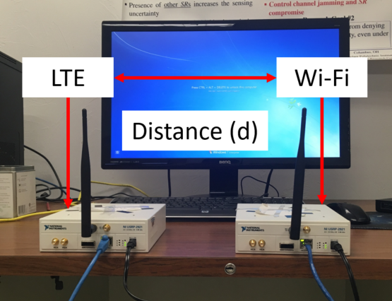
We set up two NI-USRP 2921 devices as a transmitting LTE and an overhearing AP, respectively. The devices were tuned to the 5 GHz U-NII band. The physical layer of the LTE device was programmed to operate according to the LTE standard. The transmission bandwidth was set to 20MHz, whereas the IQ rate was set to 1.92MHz. The LTE frame duration was set to 10ms. Each frame consisted of 10 subframes occupying 2 slots. Each slot had a duration of 0.5ms and allowed for the transmission of 6 OFDM symbols. The duration of each OFDM symbol was set to 83.4s of which s corresponded to the extended CP. The AP sampled the LTE signal on the same band, without implementing any further decoding. The experiment setup is shown in Fig. 13(a).
 |
|||
| (a) | (b) | (c) | (d) |
VI-B Detecting LTE Transmissions
In the first set of experiments, we evaluated the Wi-Fi’s ability in identifying the LTE signals using the CP detection method proposed in Section IV-A. For LTE signals, the number of samples per data symbol was set to and for the CP to . The eNB continuously transmitted 6,000 OFDM symbols, repeating the sequence To further ensure that other signals are not misclassified as LTE, we repeated the experiments but configured the transmitting USRP device to send Wi-Fi OFDM symbols. Each Wi-Fi OFDM symbol had a duration of 4s (3.2s for the data symbol and 0.8s for the CP).
| (a) | (b) | (c) |
The AP sampled the LTE signal and applied Algorithm 1 to compute the correlation as a function of the shift . Figure 13(b) shows sample values of for the duration of ten LTE and Wi-Fi symbols. We observe that when an LTE transmits and the correlation windows and align with the CP and its copy, the correlation peaks to values higher than 0.6. The peaks also denote the start time of OFDM symbols. Using the LTE CP detection parameters on Wi-Fi transmissions yields correlation values of almost zero. This is due to the different OFDM symbol length and CP length in Wi-Fi transmissions.
In Fig. 13(c), we show the detection probability and false alarm probability for the CP-based approach, computed over 6,000 OFDM symbols, as a function of the correlation threshold . The was computed as the fraction of LTE symbols that were correctly classified, whereas was calculated as the fraction of Wi-Fi OFDM symbols that were falsely classified to belong to LTE. Intuitively, a greater threshold would lower the false alarm rate but will decrease the detection probability. We observe that for thresholds in the 0.4-0.6 range, , whereas . Following these experiments, we set the detection threshold to 0.4.
In the next experiment, we investigated the effect of the received signal strength (RSS) on the detection probability. We repeated the LTE signal detection experiment while moving the eNB away from the AP. In Fig. 13(d), we show and as a function of the RSS at the AP. The signal correlation threshold was set to 0.4. Even at low power levels, remains high whereas remains quite low with the exception of -70dBm, which is close to the CCA threshold for detecting any activity.
VI-C Differentiating between eNBs
In this set of experiments, we evaluated the LTE frame attribution algorithm for classifying LTE frames to different eNBs. In the first part of the experiments, one USRP transmitted LTE frames with the same primary and secondary synchronization signal (SSS/PSS) while the second USRP sampled the signal. The signal correlation was calculated over a total of 640 samples per frame, which is equal to the combined length of the two OFDM symbols carrying the SSS and PSS fields.
One practical issue in correlating the sampled PSS and SSS fields over different frames is the fact that the channel changes over time. Whereas the channel attenuation could remain relatively constant for a static LTE-AP distance, the phase of the impulse response could vary more rapidly. Indeed during our experiment, we noted an almost constant phase difference between samples of the same fields that belong to different frames of the same LTE ID. Figure 14(a) shows the absolute phase difference between the samples carrying the PSS and SSS fields in two consecutive frames as a function of the OFDM sample index ,
| (24) |
where and are the phases of the sample in the samples carrying both SSS and PSS fields in the and LTE frames, respectively. We observe a fixed shift when both frames belong to the same LTE ID. This fixed shift is due to the coherence time of the channel. The channel remains relatively constant over the transmission of one frame, but changes over multiple frames. On the other hand, when two frames carry different PSS and SSS fields, the phase difference is random. To improve the eNB identification method, we apply a compensation technique for the channel response phase in Step 4 of the frame attribution algorithm, which operates as follows.
| (a) | (b) | (c) |
- •
The AP extracts samples representing , i.e., the SSS and PSS fields of the LTE frame. Denote the phases of the samples in by vector .
- •
For each signature stored in its database, the AP calculates the mean difference between and the vector denoting the phases of the corresponding samples in ,
(25) - •
The phase part of is compensated by as follows
(26) - •
The AP computes the correlation between and after the former has been phase-compensated, using equation (26).
We emphasize that the proposed phase compensation method does not require decoding LTE transmissions at the AP, as all operations occur on signal samples. Fig. 14(b) shows for 10 LTE frames in the following cases: (1) frames from the same eNB, (2) frames with the same PSS (cell ID) but different SSS (eNB ID), and (3) frames with different PSS and SSS fields. For the first case, we always have a high correlation as all frames belong to the same LTE. For the second and third cases, frames belong to different eNBs, thus the correlation is much lower. In Fig. 14(c), we plot the detection and false alarm probabilities as a function of the detection threshold, we vary the threshold from 0.1 to 0.9. The false alarm represents the case of the same cell ID but different SSS, whereas represents the case of the different PSS and SSS. The value of is almost zero even for very low thresholds. For the second case, becomes almost zero when the detection threshold is selected to be higher than 0.35, whereas remains close to 1. The experiments confirm that applying the correlation technique on the PSS and SSS fields can successfully attribute LTE signals to the transmitting eNB.
| (a) | (b) | (c) |
| (a) | (b) |
VI-D Transmission Round Estimation
In the final set of experiments, we evaluated the transmission round estimation algorithm discussed in Section IV-D. First, we evaluated Step 1 in Algorithm 3 by implementing a collision between LTE and Wi-Fi frames and applying the CP-based correlation method. Figure 15(a) shows the correlation as a function of the OFDM symbol index for a sample LTE collision with Wi-Fi. We observe that once the LTE frame starts, correlation peaks start to appear. Although the correlation is not as high as the case when the samples are interference-free, it is still sufficiently high to indicate the start of the LTE frame.
Furthermore, we implemented retransmissions of the same LTE frame and computed the signal correlation over a window of 38,400 samples, which is the length of one LTE frame. The phase compensation mechanism was also used here to account for the variations in the CIR. The phase difference was computed over the entire frame. Figure 15(b) shows the correlation between 10 pairs of frames when the frames in each pair are identical (retransmission due to channel impairments), identical but one is corrupted by another transmission (collision), and when they differ (not a retransmission). In the collision case, half of the samples representing the initial LTE frame are corrupted. We observe that the signal correlation between two identical transmissions is substantial enough to distinguish it from two different transmissions, even if some of the samples are corrupted.
In Fig. 15(c), we show the probability of detecting a retransmission when both the original frame and the retransmission do not collide with other frames. Moreover, we show the detection probability of a retransmission when the original frame collided with another frame and the false alarm probability as a function of the threshold . The false alarm is evaluated by changing the payload of consecutively transmitted LTE frames. We observe that the correlation technique yields a nearly perfect detection for any threshold less than 0.8 when the frames are not corrupted and 0.2 when the frames are corrupted. The false alarm, on the other hand, is close to zero for any threshold greater than 0.1. Selecting a threshold value equal to 0.2 allows the identification of retransmissions for both clean and corrupted frames. The high accuracy is attributed to the large number of samples used in the computation of the correlation relative to the prior correlation mechanisms that use fewer samples.
VII Performance Evaluation
To validate the proposed misbehavior detection framework, we further implemented an event-based simulation for the LTE/Wi-Fi coexistence. Specifically, we deployed a set of LTE and Wi-Fi devices in the same collision domain so that activity from every device affects the behavior of others. The eNBs followed the LTE-LAA standard whereas the APs implemented the IEEE 802.11ac protocol. LTE protocol parameters were considered perfectly detected using the proposed implicit techniques. To isolate the impact of misbehavior, frame losses occurred only due to collisions (perfect channel conditions). Each experiment was run for 100,000 events, where each event corresponds to a transmission attempt by any device. For each device, we evaluated the transmission attempt rate defined as the number of times a device tried to transmit (backoff reached zero) including collisions, over the total number of attempts by any device. This metric indicates the success rate in seizing the common medium. We further evaluated the detection and false alarm probabilities, and , under different misbehavior scenarios.
| (a) | (b) | (c) |
| (a) | (b) |
| (a) | (b) | (c) | (d) |
VII-A Effect of LTE Misbehavior on Wi-Fi
In the first set of experiments, we evaluated the effect of LTE misbehavior on the Wi-Fi channel access opportunities. LTE misbehavior was implemented by adopting smaller values for the default CW. The LTE chose its backoff uniformly in , where is the modified CW that is chosen independently of the frame class and transmission round. In Fig. 16(a), we show the transmission attempt rate as a function of the normalized reduction in the CW size, denoted by , where is the compliant CW ( indicates no misbehavior). We set , the fraction of time that the LTE remains compliant, to 0.5. We considered the coexistence of one LTE with and Wi-Fi APs, respectively. The Wi-Fi channel access opportunities are shown to degrade when the LTE adopts smaller values whereas the opportunities equalize when approaches . In addition, the LTE maintains its channel access advantage even when a larger number of Wi-Fi stations compete (note that for , the Wi-Fi attempt rate is normalized per AP). The degradation in the Wi-Fi attempt rate goes up to 50%. Figure 16(b) gives similar intuition when the fraction of time that the LTE misbehaves is varied and .
Next, we studied the relation between the number of APs competing with the LTE and the attempt rate. We evaluated the effect of two misbehavior types. In Type 1 misbehavior, the LTE always decreases the CW to , whereas in Type 2 it used the compliant CW (), but disregarded the CW exponential growth after collisions. We compared the attempt rate under the two misbehavior types with the attempt rate when there is no LTE misbehavior, represented by the labels LTE and Wi-Fi with no type. In Fig. 16(c), we show the attempt rate as a function of . An interesting point here is that the effect of Type 1 misbehavior is more prominent at small ’s, whereas Type 2 misbehavior has a higher impact at high . Overall, Type 1 misbehavior has higher impact than Type 2, as it affects all retransmission rounds.
In the previous set of experiments, the LTE and all Wi-Fi APs used the same priority class, i.e., almost similar backoff parameters. In the next set of experiments, we varied the priority class and measured the achieved attempt rate. In Fig. 17(a), the APs employed a lower priority class that utilizes a smaller CW. We observe that the Wi-Fi performance is almost the same as that of the LTE because reducing the CW for the LTE to equalizes the channel access opportunities for all devices. As expected, the LTE gains are significant when the LTE uses a lower class than Wi-Fi and the LTE also misbehaves. These results are shown in Fig. 17(b) where we see a larger difference in performance relative to Fig. 16(c), where the LTE and the APs operate the same class.
VII-B Receiver Operating Characteristic Curves
To investigate the efficacy of our misbehavior detection framework, we studied the tradeoff between and , for different values of the misbehavior detection threshold , through receiver operating characteristic (ROC) curves.
VII-B1 Manipulation of the CW
To measure , we implemented a Type 1 misbehavior strategy with when the LTE misbehaved 50% of the simulation time. To measure , we applied our detection framework when the LTE did not misbehave. Figure 18(a) shows the ROC curve for different lengths of observation set (sizes of set ) denoted by . Indeed, with the increase in the length of the observation set, the ROC approaches the optimal curve indicating that our system can operate with almost sure detection and almost zero false alarm probability. In Fig. 18(b), we see the effect of the fraction of time the LTE misbehaves. Even at low levels of misbehavior (e.g. ), the misbehavior is detectable.
VII-B2 Manipulation of the defer time
We further evaluated the performance of the proposed detection framework when the LTE manipulates the defer time . To simulate this misbehavior, we implemented an LTE that uses the defer time from traffic class (i.e., ) while transmitting frames that belong to class (). Our simulations in Fig. 18(c) show an almost perfect ROC curve for any non-zero false alarm probability, when and . The results are justified by the fact that the consistent selection of a smaller defer time skews the estimated distribution of backoff values in a detectable manner. This is a detectable phenomenon for any that fixes the false alarm probability to a given value.
VII-B3 CCA threshold manipulation
We further performed another set of experiments to evaluate the manipulation of the CCA threshold. A selection of a higher CCA threshold increases the number of APs that are ignored by the LTE. To simulate the CCA threshold manipulation scenario, we uniformly deployed multiple APs and one LTE in a square area of meters. We set the transmission power of each Wi-Fi AP to 20dBm and modeled the channels between terminals using the free path-loss model (the channel model is not really important here). We set the carrier frequency to 5 GHz.
We evaluated the performance of our detector when the CCA threshold is set to -63, -68, and -72dBm (the LTE-LAA standard sets the CCA threshold to -73 dBm). To highlight the effect of CCA threshold manipulation, we implemented a deployment of APs. Here, we increased the number of APs to ensure that we have a non-negligible number of ignored Wi-Fi transmissions. This is shown in Fig. 19(a) where we plot the average number of ignored Wi-Fi transmissions, normalized over the LTE channel access attempts. For instance, when the CCA threshold is set to -72 dBm, the LTE ignores on average one Wi-Fi transmission every ten channel access attempts. On the other hand, the LTE ignores on average one Wi-Fi transmission every other channel access attempt when the threshold is set to -68 dBm. The high number of APs is a relevant scenario in urban areas where there are dense deployments of APs.
In Fig. 19(b), we show the ROC for the three CCA thresholds. We observe that when the CCA is lowered by more than 5dBm, the ROC approaches the optimal one. However, our framework does not detect accurately a small change in the CCA. Such misbehavior creates an imperceptible advantage for the LTE in terms of channel access opportunities as the LTE only ignores, on average, one Wi-Fi transmission each ten channel access attempts as shown in Fig. 19(a).
| (a) | (b) |
VII-C Unsaturated traffic
In the last set of experiments, we studied misbehavior under unsaturated traffic conditions. We implemented a Poisson frame arrival process with an average rate for each device. We measured the saturation level by the percentage of time a device’s queue stays empty and denoted this parameter by . A device is saturated if , i.e., it always has a frame to transmit.
In Fig. 20, we show the effect of the arrival rate on the attempt rate for different levels of saturation. We implemented a Type 1 misbehavior strategy where the eNB transmits class 3 frames but reduces the contention window to The eNB misbehaved half the time . Figure 20(a) shows the saturation levels of both LTE and Wi-Fi with and without LTE misbehavior when the Wi-Fi traffic is always saturated and one eNB competes with five APs. Figure 20(b) shows the respective attempt rates. Here, the arrival rate is normalized by which is the maximum service rate (transmissions per second) that meets the medium capacity. In Fig. 20(a), we note that always equals zero for the Wi-Fi APs, as they are backlogged by design. For the LTE station, we observe that when the LTE misbehaves, saturation occurs at a higher arrival rate indicating that the LTE gains an advantage in accessing the channel sooner.
Figure 20(b) shows that when the arrival rate is low, misbehavior has no effect on the attempt rate of the Wi-Fi. However, when increases and the devices approach saturation, the gap between the attempt rate, with and without misbehavior, increases. As expected, the attempt rate gap remains constant after saturation is reached (and is consistent with the results shown in Fig. 17).
Figures 20(c) and 20(d) show the same experiments, but when the APs remain unsaturated while the arrival rate for the LTE increases. The unsaturated condition for the Wi-Fi is also evident in Fig. 20(c), where the Wi-Fi queue is empty over 70% of the time for any From Fig. 20(c), we further observe that the gain from misbehavior is practically diminished. The LTE saturates almost at the same rate Further, we observe in Fig. 20(d) that the LTE misbehavior increases the LTE attempt rate in an imperceptible manner. This makes misbehavior detection less necessary compared to saturated conditions.
Finally, we evaluated the misdetection probability under unsaturated traffic conditions. In Fig. 21(a), we show as a function of the threshold , for Type 1 misbehavior with and . As expected for (i.e., under saturated conditions as seen in Fig. 20 (a)), we have almost perfect detection. Under unsaturated conditions (), the method of excluding observations that yield idle times larger than expected during a backoff process enables us to have a reasonable with careful selection of . Misdetection becomes very small for , however, for this range, the AP is required to collect a large number of observations to avoid false alarms. Generally, this range of is only required whenever the LTE is found operating under unsaturated traffic conditions. Figure 21(b) shows as a function of the arrival rate at the LTE, for Type 1 misbehavior. As expected, approaches zero as we approach saturation.
VIII Conclusion
We studied the problem of LTE misbehavior under the LTE-LAA protocol for coexistent LTE and Wi-Fi systems. We outlined several misbehavior scenarios and developed a suite of implicit monitoring techniques that enable the Wi-Fi system to estimate the operational parameters of the LTE, without decoding LTE signals. This is a desired property as Wi-Fi devices are not necessarily equipped with LTE receivers. Our methods rely on operations in the signal domain to identify and classify LTE transmissions. We evaluated these techniques using an experimental setup and verified their efficiency in practical scenarios.
We further developed a behavior evaluation framework in which a central hub collects all observations from a distributed set of monitoring APs to build a behavior profile for the eNBs and detect misbehavior. We extended our detection method to work reliably for both unsaturated and saturated traffic. We evaluated the performance of our detector via simulations and showed that LTE misbehavior can cause a significant performance degradation for Wi-Fi devices. However, such misbehavior was detectable by our framework with very high probability while achieving a low false alarm probability. Although our framework focuses on the coexistence between LTE and Wi-Fi systems, our ideas can be extended to other coexistence scenarios.
References
- [1] I. Samy, L. Lazos, Y. Xiao, M. Li, and M. Krunz, “LTE misbehavior detection in Wi-Fi/LTE coexistence under the LAA-LTE standard,” in Proceedings of the 11th ACM Conference on Security & Privacy in Wireless and Mobile Networks, 2018, pp. 87–98.
- [2] FCC, “Second memorandum opinion and order: In the matter of unlicensed operation in the TV broadcast band and additional spectrum for unlicensed devices below 900 MHz in the 3 GHz band,” https://apps.fcc.gov/edocs_public/attachmatch/FCC-08-260A1.pdf, 2010.
- [3] A. B. Flores, R. E. Guerra, E. W. Knightly, P. Ecclesine, and S. Pandey, “IEEE 802.11af: a standard for TV white space spectrum sharing,” IEEE Communications Magazine, vol. 51, no. 10, pp. 92–100, 2013.
- [4] Qualcomm, “Qualcomm whitepaper: Extending LTE advanced to unlicensed spectrum,” https://www.qualcomm.com/media/documents/files/white-paper-extending-lte-advanced-to-unlicensed-spectrum.pdf, 2013.
- [5] 3GPP, “TR 36.889: Feasibility study on licensed-assisted access to unlicensed spectrum,” https://portal.3gpp.org/desktopmodules/Specifications/SpecificationDetails.aspx?specificationId=2579, 2015.
- [6] FCC, “FCC 16-89: Use of spectrum bands above 24 GHz for mobile radio services, et al.” https://apps.fcc.gov/edocs_public/attachmatch/FCC-16-89A1_Rcd.pdf, 2016.
- [7] H. He, H. Shan, A. Huang, L. X. Cai, and T. Q. Quek, “Proportional fairness-based resource allocation for LTE-U coexisting with Wi-Fi,” IEEE Access, vol. 5, pp. 4720–4731, 2016.
- [8] Y. Li, F. Baccelli, J. G. Andrews, T. D. Novlan, and J. C. Zhang, “Modeling and analyzing the coexistence of Wi-Fi and LTE in unlicensed spectrum,” IEEE Transactions on Wireless Communications, vol. 15, no. 9, pp. 6310–6326, 2016.
- [9] Z. Guan and T. Melodia, “CU-LTE: Spectrally-efficient and fair coexistence between LTE and Wi-Fi in unlicensed bands,” in IEEE INFOCOM 2016-The 35th Annual IEEE International Conference on Computer Communications. IEEE, 2016, pp. 1–9.
- [10] S. Sagari, S. Baysting, D. Saha, I. Seskar, W. Trappe, and D. Raychaudhuri, “Coordinated dynamic spectrum management of LTE-U and Wi-Fi networks,” in Proceedings of the Dynamic Spectrum Access Networks Symposium. IEEE, 2015, pp. 209–220.
- [11] A. Mukherjee, J.-F. Cheng, S. Falahati, L. Falconetti, A. Furuskär, B. Godana, H. Koorapaty, D. Larsson, Y. Yang et al., “System architecture and coexistence evaluation of licensed-assisted access LTE with IEEE 802.11,” in Proceedings of the IEEE International Conference on Communication Workshop (ICCW). IEEE, 2015, pp. 2350–2355.
- [12] J. Xiao and J. Zheng, “An adaptive channel access mechanism for LTE-U and WiFi coexistence in an unlicensed spectrum,” in Proceedings of the ICC Conference. IEEE, 2016, pp. 1–6.
- [13] Q. Chen, G. Yu, and Z. Ding, “Optimizing unlicensed spectrum sharing for LTE-U and WiFi network coexistence,” IEEE Journal on Selected Areas in Communications, vol. 34, no. 10, pp. 2562–2574, 2016.
- [14] F. Cai, Y. Gao, L. Cheng, L. Sang, and D. Yang, “Spectrum sharing for LTE and WiFi coexistence using decision tree and game theory,” in Proceedings of the IEEE Wireless Communications and Networking Conference, 2016, pp. 1–6.
- [15] S. Zinno, G. Di Stasi, S. Avallone, and G. Ventre, “On a fair coexistence of LTE and Wi-Fi in the unlicensed spectrum: A survey,” Computer Communications, 2017.
- [16] I. Samy and L. Lazos, “Optimum priority class selection under Wi-Fi/LTE coexistence,” in ICC 2019-2019 IEEE International Conference on Communications (ICC). IEEE, 2019, pp. 1–7.
- [17] X. Han, I. Samy, and L. Lazos, “Energy-efficient LTE/Wi-Fi coexistence,” in ICC 2020-2020 IEEE International Conference on Communications (ICC). IEEE, 2020, pp. 1–7.
- [18] M. Hirzallah and M. Krunz, “Intelligent tracking of network dynamics for cross-technology coexistence over unlicensed bands,” in 2020 International Conference on Computing, Networking and Communications (ICNC). IEEE, 2020, pp. 698–703.
- [19] A. H. Y. Abyaneh, M. Hirzallah, and M. Krunz, “Intelligent-CW: AI-based framework for controlling contention window in WLANs,” in 2019 IEEE International Symposium on Dynamic Spectrum Access Networks (DySPAN). IEEE, 2019, pp. 1–10.
- [20] M. Hirzallah, M. Krunz, and Y. Xiao, “Harmonious cross-technology coexistence with heterogeneous traffic in unlicensed bands: Analysis and approximations,” IEEE Transactions on Cognitive Communications and Networking, vol. 5, no. 3, pp. 690–701, 2019.
- [21] M. Hirzallah, Y. Xiao, and M. Krunz, “Matchmaker: An inter-operator network sharing framework in unlicensed bands,” in 2019 16th Annual IEEE International Conference on Sensing, Communication, and Networking (SECON). IEEE, 2019, pp. 1–9.
- [22] ——, “On modeling and optimizing LTE/Wi-Fi coexistence with prioritized traffic classes,” in 2018 IEEE International Symposium on Dynamic Spectrum Access Networks (DySPAN). IEEE, 2018, pp. 1–10.
- [23] S. Sagari, I. Seskar, and D. Raychaudhuri, “Modeling the coexistence of LTE and WiFi heterogeneous networks in dense deployment scenarios,” in Proceedings of the 2015 IEEE International Conference on Communication Workshop (ICCW). IEEE, 2015, pp. 2301–2306.
- [24] R. Ratasuk, M. A. Uusitalo, N. Mangalvedhe, A. Sorri, S. Iraji, C. Wijting, and A. Ghosh, “License-exempt LTE deployment in heterogeneous network,” in Wireless Communication Systems (ISWCS), 2012 International Symposium on. IEEE, 2012, pp. 246–250.
- [25] 3GPP TS 37.213 version 15.0.0 Release 15, “LTE; physical layer procedures for shared spectrum channel access,” 2018.
- [26] T. Tao, F. Han, and Y. Liu, “Enhanced LBT algorithm for LTE-LAA in unlicensed band,” in Personal, Indoor, and Mobile Radio Communications (PIMRC), 2015 IEEE 26th Annual International Symposium on. IEEE, 2015, pp. 1907–1911.
- [27] J. Jeon, H. Niu, Q. Li, A. Papathanassiou, and G. Wu, “LTE with listen-before-talk in unlicensed spectrum,” in Communication Workshop (ICCW), 2015 IEEE International Conference on. IEEE, 2015, pp. 2320–2324.
- [28] R. Yin, G. Yu, A. Maaref, and G. Y. Li, “LBT-based adaptive channel access for LTE-U systems,” IEEE Transactions on Wireless Communications, vol. 15, no. 10, pp. 6585–6597, 2016.
- [29] J. Tan, S. Xiao, S. Han, Y.-C. Liang, and V. C. Leung, “QoS-aware user association and resource allocation in LAA-LTE/WiFi coexistence systems,” IEEE Transactions on Wireless Communications, vol. 18, no. 4, pp. 2415–2430, 2019.
- [30] J. Dai and C. Shen, “Adaptive resource allocation for LTE/WiFi coexistence in the unlicensed spectrum,” in 2018 International Conference on Computing, Networking and Communications (ICNC). IEEE, 2018, pp. 457–462.
- [31] J. Tan, L. Zhang, Y.-C. Liang, and D. Niyato, “Deep reinforcement learning for the coexistence of LAA-LTE and WiFi systems,” in ICC 2019-2019 IEEE International Conference on Communications (ICC). IEEE, 2019, pp. 1–6.
- [32] X. Ying, R. Poovendran, and S. Roy, “Detecting lte-u duty cycling misbehavior for fair sharing with wi-fi in shared bands,” in 2017 IEEE 28th Annual International Symposium on Personal, Indoor, and Mobile Radio Communications (PIMRC). IEEE, 2017, pp. 1–7.
- [33] P. Kyasanur and N. H. Vaidya, “Selfish MAC layer misbehavior in wireless networks,” IEEE Transactions on Mobile Computing, vol. 4, no. 5, pp. 502–516, 2005.
- [34] A. G. Fragkiadakis, E. Z. Tragos, and I. G. Askoxylakis, “A survey on security threats and detection techniques in cognitive radio networks,” IEEE Communications Surveys & Tutorials, vol. 15, no. 1, pp. 428–445, 2013.
- [35] J. Tang, Y. Cheng, and W. Zhuang, “Real-time misbehavior detection in IEEE 802.11-based wireless networks: An analytical approach,” IEEE Transactions on Mobile Computing, vol. 13, no. 1, pp. 146–158, 2014.
- [36] M. Li, S. Salinas, P. Li, J. Sun, and X. Huang, “MAC-layer selfish misbehavior in ieee 802.11 adhoc networks: Detection and defense,” IEEE Transactions on Mobile Computing, vol. 14, no. 6, pp. 1203–1217, 2015.
- [37] Y. Zhang and L. Lazos, “Vulnerabilities of cognitive radio MAC protocols and countermeasures,” IEEE Network, vol. 27, no. 3, pp. 40–45, 2013.
- [38] B. Chen, J. Chen, Y. Gao, and J. Zhang, “Coexistence of LTE-LAA and Wi-Fi on 5 GHz with corresponding deployment scenarios: A survey,” IEEE Communications Surveys & Tutorials, vol. 19, no. 1, pp. 7–32, 2017.
- [39] M. Hirzallah, W. Afifi, and M. Krunz, “Full-duplex spectrum sensing and fairness mechanisms for Wi-Fi/LTE-U coexistence,” in Global Communications Conference (GLOBECOM), 2016 IEEE. IEEE, 2016, pp. 1–6.
- [40] A. L. Toledo and X. Wang, “Robust detection of selfish misbehavior in wireless networks,” IEEE journal on selected areas in communications, vol. 25, no. 6, 2007.
- [41] Y. Zhang and L. Lazos, “Countering selfish misbehavior in multi-channel MAC protocols,” in INFOCOM, 2013 Proceedings IEEE. IEEE, 2013, pp. 2787–2795.
- [42] S. Gollakota and D. Katabi, Zigzag decoding: combating hidden terminals in wireless networks. ACM, 2008, vol. 38, no. 4.
![[Uncaptioned image]](2104.02776v1/Samy.jpg) |
Islam Samy received the B.S. degree in electrical engineering from Alexandria University in 2011 and the M.Sc. degree in wireless communication from Nile University in 2014. He is currently pursuing the Ph.D. degree with the Electrical and Computer Engineering Department, The University of Arizona, where he is also a Graduate Research Assistant. His main research interests include secure and fair resource allocation for heterogeneous coexisting systems, wireless communication, and information theory. |
![[Uncaptioned image]](2104.02776v1/Xiaoh.png) |
Xiao Han received the BE degree in electrical engineering from Northwest A&F University, Xianyang, China, in 2016, and MS degree in electrical and computer engineering from University of Arizona, Tucson, United States, in 2019. He is currently working toward the PhD degree in computer science at University of South Florida, Tampa, United States. His research interests include wireless networks and network security. |
![[Uncaptioned image]](2104.02776v1/lazos.png) |
Loukas Lazos is a Professor of Electrical and Computer Engineering at the University of Arizona. Dr. Lazos received his Ph.D. degree in Electrical Engineering from the University of Washington in 2006. His research interests are in the areas of network security, privacy, and wireless communications. His current research focuses on secret-free authentication methods for IoT devices, integrity verification of physical properties, secure and fair channel access for emerging wireless technologies, and fair resource allocation for heterogeneous coexisting technologies, and private information retrieval. Dr. Lazos is the recipient of the US National Science Foundation (NSF) Faculty Early CAREER Development Award (2009) for his research in security of multi-channel wireless networks. He has served as a technical program chair for the IEEE CNS conference, the IEEE GLOBECOM symposium on communications and information systems security and the IEEE DSPAN workshop. He is an associate editor for the IEEE Transactions on Information and Forensics Security journal and the IEEE Transactions on Mobile Computing journal. He has also served and continues to serve on the organization and technical program committees of many international conferences and on expert panels of several government agencies. |
![[Uncaptioned image]](2104.02776v1/MingLi.jpg) |
Ming Li is an Associate Professor in the Department of Electrical and Computer Engineering of University of Arizona, and also affiliated with the Computer Science Department. He was an Assistant Professor in the Computer Science Department at Utah State University from 2011 to 2015. He received his Ph.D. in ECE from Worcester Polytechnic Institute, MA, in 2011. His main research interests are wireless and cyber security, with current emphases on cross-layer optimization and machine learning in wireless networks, wireless physical layer security, privacy enhancing technologies, and cyber-physical system security. He received the NSF Early Faculty Development (CAREER) Award in 2014, and the ONR Young Investigator Program (YIP) Award in 2016. He is a senior member of IEEE, and a member of ACM. |
![[Uncaptioned image]](2104.02776v1/YongXiaosmall2.png) |
Yong Xiao(S’09-M’13-SM’15) is a professor in the School of Electronic Information and Communications at the Huazhong University of Science and Technology (HUST), Wuhan, China. He is also the associate group leader in the network intelligence group of IMT-2030 (6G promoting group) and the vice director of 5G Verticals Innovation Laboratory at HUST. His research interests include machine learning, game theory, and their applications in cloud/fog/mobile edge computing, green communication systems, wireless networks, and Internet-of-Things (IoT). |
![[Uncaptioned image]](2104.02776v1/Krunz.jpg) |
Marwan Krunz is the Kenneth VonBehren Endowed Professor in ECE and a professor of computer science at the University of Arizona. He directs the Broadband Wireless Access and Applications Center (BWAC), a multi-university NSF/industry center that focuses on next-generation wireless technologies and applications. He also holds a courtesy appointment as a professor at the University Technology Sydney. He previously served as the site director for the Connection One center. Dr. Krunz’s research emphasis is on resource management, network protocols, and security for wireless systems. He has published more than 300 journal articles and peer-reviewed conference papers, and is an inventor on 12 patents. His latest h-index is 60. He is an IEEE Fellow, an Arizona Engineering Faculty Fellow, and an IEEE Communications Society Distinguished Lecturer (2013-2015). He received the NSF CAREER award. He recently served as the Editor-in-Chief for the IEEE Transactions on Mobile Computing. He also served as editor for numerous IEEE journals. He was TPC chair INFOCOM’04, SECON’05, WoWMoM’06, and Hot Interconnects 9. He was the general vice-chair for WiOpt 2016 and general co-chair for WiSec’12. Dr. Krunz is also an enterpreneur, serving as chief technologist/scientist for two startup companies that focus on 5G and beyond systems and signal intelligence. |