Visual Vibration Tomography: Estimating Interior
Material Properties from Monocular Video
Abstract
An object’s interior material properties, while invisible to the human eye, determine motion observed on its surface. We propose an approach that estimates heterogeneous material properties of an object from a monocular video of its surface vibrations. Specifically, we show how to estimate Young’s modulus and density throughout a 3D object with known geometry. Knowledge of how these values change across the object is useful for simulating its motion and characterizing any defects. Traditional non-destructive testing approaches, which often require expensive instruments, generally estimate only homogenized material properties or simply identify the presence of defects. In contrast, our approach leverages monocular video to (1) identify image-space modes from an object’s sub-pixel motion, and (2) directly infer spatially-varying Young’s modulus and density values from the observed modes. We demonstrate our approach on both simulated and real videos.
![[Uncaptioned image]](2104.02735v4/pipeline.png)
1 Introduction
The subtle motions of objects around us are clues to their physical properties. Among such properties are stiffness and density, which dictate how an object will respond to environmental forces. As humans, we can vaguely characterize how stiff or heavy a material is, such as when we infer that a rubber basketball will bounce higher than a ceramic bowling ball by tapping on its surface. Most engineering applications, however, require a greater level of detail, such as when an aeronautical engineer must faithfully simulate how an airplane wing will react to wind turbulence. In computer vision and graphics, a full characterization of an object’s material properties allows one to faithfully simulate its behavior. These scenarios require non-destructive testing to obtain physical properties of the object without altering it.
We propose visual vibration tomography, a method to estimate material properties of an object directly from vibration signals extracted from monocular video. Much of non-destructive testing (NDT) has focused on measuring vibrations to identify the presence of defects in structures with a known geometry. However, NDT tools are not generally used to determine the precise spatial distribution of physical properties in objects with a heterogeneous interior structure.
We show that we can measure vibrations as sub-pixel motion in 2D video and then use this motion to constrain 3D material-property estimation. Videos have several advantages over existing NDT techniques: while contact sensors and laser vibrometers take point measurements, videos offer spatially dense measurements of surface vibrations. While laser vibrometers are expensive and specialized, cameras are ubiquitous and general-purpose. While existing image-based techniques require stereo cameras for 3D motion tracking, our method shows that in many cases, a monocular view is all you need.
Our motivating insight is that, under fixed geometry, an object’s material properties determine its motion. The inverse direction is also true: motion determines material properties up to a scaling factor. If the motion is small, it can be decomposed into independent modes at natural frequencies, lending itself to a concise mathematical equation linking modes and material properties. This link lays the foundation for our physics-constrained optimization approach. The key challenge of our task is to deal with incomplete and 2D (as opposed to full-field) modes. Despite these challenges, we show that we can estimate material properties from image-space motion and recover full-field modes.
In this paper, we first review related work and the theoretical relationship between modes and material properties. We then show how to extract image-space modes from video and recover material properties (Fig. 1 shows an overview of the method). We demonstrate our approach on simulated data of 3D geometries and discuss the effects of damping and model mismatch. Finally, we present proof-of-concept experiments on real data, showing that we are able to image the shape of unseen material inhomogeneities on drum heads and the presence of a defect in a real 3D Jello cube. These experiments demonstrate promise for the future of the approach in more challenging environments. 11 1 Project website: http://imaging.cms.caltech.edu/vvt
2 Related Work
2.1 Material Analysis from Images and Video
In computer vision, scene understanding is an important goal that includes, among many tasks, characterization of materials. Previous work has estimated material categories liu2010exploring; bell2015material; Schwartz_2013_ICCV_Workshops and surface properties sharan2008image; ho2006direction from images. In contrast to static images, videos have been used to estimate material properties, although these are often restricted to specific object categories, such as fabrics bhat2003estimating; bickel2010design; Wang:2011:DDE; miguel2012data; bouman2013estimating and trees wang2017botanical. Other work has inferred material properties from 3D point clouds wang2015deformation; kim2017data and known external forces xu2015interactive, but such measurements are harder to obtain than a 2D video. “Visual vibrometry” davis2015visual; visvib2017pami uses a video’s motion spectrum to estimate stiffness and damping of fabrics and rods. This is a promising step towards a general approach for estimating material properties, but it is restricted to homogenized properties. In a similar vein, others have used video data to identify structural modes chen2014structural; YANG2020110183; s19051229. Davis et al. demonstrated how to visualize image-space modes and use them for plausible simulation davis2014visual; davis2015image.
2.2 Traditional NDT
Non-destructive testing (NDT) is an umbrella term for any technique that collects data of a material or structure without damaging it. Usually, the goal is to identify defects or material inconsistencies that would change the expected behavior of the object. Laser vibrometry durst1976principles and digital image correlation (DIC) chu1985applications are popular tools for measuring surface displacements. Laser vibrometry has been used to examine the integrity of building structures nassif2005comparison; roozen2015determining and materials emge2012remote; chen2014acoustic. DIC also has been used to identify defects in 2D structures speranzini2014technique; tung2008development; feiteira2017monitoring; wu2011experimental; helm2008digital. Both laser vibrometry macpherson2007multipoint; martarelli2001automated and DIC ha2015modal; trebuvna2014experimental can be used for modal analysis, which involves identifying modal frequencies and shapes of a structure. While usually regarded as a verification tool rather than a means to directly infer material properties, recovered modal information has been used to solve for homogenized material properties davis2015visual; foti2012ambient. However, to our knowledge, modal analysis has not been used to solve the more challenging inverse problem of quantifying the heterogeneous properties addressed in this paper.
3 Background
3.1 Modal Analysis
Every object has resonant, or natural, frequencies. At each resonant frequency, the object vibrates periodically in a particular shape, called a mode. The vibration of a linear elastic object can be decomposed into independent modes.
In the finite element method (FEM), we model an object as a mesh, composed of elements that each take on material-property values. The mechanical properties that determine an object’s vibration are Young’s modulus (), Poisson’s ratio (), and density (). and define the stiffness of connections between vertices, while defines the mass distribution. In this discretized model, the stiffness matrix describes the stiffness between each pair of total DOFs, and the mass matrix describes the mass concentrated between each pair of DOFs. A mode and frequency are an eigenvector-eigenvalue solution of the generalized eigenvalue problem:
| (1) |
As Fig. 2 illustrates, a small change in material properties (within a fixed geometry) results in a small change in modal motion. As most solid materials have Poisson’s ratio POPLAVKO201971, the principal properties affecting motion are Young’s modulus, which determines , and density, which determines . Our method is based on the insight that mode shapes on the surface of an object may reveal internal spatial inhomogeneities in these properties.

3.2 Challenge of Monocular Material Estimation
We begin by setting up a simplified version of the inverse problem. Assuming we perfectly measure all modes and frequencies , then by Eq. 1, we have the following minimization problem:
| (2) |
where is the matrix whose columns are modes , and is the diagonal matrix containing eigenvalues . For a known geometry, this is a convex problem with respect to and . However, Eq. 2 requires that we have access to all 3D modes and frequencies. In contrast, we will be working with experimentally-observed, image-space modes, incurring the following challenges:
- 1.
Unseen degrees of freedom (DOFs). We typically only observe a fraction of an object. For example, when observing a 3D cube with a monocular camera, one can see at most three of its sides, projected onto two directions of motion. Consider an 8x8x8 cubic mesh, which has vertices. With three directions of motion, it has total DOFs. But a single monocular view of three sides of the cube can only observe vertices, moving in two directions of motion, amounting to image-space DOFs. This alone limits us to observing fewer than 20% of the full-field DOFs for an 8x8x8 cube.
- 2.
Unseen modes. Theoretically, for discrete meshes, there are as many modes as there are DOFs. However, we can only capture modes at frequencies below the Nyquist sampling rate of the camera, which is .
- 3.
Noise. Aside from camera noise, there is noise from motion extraction, particularly in non-textured regions.
Due to limited data, the problem of solving for and (Eq. 2) is ill-posed.22 2 For a known geometry and complete mode and eigenvalue information, and are fully determined up to a scaling factor. As Fig. 3 shows, observed data typically accounts for a tiny fraction of the matrices involved.
4 Approach
Our aim is to use motion features from a video to estimate material properties. This involves two stages: (1) motion extraction and image-space mode identification, and (2) solving for material properties that best match the observed image-space modes. The input is a video of an object, of which a mesh is known, and we assume that it is vibrating under linear elasticity (i.e., small motion). The output is two 3D images showing voxelized Young’s modulus and density values throughout the object.
4.1 Extracting Image-Space Modes from Video
Motion extraction: Since our approach relies on small, often imperceptible, motions, we need a way to extract sub-pixel motions from video. To quantify the displacements, we use the phase-based approach of Wadwha et al. wadhwa2013phase, which computes local phase shifts in a complex steerable pyramid simoncelli1995steerable; simoncelli1992shiftable; portilla2000parametric. This method has the advantage over other tracking methods (e.g., optical flow) of being robust to tiny motion, down to 0.001 pixel davis2015visual. The phase shifts are converted to pixel displacements using the approach proposed by Fleet and Jepson fleet1990computation; wadhwa2017motion. To increase the signal-to-noise ratio, we filter out outlier pixels (i.e., top 1% of displacement magnitudes) and then apply an amplitude-weighted Gaussian blur. The result of this step is a motion field for each frame, which quantifies the horizontal and vertical displacement at each pixel relative to the first frame.
Identifying image-space modes: Modes are simply periodic motions occurring at particular frequencies, so we would expect them to appear as peaks in the power spectrum of motion amplitude. As is done in previous work that extracts image-space modes davis2015image; davis2014visual; visvib2017pami, we perform a discrete Fourier transform on the motion fields to analyze them in frequency space. To make this more concrete, let and be the horizontal and vertical displacements, respectively, at each pixel at frame . The 1D FFT across time of these displacement fields results in complex-valued and , corresponding to frequencies Hz for . The motion power at frequency is then defined as (dropping notation for clarity). A peak in the power spectrum ideally corresponds to a natural frequency and image-space mode given by .
Sampling image-space modes at mesh vertices: To approximate the 3D-to-2D projection matrix, a user manually identifies the pixel locations of several “reference” mesh vertices, and is the projection matrix that best maps the corresponding mesh coordinates to the image. Using , we map all of the mesh vertices from their 3D coordinates to 2D image coordinates. We then sample each image-space mode at the pixel locations of visible mesh vertices. For mode , we construct a vector that contains the horizontal and vertical displacements of each mesh vertex at the corresponding natural frequency. Supposing we observe out of mesh vertices, the vector has the form
| (3) |
where is the horizontal (pixel) displacement and the vertical (pixel) displacement of vertex . Unseen vertices are assigned displacements of 0, and for notational clarity, we position them at the end of the vector.
4.2 Estimating Material Properties
The matrices and are functions of Young’s modulus and density. While typically expressed as global matrices, they can be decomposed into local matrices, which scale linearly with local material properties. As a result, and can each be written as a weighted sum of “unit” local matrices. Specifically, we voxelize the volume containing the mesh so that each voxel contains a sub-collection of mesh elements. Given Young’s modulus and density for each voxel, we express the global matrices as
| (4) |
where and are “unit” local stiffness and mass matrices, which we assemble using FEniCS alnaes2015fenics, and is the number of voxels. This allows us to represent and as functions of vectors .
4.2.1 Optimization Formulation
Data-matching objective: Suppose we have modal observations, where and are the -th observed image-space mode and natural frequency, respectively. We would like to determine the voxel-wise Young’s modulus values and density values that, when assembled into global stiffness and mass matrices, result in 3D modes that agree with when projected onto image-space. Since we do not know the full-field 3D modes, we need to include them as decision variables. Intuitively, the data-matching objective is to minimize for each .
Regularization: To make the solution well-defined, we choose to minimize total squared variation (TSV) of and , which encourages spatial smoothness. Moreover, since we are estimating both stiffness and mass, the objective function can become arbitrarily low if we do not constrain the range of material-property values; this is because scaling and by a factor of still satisfies the generalized eigenvalue equation: . To resolve this ambiguity, we choose to minimize the deviation of from a mean value . Regardless of , the relative differences in , will not change, and for defect characterization, we generally only care about relative changes.
The resulting optimization problem is written as
| (5) | ||||
| s.t. | ||||
where , , and are hyperparameters that balance the objective terms. The effects of the regularization weights ( and ) are discussed in the supplementary material.
4.2.2 Optimization Strategy
As defined in Eq. 6, we approximately solve Eq. 5 via a dual formulation of the problem. The eigen-constraints in Eq. 5 are too strict to enforce directly, so we incorporate them as quadratic penalties in the dual problem. The weight of each penalty term is a dual variable, , and we apply dual ascent to gradually increase these penalty weights.
| (6) | ||||
| s.t. |
Eq. 6 is a non-convex problem, but it is quadratic with respect to for fixed , and it is quadratic with respect to for fixed . Our procedure is to iteratively compute the closed-form solution for and then , thereby minimizing the objective function at each step. We update the dual variables according to
| (7) |
where is the dual-variable update rate. Once the decision variables have converged, we output the minimizing solution . and are the voxel-wise estimated Young’s modulus and density values.
5 Simulated Experiments
We test our approach on the simulated vibration of 3D cubes with “defects,” and we discuss the practical concerns of complex geometries, model mismatch, and damping.
5.1 Creating Synthetic Data
Cube model: We model a cube as a 10x10x10 hexahedral mesh, similar to a voxel grid. Each of the 1000 voxels is assigned a Young’s modulus and density that correspond to either the primary material or a defect material. The material properties are chosen to resemble Jello and clay, respectively ( Pa, kg/m3, Pa, kg/m3). We set a homogeneous Poisson’s ratio of POPLAVKO201971.
Vibration animation: Once the cube’s mesh and material properties have been defined, we run a transient analysis in COMSOL comsol, a commercial FEM software. The analysis calculates the cube’s deformation over time given an initial condition. We choose an initial condition that mimics “plucking” a corner of the cube (e.g., an initial displacement vector of cm of the top-front corner) and keep the bottom surface fixed. The resulting simulation represents free vibration with a Dirichlet boundary condition. The simulation is 6 seconds long at 2000 FPS. From the calculated displacements, we create an animation of the cube deforming over time by plotting the motion of random points on the surface of the cube with matplotlib matplotlib.
5.2 Implementation and Evaluation Details
Mode selection: We use scipy’s scipy peak-finder to automatically identify peaks in the log-power spectrum of motion amplitude, as described in Sec. 4.1. For a given simulation, this leads to around 20–30 selected peaks. Most peaks correspond to either a true mode or a linear combination of true modes whose frequencies fall in the same FFT frequency bin. However, a few peaks do not correspond to a true mode; we include these false modes in the synthetic results to best mimic analysis of real videos.
Inference cube mesh: We infer on an 8x8x8 hexahedral mesh. Since the simulations are done with a 10x10x10 mesh, our results indicate robustness to a slight mesh mismatch. In the results presented, the simulation model and inference model use linear elements.
Hyperparameters: For every presented result from simulated data, , , and . Keeping these hyperparameters fixed, we ran a hyperparameter search on a dataset of 12 cubes with various defects to identify good values for (Eq. 6) and (Eq. 7). After testing all combinations of and , we determined to set if the number of input modes is ; otherwise, . The dual variables are always initialized to 1, with . The decision variables and are initialized to homogeneous values of 9000 [Pa] and 1270 [kg/m3], respectively (the true values of the primary material).
Evaluation: Our method recovers relative changes in material properties (see Sec. 4.2.1). As such, the normalized 3D images of estimated Young’s modulus and density should match the true normalized properties. We use normalized correlation between the estimated image and ground-truth image as the reconstruction score. Another way to assess estimated properties is to verify that they produce the same image-space modes and natural frequencies as the true properties (see supplementary material).
5.3 Results
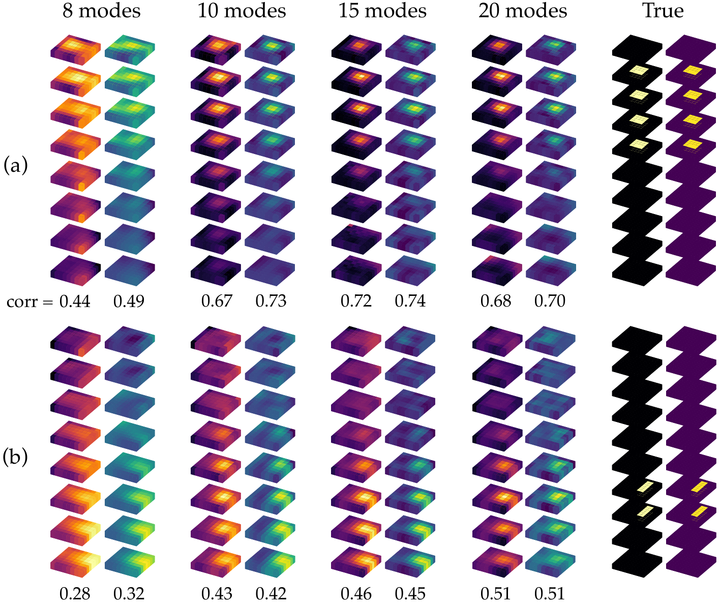
Fig. 4 shows results for two different cubes with defects appearing at different locations. These results are obtained from noisy, motion-extracted image-space modes. As more modes are observed, the inverse problem becomes better constrained, sharpening the image of the interior defect. Also note that a defect near the top of the cube is easier to identify than one near the bottom. This is because the base of the cube is fixed and thus provides less motion signal.
Complex geometry: To demonstrate the approach on a more complex geometry, Fig. 5 shows a volumetric reconstruction of material properties for the Stanford Bunny stanfordbunny. We voxelize the volume containing the tetrahedral mesh33 3 The bunny surface mesh is from https://www.thingiverse.com/thing:151081, and tetrahedralization is done with TetWild tetwild. of the bunny into an 8x8x8 grid and match each mesh element to the nearest voxel, resulting in about 21 elements per voxel. 20 true image-space modes of the monocular view of the bunny shown are used for this reconstruction.

We next consider some challenges that may arise with real-world data: geometric mismatch and damping. More investigations into model mismatch are provided in the supplementary material.
5.3.1 Geometric Mismatch
Fig. 6 shows what happens when the dimensions of the inference mesh do not match the cube’s true dimensions. We gradually increase the length of the inferred cube geometry in the -direction from 1 to 1.4 times the true length. Scaling the length in one direction results in a gradually degrading estimate of the defect size. However, even with 30% geometric error, we are still able to distinguish that there is a defect located in the central region of the cube.
5.3.2 Damping
Real-world objects exhibit various types of damping, which can affect both the frequencies and relative phases of its modes. To simulate damping, we incorporate Rayleigh damping into our synthetic cubes. Our damping parameters were estimated following the procedure outlined by Davis and Bouman et al. davis2015visual, who fit a Lorentzian curve to a peak in the motion power spectrum to estimate the damping ratio. We find that Jello cubes exhibit significant damping: from a real video of one, we estimated critical damping ratios of 0.01749 at 12.5 Hz and 0.01999 at 15.5 Hz.


Through realistic simulations in COMSOL, we find that damping poses the additional challenge of fewer observable modes. We can increase the number of observed modes by extracting modes from multiple simulations with different initial conditions. For example, “plucking” the top-back corner of a cube will cause slightly different modal expression than “plucking” its top-front corner. Fig. 7 shows reconstruction for damped cubes. From two different plucking conditions, we are able to extract between 7–15 modes and use these modes to coarsely reconstruct the defect.
6 Real-World Experiments
To demonstrate the potential of our approach in the real world, we applied it to real videos of drum heads and Jello cubes. With drum heads, we achieve reconstructions that allow one to discern distinct defect shapes, providing a proof-of-concept for defect discovery and characterization using our approach. The damping of 3D Jello cubes poses a challenge for extracting enough image-space modes for high-fidelity defect reconstruction; nonetheless, we are able to identify heterogeneity in the cube. Please refer to the supplementary material for details about the experiment setups, inference models, and hyperparameters.


6.1 Real Drums
We tested our method on a dataset of real drum heads, each altered with a defect beneath the surface. The defects were created from two materials: nail hardening gel (painted beneath the surface) or acrylic plastic circles (glued onto the bottom of the surface). Although all DOFs of the 2D membrane are visible in the video, solving for material properties is still ill-posed because we observe a limited number of projected modes (see Fig. 9).
Results: Fig. 8 shows estimated Young’s moduli and densities for various drum heads, before and after defects were included. For both materials, the defect appears as a bright region in stiffness. Interestingly, gel and acrylic appear differently in their density estimations. For gel defects, there is a bright, filled region in the density map that corresponds to a higher mass from the defect. For acrylic defects, this change only appears on the edges of the defect. This is possibly because the acrylic circles are much stiffer than gel, which bends along with the rubber membrane. These results indicate that our proposed approach could be used to identify not just the presence of a defect, but also its shape.
6.2 Real Cubes
To gain further insight into practical challenges, we conducted an experiment on a real Jello cube with an interior clay defect. This object is more challenging than the drum membrane in two respects: (1) the high damping of Jello, perhaps due to its water content, and (2) the large proportion of unseen DOFs in the cube geometry. The cube had dimensions 4.9 x 4.7 x 4.5 cm, while the rectangular clay defect was of size 2.2 x 2.9 x 1.4 cm. We recorded three videos of the cube under different initial deformation conditions (e.g., in one video, we lifted and then quickly released the top-front corner of the cube). Multiple videos allowed us to identify more unique modes and average duplicate ones.
We created two COMSOL models that would be comparable to the real Jello cube: one simulated cube had a clay defect and the other did not. The Young’s modulus values of the Jello and clay were set so that the natural frequencies would agree with those observed. The Rayleigh damping parameters were estimated following the method mentioned in Sec. 5.3.2. As illustrated in Fig. 10, the COMSOL image-space modes of the simulated cube with a defect appear similar to those captured from the real Jello cube.
Results: Fig. 11 shows the result of our approach applied to real video data of the Jello cube. The reconstruction is obtained using six unique, motion-extracted image-space modes. As expected based on our findings in Figs. 4 and 7, we are able to recover only a large-scale estimation of material properties with six constraining modes. Still, it is very promising to have identified inhomogeneities in a real 3D object with our method. We further compare this real-data reconstruction to reconstructions obtained from simulated data of a homogeneous cube and one with a defect, showing that we achieve a solution that resembles the solution for the simulated defect cube more than it resembles the solution for the simulated homogeneous cube (Fig. 11).
We have shown one example of attaining simulation quality on a real cube. Further work needs to be done to achieve consistent results across a variety of objects. Additional camera views are one plausible, simple solution.
7 Limitations
Our method assumes that materials are isotropic and linear elastic. Linear elasticity is only satisfied if the object’s motion is small. Further, we assume that the geometry is, at least roughly, known ahead of time (see Fig. 6).
For now, we have validated our method with a high-speed camera. We have not yet demonstrated the approach with consumer-grade cameras that bring additional challenges such as image compression and noise. Generally, the hardware required depends on the amplitude and frequencies of the modes. For large structures that vibrate below 100 Hz MEMORY1995705; kolaini2018spacecraft; vibration2015sampaio, a smartphone camera theoretically provides enough temporal frequency. Objects that vibrate more quickly require high-speed cameras. Tricks such as temporal aliasing via a strobe may expand the capabilities of a camera.
The primary challenge with applying this technique to real-world objects is capturing enough image-space modes to recover interior defects with high fidelity. Damping causes a reduction in the number of modes that can be extracted. We demonstrated that for damped Jello cubes, we could still recover some information from only six image-space modes (Sec 6.2). Even so, in many objects, damping will pose a more significant challenge. In the future, acquiring more modal observations could be solved by exciting modes through mechanical vibration tables.
8 Conclusion
We have shown that it is possible to recover spatially-varying material properties of 3D objects from monocular video, even in regions unseen in the image. This can be done by decomposing 2D surface motion into image-space modes, and then solving for the Young’s modulus and density values that agree with the observed modes. We demonstrated our method on synthetic and real-world data of objects ranging from 2D drum heads to a 3D bunny.
Our results highlight that monocular videos are a simple, yet powerful, source of data for understanding the physical properties of objects around us. We believe that videos are a promising domain for further research into non-destructive testing, turning everyday visual sensors into tools for material characterization.
Acknowledgments
The authors would like to thank Michael Rubinstein and Bill Freeman for their helpful discussions. This work is funded by BP. B.T.F. is supported by an NSF GRFP Fellowship and a Kortschak Scholarship. C.D. and A.C.O. acknowledge support from DOE award no. DE-SC0021358 and NSF award no. 1835735.
References
- (1) COMSOL AB. Comsol multiphysics® v5.5.
- (2) Martin Alnæs, Jan Blechta, Johan Hake, August Johansson, Benjamin Kehlet, Anders Logg, Chris Richardson, Johannes Ring, Marie E Rognes, and Garth N Wells. The fenics project version 1.5. Archive of Numerical Software, 3(100):9–23, 2015.
- (3) Sean Bell, Paul Upchurch, Noah Snavely, and Kavita Bala. Material recognition in the wild with the materials in context database. In Proceedings of the IEEE Conference on Computer Vision and Pattern Recognition, pages 3479–3487, 2015.
- (4) Kiran S. Bhat, Christopher D. Twigg, Jessica K. Hodgins, Pradeep K. Khosla, Zoran Popović, and Steven M. Seitz. Estimating cloth simulation parameters from video. In Proceedings of the 2003 ACM SIGGRAPH/Eurographics Symposium on Computer Animation, SCA ’03, page 37–51, Goslar, DEU, 2003. Eurographics Association.
- (5) Bernd Bickel, Moritz Bächer, Miguel A Otaduy, Hyunho Richard Lee, Hanspeter Pfister, Markus Gross, and Wojciech Matusik. Design and fabrication of materials with desired deformation behavior. ACM Transactions on Graphics (TOG), 29(4):1–10, 2010.
- (6) Katherine L Bouman, Bei Xiao, Peter Battaglia, and William T Freeman. Estimating the material properties of fabric from video. In Proceedings of the IEEE International Conference on Computer Vision, pages 1984–1991, Sydney, Australia, 2013. IEEE.
- (7) Justin G Chen, Robert W Haupt, and Oral Buyukozturk. The acoustic-laser vibrometry technique for the noncontact detection of discontinuities in fiber reinforced polymer-retrofitted concrete. Materials evaluation, 72(10):1305–1313, 2014.
- (8) Justin G Chen, Neal Wadhwa, Young-Jin Cha, Frédo Durand, William T Freeman, and Oral Buyukozturk. Structural modal identification through high speed camera video: Motion magnification. In Topics in Modal Analysis I, Volume 7, pages 191–197. Springer, Berlin, Germany, 2014.
- (9) TC Chu, WF Ranson, and Michael A Sutton. Applications of digital-image-correlation techniques to experimental mechanics. Experimental mechanics, 25(3):232–244, 1985.
- (10) Abe Davis, Katherine L. Bouman, Justin G. Chen, Michael Rubinstein, Oral Büyüköztürk, Frédo Durand, and William T. Freeman. Visual vibrometry: Estimating material properties from small motions in video. IEEE Trans. Pattern Anal. Mach. Intell., 39(4):732–745, 2017.
- (11) Abe Davis, Katherine L Bouman, Justin G Chen, Michael Rubinstein, Fredo Durand, and William T Freeman. Visual vibrometry: Estimating material properties from small motion in video. In Proceedings of the IEEE Conference on Computer Vision and Pattern Recognition, pages 5335–5343, Boston, MA, USA, 2015. IEEE.
- (12) Abe Davis, Justin G Chen, and Frédo Durand. Image-space modal bases for plausible manipulation of objects in video. ACM Transactions on Graphics (TOG), 34(6):1–7, 2015.
- (13) Abe Davis, Michael Rubinstein, Neal Wadhwa, Gautham Mysore, Fredo Durand, and William T. Freeman. The visual microphone: Passive recovery of sound from video. ACM Transactions on Graphics (Proc. SIGGRAPH), 33(4):79:1–79:10, 2014.
- (14) Franz Durst, Adrian Melling, and James H Whitelaw. Principles and practice of laser-doppler anemometry. NASA STI/Recon Technical Report A, 76:47019, 1976.
- (15) Timothy Emge and Oral Buyukozturk. Remote nondestructive testing of composite-steel interface by acoustic laser vibrometry. Materials evaluation, 70(12):1401–1410, 2012.
- (16) João Feiteira, Eleni Tsangouri, Elke Gruyaert, Christine Lors, Ghislain Louis, and Nele De Belie. Monitoring crack movement in polymer-based self-healing concrete through digital image correlation, acoustic emission analysis and sem in-situ loading. Materials & Design, 115:238–246, 2017.
- (17) David J Fleet and Allan D Jepson. Computation of component image velocity from local phase information. International journal of computer vision, 5(1):77–104, 1990.
- (18) Dora Foti, Mariella Diaferio, Nicola Ivan Giannoccaro, and Michele Mongelli. Ambient vibration testing, dynamic identification and model updating of a historic tower. NDT & e International, 47:88–95, 2012.
- (19) NS Ha, HM Vang, and NS Goo. Modal analysis using digital image correlation technique: an application to artificial wing mimicking beetle’s hind wing. Experimental Mechanics, 55(5):989–998, 2015.
- (20) Yunus Emre Harmanci, Utku Gülan, Markus Holzner, and Eleni Chatzi. A novel approach for 3d-structural identification through video recording: Magnified tracking. Sensors, 19(5):1229, 2019.
- (21) Jeffrey D Helm. Digital image correlation for specimens with multiple growing cracks. Experimental mechanics, 48(6):753–762, 2008.
- (22) Yun-Xian Ho, Michael S Landy, and Laurence T Maloney. How direction of illumination affects visually perceived surface roughness. Journal of vision, 6(5):8–8, 2006.
- (23) Yixin Hu, Qingnan Zhou, Xifeng Gao, Alec Jacobson, Denis Zorin, and Daniele Panozzo. Tetrahedral meshing in the wild. ACM Trans. Graph., 37(4):60:1–60:14, July 2018.
- (24) J. D. Hunter. Matplotlib: A 2d graphics environment. Computing In Science & Engineering, 9(3):90–95, 2007.
- (25) Meekyoung Kim, Gerard Pons-Moll, Sergi Pujades, Seungbae Bang, Jinwook Kim, Michael J Black, and Sung-Hee Lee. Data-driven physics for human soft tissue animation. ACM Transactions on Graphics (TOG), 36(4):1–12, 2017.
- (26) Ce Liu, Lavanya Sharan, Edward H Adelson, and Ruth Rosenholtz. Exploring features in a bayesian framework for material recognition. In 2010 IEEE Computer Society Conference on Computer Vision and Pattern Recognition, pages 239–246, San Francisco, CA, USA, 2010. IEEE, IEEE.
- (27) William N MacPherson, Mark Reeves, David P Towers, Andrew J Moore, Julian DC Jones, Martin Dale, and Craig Edwards. Multipoint laser vibrometer for modal analysis. Applied optics, 46(16):3126–3132, 2007.
- (28) M Martarelli, GM Revel, and C Santolini. Automated modal analysis by scanning laser vibrometry: problems and uncertainties associated with the scanning system calibration. Mechanical systems and signal processing, 15(3):581–601, 2001.
- (29) Eder Miguel, Derek Bradley, Bernhard Thomaszewski, Bernd Bickel, Wojciech Matusik, Miguel A Otaduy, and Steve Marschner. Data-driven estimation of cloth simulation models. In Computer Graphics Forum, volume 31, pages 519–528, Hoboken, NJ, USA, 2012. Wiley Online Library, Wiley Online Library.
- (30) Hani H Nassif, Mayrai Gindy, and Joe Davis. Comparison of laser doppler vibrometer with contact sensors for monitoring bridge deflection and vibration. Ndt & E International, 38(3):213–218, 2005.
- (31) Yuriy M. Poplavko. Chapter 2 - mechanical properties of solids. In Yuriy M. Poplavko, editor, Electronic Materials, pages 71 – 93. Elsevier, Amsterdam, The Netherlands, 2019.
- (32) Javier Portilla and Eero P Simoncelli. A parametric texture model based on joint statistics of complex wavelet coefficients. International journal of computer vision, 40(1):49–70, 2000.
- (33) Nicolaas Bernardus Roozen, Ludovic Labelle, Monika Rychtáriková, and Christ Glorieux. Determining radiated sound power of building structures by means of laser doppler vibrometry. Journal of Sound and Vibration, 346:81–99, 2015.
- (34) Gabriel Schwartz and Ko Nishino. Visual material traits: Recognizing per-pixel material context. In Proceedings of the IEEE International Conference on Computer Vision (ICCV) Workshops, June 2013.
- (35) Lavanya Sharan, Yuanzhen Li, Isamu Motoyoshi, Shin’ya Nishida, and Edward H Adelson. Image statistics for surface reflectance perception. JOSA A, 25(4):846–865, 2008.
- (36) Eero P Simoncelli and William T Freeman. The steerable pyramid: A flexible architecture for multi-scale derivative computation. In Proceedings., International Conference on Image Processing, volume 3, pages 444–447, Washington, D.C., USA, 1995. IEEE, IEEE.
- (37) Eero P Simoncelli, William T Freeman, Edward H Adelson, and David J Heeger. Shiftable multiscale transforms. IEEE transactions on Information Theory, 38(2):587–607, 1992.
- (38) Emanuela Speranzini and Stefano Agnetti. The technique of digital image correlation to identify defects in glass structures. Structural Control and Health Monitoring, 21(6):1015–1029, 2014.
- (39) F Trebuňa and M Hagara. Experimental modal analysis performed by high-speed digital image correlation system. Measurement, 50:78–85, 2014.
- (40) Shih-Heng Tung, Ming-Hsiang Shih, and Wen-Pei Sung. Development of digital image correlation method to analyse crack variations of masonry wall. Sadhana, 33(6):767–779, 2008.
- (41) Greg Turk and Marc Levoy. Zippered polygon meshes from range images. In Proceedings of the 21st Annual Conference on Computer Graphics and Interactive Techniques, SIGGRAPH ’94, page 311–318, New York, NY, USA, 1994. Association for Computing Machinery.
- (42) Pauli Virtanen, Ralf Gommers, Travis E. Oliphant, Matt Haberland, Tyler Reddy, David Cournapeau, Evgeni Burovski, Pearu Peterson, Warren Weckesser, Jonathan Bright, Stéfan J. van der Walt, Matthew Brett, Joshua Wilson, K. Jarrod Millman, Nikolay Mayorov, Andrew R. J. Nelson, Eric Jones, Robert Kern, Eric Larson, C J Carey, İlhan Polat, Yu Feng, Eric W. Moore, Jake VanderPlas, Denis Laxalde, Josef Perktold, Robert Cimrman, Ian Henriksen, E. A. Quintero, Charles R. Harris, Anne M. Archibald, Antônio H. Ribeiro, Fabian Pedregosa, Paul van Mulbregt, and SciPy 1.0 Contributors. SciPy 1.0: Fundamental Algorithms for Scientific Computing in Python. Nature Methods, 17:261–272, 2020.
- (43) Neal Wadhwa, Justin G Chen, Jonathan B Sellon, Donglai Wei, Michael Rubinstein, Roozbeh Ghaffari, Dennis M Freeman, Oral Büyüköztürk, Pai Wang, Sijie Sun, et al. Motion microscopy for visualizing and quantifying small motions. Proceedings of the National Academy of Sciences, 114(44):11639–11644, 2017.
- (44) Neal Wadhwa, Michael Rubinstein, Frédo Durand, and William T Freeman. Phase-based video motion processing. ACM Transactions on Graphics (TOG), 32(4):1–10, 2013.
- (45) Bin Wang, Longhua Wu, KangKang Yin, Uri M Ascher, Libin Liu, and Hui Huang. Deformation capture and modeling of soft objects. ACM Trans. Graph., 34(4):94–1, 2015.
- (46) Bohan Wang, Yili Zhao, and Jernej Barbič. Botanical materials based on biomechanics. ACM Transactions on Graphics (TOG), 36(4):1–13, 2017.
- (47) Huamin Wang, Ravi Ramamoorthi, and James F. O’Brien. Data-driven elastic models for cloth: Modeling and measurement. ACM Transactions on Graphics, 30(4):71:1–11, July 2011. Proceedings of ACM SIGGRAPH 2011, Vancouver, BC Canada.
- (48) ZhiMin Wu, Hua Rong, JianJun Zheng, Feng Xu, and Wei Dong. An experimental investigation on the fpz properties in concrete using digital image correlation technique. Engineering Fracture Mechanics, 78(17):2978–2990, 2011.
- (49) Hongyi Xu, Yijing Li, Yong Chen, and Jernej Barbič. Interactive material design using model reduction. ACM Transactions on Graphics (TOG), 34(2):1–14, 2015.
- (50) Yongchao Yang, Charles Dorn, Charles Farrar, and David Mascareñas. Blind, simultaneous identification of full-field vibration modes and large rigid-body motion of output-only structures from digital video measurements. Engineering Structures, 207:110183, 2020.