Online change-point detection for a transient change
Abstract
We consider a popular online change-point problem of detecting a transient change in distributions of i.i.d. random variables. For this change-point problem, several change-point procedures are formulated and some advanced results for a particular procedure are surveyed. Some new approximations for the average run length to false alarm are offered and the power of these procedures for detecting a transient change in mean of a sequence of normal random variables is compared.
Keywords:
Boundary crossing probabilities,keywords
[class=AMS]keywords
1 Introduction
The subject of change-point detection (or statistical quality control) is devoted to monitoring and detecting changes in the structure of a time series. This paper considers a popular online change-point problem of detecting a change in distribution of a sequence of i.i.d. random variables. Online change-point problems are concerned with monitoring the structure of a random process(es) whose observations arrive sequentially. For these problems, any good monitoring procedure should reliably alert the user to unexpected changes as soon as possible or with highest probability, subject to a tolerance on false alarms.
Let be a sequence of independent random variables arriving sequentially. The purpose of this paper is to discuss tests for the hypothesis that are identically distributed with some probability density function (pdf) against the alternative that at some unknown change point , the random variables and are identically distributed with density and are identically distributed with pdf such that . Here, is length of the change-point period (signal) and can be known or unknown. Under a standard hypothesis testing framework, the null hypothesis is and hence the pdf is the density of for all . The alternative hypothesis is : and therefore
with . Under , the arrival time of the signal is (it is unknown). Most classical results assume and are known completely; by this, we mean no nuisance parameters are present in the distributions. In later sections, we will briefly discuss tests designed to approach the change-point problem in the presence of nuisance parameters.
A thorough introduction to the field of online (quickest) change-point detection mainly for the case of can be found in, for example, [1, 2, 3, 4]. Some of the most popular online change-point algorithms used in practice are Shewhart’s -chart [5], the CUSUM algorithm [6], the Shiryaev-Roberts procedure [7, 8] and the Exponentially Weighted Moving Average (EWMA) chart [9]. The case of , and hence when a change in distribution occurs it does so permanently, is by far the most popular scenario considered in the change-point literature; a number of influential papers are [10, 11, 12, 13, 14, 15]. The CUSUM and Shiryaev Roberts procedures benefit with their simplicity and proven optimality under suitable optimality criteria; these two procedures will be the focus of discussion for the case . The case of finite , and hence when a change occurs it does so temporarily, has seen considerable attention in the past, see [16, 17, 18, 19, 20, 21, 22, 23]. More recently it has been the focus of attention in the papers of [24, 25, 26]. Examples of areas where detecting a transient change in distributions is extremely important can be found in radar and sonar [27, 28, 29], nondestructive testing [30], and medicine [31]. Non-parametric online change-point detection methods have also become very popular [32, 33]. For the state of the art techniques for multiple change-point detection, see [34, 35, 36, 37]. For sequential change-point detection in high-dimensional time series, a likelihood ratio approach can be found in [38, 39].
This survey is organised as follows. In Section 2, we survey results for and discuss known optimality results for the CUSUM and Shiryaev-Roberts procedures. This section contains well known classical results but is included to introduce the reader to change-point concepts that will be used when considering the transient change-point problem. In Section 3, we assume and discuss a number of online tests for transient changes; the likelihood ratio test providing the inspiration behind all tests. In this Section, we compare procedures when applied for detecting a temporary change in mean of a sequence of Gaussian random variables. We also apply tests for monitoring stability of components used in the Oil and Gas industry.
Throughout this survey we shall use the notation and to denote probability and expectation under . Under the alternative , we shall use the notation and to denote probability and expectation assuming the change-point occurs at .
2 Permanent change in distributions
In this section, we assume ; if a change occurs, it does so permanently. Suppose have been sampled. The likelihood ratio for testing against is
assuming , otherwise .
2.1 The CUSUM and Shiryaev-Roberts procedures
By maximising the statistic over all possible locations of , we obtain the CUSUM statistic
| (2.1) |
The CUSUM stopping rule (when to alert the user to a potential change-point) is
| (2.2) |
An appealing property of statistic (2.1) is the recursive property
The threshold in is chosen on the users tolerance to false alarm risk. Page [6] and Lorden [10] measured false alarm risk through the Average Run Length to false alarm (ARL). This corresponds to choosing such that , where is a pre-defined value chosen by the user but is typically large. How to compute will be discussed later in this section.
The famous CUSUM chart of Page [6] introduces a reflective barrier at zero:
| (2.3) | |||||
The statistics (2.3) and are equivalent on the positive half plane and hence the rule
| (2.4) |
and are equivalent for . The stopping rule is more general than as thresholds are permissable. An approximation for for general distributions and was derived in [40]. Let and (to compute we assume the change-point occurs at time zero). Then
| (2.5) |
Here the constant is called the limiting exponential overshoot. Let be a random walk. Then it can be shown, see [41, Ch. VIII], that
The approximation (2.5) seems extremely accurate. For example, suppose pre-change observations are i.i.d random variables and post-change observations are i.i.d for some known . We have
| (2.6) | |||||
For , Monte Carlo simulations provide . Application of the approximation in (2.5) provides 498. The draw back of the approximation in (2.5) is that requires expensive numerical evaluation.
To construct the Shiryaev-Roberts (SR) procedure, define the generalised Bayesian detection statistic as:
| (2.7) |
Then the SR test is:
| (2.8) |
where is the solution of for some pre-determined . The SR statistic (2.7) satisfies the following recurrence:
2.2 Evaluating ARL for CUSUM and SR tests
Explicit expressions for and are not known. However, they can be numerically obtained by numerically solving particular Fredholm integral equations as proved in [42]. Here it was shown that and can be computed by a unified approach for general Markov statistics. Set . For a sufficiently smooth positive valued function and , let
be a Markov detection statistic with stopping rule
Let be the ARL (note the dependence on ) and set . Then is the solution of the following Fredholm integral equation:
| (2.9) |
For the CUSUM and SR procedures we have and , respectively. To solve this integral equation, we refer to [42].
Approximations for ARL of the CUSUM and SR procedures have been specifically developed for the problem of detecting the change in mean of normal random variables. Here we operate under (2.6). To approximate ARL for both the CUSUM and SR procedures or to narrow the domain of search and more efficiently numerically solve the Fredholm equation (2.9), one could use the following simple approximations developed in [43] and [44] respectively:
| (2.10) | |||||
| (2.11) |
where
The approximations in (2.10) and (2.11) are extremely accurate. In Table 1, one can observe the high accuracy of approximation (2.10) for different thresholds . In fact, (2.11) is remarkably accurate and frequently leads to exact values of ARL. The only slight inconvenience of both approximations is the numerical evaluation required to compute . This quantity can be approximated with , where the constant is defined later in (3.2.1) but can be approximated to three decimal places by . Using this approximation for in (2.10) and (2.11) still results in excellent approximations.
2.3 Optimality criteria
Denote by the set of all stopping times of change-point procedures with ARL of at least . More precisely, where is a stopping time for a sequential change-point procedure. A common criterion for comparing change-point procedures when is the supremum Average Delay to Detection (ADD) introduced by Pollak [12]. Define . Then
| (2.12) |
An optimal change-point procedure would satisfy for all . Finding an optimal procedure for this criterion is very difficult, where in general only asymptotic optimality as (low false alarm rate) is known [12]. Another popular criterion is the worst-case minimax scenario of Lorden [10] defined as
This criterion evaluates the average detection delay conditioned on the worst possible data before the change and then considers the worst possible deterministic change-point. Asymptotic optimality (as ) of the CUSUM chart of Page was proved in [10]. It was subsequently proved in [11] that the CUSUM chart of Page is in fact optimal under this criterion for every .
The SR procedure is optimal for every under the Stationary Average Delay to Detection (STADD) criterion. The STADD criterion praises detection procedures that detect the change as quickly as possible, at the expense of raising many false alarms (using a repeated application of the same stopping rule). Formally, the STADD criterion is defined as follows. Let be a sequence of independent copies of the stopping time . Let be the time the alarm is raised. Let ; this is the index of the first alarm which is not false after false alarms. Then
The STADD criterion is equivalent to the Relative Integral Average Detection Delay (RIADD) measure, see [42], which is defined as:
Both the SR procedure and CUSUM procedure are asymptotically optimal as for the Lorden and the STADD criteria. It is discussed in [42] for both CUSUM and the Shiryaev–Roberts procedure Lorden’s essential supremum measure (2.3) and Pollak’s supremum measure defined in (2.12) are attained at , that is:
Similarly to the computation of and , to obtain and one can numerically solve a Fredholm equation. Instead of setting , let . Also set . Then from [42], is the solution of the Fredholm integral equation given in (2.9). The computation of STADD requires solving a slightly more difficult integral equation and we refer the interested reader to [42] for more discussions.
For the Gaussian example considered in (2.6), the findings of [42] indicate that for small values of say , the CUSUM noticeably outperforms the SR procedure under Lordens criterion. Vice versa, the SR procedure noticeably outperforms CUSUM under the STADD framework. When the change in becomes large, say , the benefits a procedure has over the other diminishes.
3 Transient change in distributions
In this section, we assume and therefore study procedures aimed at detecting a transient change in distributions. Suppose have been sampled. The log likelihood ratio for testing against is
| (3.1) |
3.1 A collection of procedures
For unknown, the log likelihood ratio statistic is obtained by maximising (3.1) over all possible change point locations and transient change lengths:
| (3.2) |
with the stopping rule
| (3.3) |
If there are no nuisance parameters present in and that require estimation, the statistic (3.2) satisfies the recursive property:
| (3.4) | |||||
For large , the statistic (3.2) is very expensive to compute despite the recursive property given in (3.4). For offline change-point problems, this large computational expense may be an inconvenience but it is not a fundamental problem as time is often not an issue. However, for online procedures that require calculations in real time, the statistic is not practical. The assumption that no knowledge of the transient change length is known is unlikely. One can imagine that some prior knowledge about the length of transient change is likely, for example it may be bounded . From here on, this assumption will be made. The log likelihood ratio statistic is:
| (3.5) |
with the stopping rule
If no nuisance parameters require estimation, the statistic satisfies the following recursive property:
This is much easier to compute than (3.2) for large. This recursive property means the stopping rule of can be expressed as:
| (3.6) | |||||
and
Therefore .
If we make the additional assumption that is known exactly and is completely contained within the sample of size , i.e. , then the MOSUM statistic can be obtained by setting in (3.5). For this reason, the statistic can be called the generalised MOSUM procedure. This corresponds to maximising (3.1) over all valid change-point locations :
| (3.7) |
with the stopping rule
In what follows, we will define the MOSUM test for a general window length , with a fixed positive integer. Results for the likelihood ratio test can be obtained by setting . Define the moving sums
Then the stopping rule for a given window length can be expressed as
| (3.8) | |||||
and therefore . The moving sum is the reason behind the MOSUM name.
For the transient change-point problem, the false alarm risk can be measured through ARL. However, this is not the only approach taken in the change-point literature. In [17] and [45] , the false alarm risk is measured through:
| (3.9) |
where is a stopping rule, is your false alarm tolerance (type 1 error) and but as ; recall . Another alternative to the usual ARL constraint has been proposed in [43, 46]. Here, the suggested criterion is
3.2 Detecting a transient change in Gaussian random variables
Consider the problem of detecting the change in mean of normal random variables. Suppose pre-change observations are i.i.d random variables and post-change observations are i.i.d for some . The values of and may be known or unknown, with and playing the roles of nuisance parameters if unknown. We have
| (3.10) | |||||
The offline version of this change-point problem is devoted to testing for change-points in a sample of fixed length and has seen significant attention in the past, see [47, 48, 49, 50, 51]. An excellent survey of several statistics aimed at addressing the offline problem can be found in [52]. Despite the fact defined in (3.5) is a generalisation of given in (3.7), we will initially discuss recent results for . These results will provide inspiration for addressing the much more complicated problems associated with .
3.2.1 The MOSUM statistic
For the MOSUM test, knowledge of is not required to set the ARL constraint; this is because the MOSUM stopping rule given in (3.8) specialised for this Gaussian example is tantamount to:
| (3.11) | |||||
The problem of approximating assuming is known was considered in [25]. Here will recall the main steps in the construction. Define
and consider the standardised versions of :
Then the stopping time is equivalent to the stopping time
| (3.12) |
and hence .
For any integer , the discrete time process is approximated by a continuous time analogue on . The process is a zero mean, stationary Gaussian process with correlation function . The ARL then has the continuous-time approximation
| (3.13) |
where .
Explicit formulas for the probability with were first derived in [53]. Here it was shown
For this reduces to
| (3.14) |
For , formulae for were first derived in [54]; these expressions take different forms depending on whether or not is integer. The result of [54, p.949] states than if is a positive integer then
| (3.15) |
where . For non-integer , the exact formula for is even more complex (the integral has the dimension ) see [54, p.950]. For , (3.2.1) yields
| (3.16) | |||||
The complicated nature of these expressions for made them impractical for the use in the ARL approximation (3.13). One simple yet still very accurate approximation has the form (see [55]):
| (3.17) |
where and the probabilities and are given in (3.14) and (3.16) respectively. Here, and are the standard normal density and distribution functions respectively. The approximation given in (3.17) applied to (3.13) results in the following continuous-time ARL approximation:
This approximation was then corrected in [25, Section 7] for discrete time to improve results for small . This amounted to correcting the probabilities and for discrete time; this was performed by specialising results of D. Siegmund; primarily on expected overshoot a discrete time normal random walk has over a threshold. From [41, p. 225], this expected overshoot was computed as
Define the probability
| (3.19) |
From [25, p. 18]:
where, for with , the probabilities and can be approximated by:
| (3.22) | |||||
Only a one-dimensional integral has to be numerically evaluated for approximating . Tables 2 and Tables 3 demonstrate that (3.2.1) using (3.2.1) and (3.22) is extremely accurate.
| 2 | 2.25 | 2.5 | 2.75 | 3 | 3.25 | 3.5 | |
|---|---|---|---|---|---|---|---|
| (3.2.1) | 126 | 217 | 395 | 759 | 1551 | 3375 | 7837 |
| 127 | 218 | 396 | 757 | 1550 | 3344 | 7721 |
| 2 | 2.25 | 2.5 | 2.75 | 3 | 3.25 | 3.5 | |
|---|---|---|---|---|---|---|---|
| (3.2.1) | 471 | 791 | 1392 | 2587 | 5099 | 10695 | 23918 |
| 472 | 792 | 1397 | 2588 | 5085 | 10749 | 24131 |
3.2.2 The stopping rule
Here, we assume is not known exactly but can be bounded between and . We will initially assume and are known. The stopping rule given in (3.6) specialised for this Gaussian example is tantamount to:
| (3.24) | |||||
and
The short memory of the MOSUM statistic is paramount to the form of the approximation given in (3.23). This short memory is also present for the generalised moving sum statistic and suggests the form of approximations (3.2.1) and (3.23) would also be suitable when applied to . Introduce the probability:
Then the following approximations should also provide high accuracy:
| (3.25) | |||
| (3.26) |
Unfortunately, the probability is complex and to the authors knowledge no formula or approximations are known. The probabilities and can be approximated via simulations; this is not too cumbersome as at most random variables need to be simulated at each iteration. As commonly with large, say , the right tail of the distribution of the random variable is of the most interest. Large deviation theory, see [48, 49], could be used to approximate the right tail of this distribution, however numerical results indicate approximations of these kind would not be accurate enough for general and (those that are not astronomically large). If the prior knowledge that is known, and an explicit formula to approximate or is desired, the following simple heuristic argument could be used. The continuous time analogue of the probability is:
where , , is standard Brownian motion. Ideally, a large deviation approximation for () should be computed. However, for , and large, say , simulation studies indicate that the additional maximisation constraint in () of has very little influence on this probability. If this constraint is ignored, the following large deviation result of [49] can be applied.
Lemma 1.
Suppose , and such that is some fixed number in . Then
To subsequently correct this result for discrete time, it is recommended in [49] to increase the barrier by by , where is defined in (3.2.1). This results in the approximations
| (3.29) | |||||
| (3.30) | |||||
As a result, using the approximations given in (3.25) and (3.26):
| (3.31) | |||||
with
Also
The accuracy of the approximation in (3.25) is demonstrated in Figures 1-2 for different and as a function of . In this approximation, and have been approximated using Monte Carlo simulations with 100,000 repetitions. In these figures, the probability is depicted with a thick dashed black line and is obtained from simulations. The approximation in (3.25) is depicted with a solid blue line. From these figures the high accuracy of approximation (3.25) is clearly demonstrated. In Figures 3-6, we asses the accuracy of the approximation in (3.31). In these figures, for and various , the probability is depicted with a thick dashed black line whereas the approximation provided in (3.31) is shown with a solid red line. The number present on the figure is used to show the value of used. From these figures, we see for large the approximation in (3.31) is adequate. In Tables 4-5 the accuracy of the approximations provided in (3.26) and () are assessed for different . We see the approximation in (3.26) is extremely accurate for all For large , the approximation in () is fairly accurate and has the benefit of explicit evaluation. For small and small , the accuracy of () should deteriorate.


| -5 | -4.5 | -4 | -3.5 | -3 | -2.5 | -2 | |
|---|---|---|---|---|---|---|---|
| (3.26) | 78 | 96 | 116 | 144 | 177 | 218 | 271 |
| 77 | 95 | 115 | 144 | 179 | 217 | 276 |
| 2 | 2.25 | 2.5 | 2.75 | 3 | 3.25 | 3.5 | |
|---|---|---|---|---|---|---|---|
| () | 20 | 32 | 49 | 71 | 100 | 137 | 185 |
| (3.26) | 29 | 43 | 58 | 82 | 109 | 147 | 201 |
| 30 | 43 | 59 | 81 | 111 | 148 | 201 |
3.2.3 The presence of nuisance parameters
Here we briefly consider statistics aimed at detecting a transient change when certain nuisance parameters require estimation. The brevity of this discussion is because in practice for online change-point problems, the behaviour of the time series under the null hypothesis of no change-point is often observed for a lengthy period of time. This allows for the accurate estimation of certain nuisance parameters and they can therefore be assumed known. Many of the following statistics appear in some form in [52] when addressing the offline change-point problem, and a number of approximations for the false alarm error are provided. The log likelihood ratio given in (3.1), where and are given in (3.10), is
Using motivation from [47], if is unknown, is unknown but bounded and is known, then one can replace with its maximum likelihood estimator under ; to obtain:
In [48], was replaced with its average over the null and alternative hypotheses to obtain the true likelihood ratio statistic:
If and are both unknown, the square root of the log likelihood ratio statistic is:
It is not obvious how one can translate the offline change-point results of [47, 48, 49, 50, 51] to address the online change point problem in the presence of nuisance parameters. This is because the change-point statistics and can no longer be written recursively as the estimators for the unknown parameters get updated at each time .
3.3 Optimality criteria
For online detection of transient changes, optimality criteria like (2.12) and (2.3) do not have much meaning as the change in distributions is not permanent (signal can be missed). Instead, optimality involving the maximisation of the probability of detection under a constraint on the false alarm risk is more applicable, see [56, 57]. One could use a worst-case criterion of the form:
| (3.33) |
where is the maximum length of time after the change-point occurs that it must be detected; this is problem specific and is therefore chosen by the user. By imposing the condition of a long run with no false alarms, another possible criterion is
| (3.34) |
Using ARL as the measure of false alarm risk, a stopping rule is then optimal for a given if it maximises (3.33) or (3.34); recall
3.3.1 MOSUM procedure
For the MOSUM procedure given in (3.11), the quantity (3.34) was the focus of study in [24] and built on the continuous time results of [26]. For , the quantity (3.34) is equivalent to:
with .
Formally, we require in (3.3.1). This is to ensure that the sequence of moving sums reaches the stationary behaviour under the null hypothesis and given that we have not crossed the threshold . However, as discussed [24, 26], this stationary regime is reached very quickly and in all approximations it is enough to only require .
The reasoning behind the choice is as follows. Assume with , and that is suitably large. If the barrier is reached for any sum with then, since there are no parts of the signal in the sums , we classify the event of reaching the barrier as a false alarm. Each one of the sums has mean larger than as it contains at least a part of the signal. Reaching the barrier by any of these sums will be classified as a correct detection of the signal. If neither of these sums reaches , then we say that we failed to detect the signal and further events when with will again be classified as false alarms. In Figure 7 we display the values as a function of .
Define the function
By subtracting from the threshold and standardising the random variables the power of the test given in (3.3.1) can be expressed in terms of probability under :
where . To approximate , the approach taken in [24] was similar to the approach take to approximate ARL. The approach is as follows. We firstly approximate the problem in the continuous-time setting and compute probabilities for the Gaussian process . Then, use the results of D. Siegmund to correct the continuous time probability for discrete time. Fix , , and define the function
The diffusion approximation for the power of the test is
where . That is, we make the approximation
by assuming .
The complexity of computation of the diffusion approximation and its discrete-time corrected version depends on the choice of in comparison to . Here, we will only consider the scenario of which corresponds to the case of known at the MOSUM construction stage. The two other cases of and are studied in [24].
For , the diffusion approximation for given in (3.3.1) reduces to
where . The barrier is depicted in Figure 9.
The probability (3.3.1) was considered in [26], where approximations accurate to more than decimal places were developed. Define the following two conditional probabilities:
where the barrier is defined as
and is depicted in Figure 9. From [26] we obtain
| (3.44) |
where
and
To compute the approximation (3.44) one needs to numerically evaluate a two-dimensional integral which is a routine problem for modern computers.
Correcting approximation (3.44) for discrete time can be performed in the same manner as correcting the ARL approximations in Section 3.2.1. This results in the approximation
| (3.46) |
In Figures 10-11, the thicker black dashed line corresponds to the empirical values of the BCP computed from 100 000 simulations with different values of and , where and . The solid red line corresponds to the approximation in (3.3.1). The dot-dashed blue line corresponds to the diffusion approximation given in (3.44). The axis are: the -axis shows the value of . The -axis denotes the probabilities of reaching the barrier. The graphs, therefore, show the empirical probabilities of and values of approximation (3.3.1).


3.4 Comparison of tests
In this section, we compare the power of the MOSUM test in (3.11) against the generalised MOSUM statistic (3.24) and the CUSUM test given in (2.2) specialised for this Gaussian example when used to detect a transient change. Secondly, but also simultaneously, we compare the power of the MOSUM test as varies in ; the purpose is to demonstrate when the generalised MOSUM statistic becomes beneficial when the exact value of is unknown. Here, we shall consider the power criterion given in (3.34) and set . For the MOSUM test, the power is then
For the generalised MOSUM test, the power is
The power of the CUSUM test for the transient change considered in then equivalent to
To compare the three tests, the thresholds , and have been set such that . Determination of for MOSUM has been computed using the accurate approximation in (3.2.1). For the generalised MOSUM procedure, is found via Monte Carlo simulations. Determination of for CUSUM was obtained using tabulated values given in [42, p. 3237].
In the first example shown in Figure 12, we have set and . For the MOSUM test, we considered values of to ensure . For each , the values of can be accurately approximated using results in [24] or via Monte Carlo methods and are displayed with a solid black line. The dashed orange line depicts which corresponds to prior knowledge that is between . The shorter dashed blue line corresponds to which has been obtained via Monte Carlo simulations. In Figure 13, we set and . For the MOSUM procedure, we consider values of to ensure . In this figure, the dashed orange line depicts which corresponds to prior knowledge that is between . The shorter dashed blue line corresponds to obtained via Monte Carlo simulations.


From Figures 12-13, one can observe the advantage of knowing since the largest value of is the largest power of all three tests and is obtained for . In these figures, the values of such that exceeds (Figures 12) and (Figures 13) shows the freedom in the choice of such that when is unknown, you still benefit over only assuming is bounded (similarly for CUSUM case when considering the dashed blue line). From these figures it is clear that unless you are very fortunate in choosing close to for the MOSUM test, you should use the generalised MOSUM test if is known. Unfortunately, there are no convenient analytic results for this test. Moreover, both the generalised MOSUM procedure and CUSUM procedures require the additional knowledge of ; this is not true for MOSUM. For the choice of parameters considered in both examples, the additional knowledge of a transient change leads to obvious benefits in power; those is seen by comparing the generalised MOSUM orange lines with the blue CUSUM lines. Of course, as .
3.5 An application to real world data
Hydrostatic pressure testing is important safety precaution for the Oil and Gas industry, see [58]. Pressure testing is performed to confirm a pressure containing system is structurally sound and not leaking. Tests are performed by increasing the pressure in the system, expanding the pressure body, until the pressure reaches a pre-defined value typically equal to or larger than the body rated design pressure, then holding it there for a long enough time period to confirm there are no leaks, until eventually releasing the pressure. When performing tests offshore on floating Vessel/Drilling Rigs (Rig) this is complicated by the Rig’s movement due to the ocean waves, which introduce nearly sinusoidal fluctuations in pressure. Many of these tests are performed in real time and in parallel. Locating automatically when a test has been performed is essential for pressure analysis to determine if a leak is present and this is not obvious when noise is large. Typical example data is shown in Figure 14. When performing pressure tests, the hold periods can differ in length and amplitudes (pressure).
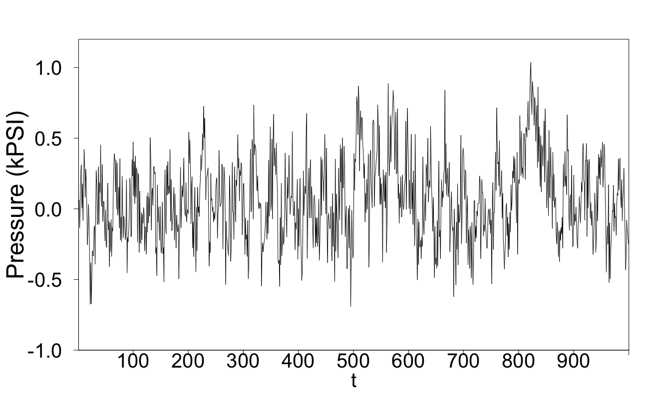
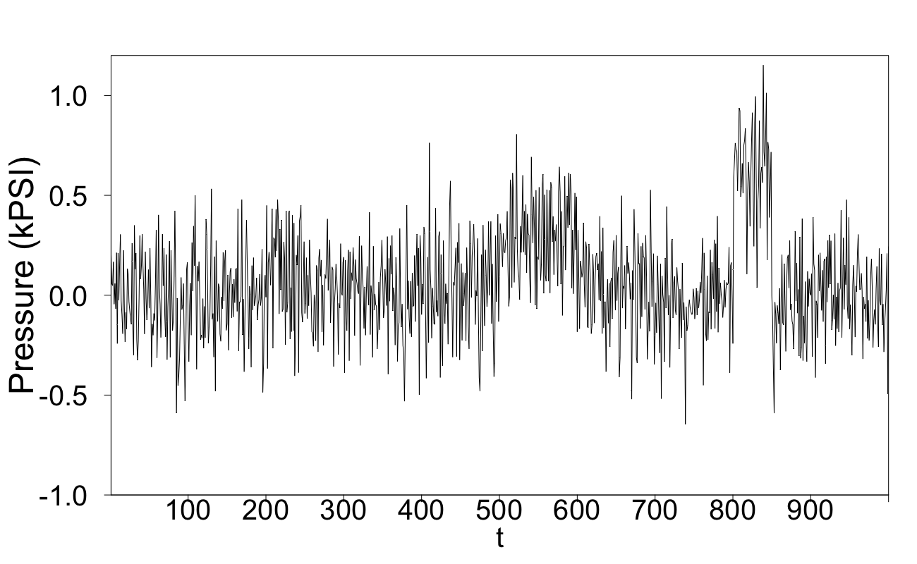
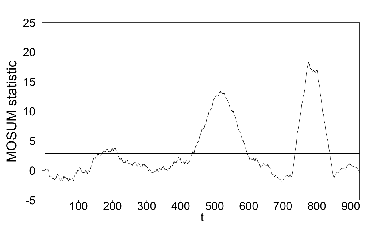
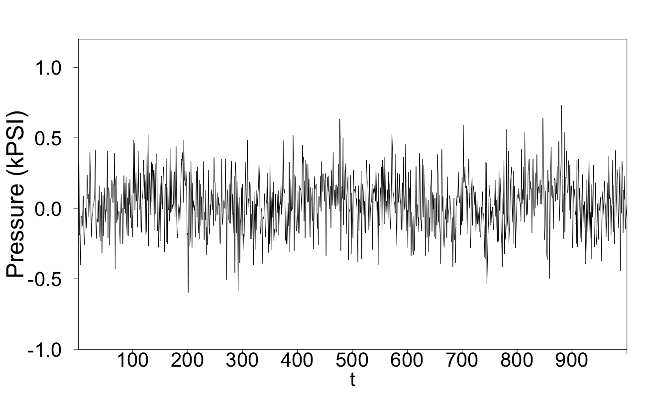
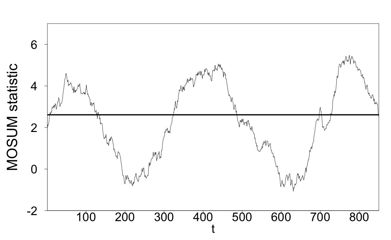
A sensible way of modelling the data under the null hypothesis of no pressure test could be , where represents the signal introduced by the wave motion and can be modelled as i.i.d. and reflects the random noise that is present in the system. In most scenarios, there is significant pre-test data so and can be estimated with great accuracy and therefore assumed known. How to estimate or in general how to remove all main components of a signal leaving only noise can be performed using Singular Spectrum Analysis, see [59, 60]. When a pressure test begins, this can be reflected with a change in mean of the ; that is, under a pressure test . The value of is often constant, but can differ between tests and is generally unknown. Each test can differ in duration but typical lengths vary between units of time. One has to detect a transient change in mean of . The behaviour of is shown in Figure 15. In Figure 16, we depict the MOSUM statistic setting . The horizontal line in this figure corresponds to the threshold required for an ARL of 5000. The MOSUM statistic indicates the location of three performed pressure tests and has the great advantage of not requiring knowledge when determining the ARL threshold unlike the generalised MOSUM and CUSUM procedures. A similar example is shown in Figures 17-18, where has been selected; three tests have been clearly located.
Acknowledgements
This work was partially supported by EPSRC grant EP/M024830.
References
- [1] M. Basseville and I. Nikiforov. Detection of Abrupt Changes: Theory and Application. Prentice-Hall Inc, 1993.
- [2] A. Tartakovsky, I. Nikiforov, and M. Basseville. Sequential analysis: Hypothesis testing and changepoint detection. CRC Press, 2014.
- [3] A. Zhigljavsky and A. Kraskovsky. Detection of abrupt changes of random processes in radiotechnics problems. St. Petersburg University Press, St. Petersburg, Russia.(in Russian), 1988.
- [4] V. Poor and O. Hadjiliadis. Quickest detection. Cambridge University Press, 2008.
- [5] W. Shewhart. Economic control of quality of manufactured product. Macmillan And Co Ltd, London, 1931.
- [6] E. Page. Continuous inspection schemes. Biometrika, 41(1/2):100–115, 1954.
- [7] A. Shiryaev. On optimum methods in quickest detection problems. Theory of Probability & Its Applications, 8(1):22–46, 1963.
- [8] S. Roberts. A comparison of some control chart procedures. Technometrics, 8(3):411–430, 1966.
- [9] S. Roberts. Control chart tests based on geometric moving averages. Technometrics, 42(1):97–101, 2000.
- [10] G. Lorden. Procedures for reacting to a change in distribution. The Annals of Mathematical Statistics, 42(6):1897–1908, 1971.
- [11] G. Moustakides. Optimal stopping times for detecting changes in distributions. Annals of Statistics, 14(4):1379–1387, 1986.
- [12] M. Pollak. Optimal detection of a change in distribution. The Annals of Statistics, pages 206–227, 1985.
- [13] Y. Ritov. Decision theoretic optimality of the CUSUM procedure. The Annals of Statistics, pages 1464–1469, 1990.
- [14] L. Gordon and M. Pollak. An efficient sequential nonparametric scheme for detecting a change of distribution. The Annals of Statistics, pages 763–804, 1994.
- [15] T. Lai. Sequential changepoint detection in quality control and dynamical systems. Journal of the Royal Statistical Society: Series B (Methodological), 57(4):613–644, 1995.
- [16] B. Guépié, L. Fillatre, and I. Nikiforov. Detecting a suddenly arriving dynamic profile of finite duration. IEEE Transactions on Information Theory, 63(5):3039–3052, 2017.
- [17] B. Guépié, L. Fillatre, and I. Nikiforov. Sequential detection of transient changes. Sequential Analysis, 31(4):528–547, 2012.
- [18] T. Lai. Control charts based on weighted sums. The Annals of Statistics, 2(1):134–147, 1974.
- [19] C. Chu, K. Hornik, and C. Kaun. MOSUM tests for parameter constancy. Biometrika, 82(3):603–617, 1995.
- [20] P. Bauer and P. Hackl. The use of MOSUMS for quality control. Technometrics, 20(4):431–436, 1978.
- [21] P. Bauer and P. Hackl. An extension of the MOSUM technique for quality control. Technometrics, 22(1):1–7, 1980.
- [22] J. Glaz, V. Pozdnyakov, and S. Wallenstein. Scan statistics: Methods and applications. Springer Science & Business Media, 2009.
- [23] J. Glaz, J. Naus, and X. Wang. Approximations and inequalities for moving sums. Methodology and Computing in Applied Probability, 14(3):597–616, 2012.
- [24] J. Noonan and A. Zhigljavsky. Power of the MOSUM test for online detection of a transient change in mean. Sequential Analysis, 39(2):269–293, 2020.
- [25] J. Noonan and A. Zhigljavsky. Approximations for the Boundary Crossing Probabilities of Moving Sums of Random Variables. Methodology and Computing in Applied Probability, 2020.
- [26] A. Zhigljavsky and J. Noonan. First passage times for Slepian process with linear and piecewise linear barriers. Extremes, pages 1–25, 2021.
- [27] M. Bell. Information theory and radar waveform design. IEEE Transactions on Information Theory, 39(5):1578–1597, 1993.
- [28] V. Poor. An introduction to signal detection and estimation. Springer Science & Business Media, 2013.
- [29] R. Streit and P. Willett. Detection of random transient signals via hyperparameter estimation. IEEE transactions on signal processing, 47(7):1823–1834, 1999.
- [30] L. Schmerr. Fundamentals of ultrasonic nondestructive evaluation. Springer, 2016.
- [31] A. Bianchi, L. Mainardi, E. Petrucci, M. Signorini, M. Mainardi, and S. Cerutti. Time-variant power spectrum analysis for the detection of transient episodes in HRV signal. IEEE Transactions on Biomedical Engineering, 40(2):136–144, 1993.
- [32] V. Moskvina and A. Zhigljavsky. An algorithm based on Singular Spectrum Analysis for change-point detection. Communications in Statistics—Simulation and Computation, 32(2):319–352, 2003.
- [33] E. Brodsky and B. Darkhovsky. Nonparametric methods in change point problems, volume 243. Springer Science & Business Media, 2013.
- [34] P. Fryzlewicz. Wild binary segmentation for multiple change-point detection. Annals of Statistics, 42(6):2243–2281, 2014.
- [35] H. Cho and P. Fryzlewicz. Multiple-change-point detection for high dimensional time series via sparsified binary segmentation. Journal of the Royal Statistical Society: Series B: Statistical Methodology, pages 475–507, 2015.
- [36] K. Korkas and P. Fryzlewicz. Multiple change-point detection for non-stationary time series using wild binary segmentation. Statistica Sinica, pages 287–311, 2017.
- [37] P. Fryzlewicz. Detecting possibly frequent change-points: Wild Binary Segmentation 2 and steepest-drop model selection. Journal of the Korean Statistical Society, 49(4):1027–1070, 2020.
- [38] H. Dette and J. Gösmann. A likelihood ratio approach to sequential change point detection for a general class of parameters. Journal of the American Statistical Association, 115(531):1361–1377, 2020.
- [39] J. Gösmann, T. Kley, and H. Dette. A new approach for open-end sequential change point monitoring. arXiv preprint arXiv:1906.03225, 2019.
- [40] A. Polunchenko, A. Tartakovsky, and N. Mukhopadhyay. Nearly optimal change-point detection with an application to cybersecurity. Sequential Analysis, 31(3):409–435, 2012.
- [41] D. Siegmund. Sequential Analysis: Tests and Confidence Intervals. Springer, 1985.
- [42] G. Moustakides, A. Polunchenko, and A. Tartakovsky. Numerical comparison of cusum and shiryaev–roberts procedures for detecting changes in distributions. Communications in Statistics—Theory and Methods, 38(16-17):3225–3239, 2009.
- [43] A. Tartakovsky. Asymptotic performance of a multichart CUSUM test under false alarm probability constraint. In Proceedings of the 44th IEEE Conference on Decision and Control, pages 320–325. IEEE, 2005.
- [44] M. Pollak. Average run lengths of an optimal method of detecting a change in distribution. The Annals of Statistics, pages 749–779, 1987.
- [45] T. Lai. Information bounds and quick detection of parameter changes in stochastic systems. IEEE Transactions on Information Theory, 44(7):2917–2929, 1998.
- [46] A. Tartakovsky. Discussion on “is average run length to false alarm always an informative criterion?” by Yajun Mei. Sequential Analysis, 27(4):396–405, 2008.
- [47] B. Levin and J. Kline. The CUSUM test of homogeneity with an application in spontaneous abortion epidemiology. Statistics in Medicine, 4(4):469–488, 1985.
- [48] D. Siegmund. Boundary crossing probabilities and statistical applications. The Annals of Statistics, pages 361–404, 1986.
- [49] M. Hogan and D. Siegmund. Large deviations for the maxima of some random fields. Advances in Applied Mathematics, 7(1):2–22, 1986.
- [50] D. Siegmund. Approximate tail probabilities for the maxima of some random fields. The Annals of Probability, pages 487–501, 1988.
- [51] Q. Yao. Large deviations for boundary crossing probabilities of some random fields. In Journal of Mathematical Research and Exposition, volume 9, pages 181–192, 1989.
- [52] Q. Yao. Tests for change-points with epidemic alternatives. Biometrika, 80(1):179–191, 1993.
- [53] D. Slepian. First passage time for a particular Gaussian process. The Annals of Mathematical Statistics, 32(2):610–612, 1961.
- [54] L. Shepp. First passage time for a particular Gaussian process. Ann. Math. Stat., 42(3):946–951, 1971.
- [55] J. Noonan and A. Zhigljavsky. Approximating Shepp’s constants for the Slepian process. Statistics & Probability Letters, 2019.
- [56] C. Han, P. Willett, and D. Abraham. Some methods to evaluate the performance of Page’s test as used to detect transient signals. IEEE transactions on signal processing, 47(8):2112–2127, 1999.
- [57] B. Bakhache and I. Nikiforov. Reliable detection of faults in measurement systems. International Journal of adaptive control and signal processing, 14(7):683–700, 2000.
- [58] S. McAleese. Operational aspects of oil and gas well testing. Elsevier, 2000.
- [59] N. Golyandina, V. Nekrutkin, and A. Zhigljavsky. Analysis of Time Series Structure: SSA and related techniques. Chapman & Hall/CRC, 2001.
- [60] N. Golyandina and A. Zhigljavsky. Singular Spectrum Analysis for time series. Springer, 2020.