Fermion masses and mixings, dark matter, leptogenesis and muon anomaly in an extended 2HDM with inverse seesaw.
Abstract
We propose a predictive flavored 2HDM model, where the scalar sector is enlarged by the inclusion of several gauge singlet scalars and the fermion sector by the inclusion of right handed Majorana neutrinos. In our model, the family symmetry is supplemented by several auxiliary cyclic symmetries, whose spontaneous breaking produces the observed pattern of SM charged fermion masses and quark mixing angles. The light active neutrino masses are generated from an inverse seesaw mechanism at one loop level thanks to a remnant preserved symmetry. Our model succesfully reproduces the measured dark matter relic abundance and is consistent with direct detection constraints for masses of the DM candidate around 6.3 TeV. Furthermore, our model is also consistent with the lepton and baryon asymmetries of the Universe as well as with the muon anomalous magnetic moment.
I Introduction
Despite of being a highly successful theory in describing the electromagnetic, strong and weak interactions, whose predictions have been verified with the greatest degree of accuracy by the experiments at the Large Hadron Collider (LHC), the SM model has several drawbacks. It fails in providing a natural explanation for the very large hierarchy in the fermion sector, which spans over a range of 13 orders of magnitude from the light active neutrino mass scale up to the top quark mass. Furthermore the observed pattern of fermion mixings characterized by small quark mixing angles and sizeable leptonic mixing ones does not find an explanation within the context of the SM. Besides that, the observed amount of dark matter relic density of the universe and lepton asymmetry are not addressed by the SM. These unaddressed issues motivate to consider extensions of the SM model with augmented particle spectrum and extended symmetries. Discrete flavor symmetries have been shown to be very useful in successfully describing the observed pattern of SM fermion masses and mixings. Some reviews of discrete flavor groups are provided in King:2013eh; Altarelli:2010gt; Ishimori:2010au; King:2015aea. In particular, the discrete flavor groups having small amount of doublets and singlets in their irreducible representations, such as, for example Lovrekovic:2012bz; Vien:2019lso and Frampton:1994rk; Grimus:2003kq; Grimus:2004rj; Frigerio:2004jg; Blum:2007jz; Adulpravitchai:2008yp; Ishimori:2008gp; Hagedorn:2010mq; Meloni:2011cc; Vien:2013zra; Vien:2014ica; Vien:2014soa; CarcamoHernandez:2020ney; Vien:2020uzf; Bonilla:2020hct have been implemented in extensions of the SM since they allow to provide an economical and simple way for obtaining viable fermion mass matrix textures, then allowing to successfully explain and accommodate the current pattern of SM fermion masses and mixings. Furthermore, several theories with extended symmetries and particle spectrum have also been proposed to find an explanation for the muon anomalous magnetic moment, see Athron:2021iuf for a very recent review. This muon anomaly was recently confirmed by the Muon experiment at FERMILAB Abi:2021gix and is one of the motivation for considering extensions of the SM.
In the present paper, we propose an extended 2HDM with enlarged particle spectrum where the SM gauge symmetry is supplemented by the family symmetry together with other auxiliary symmetries, thus allowing to get predictive textures for the SM fermion sector consistent with the low energy SM fermion flavor data. In the proposed model, the SM charged fermion mass and quark mixing pattern is generated by the spontaneous breaking of the discrete symmetries and the light active neutrino masses are produced by a radiative inverse seesaw mechanism at one loop level, thanks to a remnant preserved symmetry. To the best of our knowledge our proposed model is the first flavoured theory with radiative inverse seesaw mechanism where a cobimaximal mixing pattern governs the lepton mixings and the discrete symmetries yield extended Gatto-Sartori-Tonin relations between the quark masses and mixing angles. Furthermore, unlike other works about models with discrete flavor symmetry mostly focused in the implications of fermion masses and mixings, mainly in the lepton sector, in our current work we analyze in detail the consequences of our model in fermion masses and mixings, muon electric dipole and anomalous magnetic moments, dark matter and leptogenesis. In this way, under certain assumptions we attempt to solve several problems in one single flavor model. While these assumptions are meant to lessen the complexity of the model, they are well motivated and allow for a thorough analysis of several aspects of it. Concretely, in the matter sector, the only assumption is made in the neutrino sector, where we assume the equality of a pair of Yukawa couplings in order to get a light active neutrino mass matrix featuring the cobimaximal mixing pattern of lepton mixings, which is consistent with the neutrino oscillation experimental data. Regarding the quark sector no assumption is made and the extended Gatto-Sartori-Tonin relations are a direct consequence of the symmetries of the model and the particle assignments under the discrete and SM gauge groups. Likewise, in the treatment of the effective low energy scalar potential, while we give approximate analytical equations for the CP-even physical scalars we employ exact numerical algorithms during the scan of parameter space. For the phenomenology involving collider limits for scalars, we neglect the masses of the first and second family of fermions and also off-diagonal terms in the Yukawa matrices. Deviations of the matter sector with respect to the SM are expected to be of negligible influence when analyzing present collider limits on scalars.
The layout of the remainder of the paper is as follows. In section II we describe our extended 2HDM. Its implications on SM fermion masses and mixings are analyzed in section III. The consequences of our proposed theory in Dark matter, muon anomalous magnetic moment and leptogenesis are discussed in sections V, IV and VI, respectively. We conclude in section VII. Some technical details are given in the appendices. Appendix A provides a concise description of the discrete group. The scalar potential for two doublets is analyzed in Appendix B.
II The model
We propose an extended 2HDM where the scalar sector is augmented by the inclusion of several gauge singlet scalars and the fermion sector is extended by the inclusion of six right handed Majorana neutrinos. The SM gauge symmetry is extended by the inclusion of the discrete group, whose spontaneous breaking generates predictive fermion mass matrices consistent with the SM fermion masses and mixing parameters. The role of the aforementioned cyclic symmetries is explained in the following. The symmetry shapes the textures of the SM fermion mass matrices thus reducing the model parameters, especially in the SM lepton sector. We choose the symmetry since it is the smallest non-Abelian discrete symmetry group having five irreducible representations (irreps), explicitly, four singlets and one doublet irreps. Besides that, the flavour symmetry allows more freedom in assigning the fermionic and scalar fields in different representations and having more suppressed Yukawa interactions when compared with . Moreover, the discrete group has very similar tensor product rules as and thus using instead of will not yield significant changes in the model and the resulting physical results would be very similar to the ones corresponding to the flavoured theory. Replacing by the flavor group will only yield important modifications in the neutrino Yukawa terms, due to the fact that the right handed Majorana neutrinos are the only fermionic fields of the model assigned as doublets. This will affect the annihilation channels of fermionic dark matter candidates. Thus, the annihilation channels of the fermionic dark matter candidate , such as for instance () can be an experimental test to distinguish our flavored model from an alternative model based on the family symmetry.
The separates the two scalar doublets and , thus allowing to get viable and predictive quark mass matrix textures where the Cabbibo mixing arises from the down quark sector whereas the remaining quark mixing angles are generated from the up quark sector. On the other hand, the and discrete symmetries shape the hierarchical structure of the SM charged fermion mass matrices crucial to yield the observed pattern of SM charged fermion masses and mixing angles. The discrete symmetry is spontaneously broken to a preserved symmetry, which allows the implementation of one loop level inverse seesaw mechanism that produces the tiny masses for the light active neutrinos. The assignments for scalars, quarks and leptons are shown in Tables 1, 2 and 3, respectively. Here the different charges are given in additive notation. Let us note that a field transforms under the symmetry as: , , where is its corresponding charge in additive notation. As shown in Tables 1 and 3, the gauge singlet scalars () and the right handed Majorana neutrino are the only particles having a complex charge, corresponding to a nontrivial charge under the preserved symmetry. Due to the preserved symmetry our model has stable scalar and fermionic dark matter candidates. The scalar dark matter candidate is the lightest among and (), whereas the fermionic dark matter candidate is the gauge singlet neutral lepton .
| 0 | 1 | 0 | 0 | 0 | 0 | 0 | 1 | 1 | |
| 0 | 0 | 0 | -1 | 0 | 0 | 0 | 0 | 0 | |
| 0 | 0 | 0 | 0 | 0 | -1 | -1 | -2 | -2 | |
| 0 | 0 | -1 | 0 | 0 | -1 | -1 | 0 | 0 |
| 0 | 0 | 1 | 0 | 0 | 1 | 2 | 2 | 1 | |
| 0 | 0 | 0 | 0 | 0 | 0 | -1 | -1 | 1 | |
| 0 | 0 | 0 | 0 | 0 | 0 | 0 | 0 | 0 | |
| 0 | 0 | 0 | 4 | 2 | 0 | 4 | 2 | 2 |
| 0 | 0 | 0 | 0 | 0 | 1 | 1 | 1 | 2 | 2 | 1 | |
| 0 | 0 | 0 | 0 | 0 | 0 | 0 | 0 | 0 | 0 | 0 | |
| 0 | 0 | 0 | 0 | 0 | 0 | 0 | 0 | 0 | 0 | 1 | |
| 0 | 0 | 0 | 0 | 0 | 0 | 0 | 0 | 0 | 0 | 0 |
In order to get a predictive and viable pattern of SM fermion masses and mixings we consider the following vacuum expectation value (VEV) configuration for the doublets SM gauge singlet scalars and ;
| (1) |
Such VEV configuration is consistent with the scalar potential minimization equations for a large region of parameter space as shown in detail in Appendix B.
Given that the observed SM charged fermion mass and quark mixing pattern is caused by the spontaneous breaking of the discrete group, the vacuum expectation values (VEVs) of the gauge singlet scalars are set to fullfill the following hierarchy:
| (2) |
where GeV, is the Wolfenstein parameter and is the model cutoff. Notice that the gauge singlet scalar field is assumed to acquire a VEV at the TeV scale, in order to get TeV scale sterile neutrinos in the leptonic spectrum, thus allowing to have sterile neutrino signatures testable at colliders.
In what follows we provide a discussion about the different scales (2) of the vacuum expectation values of the singlet scalar fields. Notice that there is no symmetry that protects this pattern from large radiative corrections. Thus, in order to stabilize it, we need to apply certain tuning of the model parameters. The corresponding vacuum stability conditions arise from the Coleman-Weinberg type 1-loop effective potential. This analysis is left beyond the scope of the present paper. However, since in our model the VEV hierarchy (2) is rather moderate, not exceeding three orders of magnitude, we expect that the quadratic divergences dangerous for a strong hierarchy can be tamed here by a moderate tuning of the model parameters. At the same time, for the scales larger than in (2), where this is not possible, we proceed to assume that our model is embedded into a more fundamental theory with additional symmetries that protect the hierarchy up to the Planck scale. Some well-known and motivated examples of such theories are supersymmetry and warped five-dimensions.
The relevant Yukawa terms are:
| (3) | |||||
| (4) | |||||
| (5) | |||||
| (6) | |||||
where we have introduced the soft-breaking Majorana mass term in order to get the correct sign and magnitude of the muon anomalous magnetic moment. Other possible soft-breaking mass terms of the form and in the lepton sector will generate corrections to the submatrix of the block of the full neutrino mass matrix. These corrections will add extra contributions to the mass matrices of the light active and sterile neutrinos neutrinos, along the same lines of Law:2013gma. However such contributions are very subleading.
It is worth stressing that the flavor symmetry is more relevant in the lepton sector since some of the leptonic fields are assigned as doublets as seen in Table 3 and the considered setup allows to get a predictive light active neutrino mass matrix featuring the cobimaximal mixing pattern, as it will be shown in the next section. In the concerning to the quark sector, despite there are no doublets (as follows from Table 3), the importance of the flavor symmetry is that it allows to get, for example a twelve dimensional Yukawa operator crucial for a naturally explanation of the smallness of the up quark mass without relying on the inclusion of large cyclic symmetries like for instance . This is due to the fact that there is no scalar field in the particle spectrum assigned as and thus the effective scalar required to build the twelve dimensional Yukawa operator (last term of Eq. (3)) that generates the up quark mass term, is built from the quartic combination involving the scalar doublet . This trick is also used in the construction of the up type quark Yukawa operator (first term of Eq. (3)) that yields the quark mixing angle.
In what follows we will describe a plausible ultraviolet origin for these non-renormalizable operators. As seen from Eqs. (3), (4), (5) and (6), we introduced several non-renormalizable Yukawa operators. These allow us to explain the observed hierarchies in the SM fermion mass spectrum and the fermion mixing parameters while keeping all the Yukawa couplings of order unity. Notice that all of them have the following form:
| (7) |
where and stand for light and heavy fermions, respectively, , are integers and , , and are scalars. Here, for simplicity, we have omitted family and fermionic type indices. One sees that these non-renormalizable operators in Eq. (7) can all arise from the following renormalizable operators:
| (8) |
where () are extra scalars and extra very heavy fermions. Assuming that the and scalars acquire vacuum expectation values much larger than the remaining scalars, the fermions will get very large masses. As a result, they can be integrated out, yielding effective non-renormalizable operators as in Eq. (7). Now in order to make our discussion more explicit and we are going to specify a possible ultraviolet origin of the following non renormalizable neutrino Yukawa operators:
| (9) |
where we have suppressed the subscript of the scalar field , unessential for our discussion. These three non-renormalizable Yukawa terms of Eq. (9) can be generated at low energies by the Feynman diagrams shown in Figure 1 after integrating out the heavy scalar fields and with characteristic masses of the order of our model cutoff scale . Their assignment under the symmetries of the model is dictated by the requirement that the renormalizable interactions in the vertices of these diagrams be invariant under these symmetries.
Thus, it follows that , and are doublets, whereas is a singlet. Furthermore, is a scalar doublet with hypercharge (as the usual SM Higgs doublet), whereas , and are electrically neutral scalars transforming as singlets under the SM gauge symmetry.
On the other hand, the non renormalizable charged lepton Yukawa operators:
| (10) |
can be generated at low energies from the Feynman diagrams shown in Figure 2 after integrating out the heavy scalar fields , , , and with masses of the order of the model cutoff . Here the invariance of the above given Yukawa interactions under the flavor group requires that the fields and transform as doublets, whereas , and as singlets. Besides that, , and are scalar doublets with hypercharge and , are gauge singlet scalars. Note that the symmetries of the model ensure that the only presented operators are the ones that are generated in the UV completion of the non renormalizable leptonic interactions. The analysis of the evolution of the couplings with energies requires careful and detailed studies beyond the scope of the present work.
III Fermion masses and mixings
III.1 Quarks: masses and mixings
In the standard basis, the quark mass term is given as
| (11) |
where the quark mass matrices can be written as
| (12) |
where (), (), and are dimensionless parameters and is the Wolfenstein parameter. The above given SM quark mass matrices can be rewritten in the form:
| (13) |
In here, the coefficients may be read of Eq. (12). Then, the quark mass matrices are diagonalized by the mixing matrices where . Explicitly, we have where contains the physical quark masses.
As it is well known, the CKM mixing matrix is given by , then we will obtain the left-handed mixing matrix that takes place in the CKM matrix. Therefore, we have to build the bilineal forms so that let us start with the down sector. First of all, we factorize the CP violating phases that come from , this is, where with
| (14) |
In addition, we have
| (15) |
Three free parameters can be fixed in terms of the physical masses and one unfixed parameter, explicitly, these are given as
| (16) |
where . According to the parametrization, there is a hierarchy among the free parameters, this is,
Having done that, one can choose appropriately the left-handed mixing matrix . In here, is an orthogonal real matrix that diagonalizes .
| (17) |
with and .
In similar way, for the up sector, we have to factorize the CP violating phases that come from so that where . The phases are given as
| (18) |
with , and . At the same time, we have the real symmetric matrix
| (19) |
which has five free parameters. Three of them can be fixed in terms of the physical masses, and . Then, the fixed parameters are written as
| (20) |
where
| (21) |
With this parametrization, the hierarchy among the free parameters is . So that, the left-handed matrix is well determined as where the latter matrix diagonalizes the real symmetric matrix, . Explicitly, this is given by
| (22) |
with
| (23) |



Therefore, the CKM mixing matrix is written as where with . In summary, the theoretical CKM matrix depends of five parameters namely: , , and two CP phases. From these five parameters, four of them have to be numerically determined with high precision in order to get values for the CKM parameters consistent with the experimental data, as follows from our numerical analysis. Only the phase can be varied in larger range when searching for the best point that reproduces the observed CKM mixing.
Remarkably, the phase is irrelevant for the magnitude of each entry of the third column. This facts will allow to reduce the free parameters so that four of them can be fitted. Before starting an analysis, we show that in this model, the extended Gatto-Sartori-Tonin relations, are consequence of the hierarchical structure of the quark mass matrices, resulting from the symmetries of the model, which imply . As result, one gets
| (24) |
Regarding, the up sector, the hierarchical structure of the up quark mass matrix implies that the free parameters must be and with . In this way, we respect the hierarchy among the free parameters. Therefore, after a lengthy task, the following relations are obtained
| (25) |
After the above given analytical analysis of the quark spectrum and CKM mixing matrix we carry out a numerical analysis. From this analysis we find that the experimental values of the quark mass spectrum and CKM parameters can be very well reproduced from the following benchmark point:
| (26) |
An important feature of the above result is that the absolute values of all these parameters are of the order of unity. Thus, the symmetries of our model allow us to naturally explain the hierarchy of quark mass spectrum and quark mixing angles without appreciable tuning of these effective parameters.
| Observable | Model value | Experimental value |
|---|---|---|
The result given in Eq. (26) motivates to consider the simplified benchmark scenario:
As seen from Table 5, the 10 quark observables are reproduced with a good precision in the above given 7-parameter scenario.
| Observable | Model value | Experimental value |
|---|---|---|
To close this section, we briefly discuss the implications of our model in Flavour Changing Neutral Currents (FCNC). As seen from the charged fermion Yukawa terms of Eqs. (3), (4), (5), there is only one Higgs doublet appearing in the charged lepton and down type quark Yukawa interactions, thus implying the absence of FCNC at tree level, as follows from the Weinberg-Glasgow-Pascos theorem. Consequently, we expect similar predictions for the , and meson mixings as in the Standard Model. On the other hand, there are two Higgs doublets in the up type quark Yukawa interactions, thus implying the appearance of tree level FCNC in the up type quark sector that will yield a tree level contribution mediated by neutral scalars to the meson oscillation. However, we expect that the strong hierarchical structure in the Yukawa couplings of the neutral scalars with up type quarks together with the very small mixing between the first and second family of up type quarks, will provide a strong suppression for the tree level contribution to the meson mixing.
III.2 Lepton masses and mixings
From the charged lepton Yukawa interactions, we find that the SM charged lepton mass matrix reads:
| (30) |
The above given charged lepton mass matrix can be rewritten as:
| (31) |
Then, in similar way to the down quark sector, three free parameters may be fixed in terms of the physical masses and the unfixed parameter, . This is
| (32) |
where . In this case, the free parameters satisfy the following ordering
Along with this, left-handed matrix that takes places in the PMNS mixing matrix is given by with
| (33) |
with and ; where and .
Regarding the neutrino sector, from the Eq. (6), we find the following neutrino mass terms:
| (34) |
where the neutrino mass matrix is given by:
| (35) |
and the submatrices are given by:
where , () and for the sake of simplicity, we have assumed that the singlet scalar fields are physical fields degenerate in mass and heavier than the right-handed Majorana neutrino , thus allowing to consider the scenario
| (50) |
Furthermore, we have assumed as well as GeV. The block is generated at one loop level due to the exchange of , and in the internal lines, as shown in figure 4. To close the corresponding one loop diagram, the following non renormalizable scalar interactions are needed:
| (51) |
such interaction generates a small splitting between the masses and , which is crucial to produce the tiny masses for the light active neutrinos. Taking into account the VEV hierarchy given in Eq. (2), this small splitting can be estimated as follows:
| (52) |
where the exact values depend on the specific magnitudes of the VEVs of the scalar singlets as well as of the quartic scalar couplings (). These quartic scalar couplings can take values up to their upper perturbativity bound of .
The light active masses arise from an inverse seesaw mechanism and the physical neutrino mass matrices are:
| (53) | |||||
| (54) | |||||
| (55) |
where corresponds to the mass matrix for light active neutrinos (), whereas and are the mass matrices for sterile neutrinos () which are superpositions of mostly and as . In the limit , which corresponds to unbroken lepton number, the light active neutrinos become massless. The smallness of the - parameter makes the mass splitting of three pairs of sterile neutrinos to become small, thus implying that the sterile neutrinos form pseudo-Dirac pairs.
From Eqs. (III.2) and (53), we find that the light active neutrino mass matrix takes the form:
| (60) |
The above given effective neutrino mass matrix, in the simplified benchmark scenario can be written as:
| (61) |
where and . This matrix is diagonalized by the mixing matrix , this is, with . As it has been shown, the neutrino mixing matrix is parametrized by . Explicitly, we have
| (62) |
In the above matrices, () are unphysical phases; () stands for the Majorana phases. In addition, there are three angles and one phase that parameterize the rotations.
As one can verify, the and phases are not arbitrary since they can be fixed by inverting the expression, to obtain the effective mass matrix. This means explicitly, , then, we obtain
| (63) |
These matrix elements are obtained with and ; and . Along with these, and .
Having given the above conditions, let us write explicitly the neutrino mixing matrix
| (64) |
Therefore, the PMNS mixing matrix is given by where denotes the normal and inverted hierarchy, respectively.
In here, we add a important comment on the matrix. If the charged lepton mass matrix was diagonal, then the matrix would be identified with the well known cobimaximal mixing matrix. In the current model, the charged lepton is not diagonal so that we expect some deviations to cobimaximal mixing matrix.
The expression for the mixing angles are obtained by comparing our PMNS mixing matrix with the standard parametrization. Then, one obtains
| (65) |
We ought to comment that there are still free parameters in the PMNS mixing matrix namely: (or ), , and the phase . As we notice, with , the Cobimaximal predictions are recovered: and the CP-violating phase, . A numerical analysis has to be done to constrain those parameters.
In addition, one gets for the Jarlskog invariant
| (66) | |||||
Here, we want to show explicitly that the CP-violating phase, , is deviated from by the charged lepton sector. To do this, we perform an approximation as follows: let us consider in the charged lepton mass matrix, which implies and . Then, we obtain the following PMNS matrix elements
| (67) |
Having done that, using the Jarlskog invariant one obtains
where
therefore
| (68) |
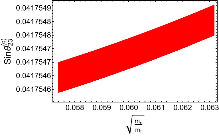
In the above expression, we could consider in good approximation. In addition, in the already mentioned approximation so that the Dirac CP phase is near to . The correlations of the atmospheric with the reactor mixing angle and with the leptonic Dirac CP violating phase are shown in figure 5.


IV Muon anomalous magnetic moment
In this section we will discuss the consequences of our model in the muon anomalous magnetic moment. The dominant contribution to the muon anomalous magnetic moment arises from the one-loop diagram involving the exchange of electrically charged scalars and nearly degenerate sterile neutrinos running in the internal lines. Unlike the model of Mondragon:2007nk, the muon anomalous magnetic moment does not receive contributions involving electrically neutral virtual scalars since in our model only one scalar doublet participates in the charged lepton Yukawa interactions, which prevents the appearance of flavor changing neutral scalar interactions in the lepton sector. Then, in our model the leading contribution to the muon anomalous magnetic moment is given by:
| (69) |
where loop integral has the form Diaz:2002uk; Jegerlehner:2009ry; Kelso:2014qka; Lindner:2016bgg; Kowalska:2017iqv
| (70) |
where
| (71) |
Considering that the muon anomalous magnetic moment is constrained to be in the range Hagiwara:2011af; Davier:2017zfy; Blum:2018mom; Keshavarzi:2018mgv; Nomura:2018lsx; Nomura:2018vfz; Aoyama:2020ynm; Abi:2021gix:
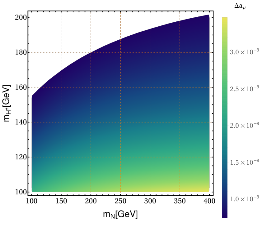
We plot in figure 6 the allowed parameter space in the plane consistent with the muon anomalous magnetic moment. We have fixed , , , GeV. Notice that the complex phases in the couplings and can be rotated away by a phase redefinition of the right handed Majorana neutrino fields. Consequently, the couplings and can be taken real without a loss of generality. It is worth mentioning that the range of values for charged scalar masses is consistent with the collider constraints Sanyal:2019xcp; CMS:2020osd. We find that our model can successfully accommodate the experimental values of the muon anomalous magnetic moment. On the other hand, there is an extra two loop level contribution to the muon anomalous magnetic moment arising from the Barr-Zee type mechanism Arhrib:2001xx, however we have numerically checked that this contribution is of the order of for electrically charged scalar masses of about GeV and quartic scalar couplings of order unity. It is worth mentioning that in the case where the muon anomaly does not get confirmed, the electrically charged scalars will have masses close to the TeV scale.
On the other hand, CP-violating interactions related to the Barr-Zee two-loop mechanism can give rise values of the muon electric dipole moment, several orders of magnitude larger than the SM prediction Barr:1990vd; Chang:1998uc; Heo:2008sr; Heo:2008dq. In our model, the CP violating interactions responsible for the generation of the muon electric dipole moment only appear when one consider complex quartic scalar coupling, which corresponds to a CP violating scalar potential. In that case, these CP violating interactions are:
and the resulting two loop level induced muon electric dipole moment has the form:
where the two loop integral has the form:
| (72) |
Figure 7 displays the muon electric dipole moment as a function of the CP odd scalar mass , for different values of the charged scalar masses, taken to be equal to GeV, GeV, GeV and GeV, for the black, blue, magenta and orange curves, respectively. As shown in figure 7, the muon electric dipole moment reach values around e.cm, which is several orders of magnitude larger than the SM prediction e.cm muonEDMinitiative:2022fmk. Besides that, our obtained values of the muon electric dipole moment are lower than the experimental upper limit of e.cm. Note that the electric dipole moment obtained in our model is larger than zero provided that the scalar coupling is positive. We have numerically checked the two loop integral of Eq. (72) is always negative.
V Scalar and dark matter sectors
In this section we discuss the scalar and Dark Matter (DM) sectors of the model with more detail. We present several numerical results based on a scan of the parameter space of the model where we construct likelihood profiles involving observables of interest by comparing predictions with experimental measurements. A complete composite likelihood global analysis is outside the scope of this letter. We limit ourselves to include the information from the measured values of the relic density , Higgs mass and Baryon asymmetry of the Universe (BAU) as basic Gaussian likelihoods , and respectively. We also include a likelihood function based on recent results from the XENON1T Direct Detection Experiment, we then maximize over the model’s parameter space the composite log-likelihood
| (73) |
Note that in the high statistic limit, twice the negative of the composite log-likelihood approaches a -square function so this procedure is equivalent to minimizing such function. In the next subsections we detail the construction of these likelihood profiles.
Using such variety of physical observables to construct the total log-likelihood leads to a large number of free parameters, in our case we need 2711 1 In addition to the parameters of the mass and mixing matrices from the quark and charged lepton sector, which are kept fixed in the analysis of the scalar and DM sectors (the neutrino sector parameters influence the baryon asymmetry observable). to properly conduct the numerical analysis, however distinct observables depend mostly on different subsets of the free parameters. From inspection of the analytic equations for the predicted observables it is clear that only a few number of the free parameters have influence in all the physical observables considered, and this leads to important correlations between them.
V.1 Scalar mass spectra
For the purpose of this section, we will consider that all scalars which have VEVs of order of the model cutoff are decoupled, since their masses will be around that of the cutoff scale. This leaves us with an effective scalar potential . For simplicity we will assume that only the and scalar singlets couple to the Higgses and write the low energy scalar potential as . For the doublets and we’ll take the simple CP-conserving potential given by:
| (74) | |||||
with all parameters real. In order to reduce the number of free parameters for the numerical calculations, for the second part of the scalar potential we will take simply:
| (75) | |||||
Note that after Electroweak Symmetry Breaking (EWSB), the above scalar potential induces a mixing between the neutral scalar components of and and the singlet . As a result the field content of the model arises from the three field mass eigenstates from this mixing: , and , together with the pseudo scalar and the electrically charged scalar . The minimization conditions for this potential take the form:
| (76) | |||||
where is short for and as before . From these, we eliminate , and in terms of the remaining parameters, this however only means we would be sitting in an extremum of the potential. To ensure that the values of the parameters correspond in fact to a minimum, we check numerically during the scan of parameter space the stability of the potential at a given point using the public tool EVADE Ferreira:2019iqb; Hollik:2018wrr, which features the minimization of the scalar potential through polynomial homotopy continuation and an estimation of the decay rate of a false vacuum. We apply a hard cut on the parameter points that do not satisfy the stability criteria.
From the scalar potential we obtain the mass matrices for the different scalar particles. The charged and pseudoscalar cases contain the two SM massless Goldstone states (the longitudinal modes of the SM massive gauge bosons). The physical particles have masses given by:
| (77) |
| (78) |
For the CP-even neutral scalars we can write the mass matrix as:
| (79) |
with
| (80) | |||||
The neutral scalar mass matrix is diagonalized by the mixing matrix such that
| (82) |
We find for the masses22 2 These expressions are not general in the sense that they are not valid for cases where there are degenerate eigenvalues or when one or more of the matrix entries are zero, these atypical cases should be treated separately. In particular, these equations are not expected to reduce to the correct results in the limit , which is not contemplated since in this case four matrix entries reduce to zero. In the parameter scan we use standard numerical algorithms to diagonalize the mass matrices. deledalle:hal-01501221:
| (83) | |||||
where
| (84) |
and
| (85) |
with
| (86) | |||||
Note that so is always grater than but can be smaller than , this is an attractive feature of the model since there are some potential excesses in searches for light Higgs bosons reported by CMSCMS:2018cyk, nevertheless a detailed study of this matter is outside the scope of this work. We do take into account experimental constraints from scalar searches at colliders using the public tool HiggsBoundsBechtle:2020pkv and applying a hard cut on parameter space points not complying with these limits33 3 For this part of the numerical scan we neglect the masses of the first and second generation of fermions and neglect off-diagonal entries in the Yukawa matrices. We expect deviations of the matter sector relative to the SM to be of negligible influence in the phenomenology of the scalar sector at present collider searches. .
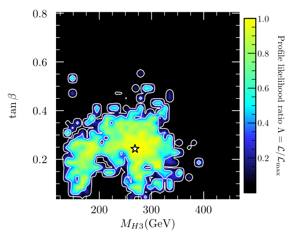
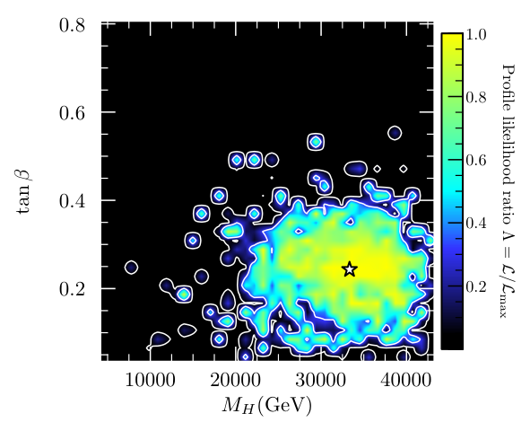
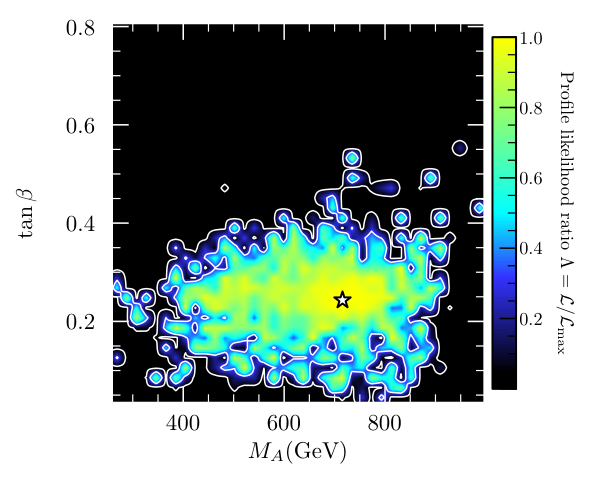
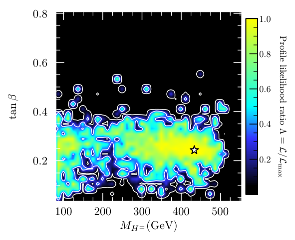
In figure (8) we present the low energy scalar mass spectra of the model, the regions of parameter space that better match high values of the composite log-likelihood are shown as bright zones, and the best fit point (BFP) is marked with a star. For the best fit point we find that Eq. (86) is negative and in turn is very close to . We thus find that the scalar is markedly heavier than which is around twice as heavy as the SM-like higgs . Note that preferred values of the charged scalar mass are around 400 GeV, however there are zones that also have high values of the likelihood function below 200 GeV.
V.2 Relic density
We will continue to assume that the components of the odd fields () are heavier than the DM Majorana fermion and thus consider the latter as our DM candidate44 4 A second case, namely that one of the fields be the lightest of the DM particles is of course also possible leading to a scalar DM candidate. In this letter we focus our attention on the fermion DM candidate in part because of a matter of taste and in part because of the demanding computational times required for the numerical analysis which make unfeasible to present both cases in a single piece. We restrict our analysis to the scenario of fermionic Dark Matter only, because the case of scalar dark matter candidate is a bit generic and our expected results will be similar to those ones discussed in Abada:2021yot; Hernandez:2021zje; Espinoza:2018itz, where the dark matter constraints set the mass of scalar dark matter candidates larger than about few TeVs or in a small window close to the half of the SM Higgs boson mass. Besides that, one can also consider the scenario of multicomponent dark matter candidates, however such scenario requires carefull analysis which are beyond the scope of the present work. . Since the only interaction of that is not suppressed by the cutoff is the one involving the Yukawa coupling , it follows that the DM observables will mostly depend on its mass, the coupling and the mass of the mediators. In the region of the parameter space where the couplings of to the scalars are small, will be “mostly” , but in general the DM candidate will communicate with the visible sector through all the above scalar mass eigenstates.
For the numerical calculation of the relic density, the cutoff is taken as TeV and we keep the masses of the components of () large ( 50 TeV) but with a small mass splitting between them to ensure that the parameter influencing the masses of the active neutrinos is of order eV so that not much fine tunning of the neutrino Yukawa couplings would be required. It is worth mentioning that a naturally small mass splitting can arise from the higher-dimensional operators of Eq. (51), as discussed in the previous section.
Finally, we implement the model in SARAH Staub:2008uz; Staub:2009bi; Staub:2010jh; Staub:2012pb; Staub:2013tta from which we obtain the Micromegas Belanger:2013oya; Belanger:2014vza; Barducci:2016pcb; Belanger:2018ccd model files to compute the value of the relic density and we perform a scan of the parameter space using Diver Workgroup:2017htr (in standalone mode).
In figure (9) we present the likelihood profile as a function of the mass of the DM candidate and its relic density (but not including the likelihood from the relic density, the corresponding plot with the full log-likelihood is just a slim horizontal bright band around the Planck measured value). We infer from this figure that DM candidate masses below TeV, though they can be compatible with e.g. direct detection limits, they would be overproduced at the freeze out epoch. We observed also that, assuming the DM candidate comprises 100% of the dark matter of the universe, its mass can only be around and TeV.

V.3 Direct detection
From the details brought up previously and inspecting the model’s Lagrangian, the DM candidate couples to fermions thanks to the mixing between the scalars. For simplicity we will assume the DM Yukawa coupling to be real, then the only parity conserving effective DM-quark interactions mediated by the physical scalars take the general form:
| (87) |
where the sums are over the quark fields and the physical scalars . The effective couplings and are functions of the free parameters and can be obtained explicitly from the Feynman rules of the model, we find ( and no summation over repeated indices):
| (88) |
and for and type quarks:
| (89) |
while for and quarks we have:
| (90) | |||||
where we have denoted the quark mixing matrices by to avoid index cluttering. The quark Yukawa couplings are obtained from the benchmark point (26) using the relations:
| (91) |
| (92) |
From these we obtain the DM-nucleon differential scattering cross section (in the nonrelativistic limit):
| (93) |
here is the nucleon recoil energy, the nucleon mass and the DM velocity. The scattering amplitude (averaged over initial spins and summed over final spins) receives the contribution of three diagrams (one for each scalar mediator) of the form:
| (94) |
where and denote DM and nucleon spin indices respectively, is the momentum transfer, the mass of the scalar mediators and is defined as
| (95) |
with the quark valence masses and expresses the quark-mass contributions to the nucleon mass. Numerical values for the latter can be found e.g. in DelNobile:2021icc and references therein. The momentum transfer is related to the recoil energy through , so that the total DM-nucleon spin independent cross section reads:
| (96) |
with the maximum recoil energy given by
| (97) |
being the DM-nucleon reduced mass.
We now present a likelihood analysis involving publicly available data from the direct detection XENON1T experiment XENON:2018voc. We make use of the capabilities of the numerical tool DDCalc to compute the Poisson likelihood given by
| (98) |
where is the number of observed events in the detector and is the expected background count. From the model’s predicted DM-nucleon cross sections Eq. (96) as input, DDCalc computes the number of expected signal events for given DM local halo and velocity distribution models (we use the tool’s default models, for specific details on the implementation such as simulation of the detector efficiencies and acceptance rates, possible binning etc. see GAMBITDarkMatterWorkgroup:2017fax; GAMBIT:2018eea).
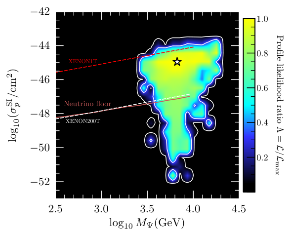
In figure (10), we present the profile likelihood normalized to the value of at the best fit point (signaled by a star) assuming the DM candidate constitutes 100% of the DM in the Universe. The plot shows the dependence of the likelihood on the DM mass and the DM-proton spin independent (SI) cross section; contours of 68% and 95% of confidence level (CL) are drawn. We also depict the 90% CL upper limit on the SI cross section from the XENON1T (1t yr) experiment XENON:2018voc, alongside with the multi ton-scale time projection to 200 t yr of reference55 5 For better comparison with the other curves we extrapolated linearly the data available from this reference from 1 TeV up to 10 TeV. Schumann:2015cpa and an estimation of the neutrino floor Billard:2013qya.
We note that almost all the region consistent with the constraints including the BFP lies below the zone currently excluded by the XENON1T experiment. However the figure also makes it evident that the multi ton projection to 200t1yr will be capable of probing zones well below the BFP of the model.
VI Leptogenesis
In this section we will analyze the implications of our model in leptogenesis. Here we consider the case where and . Therefore only the first generation of sterile neutrinos () can contribute to the Baryon asymmetry of the Universe. We further assume that the gauge singlet neutral lepton is heavier than the lightest pseudo-Dirac fermions . Then, the lepton asymmetry parameter, which is induced by decay process of , is given by Gu:2010xc; Pilaftsis:1997jf:
| (99) | |||||
| (100) |
with:
| (101) | |||||
| (102) |
Neglecting the interference terms involving the two different sterile neutrinos , the washout parameter is huge as mentioned in Dolan:2018qpy. However, the small mass splitting between the pseudo-Dirac neutrinos leads to a destructive interference in the scattering process Blanchet:2009kk. The washout parameter including the interference term has the following form:
| (103) |
where:
| (104) |
where is the number of effective relativistic degrees of freedom, GeV is the Planck constant and .
In the weak and strong washout regimes, the baryon asymmetry is related to the lepton asymmetry Pilaftsis:1997jf as follows
| (105) | |||||
| (106) |
The correlation of the baryon asymmetry parameter with the solar mixing angle for the weak washout regime is shown in figure 11. Our findings indicate that our model successfully accommodates the experimental value of the baryon asymmetry parameter :
| (107) |


Figure 11 shows the allowed values of the baryon asymmetry parameter , leptonic mixing angles and the mass of the lightest pseudoDirac neutral lepton pair for the weak washout regime. We find that the consistency with lepton masses and mixings, dark matter and baryon asymmetry constraints requires values for the leptonic mixing angles in the ranges , , as well as a mass for the lightest heavy pseudo Dirac neutral lepton pair at the subTeV scale.
VII Conclusions
We have built a predictive and viable extended 2HDM, where the scalar and fermion sectors are enlarged by the inclusion of gauge singlet scalars and right handed Majorana neutrinos, respectively. The model incorporates the family symmetry, which is supplemented by several auxiliary cyclic symmetries, which allows to successfully describe the current pattern of SM fermion masses and mixing angles, which is caused by the spontaneous breaking of the discrete symmetries. The tiny masses of the light active neutrinos are produced by an inverse seesaw mechanism at one loop level, due to a remnant preserved symmetry resulting from the spontaneous breaking of the discrete group. Under certain simplifying assumptions made in the scalar and neutrino sectors (equality of a pair of Yukawa couplings) and described in detail in the introduction and throughout the text, our model successfully accommodates the experimental value of the dark matter relic density, the muon anomalous magnetic moment as well as the lepton and baryon asymmetries of the Universe. The consistency of our model with the constraints arising from collider searches for heavy scalars, stability of the scalar potentials, the dark matter relic density and current and future direct detection experiments sets the mass of the scalar dark matter candidate to be in between TeV and TeV. Finally our current flavor model intends to address and connect several problems such as the SM flavor puzzle, the current amount of dark matter and baryon asymmetries observed in the Universe, the muon anomalous magnetic moment. It predicts extended Gatto-Sartori-Tonin relations between the quark masses and mixing angles, a baryon asymmetry parameter between and , leptonic mixing angles in the following ranges , , , the mass of the lightest heavy pseudo Dirac neutral lepton pair at the subTeV scale, the parameter in the range and heavy non SM scalars at the subTeV scale with masses in the ranges GeV GeV, GeV GeV, GeV GeV with preferred values for charged scalar masses around GeV. It is worth mentioning that the extended Gatto-Sartori-Tonin relations predicted in the quark sector of the model are a direct consequence of the symmetries and the particle assignments under the discrete and SM gauge groups. The presence of heavy non SM scalar masses at the subTeV scale makes our model testable at colliders via the scalar production at the LHC by gluon fusion mechanism and Drell-Yan associated production with a SM gauge boson. Furthermore, our model has a heavy scalar above TeV, whose production can be relevant in a future TeV proton-proton collider. Besides that, in the simplified cobimaximal benchmark scenario considered in this work, we obtained values for the leptonic Dirac CP violating phase close to about .
Acknowledgments
A.E.C.H is supported by ANID-Chile FONDECYT 1210378, ANID PIA/APOYO AFB180002 and ANID- Programa Milenio - code ICN2019_044. C.E. acknowledges the support of Conacyt (México) Cátedra no. 341. This research is partially supported by DGAPA PAPIIT IN109321. A.E.C.H is very grateful to the Instituto de Física, Universidad Nacional Autónoma de México for hospitality and for financing his visit where part of this work was done. JCGI is supported by SIP IPN Project 20211423.
Data Availability Statement
This manuscript has no associated data or the data will not be deposited. Authors comment: This article is based on research in theoretical physics. Therefore, there are no associated data to be deposited.
Appendix A The product rules for
The irreducible representations of the group are four singlets, , , and , and one doublet . The tensor products of the irreducible representation are given by Ishimori:2010au:
| (113) | |||||
where and .
Appendix B Scalar potential for two doublets.
The scalar potential for two doublets and (with real and complex) has the form
| (132) | |||||
The above given scalar potential can be rewritten as follows:
| (133) | |||||
Due to hermiticity, the parameters are reals and the minimum conditions are the following
| (134) | |||||
where we have considered in general
| (135) |
According to our purpose, we need the alignment ( and ), then we use the former two expressions in Eq. (134) to obtain
| (136) | |||||
As one can notice, in the last to expressions in Eq. (136), there is a symmetry of interchange . Along with this, we demand that therefore from the last two expressions. Finally, we end up having
| (137) |
This shows that the VEV pattern of the two doublets and shown in Eq. (1) is consistent with the minimization conditions of the scalar potential.
Appendix C Stability of the scalar potential for two doublets
With the aim to determine the stability conditions of the scalar potential for the two doublets and , we proceed to analyze its quartic terms because they will dominate the behavior of the scalar potential in the region of very large values of the field components. To this end, we introduce the following hermitian bilinear combination of the scalar fields:
| (138) |
and rewrite the quartic terms of the scalar potential for the two doublets and :
| (139) | |||||
in the following form:
| (140) | |||||
Defining
| (141) |
The above given quartic scalar interactions can be rewritten as follows:
| (142) | |||||
Following the procedure used for analyzing the stability described in Refs. Maniatis:2006fs; Bhattacharyya:2015nca, we find that our scalar potential of two doublets will be stable when the following conditions are fulfilled:
| (143) |
Appendix D Analytical expressions for the entries of the CKM matrix
Explicitly, the CKM entries are given as
| (144) |
References
- (1) S. F. King and C. Luhn, “Neutrino Mass and Mixing with Discrete Symmetry,” Rept. Prog. Phys. 76 (2013) 056201, arXiv:1301.1340 [hep-ph].
- (2) G. Altarelli and F. Feruglio, “Discrete Flavor Symmetries and Models of Neutrino Mixing,” Rev. Mod. Phys. 82 (2010) 2701–2729, arXiv:1002.0211 [hep-ph].
- (3) H. Ishimori, T. Kobayashi, H. Ohki, Y. Shimizu, H. Okada, and M. Tanimoto, “Non-Abelian Discrete Symmetries in Particle Physics,” Prog. Theor. Phys. Suppl. 183 (2010) 1–163, arXiv:1003.3552 [hep-th].
- (4) S. F. King, “Models of Neutrino Mass, Mixing and CP Violation,” J. Phys. G42 (2015) 123001, arXiv:1510.02091 [hep-ph].
- (5) I. Lovrekovic, “Dark Matter from Q4 Extension of Standard Model,” arXiv:1212.1145 [hep-ph].
- (6) V. V. Vien and D. P. Khoi, “Fermion masses and mixings in a 3-3-1 model with symmetry,” Mod. Phys. Lett. A34 no. 25, (2019) 1950198.
- (7) P. H. Frampton and T. W. Kephart, “Simple nonAbelian finite flavor groups and fermion masses,” Int. J. Mod. Phys. A10 (1995) 4689–4704, arXiv:hep-ph/9409330 [hep-ph].
- (8) W. Grimus and L. Lavoura, “A Discrete symmetry group for maximal atmospheric neutrino mixing,” Phys. Lett. B572 (2003) 189–195, arXiv:hep-ph/0305046 [hep-ph].
- (9) W. Grimus, A. S. Joshipura, S. Kaneko, L. Lavoura, and M. Tanimoto, “Lepton mixing angle with a horizontal symmetry ,” JHEP 07 (2004) 078, arXiv:hep-ph/0407112 [hep-ph].
- (10) M. Frigerio, S. Kaneko, E. Ma, and M. Tanimoto, “Quaternion family symmetry of quarks and leptons,” Phys. Rev. D71 (2005) 011901, arXiv:hep-ph/0409187 [hep-ph].
- (11) A. Blum, C. Hagedorn, and M. Lindner, “Fermion Masses and Mixings from Dihedral Flavor Symmetries with Preserved Subgroups,” Phys. Rev. D77 (2008) 076004, arXiv:0709.3450 [hep-ph].
- (12) A. Adulpravitchai, A. Blum, and C. Hagedorn, “A Supersymmetric D4 Model for mu-tau Symmetry,” JHEP 03 (2009) 046, arXiv:0812.3799 [hep-ph].
- (13) H. Ishimori, T. Kobayashi, H. Ohki, Y. Omura, R. Takahashi, and M. Tanimoto, “D(4) Flavor Symmetry for Neutrino Masses and Mixing,” Phys. Lett. B662 (2008) 178–184, arXiv:0802.2310 [hep-ph].
- (14) C. Hagedorn and R. Ziegler, “ Symmetry and Charged Lepton Mass Hierarchy in a Supersymmetric Model,” Phys. Rev. D82 (2010) 053011, arXiv:1007.1888 [hep-ph].
- (15) D. Meloni, S. Morisi, and E. Peinado, “Stability of dark matter from the D4xZ2 flavor group,” Phys. Lett. B703 (2011) 281–287, arXiv:1104.0178 [hep-ph].
- (16) V. V. Vien and H. N. Long, “The flavor symmery in 3-3-1 model with neutral leptons,” Int. J. Mod. Phys. A28 (2013) 1350159, arXiv:1312.5034 [hep-ph].
- (17) V. V. Vien and H. N. Long, “Quark masses and mixings in the 3-3-1 model with neutral leptons based on flavor symmetry,” J. Korean Phys. Soc. 66 no. 12, (2015) 1809–1815, arXiv:1408.4333 [hep-ph].
- (18) V. V. Vien, “Neutrino mass and mixing in the 3-3-1 model with neutral leptons based on D4 flavor symmetry,” Mod. Phys. Lett. A29 (2014) 1450122.
- (19) A. E. Cárcamo Hernández, C. O. Dib, and U. J. Saldaña-Salazar, “When meets all the mixing angles,” Phys. Lett. B809 (2020) 135750, arXiv:2001.07140 [hep-ph].
- (20) V. V. Vien, “Fermion mass and mixing in the extension of the standard model with symmetry,” J. Phys. G47 no. 5, (2020) 055007.
- (21) C. Bonilla, L. M. G. de la Vega, R. Ferro-Hernandez, N. Nath, and E. Peinado, “Neutrino phenomenology in a left-right symmetric model,” Phys. Rev. D 102 no. 3, (2020) 036006, arXiv:2003.06444 [hep-ph].
- (22) P. Athron, C. Balázs, D. H. J. Jacob, W. Kotlarski, D. Stöckinger, and H. Stöckinger-Kim, “New physics explanations of aμ in light of the FNAL muon measurement,” JHEP 09 (2021) 080, arXiv:2104.03691 [hep-ph].
- (23) Muon g-2 Collaboration, B. Abi et al., “Measurement of the Positive Muon Anomalous Magnetic Moment to 0.46 ppm,” Phys. Rev. Lett. 126 no. 14, (2021) 141801, arXiv:2104.03281 [hep-ex].
- (24) S. S. C. Law and K. L. McDonald, “Generalized inverse seesaw mechanisms,” Phys. Rev. D 87 no. 11, (2013) 113003, arXiv:1303.4887 [hep-ph].
- (25) A. Mondragon, M. Mondragon, and E. Peinado, “S(3)-flavour symmetry as realized in lepton flavour violating processes,” J. Phys. A41 (2008) 304035, arXiv:0712.1799 [hep-ph].
- (26) R. A. Diaz, R. Martinez, and J. A. Rodriguez, “Phenomenology of lepton flavor violation in 2HDM(3) from (g-2)(mu) and leptonic decays,” Phys. Rev. D67 (2003) 075011, arXiv:hep-ph/0208117 [hep-ph].
- (27) F. Jegerlehner and A. Nyffeler, “The Muon g-2,” Phys. Rept. 477 (2009) 1–110, arXiv:0902.3360 [hep-ph].
- (28) C. Kelso, H. N. Long, R. Martinez, and F. S. Queiroz, “Connection of , electroweak, dark matter, and collider constraints on 331 models,” Phys. Rev. D90 no. 11, (2014) 113011, arXiv:1408.6203 [hep-ph].
- (29) M. Lindner, M. Platscher, and F. S. Queiroz, “A Call for New Physics : The Muon Anomalous Magnetic Moment and Lepton Flavor Violation,” Phys. Rept. 731 (2018) 1–82, arXiv:1610.06587 [hep-ph].
- (30) K. Kowalska and E. M. Sessolo, “Expectations for the muon g-2 in simplified models with dark matter,” JHEP 09 (2017) 112, arXiv:1707.00753 [hep-ph].
- (31) K. Hagiwara, R. Liao, A. D. Martin, D. Nomura, and T. Teubner, “ and re-evaluated using new precise data,” J. Phys. G38 (2011) 085003, arXiv:1105.3149 [hep-ph].
- (32) M. Davier, A. Hoecker, B. Malaescu, and Z. Zhang, “Reevaluation of the hadronic vacuum polarisation contributions to the Standard Model predictions of the muon and using newest hadronic cross-section data,” Eur. Phys. J. C77 no. 12, (2017) 827, arXiv:1706.09436 [hep-ph].
- (33) RBC, UKQCD Collaboration, T. Blum, P. A. Boyle, V. Gülpers, T. Izubuchi, L. Jin, C. Jung, A. Jüttner, C. Lehner, A. Portelli, and J. T. Tsang, “Calculation of the hadronic vacuum polarization contribution to the muon anomalous magnetic moment,” Phys. Rev. Lett. 121 no. 2, (2018) 022003, arXiv:1801.07224 [hep-lat].
- (34) A. Keshavarzi, D. Nomura, and T. Teubner, “Muon and : a new data-based analysis,” Phys. Rev. D97 no. 11, (2018) 114025, arXiv:1802.02995 [hep-ph].
- (35) T. Nomura and H. Okada, “One-loop neutrino mass model without any additional symmetries,” Phys. Dark Univ. 26 (2019) 100359, arXiv:1808.05476 [hep-ph].
- (36) T. Nomura and H. Okada, “Zee-Babu type model with gauge symmetry,” Phys. Rev. D97 no. 9, (2018) 095023, arXiv:1803.04795 [hep-ph].
- (37) T. Aoyama et al., “The anomalous magnetic moment of the muon in the Standard Model,” Phys. Rept. 887 (2020) 1–166, arXiv:2006.04822 [hep-ph].
- (38) P. Sanyal, “Limits on the Charged Higgs Parameters in the Two Higgs Doublet Model using CMS TeV Results,” Eur. Phys. J. C 79 no. 11, (2019) 913, arXiv:1906.02520 [hep-ph].
- (39) CMS Collaboration, A. M. Sirunyan et al., “Search for a light charged Higgs boson in the H± cs channel in proton-proton collisions at 13 TeV,” Phys. Rev. D 102 no. 7, (2020) 072001, arXiv:2005.08900 [hep-ex].
- (40) A. Arhrib and S. Baek, “Two loop Barr-Zee type contributions to (g-2)(muon) in the MSSM,” Phys. Rev. D 65 (2002) 075002, arXiv:hep-ph/0104225.
- (41) S. M. Barr and A. Zee, “Electric Dipole Moment of the Electron and of the Neutron,” Phys. Rev. Lett. 65 (1990) 21–24. [Erratum: Phys.Rev.Lett. 65, 2920 (1990)].
- (42) D. Chang, W.-Y. Keung, and A. Pilaftsis, “New two loop contribution to electric dipole moment in supersymmetric theories,” Phys. Rev. Lett. 82 (1999) 900–903, arXiv:hep-ph/9811202. [Erratum: Phys.Rev.Lett. 83, 3972 (1999)].
- (43) J. H. Heo and W.-Y. Keung, “Electron Electric Dipole Moment induced by Octet-Colored Scalars,” Phys. Lett. B 661 (2008) 259–262, arXiv:0801.0231 [hep-ph].
- (44) J. H. Heo, “About a peculiar U(1) : discovery limit, Muon anomalous magnetic moment, Electron electric dipole moment,” Phys. Rev. D 80 (2009) 033001, arXiv:0811.0298 [hep-ph].
- (45) muon EDM initiative Collaboration, K. S. Khaw et al., “Search for the muon electric dipole moment using frozen-spin technique at PSI,” PoS NuFact2021 (2022) 136, arXiv:2201.08729 [hep-ex].
- (46) P. M. Ferreira, M. Mühlleitner, R. Santos, G. Weiglein, and J. Wittbrodt, “Vacuum Instabilities in the N2HDM,” JHEP 09 (2019) 006, arXiv:1905.10234 [hep-ph].
- (47) W. G. Hollik, G. Weiglein, and J. Wittbrodt, “Impact of Vacuum Stability Constraints on the Phenomenology of Supersymmetric Models,” JHEP 03 (2019) 109, arXiv:1812.04644 [hep-ph].
- (48) C.-A. Deledalle, L. Denis, S. Tabti, and F. Tupin, “Closed-form expressions of the eigen decomposition of 2 x 2 and 3 x 3 Hermitian matrices,” research report, Université de Lyon, 2017. https://hal.archives-ouvertes.fr/hal-01501221.
- (49) CMS Collaboration, A. M. Sirunyan et al., “Search for a standard model-like Higgs boson in the mass range between 70 and 110 GeV in the diphoton final state in proton-proton collisions at 8 and 13 TeV,” Phys. Lett. B 793 (2019) 320–347, arXiv:1811.08459 [hep-ex].
- (50) P. Bechtle, D. Dercks, S. Heinemeyer, T. Klingl, T. Stefaniak, G. Weiglein, and J. Wittbrodt, “HiggsBounds-5: Testing Higgs Sectors in the LHC 13 TeV Era,” Eur. Phys. J. C 80 no. 12, (2020) 1211, arXiv:2006.06007 [hep-ph].
- (51) A. Abada, N. Bernal, A. E. C. Hernández, X. Marcano, and G. Piazza, “Gauged inverse seesaw from dark matter,” Eur. Phys. J. C 81 no. 8, (2021) 758, arXiv:2107.02803 [hep-ph].
- (52) A. E. C. Hernández, C. Hati, S. Kovalenko, J. W. F. Valle, and C. A. Vaquera-Araujo, “Scotogenic neutrino masses with gauged matter parity and gauge coupling unification,” JHEP 03 (2022) 034, arXiv:2109.05029 [hep-ph].
- (53) C. Espinoza, E. A. Garcés, M. Mondragón, and H. Reyes-González, “The Symmetric Model with a Dark Scalar,” Phys. Lett. B 788 (2019) 185–191, arXiv:1804.01879 [hep-ph].
- (54) F. Staub, “SARAH,” arXiv:0806.0538 [hep-ph].
- (55) F. Staub, “From Superpotential to Model Files for FeynArts and CalcHep/CompHep,” Comput. Phys. Commun. 181 (2010) 1077–1086, arXiv:0909.2863 [hep-ph].
- (56) F. Staub, “Automatic Calculation of supersymmetric Renormalization Group Equations and Self Energies,” Comput. Phys. Commun. 182 (2011) 808–833, arXiv:1002.0840 [hep-ph].
- (57) F. Staub, “SARAH 3.2: Dirac Gauginos, UFO output, and more,” Comput. Phys. Commun. 184 (2013) 1792–1809, arXiv:1207.0906 [hep-ph].
- (58) F. Staub, “SARAH 4 : A tool for (not only SUSY) model builders,” Comput. Phys. Commun. 185 (2014) 1773–1790, arXiv:1309.7223 [hep-ph].
- (59) G. Belanger, F. Boudjema, A. Pukhov, and A. Semenov, “micrOMEGAs3: A program for calculating dark matter observables,” Comput. Phys. Commun. 185 (2014) 960–985, arXiv:1305.0237 [hep-ph].
- (60) G. Bélanger, F. Boudjema, A. Pukhov, and A. Semenov, “micrOMEGAs4.1: two dark matter candidates,” Comput. Phys. Commun. 192 (2015) 322–329, arXiv:1407.6129 [hep-ph].
- (61) D. Barducci, G. Belanger, J. Bernon, F. Boudjema, J. Da Silva, S. Kraml, U. Laa, and A. Pukhov, “Collider limits on new physics within micrOMEGAs4.3,” Comput. Phys. Commun. 222 (2018) 327–338, arXiv:1606.03834 [hep-ph].
- (62) G. Bélanger, F. Boudjema, A. Goudelis, A. Pukhov, and B. Zaldivar, “micrOMEGAs5.0 : Freeze-in,” Comput. Phys. Commun. 231 (2018) 173–186, arXiv:1801.03509 [hep-ph].
- (63) GAMBIT Collaboration, G. D. Martinez, J. McKay, B. Farmer, P. Scott, E. Roebber, A. Putze, and J. Conrad, “Comparison of statistical sampling methods with ScannerBit, the GAMBIT scanning module,” Eur. Phys. J. C77 no. 11, (2017) 761, arXiv:1705.07959 [hep-ph].
- (64) E. Del Nobile, “Appendiciario – A hands-on manual on the theory of direct Dark Matter detection,” arXiv:2104.12785 [hep-ph].
- (65) XENON Collaboration, E. Aprile et al., “Dark Matter Search Results from a One Ton-Year Exposure of XENON1T,” Phys. Rev. Lett. 121 no. 11, (2018) 111302, arXiv:1805.12562 [astro-ph.CO].
- (66) GAMBIT Dark Matter Workgroup Collaboration, T. Bringmann et al., “DarkBit: A GAMBIT module for computing dark matter observables and likelihoods,” Eur. Phys. J. C 77 no. 12, (2017) 831, arXiv:1705.07920 [hep-ph].
- (67) GAMBIT Collaboration, P. Athron et al., “Global analyses of Higgs portal singlet dark matter models using GAMBIT,” Eur. Phys. J. C 79 no. 1, (2019) 38, arXiv:1808.10465 [hep-ph].
- (68) M. Schumann, L. Baudis, L. Bütikofer, A. Kish, and M. Selvi, “Dark matter sensitivity of multi-ton liquid xenon detectors,” JCAP 10 (2015) 016, arXiv:1506.08309 [physics.ins-det].
- (69) J. Billard, L. Strigari, and E. Figueroa-Feliciano, “Implication of neutrino backgrounds on the reach of next generation dark matter direct detection experiments,” Phys. Rev. D 89 no. 2, (2014) 023524, arXiv:1307.5458 [hep-ph].
- (70) P.-H. Gu and U. Sarkar, “Leptogenesis with Linear, Inverse or Double Seesaw,” Phys. Lett. B694 (2011) 226–232, arXiv:1007.2323 [hep-ph].
- (71) A. Pilaftsis, “CP violation and baryogenesis due to heavy Majorana neutrinos,” Phys. Rev. D56 (1997) 5431–5451, arXiv:hep-ph/9707235 [hep-ph].
- (72) M. J. Dolan, T. P. Dutka, and R. R. Volkas, “Dirac-Phase Thermal Leptogenesis in the extended Type-I Seesaw Model,” JCAP 06 (2018) 012, arXiv:1802.08373 [hep-ph].
- (73) S. Blanchet, T. Hambye, and F.-X. Josse-Michaux, “Reconciling leptogenesis with observable mu e gamma rates,” JHEP 04 (2010) 023, arXiv:0912.3153 [hep-ph].
- (74) M. Maniatis, A. von Manteuffel, O. Nachtmann, and F. Nagel, “Stability and symmetry breaking in the general two-Higgs-doublet model,” Eur. Phys. J. C 48 (2006) 805–823, arXiv:hep-ph/0605184.
- (75) G. Bhattacharyya and D. Das, “Scalar sector of two-Higgs-doublet models: A minireview,” Pramana 87 no. 3, (2016) 40, arXiv:1507.06424 [hep-ph].