Fast Design Space Exploration of Nonlinear Systems: Part II
Abstract
Nonlinear system design is often a multi-objective optimization problem involving search for a design that satisfies a number of predefined constraints. The design space is typically very large since it includes all possible system architectures with different combinations of components composing each architecture. In this article, we address nonlinear system design space exploration through a two-step approach encapsulated in a framework called Fast Design Space Exploration of Nonlinear Systems (ASSENT). In the first step, we use a genetic algorithm to search for system architectures that allow discrete choices for component values or else only component values for a fixed architecture. This step yields a coarse design since the system may or may not meet the target specifications. In the second step, we use an inverse design to search over a continuous space and fine-tune the component values with the goal of improving the value of the objective function. We use a neural network to model the system response. The neural network is converted into a mixed-integer linear program for active learning to sample component values efficiently. We illustrate the efficacy of ASSENT on problems ranging from nonlinear system design to design of electrical circuits. Experimental results show that ASSENT achieves the same or better value of the objective function compared to various other optimization techniques for nonlinear system design by up to 53. We improve sample efficiency by 6-12 compared to reinforcement learning based synthesis of electrical circuits.
Index Terms:
Active learning; evolutionary algorithm; mixed-integer linear program; multi-objective optimization; neural networks; sample efficiency; system synthesis.I Introduction
Nonlinear system design forms the core of various applications that include healthcare, smart grid, transportation, and smart home [1, 2]. Design of such systems involves solving a combinatorial optimization problem with a large design space of various system architectures and constituent components. It often requires solving a constrained multi-objective optimization (MOO) problem that arises in several disciplines like circuit design and cyber-physical system synthesis. Typically, the designer has access to a black-box simulator but without knowledge of the underlying dynamics governing system response to inputs. To reduce the development time, the designer needs to minimize the number of calls to the simulator that may take anywhere from minutes to hours to even days to obtain the response for a given choice of input. Development time can be reduced through active learning of best inputs to simulate. The input sample can be selected based on past system response to inputs and the corresponding outputs.
Existing techniques for nonlinear system design include reinforcement learning (RL), Bayesian optimization (BO), and evolutionary algorithms (EAs) like genetic algorithm (GA). However, using RL and BO requires formulating MOO as a weighted sum of objectives. Setting the weights requires domain expertise and manual tuning. Moreover, deep RL requires access to a large number of graphical processing units (GPUs), thus increasing development cost. BO is generally very slow as the complexity of generating candidate solutions increases with an increase in the number of simulations. EAs like GA have been very successful in solving MOO problems. However, due to GA’s inherent randomness, the algorithm needs to be executed over a large number of generations to meet system specifications. Thus, they are not sample-efficient. Surrogate-assisted EA can help improve the sample efficiency. The global search technique proposed in [3] uses Gaussian process based surrogate model and computes probability of improvement to determine the candidate solution. This limits the methodology in [3] to a single objective or a weighted sum of objectives.
We propose ASSENT, a two-step methodology that builds upon CNMA11 1 CNMA stands for Constrained optimization with Neural networks, MILP and Active learning [4]: a sample-efficient exploration method that is described in detail in a sister Part I of this article. In contrast to CNMA that uses multiple solvers to escape local minima, in Step 1 of ASSENT, we use GA to account for system response over the entire design space. Step 1 either explores system architectures and constituent component values or only component values for a fixed system architecture. We harness the benefits of GA to perform exploration in a discrete design space and the ease with which it can encode system architectures. We terminate GA after some stopping criteria are met even if the design requirements are not yet met since GA is sample-inefficient and requires a large number of iterations to meet the requirements. We thus obtain a coarse design at the end of the first step.
In Step 2, based on CNMA, we fine-tune the coarse design to search for component values in a continuous design space. This step uses a neural network (NN) as a surrogate function to model system response. We convert the NN into a mixed-integer linear program (MILP) to incorporate the constraints imposed by the permissible range of inputs (i.e., component values), outputs (i.e., desired response), and the MILP formulation of the NN. We use this formulation to obtain an inverse design of the system and find an input that satisfies the set of system constraints. A feasible solution of the MILP yields the input that is used to simulate the system. In the case of an infeasible solution, we use a random sample for simulation. The NN thus enables active learning by generating high-quality input samples until system requirements are met or the sampling budget is exhausted.
We summarize the major contributions of this article as follows:
- •
We formulate system design as an MOO problem and propose ASSENT, a two-step method for sample-efficient system synthesis.
- •
In Step 1 of ASSENT, we explore a large discrete design space using GA and synthesize a coarse design. Exploring the entire search spaces helps avoid local minima. We terminate GA even if the design requirements are not met. Early termination helps avoid costly simulations.
- •
In Step 2 of ASSENT, we explore a continuous design space of component values to improve the value of the objective function. We use the saved simulations from Step 1 to incorporate knowledge over the entire design space. We use an NN as a surrogate to model the system response. We use an MILP formulation of the NN to obtain an inverse design of the system. The MILP formulation builds on top of CNMA where we dynamically replace the design around which we search for possible solutions.
- •
We demonstrate the efficacy of ASSENT on a wide array of design problems, ranging from nonlinear system design to circuit design. System design problems include Lunar lander [5], Acrobot [5], Polak3 [6], Waveglider [7], Rover path planning [8], and sensor placement for a power grid [9]. We show that ASSENT improves the value of the objective function in comparison to CNMA based system synthesis by up to 54. We also synthesize two-stage and three-stage transimpedance amplifiers and show that ASSENT attains a better value of the objective function compared to RL, BO, and human designs proposed in [10].
The rest of the article is organized as follows. In Section II, we discuss related work. Section III provides the necessary background, followed by a simple motivational example in Section IV. In Section V, we introduce the methodology for sample-efficient nonlinear system design. We apply the methodology to the synthesis of nonlinear systems in Section VI. Finally, Section VII concludes the article.
II Related work
In this section, we review previous works on solving MOO problems. We discuss weighted sum based techniques like RL and BO, and then MOO using EAs. We also discuss the application of optimization techniques to system synthesis.
II-A Optimization techniques
The most commonly employed technique to solve MOO is formulating the optimization problem as a weighted sum of objectives. The weights are determined using domain expertise or through trial-and-error until given requirements are met. On the other hand, EAs like GA do not assume weights are provided for different objectives but yield a Pareto-optimal front that consists of solutions that trade off various objectives against each other.
II-A1 Weighted sum optimization
BO uses gradient-free search to solve optimization problems based on an acquisition function that enables active learning. The acquisition function points to an input that needs to be simulated to obtain the corresponding system output. In turn, the input/output pair is used to update the acquisition function. Lyu et al. [11] exploit a disagreement among different acquisition functions to determine the next set of input points to simulate. Upper confidence bound [12] is another technique that is used to obtain the best trade-off between exploitation and exploration when determining the next input for simulation.
Recent works use deep RL for solving MOO in a sample-efficient manner [10]. RL requires a definition of the reward function as a weighted sum of different objectives. A policy chooses an input sample for simulation based on past inputs and corresponding outputs. The recent interest spurt in using RL combined with deep learning is due to the approach presented in [13]. It is based on training a convolutional NN to learn a policy for playing Atari games. It was extended to the continuous action space in [14] to solve simulated physics tasks and learn end-to-end policies that are more sample-efficient than those discussed in [13].
II-A2 MOO
EA is a widely used gradient-free search technique for obtaining Pareto-optimal solutions to an MOO problem. GA, a type of EA, is known to be suitable for such problems [15]. A seminal work in this field is the NSGA-II algorithm [16] that uses a fast nondominated sorting approach to reduce computational complexity by orders of magnitude. EAs have several variants, e.g., differential evolution that perturbs randomly selected population members based on the difference between selected individuals [17], swarm intelligence that includes ant colony optimization [18], and particle swarm optimization [19]. The sampling efficiency of GA is improved using surrogate models in [3]. Promising individuals are filtered using a Gaussian process based surrogate model in the first level. The second level uses radial basis function for gradient based search.
II-B System synthesis
EA was widely used in the 1990’s and early 2000’s for the synthesis of electrical circuits [15]. The use of EA to obtain the topology of analog circuits was pioneered in [20]. Parallel GA and circuit-construction primitives were used to create circuit graphs to evolve designs for an analog filter and amplifier in [21]. Synthesis of amplifiers and filters was done by solving constrained MOO with NSGA-II in [22].
More recent works have primarily focused on determining component values for a fixed architecture. The method proposed in [10] uses deep deterministic policy gradient (DDPG), a form of RL, for sample-efficient synthesis of two-stage and three-stage transimpedance amplifiers. The method in [23] proposes deep RL combined with transfer learning over a sparse design space to synthesize analog circuits. The method in [11] uses BO with an ensemble of acquisition functions to tackle complex mathematical functions and synthesize electrical circuits. We instead rely on CNMA [4] that uses an MILP formulation of the NN for selecting component values to synthesize systems.
The drawbacks of existing search techniques are as follows. (1) The system design problem is formulated as a weighted sum of multiple objectives. In the optimization process, the weights are determined using domain expertise or through simulations, making the design procedure inefficient. (2) Most system design formulations assume that the system architecture is fixed and only focus on selecting component values, thereby limiting the design space and possibly missing out on novel designs. (3) GA is sample-inefficient and often needs to repeat costly simulations multiple times to obtain an acceptable design. (4) BO based design techniques require a large amount of time to select the next sampling point for simulation [10], thereby making the optimization process very slow.
III Background
In this section, we discuss preliminary material that our work builds on. We discuss the formulation of system design as an MOO problem. Next, we discuss GA and its applicability to system architecture search. Finally, we give a brief review of CNMA for inverse design of a system. The sister article [4] describes CNMA in great detail.
III-A System design through multi-objective optimization
When designing a system, the designer is interested in achieving the desired objectives subject to given constraints. MOO is one of the ways to formulate this problem. The MOO solutions enable best trade-offs among competing objectives. They constitute a nondominated set and lie on a surface called the Pareto front [24]. More formally, the system design problem is formulated as follows:
| (1) | ||||||
where represents the design space over all possible architectures or the ways components can be connected to form a system, is the design space over all possible component values, and is the objective. The system must also satisfy inequality constraints given by and equality constraints given by . For instance, when designing a Lunar lander [5], the goal is to maximize the reward determined by the position at which the module lands subject to constraints on fuel consumption and time taken to land. The range of values of available components constrains the inputs. The lower bound for value of component is labeled as and its upper bound as .
III-B Genetic algorithm
System designs often rely on human expertise. However, this may lead to failure to find a design that meets all system requirements or require long simulation runs to explore the large design space. In the first step of ASSENT, we harness GA’s exploration capability and ease of encoding an architecture [25] to solve an MOO formulation of system design. GA evolves a population of individual solutions through multiple generations. The main steps of GA are as follows. (1) Each individual in the first generation of a population is represented with a chromosome. A chromosome is a sequence of genes. (2) Each individual is evaluated based on how well it meets its objectives and constraints. (3) A subset of these individuals is selected to produce children for the next generation. (4) Pairs of randomly chosen individuals (parents) from this subset undergo reproduction using crossover by combining the genes of the parents to create children. (5) The genes of each child are mutated by perturbing them with low probability to facilitate exploration across various dimensions. (6) The best performing individuals in the current generation and the children (after Step 5) are retained. (7) Steps 2-6 are repeated until one of the stopping criteria is met.
In ASSENT, a chromosome corresponds to a design choice for the complete system. The design choice may represent the system architecture and its component values or only the component values for a fixed architecture. A gene encodes details of a particular component, like its type, connecting nodes, and value. We evaluate the design through a simulator. We use tournament selection to select the individuals that undergo reproduction [26]. Fig. 1 shows a population of individuals, i.e., chromosomes, and genes. Here, the system architecture corresponds to an electrical circuit. The gene shown in the red box depicts a capacitor with a capacitance of 10 connected between nodes 1 and 2. A sequence of genes forms a chromosome or an individual shown in the green box. The blue box shows the entire population within a generation. Fig. 2 shows the crossover operation. The dotted line shows the crossover point. The genes of the two parents are exchanged at the crossover point to produce children. Fig. 3 shows mutation of an individual. The capacitance changes from 20F to 12F. The changed value is shown in red. GA requires many simulations to obtain a design that meets all the specifications, thereby pointing to the need for a sample-efficient design procedure.


III-C Inverse system design using NN
We overcome the sample inefficiency of GA by terminating it at an intermediate stage (before necessarily reaching a valid or acceptable design) and then using a sample-efficient search method to meet system requirements. Akintunde et al. [27] proposed an MILP formulation of an NN with ReLU activation in the context of neural agent-environment systems to solve the problem of reachability through an NN-based policy trained using RL. Reachability indicates whether the NN can output the desired values using permissible inputs. An NN is converted into an MILP by representing all hidden neurons with constraints defined as follows:
| (2) | ||||
In Eq. (2), , corresponds to the neuron in the layer, is the number of neurons in the layer, represents weights that determine the input to , represents outputs from the layer, is the bias for neuron , is larger than the largest possible magnitude of , and is defined as follows:
| (3) |
The constraints imposed by the hidden neurons of the network are obtained from the union of all the constraints () shown in Eq. (2).
CNMA [4] uses the above formulation to determine the component values of a given system architecture with the aim of achieving the best value of the objective function. The designer specifies the objective and constraints on the inputs and the desired output. A feasible solution to the MILP determines the component values required to perform the simulation. In the case of an infeasible solution, the system is simulated using a random sample. Next, we illustrate ASSENT using a motivational example that involves designing a low-pass filter.
IV Motivation
We propose ASSENT as a solution to the nonlinear system design problem. We illustrate its working through the design of a low-pass filter. The objective is to obtain a unity gain () and a bandwidth of while minimizing the number of circuit components. We first synthesize a coarse design in Step 1 that is fine-tuned in Step 2.
IV-A Coarse design
We assume the following discrete components are available in Step 1: (1) resistors [1, 10, 600, 1200] , (2) capacitors [1e-12, 119.37e-9, 155.12e-9, 1e-5] F, and (3) inductors [1e-6, 10e-3, 15.24e-3, 61.86e-3] H. The seed design is a Butterworth low-pass filter adapted from [28] and shown in Fig. 4. We evolve it through GA till the point it gets close to meeting the specifications. We use a maximum of five nodes and 10 components in the circuit architecture to expand the design space even though we know that a low-pass filter can be designed with just three nodes and two components (besides the supply). The total number of choices for a gene is given by (each component has two connecting points resulting in connecting points) [15]. In our example, since there may be 10 components in the circuit, the design space size is . Hence, we need to search the large design space efficiently.

Fig. 5 shows the chromosome representation of a circuit. A gene encodes details of a component, including its type, connecting nodes, and value (shown in the top row). The bottom row shows whether the component is active (1) or inactive (0) [15]. We use the following objectives to find the coarse design by searching the architecture and component space using GA. (1) Weighted sum of the difference between the desired magnitude response of a first-order low-pass filter and the observed response. We set the weights in the passband to and in the stopband to give more importance to the response in the passband. Note that since GA synthesizes a coarse design, other values may work too. We use a weighted sum here to cover the entire frequency range. (2) Weighted sum of the difference between the desired phase response of a first-order low-pass filter and the observed response. The weights are the same as above. (3) Number of active components: a lower value implies fewer components.

We use GA for architecture search using 50 individuals comprising the seed design and other randomly generated individuals evolved over 100 generations. Fig. 6 shows the scaled mean (with respect to the seed design) of the three objectives for the entire population from the generation onwards. We plot the mean objective values after the generation because the initial GA generations have very high objective values. The -axis shows the generation number and the -axis shows the mean value for the three objectives. Since the mean values are scaled, the -axis has no unit. There is a trade-off among the three objectives across generations, as evident from the figure. After 100 generations, we select a nondominated individual from the Pareto front based on the first two objectives (magnitude and phase). This individual (circuit) has a bandwidth of 966 Hz, phase of -46 degree, a gain of 0 dB, and a total of three components. Since this is a coarse design, it does not meet the requirements yet. Fig. 7 shows the GA-evolved circuit. The circuit synthesized by GA can be simplified using human intervention by replacing the two parallel capacitors with a single equivalent capacitor, thus yielding a standard low-pass filter. The next step is to fine-tune the component values in a continuous design space.

IV-B Fine-tuning
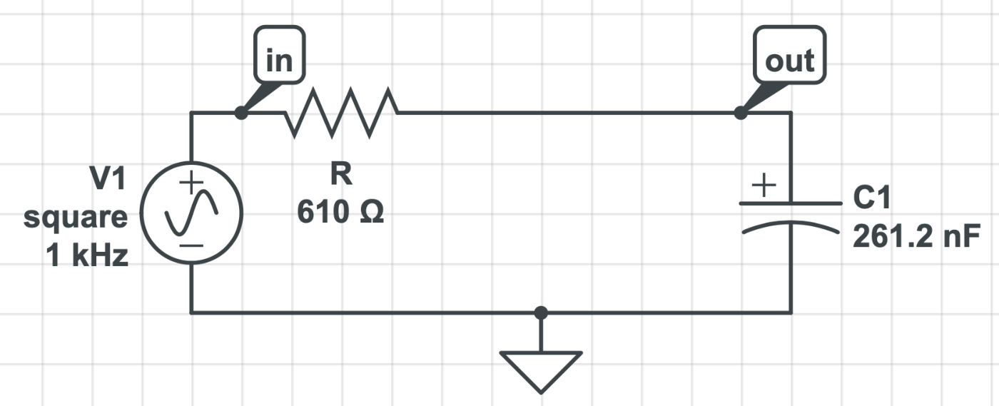
We perform fine-tuning through an NN with a hidden layer consisting of 100 neurons converted into an MILP. The NN inputs are component values (resistor and capacitor) derived from a feasible solution to the MILP or a random sample if a feasible solution does not exist. The continuous design space is for resistor and for capacitor. Since this is a simple design, through prior knowledge, we know that a low-pass filter can be synthesized within these ranges of component values to meet the specifications. The targeted outputs of the NN are gain, bandwidth, and response of the filter at 200, 500, and 2000 Hz. The responses at these frequencies sufficiently capture the behavior of the filter below and above the desired bandwidth. The output constraints are as follows: gain (from input to output) in the range dB and bandwidth in the range Hz. We generate 10 random input samples to initialize the NN for training to minimize the MSE. The solutions suggested by MILP meet the requirements after 20 more simulations. We show these simulations (10 for initialization of the NN and 20 during the MILP step) in Fig. 8: initialization points in the orange part and MILP ones in the blue part. The outcomes during initialization are random as they are far from meeting the requirements. However, the points suggested by the MILP have a response closer to the requirements until finally, the suggested point meets the specification. Fig. 9 shows the component values on termination of Step 2.

V Synthesis Methodology
In this section, we describe ASSENT in detail. The first step explores a large design space using GA. The outcome of the first step is a coarse design that is fine-tuned in Step 2 using a sample-efficient search to obtain component values that satisfy all the constraints and try to improve the value of the objective function attained in Step 1.
V-A Step 1: Coarse design
Design of systems with multiple choices for architectures and component values requires search in a large design space. We achieve this through GA mainly due to its ease of encoding architectures and component values. GA also helps in exploring the entire design space, thus avoiding local minima. We discretize the large design space to obtain a coarse design. The coarse design may even violate hard constraints or attain an inferior value of the objective function compared to other synthesis methodologies.
We show the flow involved in the synthesis of the coarse design in Fig. 10. We evolve individuals across generations using NSGA-II [16] that yields nondominated solutions of the system design formulated as an MOO problem. In architecture search, we initialize some individuals in the first GA generation with seed design(s) from the literature to exploit prior knowledge. When performing only component selection, we initialize the individuals in the first generation with component values to cover the design space. This enables comparisons with other designs from the literature that do not use prior knowledge.

During architecture search, a gene has three constituents: type of component, nodes connecting the component, and the component value, as shown in Fig. 5. In the case of component selection, the gene encodes the value of the component in the chromosome that represents the circuit.
Algorithm 1 describes architecture search using GA. We generate P individuals in a generation. Some of these are from seed designs (S) and others randomly generated. We generate random individuals by selecting a random component, choosing the number of nodes (e.g., a resistor requires two nodes whereas a MOSFET requires three nodes) connected to that component, and the component value. We select the component values for random individuals from quasi-random Sobol samples in the range (R) of each component. Sobol samples are distributed uniformly over a unit hypercube [29]. Then we scale the samples to lie within the specified range for each component. We post-process individuals to ensure that some components connect to the fixed terminals of the architecture, e.g., ground, supply voltage, input/output terminals in the case of a circuit, to ensure a valid design. We simulate all individuals in a generation to compute the objective functions. If the simulation is expensive, we utilize multiple cores and run GA in parallel. We store all the simulations in a buffer B to be used in Step 2, if necessary. We also use the buffer as a lookup table in case the same design needs to be simulated again in Step 1. Next, we rank the individuals using the NSGA-II algorithm [16]. We use tournament selection for selecting some individuals in a generation to undergo reproduction through crossover with a probability of cross and mutation with a probability of mut to produce P children. We use NSGA-II again to select P individuals out of the 2P individuals for the next generation. This process continues until one of the stopping criteria (stop) is met. These criteria are based on individuals not improving over a fixed number of generations, exhausting the simulation budget, or on attaining the required performance. Finally, we select one individual from the final generation based on a performance metric. The metric (lower the better) in our case is one of the multiple objectives or constraints. We select an individual from the last generation since ranking using NSGA-II ensures that we never lose an individual from the Pareto front within a generation. We select only one individual since GA only synthesizes a coarse system design, although it is also possible to select another individual to undergo fine-tuning in the next step.
Component selection for a fixed architecture uses a setup similar to Algorithm 1. Instead of initializing some individuals in the first generation by seed designs, we initialize all the individuals using Sobol samples. The rest of the procedure remains the same.
V-B Step 2: Fine-tuning
The design obtained from Step 1 may not always meet the hard constraints. Even if it meets the hard constraints, it is possible to improve the value of the objective function by searching in a continuous design space. When using Step 1 for architecture search, we use human intervention to refine the synthesized design if needed. We fine-tune this design through a modified version of CNMA [4] by searching in a continuous space. In contrast to CNMA where the component selection stops on exhausting the simulation budget, we adaptively replace the design from Step 1 to improve the value of the objective function. Fig. 11 shows a high-level overview of this step through an example. The designer specifies the system requirements shown on the right in green. The feasible solution of the MILP determines the potential component values shown on the left in blue that achieve the desired response.

Fig. 12 shows the procedure to fine-tune the design that Step 1 yields. In the flowchart, N denotes the number of simulations in a particular trial out of a total of T trials. We effectively repeat the fine-tuning step T times, allowing a maximum of N valid simulations in a trial. We consider a simulation to be invalid if the output from the simulator yields an error. We represent the best value of the objective attained from Step 1 by best_obj. Next, we generate Sobol samples from the range of each component in the design from Step 1, followed by simulation of these points to determine their outputs. We generate samples around the nominal values of each component (e.g., of 10 for resistor). We clip the samples to ensure that the component values are within the permissible range. We model the response of the system to the inputs using an NN. We either pre-train the NN using the simulations saved from Step 1 and the Sobol samples or only on the Sobol samples generated around the best design determined from Step 1. We use the simulations saved from Step 1 to attain better value of the objective function in fewer samples. However, this is not suitable for some systems where the number of samples required may be higher to overcome the inductive bias since Step 1 searches over the entire design space. We select the best NN from an NN architecture library that yields the least MSE on the validation set. We update the NN architecture after every U valid simulations. We convert the NN into an MILP using Eq. (2) to see if there is a feasible solution. We determine the constraints from the desired output of the system. The range of available components determines the constraints on the input. We use Gurobi [30] to find a feasible solution to the MILP problem. If such a solution exists, it indicates that the desired output is reachable by the NN from this input. We simulate the system with the suggested input. If the simulation is invalid, we use Sobol samples until attaining a valid simulation output. We update best_obj when the value of the objective function improves. We then add the input-output pair corresponding to the feasible solution to the training set. If the solution to the MILP problem is infeasible, we generate a Sobol sample and add the corresponding output to the training set. The procedure continues until a maximum number of permissible simulations (N) is exhausted.

After finishing a trial, the input corresponding to the least absolute sum in terms of fractional deviation of the output from the requirement replaces the design from Step 1. Fractional deviation is computed as follows:
| (4) |
where is the specification for the objective or constraint, is the observed response of the system for the objective or constraint. is an indicator function that takes the value 1 in the case of violation of determined by (can be greater or less than) and 0 otherwise. After the last trial, we return the input that corresponds to the output that satisfies all the hard constraints and yields the best value of the objective function.
VI Experimental Results
In this section, we first illustrate how ASSENT can be used for component selection in the design of the following benchmarks: Lunar lander [5], Acrobot [5], Polak3 [6], Waveglider [7], Rover path planning [8], and sensor placement for a power grid [9]. Then we show how ASSENT can be used to synthesize electrical circuits in two cases. In the first case, we use ASSENT for architecture search and component selection to design a circuit that achieves the functionality of a two-stage transimpedance amplifier. In the second case, we select the component values for a fixed architecture for two-stage and three-stage transimpedance amplifiers. We implement ASSENT using Keras [31], Scikit-learn [32], Gurobi [30], and PyGMO [33]. The simulations are performed on an Intel Xeon processor with 64 GB of DRAM.
VI-A Component selection for system design
We illustrate the selection of component values on various benchmarks and compare their performance to that of designs obtained using CNMA [4] with 1, 5, and 10 solvers.
Lunar lander: The goal is to maximize the reward obtained by the landing position subject to constraints on the fuel used and the time taken to land. We run Step 1, i.e., GA for component selection with 100 individuals for a maximum of 400 generations. We set the crossover probability (cross) to 0.9 and mutation rate (mut) to 0.1 that are typical values for GA. We terminate Step 1 if any of the following stopping criteria are met: (1) reward is above 500, (2) after the generation, the objective value for reward does not improve for 10 generations, or (3) we reach the maximum number of generations. We convert the constraints into objectives in Step 1 and formulate the problem as an MOO. There are three objectives in Step 1 described next.
- •
Objective for fuel consumption:
(5) where is set to 15 and represents the penalty for fuel consumption () when it exceeds the maximum permissible value (), which is 100 units in our case. is an indicator function that takes a value of 1 when , and otherwise.
- •
Objective for time taken to land is defined in the same way as fuel consumption. The maximum time allowed for landing is 10 units.
- •
Objective for reward is defined as:
(6) where is the reward for a particular choice of component values. As we need to maximize the reward, the lower the value of Eq. (6), the better is the design. The first term in Eq. (6) yields lower value of the objective for a higher reward. We choose 400 as the numerator since it is close to the reward attained using sequential CNMA (437.1). The second term corresponds to the case for negative reward. We set this term to a large number to penalize designs with a negative reward.
In case of simulation that does not lead to success, we set the objective values to a very large number to indicate this fact.
Table I shows the rewards and constraints for the designs obtained using CNMA and ASSENT. In the table, CNMA-1, CNMA-5, and CNMA-10 refer to CNMA runs based on 1, 5, and 10 solvers, respectively [4]. Step 1 requires less time compared to CNMA, since GA does not need to solve the time-consuming MILP formulation after simulation.
| Procedure | # Simulations | Total time | # Initial samples | fuel 75 | time 10 | reward |
|---|---|---|---|---|---|---|
| CNMA-1 | 2,066 | 1,500s | 100 | 34.12 | 2.60 | 437.1 |
| CNMA-5 | 1,358 | 1,500s | 100 | 59.91 | 2.88 | 469.6 |
| CNMA-10 | 1,494 | 1,500s | 100 | 43.35 | 3.92 | 465.1 |
| Step 1 | 1,400 | 42s | - | 52.59 | 2.64 | 451.4 |
| Step 2 | 583 | 54,000s | 1 | 47.09 | 3.50 | 475.7 |
In Step 2, we aim to improve the reward further. We set the number of trials () to 50, maximum number of iterations () to 20 in the first trial, and 50 from the second trial onwards. We terminate Step 2 at the end of 15 hours. We use all the simulations saved from Step 1 with a reward greater than 400 to narrow down to a promising part of the design space. We generate Sobol samples within % of the design attained in Step 1. Since we use the simulation results from Step 1, we generate only one additional Sobol sample in each trial. We set the update frequency () of the NN architecture search to 10. We select an NN with one of the following architectures (A): [(40,20,8), (30), (15), (100), (50), (200), (20,20,8), (300), (400), (500), (600)], where the tuples represent the number of neurons in the hidden layer(s). The NN inputs represent component values and the outputs represent fuel consumption, time taken to land, and reward. We use a Multi-Layer Perceptron Regressor from the Scikit-learn [32] package along with the Adam optimizer [34], an initial learning rate of 0.0001, adaptive learning, and a maximum iteration count of 100,000 to train the NN. We set other parameters to their default values. Unless otherwise specified, we use the same setup for all the experiments.
The last row of Table I shows the reward attained after fine-tuning. Step 2 requires more time than taken by CNMA, primarily due to the time required for NN architecture search and due to the different system configurations used to run the experiments. We improve the value of the reward from 451.4 to 475.7. Fig. 13 plots the highest reward attained versus the number of simulations. To the left of the dotted line is the reward attained in Step 1 and to the right the reward attained in Step 2. We observe that fine-tuning helps further improve the reward.

Acrobot: The objective is to minimize the time required to stabilize () the system by selecting the design parameters for the two arms of the Acrobot. We terminate GA if falls below 3.2s. Other stopping criteria are the same as the ones used in the Lunar lander example. Table II shows a comparison of attained using CNMA and ASSENT. Step 1 yields a design with s.
| Procedure | # Simulations | Total time | # Initial samples | (s) |
|---|---|---|---|---|
| CNMA-1 | 247 | 1.4 hrs | 20 | 3.4 |
| CNMA-5 | 285 | 1.4 hrs | 20 | 3.2 |
| CNMA-10 | 520 | 1.4 hrs | 20 | 2.8 |
| Step 1 | 1,386 | 2.8 hrs | - | 3.0 |
| Step 2 | 1,359 | 15 hrs | 1 | 2.6 |
| Step 2- tight bound | 1,293 | 15 hrs | 1 | 2.4 |
In Step 2, we fine-tune the component values to further reduce . We use all the simulations saved in Step 1 with s. We select an NN with one of the following architectures (A): [(10), (15), (20), (30), (100)]. We reduce the value of to 2.6s. We further explore if tightening the bounds within which we generate the inputs to % from % of the nominal design from Step 1 can reduce . These results are shown in the last row of Table II. The modified setup yields a design with equal to 2.4s. Fig. 14 plots the best value of versus the number of simulations.

Waveglider: The objective in this benchmark is to maximize subject to the constraints . Here, () is the force of the boat (glider) and () is the velocity of the boat in the () direction. The component values represent the dimensions of the boat and hydrofoil. We define the following objectives for GA:
- •
Objective corresponding to the deviation between and :
(7) where , and .
- •
Objective corresponding to :
(8) where .
- •
The third objective is . We reverse the sign as we need to maximize the velocity of the boat in the direction.
| Procedure | # Simulations | Total time | # Initial samples | |||
|---|---|---|---|---|---|---|
| CNMA-1 | 1,920 | 0.69 hr | 30 | 3.90 | 2.286 | 107.53 |
| CNMA-5 | 3,170 | 0.69 hr | 30 | 3.90 | 2.286 | 107.48 |
| CNMA-10 | 3,920 | 0.69 hr | 30 | 3.90 | 2.286 | 107.48 |
| Step 1 | 2,145 | 0.37 hr | - | 3.61 | 2.286 | 248.83 |
| Step 2 | 2,383 | 15 hrs | 1 | 3.90 | 2.286 | 108.95 |
Table III shows the value of obtained using CNMA and ASSENT. Step 1 terminates after 2,145 simulations in 0.37 hr due to saturation in performance.
In Step 2, we use all the valid simulations from Step 1 to train the NN. We select an NN with one of the following architectures (A): [(10), (15), (20), (30), (100)]. Besides the three outputs from the simulator, we add an additional output when training the NN. This output is an identity mapping of . It simplifies the MILP formulation by transferring the constraints to the NN output. We do not range-normalize the outputs to keep and to the same scale. We also increase the learning rate to 0.1 to speed up training. The design synthesized at the end of Step 2 meets all the constraints and improves the value of to 3.90 m/s. Fig. 15 plots the best value of vs. number of simulations.

Polak3: The objective is to minimize the maximum value of 10 different transcedental functions. There are 11 inputs that represent component values. The objective of GA is to find the maximum value of the transcedental functions.
| Procedure | # Simulations | Total time | # Initial samples | Objective |
|---|---|---|---|---|
| CNMA-1 | 859 | 2,000s | 20 | 5.97 |
| CNMA-5 | 1,970 | 2,000s | 20 | 6.06 |
| CNMA-10 | 2,700 | 2,000s | 20 | 5.98 |
| Step 1 | 37,397 | 72s | - | 5.94 |
As simulations are not time-consuming for this problem, we let GA run serially for 400 generations. Step 1 requires a total of 37,397 simulations in 72s, as shown in Table IV. We attain an objective value of 5.94 compared to 5.97 obtained using CNMA. Our solution is closer to the known minimum value of 5.93 for this problem. Fine-tuning using Step 2 does not improve the value of this objective. This indicates that if the simulations are cheap, Step 1 may alone be sufficient to solve the optimization problem without the need of fine-tuning in Step 2. Fig. 16 plots the value of the objective function vs. number of simulations.

Rover path planning: The objective is to find a trajectory that minimizes a cost function by selecting 30 2D points that define the trajectory. We use this cost function as the objective for GA. We let GA run for 400 generations since the simulations are not time-consuming. Step 1 requires a total of 40,000 simulations in 188s, as shown in Table V. We obtain an objective value of 0.369 compared to 0.778 obtained using CNMA. Fine-tuning using Step 2 does not improve the value of this objective further. Fig. 17 plots the best value of the objective versus the number of simulations.
| Procedure | # Simulations | Total time | # Initial samples | Cost |
| CNMA-1 | 1,848 | 9,000s | 2 | 1.148 |
| CNMA-5 | 2,639 | 9,000s | 2 | 0.997 |
| CNMA-10 | 4,454 | 9,000s | 2 | 0.778 |
| Step 1 | 40,000 | 201s | - | 0.369 |

IEEE 118 bus Sensor placement: The objective is to obtain the sensor placement such that sensor readings give the best chance of predicting the line failure pattern. The failure pattern is determined by the “ambiguity” in the sensor pattern. The maximum number of sensors is 50. We define the following two objectives for GA:
- •
The first objective is to capture the constraint on the number of sensors:
(9) where denotes the number of sensors used in a particular configuration. We apply a penalty of when using more than 50 sensors.
- •
The second objective is to minimize ambiguity as determined by the simulator output.
Step 1 terminates after 1,500 simulations due to saturation in performance for 10 generations. Table VI shows that Step 1 achieves an ambiguity of 0.0107 in 1,500 simulations. The ambiguity is lower by about 50 than the ambiguity attained using CNMA. Fig. 18 plots the value of ambiguity vs. the number of simulations.
| Procedure | # Simulations | Total time | # Initial samples | Ambiguity |
| CNMA-1 | 251 | 1,500s | 30 | 0.04813 |
| CNMA-5 | 490 | 1,500s | 30 | 0.02139 |
| CNMA-10 | 380 | 1,500s | 30 | 0.02139 |
| Step 1 | 1,500 | 1,058s | - | 0.01070 |

VI-B Circuit design
In this section, we evaluate how ASSENT performs architecture search and component selection for electrical circuits. We compare our results with those in [10] that are synthesized by humans, RL, and Bayesian optimization. The technology files that specify the device physics for simulation are from [35] and are the same as in [10].
VI-B1 Architecture search and component selection
We use the standard design of a two-stage transimpedance amplifier presented in [10] as the seed design for our methodology to take advantage of prior human knowledge. Fig. 19 shows this seed design. The objectives are to maximize the amplifier’s bandwidth and minimize the sum of MOSFET gate areas in the circuit while satisfying hard constraints on noise, gain, peaking, and power. The design space comprises three components: two types of MOSFETs (PMOS, NMOS) and resistor. In the human-designed circuit, the MOSFETs are of minimum length (), based on the technology used, whereas the width is variable. Our search also uses minimum-length MOSFETs and only selects their width. We discretize the design space during architecture search (Step 1) by generating 100 Sobol samples for resistors in the range and width in the range. In the human-designed circuit, the resistor values are and , and the width is in the range. During GA evolution, we allow the circuit to have a maximum of 11 nodes and a total of 10 components, whereas the seed design has six nodes and eight components, to enable search for novel designs. Since we need to represent 10 components in a chromosome, we initialize two additional genes as resistors with a small resistance of 2.2 whose terminals are shorted and not connected to any of the nodes in the seed design. This ensures the response of the seed design remains unaffected.

We use GA to evolve a generation of 100 individuals and set the maximum number of generations to 200. We choose these numbers to achieve at least about sample efficiency (i.e., fewer simulations) compared to the design methodology in [10]. We simultaneously search for the architecture and the component values, whereas the method in [10] only searches for component values. Hence, our method searches through a much larger design space, albeit with the seed design. We formulate an MOO problem with three objectives: bandwidth, noise, and power. The objectives are described next.
- 1.
Bandwidth: This objective corresponds to the weighted sum of the absolute difference between the desired and observed responses, with a passband weight of 40 and a stopband weight of 1. We use the following reward/penalty. (a) Assessing the level of reward/penalty is based on the operating region of each MOSFET: reward for MOSFET operating in the saturation region, else a penalty. We use a reward of 1 for operation in the saturation region. We apply a penalty of 2 (3) for operation in the linear (cutoff) region. We sum the rewards and penalty for each MOSFET and divide by the number of MOSFETs. (b) A penalty of 15 is assessed based on the fractional deviation in gain below 58.1 dB (since 58.1 dB is the gain achieved by RL based synthesis in [10]). (c) A penalty of 15 is assessed based on the fractional deviation in peaking above 0.963 (achieved by RL in [10]). (d) A penalty of 15 is assessed based on the fractional deviation in bandwidth below 5.81 GHz (this is slightly higher than the bandwidth achieved by RL in [10]: 5.78 GHz). We scale the bandwidth objective by dividing it by the objective of the seed design.
- 2.
Noise: This objective corresponds to the ratio of measured noise and the noise achieved by the RL-based design in [10] (19.2 ). An additional penalty of 15 is assessed based on the fractional deviation in noise above this value.
- 3.
Power: This objective corresponds to the ratio of measured power and the power achieved by the RL-based design in [10] (3.18 ). No penalty is assessed in this case due to the large room for optimization available for power consumption.
The objective for noise is given by
| (10) |
where is the noise of RL-designed circuit, is the measured noise, and = 15 is the penalty. Other objectives are defined analogously.
We club together all the sub-objectives related to bandwidth (gain, desired bandwidth, peaking) into one to minimize the number of objectives that need to be tackled while capturing the entire frequency response. The penalty terms encourage the target response to be better than the response of the designs in [10]. In case the simulation is unsuccessful, we set the objective values to a very large number to indicate this fact.
We use a tournament size of 10, mutation rate of 0.1, and crossover probability of 0.9, same as before. The evolution stops when one the following criteria are met. (1) The scaled bandwidth objective falls below 0.9 since the aim is to improve it by about relative to that of the seed design. (2) The number of generations exceeds 100 and the bandwidth objective stays the same for more than 100 generations, indicating saturation in GA performance. (3) The maximum number of generations (200) is reached.

We choose the circuit with the best value of the objective for bandwidth as the coarse design in Step 1 since this circuit addresses several sub-objectives. We fine-tune the coarse design to meet the specifications in the next step. We remove dangling nodes through human intervention as they are redundant. We also remove a MOSFET operating in the cutoff region as it does not contribute to gain. Fig. 20 shows the circuit before and after human intervention. Table VII shows the values of objectives and constraints before and after human intervention. The row named ASSENT Step 1 shows the results before human intervention. GA requires less than an hour for synthesis. The second last row shows the results after human intervention. After the human intervention, the circuit does not meet the hard constraint for peaking. We remedy the constraint violation in Step 2. The seed design has six MOSFETs. This one uses only four MOSFETs.
In Step 2, we fine-tune the component values to maximize the bandwidth while satisfying all the hard constraints. We use a slightly modified setup for Step 2 than in Section VI-A. Rather than using all the simulations saved from Step 1, we initialize the NN using only Sobol samples around the design from Step 1. We use 20 Sobol samples for initialization in the first trial and 1 Sobol sample in each subsequent trial. We empirically found that using the simulations saved from Step 1 yields inferior results. We attribute this to the inductive bias imposed in Step 1 due to sampling over the entire design space. Sobol samples around the design synthesized in Step 1 enable focus on the region of interest. In all the experiments on electrical circuits, we select an NN with one of the following architectures (A): [(10), (40,20,8), (50)]. We let Step 2 run until 50 trials are over with the other setup being the same, as described in the previous section.
| #Samples | Time | Noise () | Gain () | Peaking () | Power () | Gate area () | Bandwidth () | |
|---|---|---|---|---|---|---|---|---|
| Spec. | - | - | - | maximize | ||||
| Human Design [10] | 1,289,618 | months | 18.6 | 57.7 | 0.927 | 8.11 | 23.11 | 5.95 |
| DDPG [10] | 50,000 | 30 GPU hrs | 19.2 | 58.1 | 0.963 | 3.18 | - | 5.78 |
| Bayesian Opt.[10] | 880 | 30 hrs | 58.6 | 0.629 | 4.24 | - | 5.16 | |
| ASSENT Step 1 | 1,600 | 0.15 hr | 18.0 | 58.0 | 0.913 | 7.97 | 35.59 | 5.93 |
| ASSENT Step 1+Human | - | - | 17.9 | 58.0 | 7.97 | 22.76 | 5.96 | |
| ASSENT Step 1+2 | 4239 | 25.4 hrs | 19.3 | 57.6 | 0.974 | 6.74 | 20.24 | 6.18 |
Table VII 22 2 Gate area is shown only for designs for which this information is available. There was a problem in area calculation in [10] that was confirmed after contacting the authors. shows a comparison of the design synthesized by ASSENT with designs obtained by humans, DDPG, and BO [10]. The last row depicts a design that satisfies all the hard constraints while maximizing bandwidth. We set the required area to less than of the human design when maximizing bandwidth. ASSENT synthesizes a design with a bandwidth of 6.18 GHz in 4,239 simulations. It is about 12 more sample-efficient than DDPG and achieves a much higher bandwidth. ASSENT requires a total of 25.4 CPU hours, whereas DDPG requires 30 GPU (type not specified) hours [10]. Fig. 21 plots the best value of bandwidth vs. the number of simulations. We only plot the results for Step 2 to show component selection results for a fixed architecture.

VI-B2 Component selection for fixed architectures
In this section, we use ASSENT to select component values for fixed architectures of a two-stage and three-stage transimpedance amplifiers.
Two-stage transimpedance amplifier: We use ASSENT to determine the width of all the MOSFETs and resistors with the goal of minimizing the objective functions defined in Section VI-B1. We discretize the design space in Step 1 by generating 100 Sobol samples for resistors in the range and width in the range. These value ranges include those for the human-designed circuit. Table VIII shows a chromosome for this case where corresponds to the width of MOSFET , and and denote the resistors in Fig. 19.
| () | () | () | () | () | () | () | () |
|---|---|---|---|---|---|---|---|
| 0.39 | 47.86 | 0.59 | 24.71 | 15.18 | 7.40 | 750.8 | 2798.8 |
We evolve a generation of 30 individuals for a maximum of 400 generations. We use a smaller population size than in architecture search because the problem is more straightforward due to a smaller design space. The stopping criteria are as follows. (1) The scaled bandwidth with respect to the human design falls below . (2) The number of generations exceeds 100 and bandwidth stays the same for more than 100 generations, indicating saturation. (3) The maximum number of generations, i.e., 400, is reached.
The second last row of Table IX shows the value of the objective function obtained after Step 1. The bandwidth is inferior to that obtained in human design. Hence, in Step 2, we fine-tune the Step 1 design through component selection to improve its performance. The last row of Table IX shows the design synthesized using ASSENT. ASSENT is more than 6 sample-efficient than DDPG and achieves the highest bandwidth among all considered designs. Fig. 22 plots the best bandwidth value vs. the number of simulations used in Step 2.
| #Samples | Time | Noise () | Gain () | Peaking () | Power () | Gate area () | Bandwidth () | |
|---|---|---|---|---|---|---|---|---|
| Spec | - | - | maximize | |||||
| Human Design [10] | 1,289,618 | months | 18.6 | 57.7 | 0.927 | 8.11 | 23.11 | 5.95 |
| DDPG [10] | 50,000 | 30 GPU hrs | 19.2 | 58.1 | 0.963 | 3.18 | - | 5.78 |
| Bayesian Opt. [10] | 880 | 30 hrs | 58.6 | 0.629 | 4.24 | - | 5.16 | |
| ASSENT Step 1 | 5,214 | 0.7 hr | 19.2 | 58.5 | 0.645 | 5.51 | 17.86 | 5.71 |
| ASSENT (Step 1+2) | 7,853 | 77 hrs | 19.2 | 57.6 | 0.949 | 5.60 | 18.15 | 6.12 |

Three-stage transimpedance amplifier: We select the component values for the three-stage transimpedance amplifier shown in Fig. 23, which is adapted from [10]. The blue and green dotted boxes contain subcircuits that are mirror images of each other. Hence, we obtain the component values for only one subcircuit and mirror them in the other. We determine the width and length of all the MOSFETs, including the bias transistor T1. There are 19 components in all: width/length of nine MOSFETs and a resistor Rb.

The objective is to minimize the sum of the gate areas of all the MOSFETs while meeting hard constraints for gain, bandwidth, and power. We discretize the design space during component selection in Step 1 by generating 100 Sobol samples with width in the , length in the , and resistor in the range. The human-synthesized circuit has width in the range, length in the range, and a resistor of . We reduce the design space for width by around to encourage Step 1 to obtain designs with a smaller area. We also round the length to the nearest units since the technology only permits the length to be an integer multiple of . We use this rounding in Step 2 as well.
We have the following objectives:
- 1.
Bandwidth: We set the passband to with a target gain of (this corresponds to a gain of for the half-circuit whereas the minimum gain required for its valid design is or differential gain). We use the following rewards/penalties. (a) A reward for a MOSFET operating in the saturation region, else a penalty is applied. We use a reward of 1 for operation in the saturation region. We apply a penalty of 5 (7) for operation in the linear (cutoff) region. Since the number of MOSFETs is larger than in the earlier design, we slightly increase these numbers to encourage MOSFET operation in the saturation region. (b) Penalty of 15 based on fractional deviation in gain below 80 dB () for the half circuit in Fig. 23. (c) Penalty of 15 based on fractional deviation in bandwidth below .
- 2.
Area: We define the area objective as the ratio of the sum of the areas of the MOSFET in one of the mirrored regions and the area of the bias MOSFET (T1) and the corresponding sum of areas in the human-synthesized circuit.
- 3.
Power: We define this objective as the ratio between measured power and the power consumed by the human-designed circuit, which is . We levy a penalty of 15 based on the fractional deviation in power above this value.
The second last row of Table X shows results of the circuit synthesized using Step 1. This circuit violates the hard constraint on power and is hence not an acceptable design. The area of this circuit is also much higher than that of the human-designed circuit. Hence, in the next step, we fine-tune the component values to minimize the area while satisfying all the hard constraints. The last row of Table X shows the results obtained by ASSENT. We set the initial requirement for the area to . ASSENT synthesizes a design which satisfies all the hard constraints with an area that is around lower than the design obtained using DDPG. ASSENT is around more sample-efficient than DDPG. Fig. 24 plots the best area value vs. the number of simulations. The area is computed after rounding MOSFET length to the nearest 0.2 m.
| #Samples | Time | Bandwidth () | Gain () | Power () | Gate area () | |
| Spec | - | - | - | |||
| Human Design [10] | 10,000,000 | months | 90.1 | 20.2 | 1.37 | 211.0 |
| DDPG [10] | 40,000 | 40 GPU hrs | 92.5 | 20.7 | 2.50 | 90.0 |
| Bayesian Opt. [10] | 1,160 | 40 hrs | 21.1 | 130.0 | ||
| ASSENT Step 1 | 3,060 | 0.5 hr | 90.2 | 22.9 | 337.0 | |
| ASSENT (Step 1+2) | 5,749 | 84.7 hrs | 90.5 | 20.1 | 3.00 | 69.2 |

VII Conclusion
In this article, we formulated nonlinear system design as an MOO problem and proposed a framework called ASSENT to solve it. We used gradient-free search through GA for exploration and CNMA for sample efficiency. CNMA achieves sample efficiency by connecting neural networks with MILP solvers in a new learning-from-failure feedback loop. The methodology provides a flexible framework for discovering efficient architectures and component values or simply the component values for a fixed architecture. Using this framework, we achieve the same or improve the value of the objective functions compared to designs synthesized using CNMA by up to 53. We also synthesized electrical circuits with the best value of the objective function while improving sampling efficiency by 6-12. As part of future work, we plan to formulate nonlinear system design as graph problems in order to explore different architectures by manipulating these graphs and other sample-efficient techniques for active learning. We also plan to enhance the efficacy of the methodology by combining it with RL.
Acknowledgment: We would like to thank Hanrui Wang for providing details of his work and the simulation environment used in [10]. The authors would also like to acknowledge the help provided by Sanjai Narain, Emily Mak, and Karthik Narayan with CNMA and various benchmarks used for evaluation of ASSENT. The simulations presented in this article were performed on computational resources managed and supported by Princeton Research Computing at Princeton University.
References
- [1] K. Sampigethaya and R. Poovendran, “Aviation cyber–physical systems: Foundations for future aircraft and air transport,” Proceedings of the IEEE, vol. 101, no. 8, pp. 1834–1855, 2013.
- [2] A. O. Akmandor and N. K. Jha, “Keep the stress away with SoDA: Stress detection and alleviation system,” IEEE Trans. Multi-Scale Computing Systems, vol. 3, no. 4, pp. 269–282, 2017.
- [3] Z. Zhou, Y. S. Ong, P. B. Nair, A. J. Keane, and K. Y. Lum, “Combining global and local surrogate models to accelerate evolutionary optimization,” IEEE Transactions on Systems, Man, and Cybernetics, Part C (Applications and Reviews), vol. 37, no. 1, pp. 66–76, 2007.
- [4] S. Narain, E. Mak, D. Chee, T. Huster, J. Cohen, K. Pochiraju, B. Englot, N. K. Jha, and K. Narayan, “Fast design space exploration of nonlinear systems: Part I,” under review at IEEE Trans. on Computer-Aided Design, 2021.
- [5] G. Brockman, V. Cheung, L. Pettersson, J. Schneider, J. Schulman, J. Tang, and W. Zaremba, “OpenAI Gym,” 2016.
- [6] E. Polak, D. Q. Mayne, and J. E. Higgins, “A superlinearly convergent algorithm for min-max problems,” in Proc. IEEE Conf. Decision and Control, 1989, pp. 894–898 vol.1.
- [7] N. D. Kraus, “Wave glider dynamic modeling, parameter identification and simulation,” Ph.D. dissertation, Honolulu, Univ. of Hawaii at Manoa, May 2012.
- [8] Z. Wang, C. Gehring, P. Kohli, and S. Jegelka, “Batched large-scale Bayesian optimization in high-dimensional spaces,” in Proc. Int. Conf. Artificial Intelligence and Statistics, 2018, pp. 745–754.
- [9] “OpenDSS, electrical power system simulation tool.” [Online]. Available: https://smartgrid.epri.com/SimulationTool.aspx
- [10] H. Wang, J. Yang, H.-S. Lee, and S. Han, “Learning to design circuits,” arXiv preprint arXiv:1812.02734, 2018.
- [11] W. Lyu, F. Yang, C. Yan, D. Zhou, and X. Zeng, “Batch Bayesian optimization via multi-objective acquisition ensemble for automated analog circuit design,” in Proc. Int. Conf. Machine Learning, 2018, pp. 3306–3314.
- [12] W. B. Powell, “A unified framework for stochastic optimization,” European J. Operational Research, vol. 275, no. 3, pp. 795–821, 2019.
- [13] V. Mnih, K. Kavukcuoglu, D. Silver, A. Graves, I. Antonoglou, D. Wierstra, and M. Riedmiller, “Playing Atari with deep reinforcement learning,” in Proc. NIPS Deep Learning Workshop, 2013.
- [14] T. P. Lillicrap, J. J. Hunt, A. Pritzel, N. Heess, T. Erez, Y. Tassa, D. Silver, and D. Wierstra, “Continuous control with deep reinforcement learning,” in Proc. Int. Conf. Learning Representations, 2016.
- [15] R. S. Zebulum, M. A. Pacheco, and M. M. B. Vellasco, Evolutionary Electronics: Automatic Design of Electronic Circuits and Systems by Genetic Algorithms. CRC press, 2018.
- [16] K. Deb, A. Pratap, S. Agarwal, and T. Meyarivan, “A fast and elitist multiobjective genetic algorithm: NSGA-II,” IEEE Trans. Evolutionary Computation, vol. 6, no. 2, pp. 182–197, 2002.
- [17] K. V. Price, An Introduction to Differential Evolution, New Ideas in Optimization. McGraw-Hill Ltd., Maidenhead, UK, 1999.
- [18] M. Dorigo, M. Birattari, and T. Stutzle, “Ant colony optimization,” IEEE Computational Intelligence Magazine, vol. 1, no. 4, pp. 28–39, 2006.
- [19] J. Kennedy and R. Eberhart, “Particle swarm optimization,” in Proc. IEEE Int. Conf. Neural Networks, 1995, pp. 1942–1948.
- [20] J. R. Koza, F. H. Bennett, D. Andre, M. A. Keane, and F. Dunlap, “Automated synthesis of analog electrical circuits by means of genetic programming,” IEEE Trans. Evolutionary Computation, vol. 1, no. 2, pp. 109–128, 1997.
- [21] J. D. Lohn and S. P. Colombano, “A circuit representation technique for automated circuit design,” IEEE Trans. Evolutionary Computation, vol. 3, no. 3, pp. 205–219, 1999.
- [22] G. Nicosia, S. Rinaudo, and E. Sciacca, “An evolutionary algorithm-based approach to robust analog circuit design using constrained multi-objective optimization,” in Proc. Int. Conf. Innovative Techniques and Applications of Artificial Intelligence, 2007, pp. 7–20.
- [23] K. Settaluri, A. Haj-Ali, Q. Huang, K. Hakhamaneshi, and B. Nikolic, “Autockt: Deep reinforcement learning of analog circuit designs,” in Proc. Design, Automation & Test in Europe Conference & Exhibition, 2020, pp. 1–6.
- [24] D. A. Van Veldhuizen and G. B. Lamont, “Evolutionary computation and convergence to a Pareto front,” in Proc. Late-breaking Papers at the Genetic Programming Conference, 1998, pp. 221–228.
- [25] D. E. Goldberg and J. H. Holland, Genetic Algorithms and Machine Learning. Kluwer Academic Publishers-Plenum Publishers, 1988.
- [26] T. Blickle and L. Thiele, “A comparison of selection schemes used in evolutionary algorithms,” Evolutionary Computation, vol. 4, no. 4, pp. 361–394, 1996.
- [27] M. Akintunde, A. Lomuscio, L. Maganti, and E. Pirovano, “Reachability analysis for neural agent-environment systems,” in Proc. Int. Conf. Principles of Knowledge Representation and Reasoning, 2018.
- [28] G. Venturini, “Ahkab 0.18 docs,” 2015. [Online]. Available: https://ahkab.readthedocs.io/en/latest/examples/Python_API.html
- [29] S. Burhenne, D. Jacob, and G. P. Henze, “Sampling based on Sobol sequences for Monte Carlo techniques applied to building simulations,” in Proc. Int. Conf. Build. Simulation, 2011, pp. 1816–1823.
- [30] L. Gurobi Optimization, “Gurobi optimizer reference manual,” 2020. [Online]. Available: http://www.gurobi.com
- [31] F. Chollet et al. (2015) Keras. [Online]. Available: https://github.com/fchollet/keras
- [32] F. Pedregosa, G. Varoquaux, A. Gramfort, V. Michel, B. Thirion, O. Grisel, M. Blondel, P. Prettenhofer, R. Weiss, V. Dubourg, J. Vanderplas, A. Passos, D. Cournapeau, M. Brucher, M. Perrot, and E. Duchesnay, “Scikit-learn: Machine learning in Python,” J. Machine Learning Research, vol. 12, pp. 2825–2830, 2011.
- [33] D. Izzo, “PyGMO and PyKEP: Open source tools for massively parallel optimization in astrodynamics (the case of interplanetary trajectory optimization),” in Proc. Int. Conf. on Astrodynamics Tools and Techniques, 2012.
- [34] J. Duchi, E. Hazan, and Y. Singer, “Adaptive subgradient methods for online learning and stochastic optimization.” J. Machine Learning Research, vol. 12, no. 7, 2011.
- [35] H. Mao, P. Negi, A. Narayan, H. Wang, J. Yang, H. Wang, R. Marcus, R. Addanki, M. Khani Shirkoohi, S. He, V. Nathan, F. Cangialosi, S. Venkatakrishnan, W.-H. Weng, S. Han, T. Kraska, and D. Alizadeh, “Park: An open platform for learning-augmented computer systems,” in Proc. Neural Information Processing Systems, 2019, pp. 2494–2506.