A Latent space solver for PDE generalization

Rishikesh Ranade Chris Hill Haiyang He Amir Maleki & Jay Pathak Affiliation: Ansys Inc Affiliation: Canonsburg, PA 15317, USA Affiliation: {rishikesh.ranade, chris.hill, haiyang.he, amir.maleki & jay.pathak}@ansys.com

Abstract

In this work we propose a hybrid solver to solve partial differential equation (PDE)s in the latent space. The solver uses an iterative inferencing strategy combined with solution initialization to improve generalization of PDE solutions. The solver is tested on an engineering case and the results show that it can generalize well to several PDE conditions.

1 Introduction

Simulations are important in engineering applications to explore the underlying physics. But, they can be computationally expensive because they involve numerical methods to solve partial differential equations (PDEs) for various conditions associated with the PDE, such as geometry of computational domain, type of boundary conditions (BC), external source terms etc. Researchers have explored the idea of coupling machine learning with PDEs for several decades (Crutchfield & McNamara 1987; Kevrekidis et al. 2003). Recently, there is a tremendous focus on improving the predictive capability and generalizability of ML methods by infusing physics, either during training or prediction. A substantial portion of research has focused on introducing physics-based constraints in neural networks through the computation of PDE derivatives (Raissi et al. 2019; Raissi & Karniadakis 2018; Rao et al. 2020; Ranade et al. 2020; Gao et al. 2020; Wu et al. 2018; Qian et al. 2020; Xue et al. 2020). More recently, there is a huge effort on training neural networks within frameworks of differentiable PDE solvers. These approaches use differentiable solvers to learn and control PDE solutions as well as the dynamics of the system (Amos & Kolter 2017; Um et al. 2020; de Avila Belbute-Peres et al. 2018; Toussaint et al. 2018; Wang et al. 2020; Holl et al. 2020; Portwood et al. 2019; Bar-Sinai et al. 2019; Zhuang et al. 2020; Kochkov et al. 2021).

There is a growing need for improving generalizability of ML techniques to a wider range of PDE parameters. The existing ML approaches that learn from PDE conditions, such as geometry, BCs and source terms have to handle several challenges. Firstly, the PDE conditions can be high dimensional and sparse, impacting learning and generalizability. Secondly, the inference procedure is static and there are limited opportunities to alter the trajectory of PDE solutions. Finally, the space of physical solutions is very large.

In this paper, we propose a hybrid solver to learning PDE solutions and address the outlined challenges. We use lower dimensional representations to tackle the issues of high dimensionality and sparsity of PDE conditions and solutions. Further, the inferencing methodology uses an iterative procedure to solve the PDE in a lower dimensional latent space with fixed point iterations. Latent space learning has been explored in several works, (Wiewel et al. 2020; Maulik et al. 2020; Kim et al. 2019; Murata et al. 2020; Fukami et al. 2020b; Champion et al. 2019; Fukami et al. 2020a; He & Pathak 2020), but our approach to solve PDEs is different and novel. The iterative procedure at inference enables us to alter the solution trajectories using existing PDE solvers. This is useful in ML based techniques to ensure solver robustness, generalizability and accuracy. The hybrid solver combines solution initialization using existing coarse grid PDE solvers with this iterative inferencing procedure and is demonstrated on a practical engineering application.

2 Solution Methodology

2.1 Latent space representation

Refer to caption — Figure 1: Autoencoders for PDE conditions and solution

Fig. 1 shows the neural network architectures used to determine the compressed latent space vectors of the various PDE conditions, such as geometry of computational domain, BCs and source term distributions, and PDE solutions ( $u_{1}$ and $u_{2}$ ). The geometry of the computational domain is represented using a binarized level set representation (Osher & Sethian 1988). On the other hand, boundary conditions and source terms already have spatio-temporal distributions. The PDE conditions, as well as the PDE solutions are compressed into their lower dimensional latent vectors, $\eta_{g},\eta_{h},\eta_{b},\eta$ , using CNN encoder-decoder type networks. The loss functions used to constrain the Autoencoder networks of PDE conditions are purely statistical. Conversely, the PDE solution Autoencoders are augmented by including PDE based loss constraints, similar to Ranade et al. 2020. The PDE constraints are computed using the discretization schemes, available in the Ansys suite of software. Additionally, since the PDE solutions are dependent on other PDE conditions, the solution Autoencoders are also conditioned upon the latent vectors of the PDE conditions.

2.2 Hybrid latent space solver methodology

Fig. 2 shows the hybrid latent space solver methodology proposed in this work for using the Autoencoder networks to infer at unknown and unseen conditions. The iterative procedure based on fixed point iterations and is motivated from our previous work, (Ranade et al. 2020). The different steps involved in the solution procedure are outlined below.

1.

Latent vectors, $\eta_{g}$ , $\eta_{h}$ and $\eta_{b}$ , are computed for a new computational domain geometry, boundary condition and source term distribution using the encoder networks.
2.

The initial solution of PDE is computed using an existing PDE solver on a very coarse grid. These solutions are interpolated on the fine grid and encoded to their latent vector form, $\eta$ .
3.

The initial solution latent vector, $\eta$ combined with $\eta_{g}$ , $\eta_{h}$ and $\eta_{b}$ is passed through the decoder to generate solution fields, ${u_{1}},{u_{2}}$ .
4.

Solution fields are compressed to a new solution latent vector, $\hat{\eta}$ , using the the encoder.
5.

Steps $3$ and $4$ are repeated with the new solution latent vector, $\hat{\eta}$ until $||\eta-\hat{\eta}||_{2}<1e^{-6}$ .
6.

At convergence, the PDE solutions are decoded using the most recent $\hat{\eta}$ .

The hybrid latent space solver described above has two main implications. Firstly, the iterative procedure used for inferencing allows initialization of solutions using existing PDE solvers and moreover provides an opportunity to intervene the solution process and alter the solution trajectory using PDE solvers. Secondly, the solution procedure is conditioned by richer, lower dimensional representations of PDE conditions in the form of latent vectors, thus enhancing the generalizability.

3 Results and discussions

The hybrid solver is demonstrated for a 3-D, steady-state electronic cooling case with natural convection. There are $5$ solution variables, $3$ components of velocity, pressure and temperature. The geometry of the computational domain may be observed in Fig. 3. The domain consists of a chip-mold assembly held by a PCB and the entire geometry is placed inside a fluid domain. The chip is subjected to heat sources with random spatial distributions due to uncertainty in electrical heating. Fig. 6 in Appendix A shows an example of the $8$ different distributions of heat sources. From a physics standpoint, natural convection results in a two-way coupling between temperature and velocity. The heat source specified results in a temperature increase, which generates fluid velocity because of buoyancy effects and in turn cools the chip. At steady state there is sufficient velocity generation to cancel out the heat generation. The main challenges in this case are to capture the complicated physics resulting from the two-way coupling and to generalize to different spatial distributions of heat sources.

3.1 Data generation and training

The Autoencoder for heat source distribution is trained with random spatial distributions generated using a Gaussian mixture model, where the number of Gaussians are varied from $1$ to $20$ for randomized mean and variance. The Autoencoder is set up to achieve a compression ratio of around $12$ . The PDE solution Autoencoder is trained with $200$ solution generated using Ansys Fluent fluid flow simulation software on a computational mesh with $128^{3}$ elements for random heat sources. A compression ratio of $64$ is achieved. The normalized reconstruction mean squared error for unseen test samples is to the order of $1e^{-6}$ for all the solution variables as well as the heat source.

3.2 Comparisons with Ansys Fluent

The hybrid solver is compared with Ansys Fluent solution for two heat source distributions, which are generated randomly and thus, never seen by the networks. The initial solution is computed at a mesh resolution of $16$ elements in each spatial direction in Ansys Fluent for 200 steady-state iterations.

3.2.1 Computation time

Ansys Fluent takes an average of $200$ minutes on a single CPU to obtain a converged solution on $128^{3}$ mesh. On the other hand, the hybrid solver converges in $50$ seconds on average, including the time it takes to generate the coarse grid solution. Thus, the hybrid solver results in a 200x speedup over Ansys Fluent in generating solutions on fine girds. The averages are calculated over runs on 100 cases with different heat source distributions.

3.2.2 Contour & Line plots

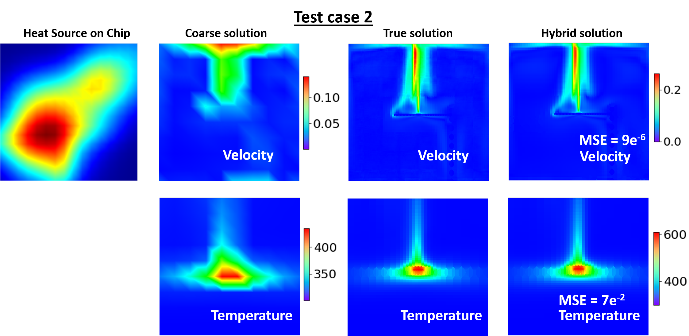
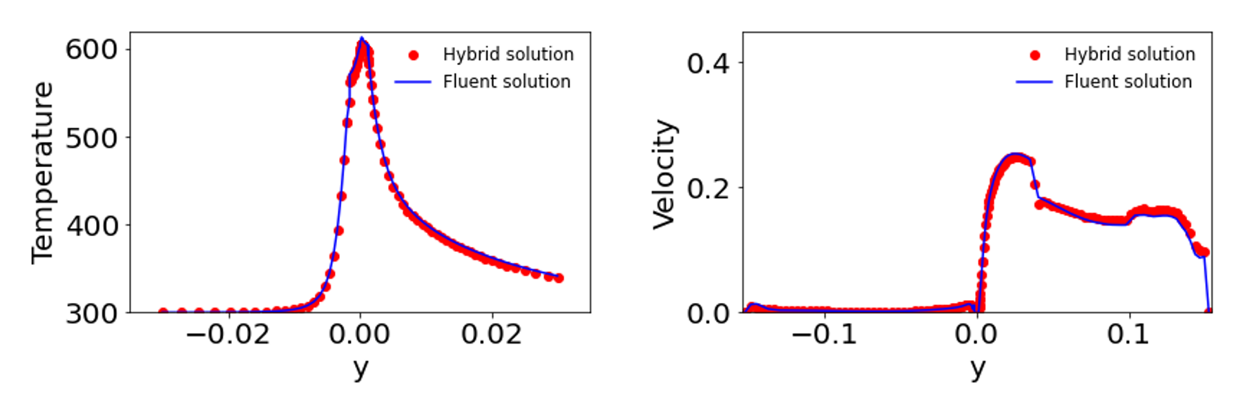
Fig. 4 and Fig. 7 in Appendix A compare the solution contours on the X-Y plane for the two test cases. The hybrid solution agrees well with respect to the Ansys Fluent solutions with small mean squared errors. Although not shown here, the performance is similar for a variety of random distributions of heat source, including the examples shown in Figure 6 in the Appendix A. The line plots in Fig. 5 and Fig. 8 in Appendix A are plotted along the Y direction through chip center. It can be observed that the overall trends as well as the peak quantities agree well for both velocity and temperature in both test cases. The contour and line plots show that the hybrid latent space solver captures the two-way coupled physics accurately and more importantly, the methodology generalizes well to a variety of heat source distributions.

4 Conclusion and Future work

In this work we have proposed a hybrid solver that combines latent space learning with solution initialization to improve generalization of PDE solutions. The results shows that the methodology is computationally fast, accurate and generalizable. In its current form, the proposed methodology has several limitations. Most notably, the approach is restricted to structured domains with fixed resolutions with relatively simpler computational domain geometries. In future, we would like to extend this to solve on unstructured meshes. Furthermore, the latent space iterative strategy will be integrated with an actual PDE solver to alter solution trajectories and improve convergence.

References

Amos & Kolter (2017) Brandon Amos and J Zico Kolter. Optnet: Differentiable optimization as a layer in neural networks. In International Conference on Machine Learning, pp. 136–145. PMLR, 2017.
Bar-Sinai et al. (2019) Yohai Bar-Sinai, Stephan Hoyer, Jason Hickey, and Michael P Brenner. Learning data-driven discretizations for partial differential equations. Proceedings of the National Academy of Sciences, 116(31):15344–15349, 2019.
Champion et al. (2019) Kathleen Champion, Bethany Lusch, J Nathan Kutz, and Steven L Brunton. Data-driven discovery of coordinates and governing equations. Proceedings of the National Academy of Sciences, 116(45):22445–22451, 2019.
Crutchfield & McNamara (1987) James P Crutchfield and BS McNamara. Equations of motion from a data series. Complex systems, 1(417-452):121, 1987.
de Avila Belbute-Peres et al. (2018) Filipe de Avila Belbute-Peres, Kevin Smith, Kelsey Allen, Josh Tenenbaum, and J Zico Kolter. End-to-end differentiable physics for learning and control. Advances in neural information processing systems, 31:7178–7189, 2018.
Fukami et al. (2020a) Kai Fukami, Takaaki Murata, and Koji Fukagata. Sparse identification of nonlinear dynamics with low-dimensionalized flow representations. arXiv preprint arXiv:2010.12177, 2020a.
Fukami et al. (2020b) Kai Fukami, Taichi Nakamura, and Koji Fukagata. Convolutional neural network based hierarchical autoencoder for nonlinear mode decomposition of fluid field data. Physics of Fluids, 32(9):095110, 2020b.
Gao et al. (2020) Han Gao, Luning Sun, and Jian-Xun Wang. Phygeonet: Physics-informed geometry-adaptive convolutional neural networks for solving parametric pdes on irregular domain. arXiv preprint arXiv:2004.13145, 2020.
He & Pathak (2020) Haiyang He and Jay Pathak. An unsupervised learning approach to solving heat equations on chip based on auto encoder and image gradient. arXiv preprint arXiv:2007.09684, 2020.
Holl et al. (2020) Philipp Holl, Vladlen Koltun, and Nils Thuerey. Learning to control pdes with differentiable physics. arXiv preprint arXiv:2001.07457, 2020.
Kevrekidis et al. (2003) Ioannis G Kevrekidis, C William Gear, James M Hyman, Panagiotis G Kevrekidid, Olof Runborg, Constantinos Theodoropoulos, et al. Equation-free, coarse-grained multiscale computation: Enabling mocroscopic simulators to perform system-level analysis. Communications in Mathematical Sciences, 1(4):715–762, 2003.
Kim et al. (2019) Byungsoo Kim, Vinicius C Azevedo, Nils Thuerey, Theodore Kim, Markus Gross, and Barbara Solenthaler. Deep fluids: A generative network for parameterized fluid simulations. In Computer Graphics Forum, volume 38, pp. 59–70. Wiley Online Library, 2019.
Kochkov et al. (2021) Dmitrii Kochkov, Jamie A Smith, Ayya Alieva, Qing Wang, Michael P Brenner, and Stephan Hoyer. Machine learning accelerated computational fluid dynamics. arXiv preprint arXiv:2102.01010, 2021.
Maulik et al. (2020) Romit Maulik, Bethany Lusch, and Prasanna Balaprakash. Reduced-order modeling of advection-dominated systems with recurrent neural networks and convolutional autoencoders. arXiv preprint arXiv:2002.00470, 2020.
Murata et al. (2020) Takaaki Murata, Kai Fukami, and Koji Fukagata. Nonlinear mode decomposition with convolutional neural networks for fluid dynamics. Journal of Fluid Mechanics, 882, 2020.
Osher & Sethian (1988) Stanley Osher and James A Sethian. Fronts propagating with curvature-dependent speed: algorithms based on hamilton-jacobi formulations. Journal of computational physics, 79(1):12–49, 1988.
Portwood et al. (2019) Gavin D Portwood, Peetak P Mitra, Mateus Dias Ribeiro, Tan Minh Nguyen, Balasubramanya T Nadiga, Juan A Saenz, Michael Chertkov, Animesh Garg, Anima Anandkumar, Andreas Dengel, et al. Turbulence forecasting via neural ode. arXiv preprint arXiv:1911.05180, 2019.
Qian et al. (2020) Elizabeth Qian, Boris Kramer, Benjamin Peherstorfer, and Karen Willcox. Lift & learn: Physics-informed machine learning for large-scale nonlinear dynamical systems. Physica D: Nonlinear Phenomena, 406:132401, 2020.
Raissi & Karniadakis (2018) Maziar Raissi and George Em Karniadakis. Hidden physics models: Machine learning of nonlinear partial differential equations. Journal of Computational Physics, 357:125–141, 2018.
Raissi et al. (2019) Maziar Raissi, Paris Perdikaris, and George E Karniadakis. Physics-informed neural networks: A deep learning framework for solving forward and inverse problems involving nonlinear partial differential equations. Journal of Computational Physics, 378:686–707, 2019.
Ranade et al. (2020) Rishikesh Ranade, Chris Hill, and Jay Pathak. Discretizationnet: A machine-learning based solver for navier-stokes equations using finite volume discretization. arXiv preprint arXiv:2005.08357, 2020.
Rao et al. (2020) Chengping Rao, Hao Sun, and Yang Liu. Physics-informed deep learning for incompressible laminar flows. Theoretical and Applied Mechanics Letters, 10(3):207–212, 2020.
Toussaint et al. (2018) Marc A Toussaint, Kelsey Rebecca Allen, Kevin A Smith, and Joshua B Tenenbaum. Differentiable physics and stable modes for tool-use and manipulation planning. 2018.
Um et al. (2020) Kiwon Um, Philipp Holl, Robert Brand, Nils Thuerey, et al. Solver-in-the-loop: Learning from differentiable physics to interact with iterative pde-solvers. arXiv preprint arXiv:2007.00016, 2020.
Wang et al. (2020) Wujie Wang, Simon Axelrod, and Rafael Gómez-Bombarelli. Differentiable molecular simulations for control and learning. arXiv preprint arXiv:2003.00868, 2020.
Wiewel et al. (2020) Steffen Wiewel, Byungsoo Kim, Vinicius C Azevedo, Barbara Solenthaler, and Nils Thuerey. Latent space subdivision: stable and controllable time predictions for fluid flow. In Computer Graphics Forum, volume 39, pp. 15–25. Wiley Online Library, 2020.
Wu et al. (2018) Jin-Long Wu, Heng Xiao, and Eric Paterson. Physics-informed machine learning approach for augmenting turbulence models: A comprehensive framework. Physical Review Fluids, 3(7):074602, 2018.
Xue et al. (2020) Tianju Xue, Alex Beatson, Sigrid Adriaenssens, and Ryan Adams. Amortized finite element analysis for fast pde-constrained optimization. In International Conference on Machine Learning, pp. 10638–10647. PMLR, 2020.
Zhuang et al. (2020) Jiawei Zhuang, Dmitrii Kochkov, Yohai Bar-Sinai, Michael P Brenner, and Stephan Hoyer. Learned discretizations for passive scalar advection in a 2-d turbulent flow. arXiv preprint arXiv:2004.05477, 2020.