On Performance Loss of DOA Measurement Using Massive MIMO Receiver with Mixed-ADCs

Direction of arrival (DOA) estimation has attracted lots of attention [1]. In the massive multiple-input multiple-output (MIMO) systems, DOA is a key technology for its integral role in many emerging applications, including unmanned aerial vehicle (UAV) communications, secure and precise wireless transmission systems [2], and millimeterwave-based massive MIMO for beyond fifth generation (B5G).

It is well-known that there are two main categories in DOA estimation methods: subspace based methods and parametric methods. Estimation of signal parameters via rotational invariance technique (ESPRIT) and multiple signal classification (MUSIC) are two most famous subspace based methods [3, 4]. Authors in [5] considered DOA estimation in hybrid massive MIMO systems. In order to tackle the phase ambiguity, a deep-learning-based method for a hybrid uniform circular array (UCA) was firstly proposed in [6]. Then, the performance of DOA estimation for low-resolution ADC structure was investigated in [7].

Replacing high-resolution ADCs with low-resolution ADCs is a promising solution to reduce the high hardware cost and high power consumption. However, it is hard to analyse the performance of nonlinear signal. [8] showed that the additive quantization noise model (AQNM) can be applied to eliminate that distortion caused by low-resolution ADCs. However, massive MIMO systems with pure low-resolution ADCs/DACs face some tricky challenges, such as time-frequency synchronization, channel estimation, and achievable rate [9]. Thus, a new structure, mixed-ADC structure, was proposed in [10] to make up the shortcomings in low-resolution structure. The performance of this system was investigated over the Rician fading channel in [9]. However, the DOA estimation for a massive MIMO system with mixed-ADC is still an open challenging problem.

To the best of our knowledge, DOA estimation in mixed-ADC massive MIMO systems has not been studied. It is crucial to investigate the performance and the energy efficiency (EE) of DOA estimation with mixed-ADCs, since the mixed-ADC is valuable in practical application due to its satisfactory performance and very low energy consumption. Our main contributions are summarized as follows:

1. 1.

   The AQNM is adopted to establish the linear system model of the DOA estimation with mixed-ADCs in massive MIMO systems. Then, based on that model, we prove that subspace-based methods can be utilized without modification in this system.

2. 2.

   In order to assess the performance, the closed-form expression of the CRLB for mixed-ADC structure is derived. In addition, by defining the performance loss factor, the specific performance loss can be calculated through theoretical computations.

3. 3.

   Finally, we make an investigation on the EE of the mixed-ADC structure. The EE factor of DOA estimation with mixed-ADC is firstly proposed. And, by resorting to the energy consumption model, the optimal number of quantization bits for different proportions of high-resolution ADCs is given. Simulation results show that mixed-ADC architecture can achieve a better trade-off with a few bits (up to 4 bits) of ADCs in most applications.

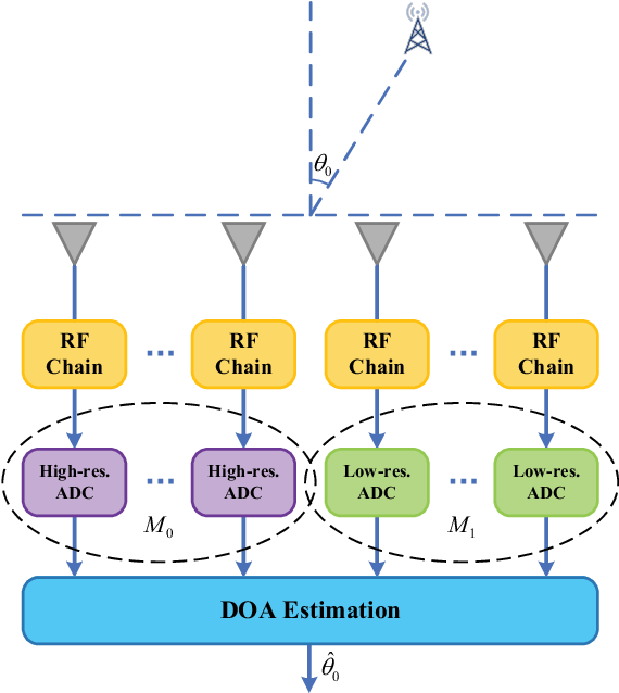
As shown in Fig 1, we consider a uniform linear array (ULA) equipped with mixed-ADCs. The array has $M_{0}$ high-resolution ADCs and $M_{1}$ low-resolution ADCs. The ULA has $M$ antenna elements, and we define $\kappa\triangleq M_{0}/M(0\leq\kappa\leq 1)$ as the proportion of high-resolution ADCs in the mixed-ADC architecture where $M=M_{0}+M_{1}$. The signal vector before quantization is given by

where $\mathbf{w}(t)\sim\mathcal{CN}(0,\mathbf{I}_{M})$ is the additive white Gaussian noise (AWGN), $s(t)$ is the received far-field narrow-band signal and $\mathbf{a}(\theta_{0})$ is the so-called array manifold, defined by

where $\Psi_{\theta_{0}}(m)=\frac{d_{m}\sin\theta_{0}}{\lambda}$ is the phase corresponding to the propagation delay of $m$th antenna element, where $\lambda$ is the wavelength of the signal.

For the ease of expression and analysis, the received signal is denoted as $\mathbf{x}(t)=[\mathbf{x}_{0}(t),~\mathbf{x}_{1}(t)]^{T}$, where $\mathbf{x}_{0}(t)$, $\mathbf{x}_{1}(t)$ are the $M_{0}\times 1$ and $M_{1}\times 1$ vector, which denote the signals that will be quantized by high-resolution ADCs and low-resolution ADCs, respectively. Thus, the received signals experiencing the $M_{0}$ high-resolution ADCs can be written as $\mathbf{y}_{0}(n)=\mathbf{x}_{0}(t)|_{t=n}=\mathbf{a}_{0}(\theta_{0})s(n)+\mathbf{w}_{0}(n),~n=1,2,\cdots,N,$ where $N$ is the number of snapshots. Furthermore, by leveraging on AQNM [9], the received signals quantized by $b$-bit ADCs can be formulated as

where $\mathbf{w}_{q}(n)$ denotes the quantization noise, $\mathbb{Q}(\cdot)$ is the quantization function, and $\alpha=1-\beta$ is the linear quantization gain, where $\beta=\frac{\mathbb{E}\left[\|\mathbf{x}_{1}-\mathbf{y}_{1}\|^{2}\right]}{\mathbb{E}\left[\|\mathbf{x}_{1}\|^{2}\right]}$ denotes the distortion factor of the low-resolution ADC. The accurate value of $\beta$ is listed in Table I when $b\leq 5$. For longer quantization bitlength (e.g., $b>5$), the distortion factor $\beta$ can be approximated as $\beta\approx\frac{\sqrt{3}\pi}{2}\cdot 2^{-2b},~b\geq 6.$ For a fixed channel realization, the covariance matrix of $\mathbf{w}_{q}$ is given by

Thus, $\mathbf{w}_{q}$ can be modelled as $\mathbf{w}_{q}\sim\mathcal{CN}(0,\mathbf{R}_{\mathbf{w}_{F}})$.

Thus, the overall received signal can be expressed as

The MUSIC proposed in [3] is a well-known subspace-based method for DOA estimation. In this section, we prove the fact that there is no change on MUSIC method.

When the array is equipped with pure high-resolution ADCs, the eigenvalue decomposition (EVD) of the covariance matrix $\mathbf{R}_{\mathbf{y}}^{\prime}$ can be written as

where the columns of $\mathbf{E}_{S}$ and $\mathbf{E}_{W}$ are the eigenvectors corresponding to the useful signal and channel noise, respectively. Those can span the signal subspace and noise subspace, which are orthogonal. Thus, the spectrum,

will be infinity when $\theta=\theta_{0}$. In practice, $\mathbf{R}_{\mathbf{y}}$ is estimated from sampled data by $\hat{\mathbf{R}}_{\mathbf{y}}=\frac{1}{N}\sum_{n=1}^{N}\mathbf{y}(n)\mathbf{y}^{H}(n).$

In mixed-ADC structure, the covariance matrix $\mathbf{R}_{\mathbf{y}}$ can be casted as (II) at the bottom of next page, where $\gamma=\mathbb{E}[ss^{H}]=\sigma_{s}^{2}=\sigma_{s}^{2}/\sigma_{n}^{2}$ is the input SNR of ADCs. Observing (II), as the number of quantization bit increases, $\mathbf{R}_{\epsilon}\rightarrow\mathbf{0}_{M}$ and $\|\mathbf{R}_{\epsilon}\|\ll\|\mathbf{R}_{\mathbf{y}}^{\prime}\|$, $\mathbf{R}_{\mathbf{y}}\approx\mathbf{R}_{\mathbf{y}}^{\prime}$ and $\mathbf{R}_{\epsilon}$ can be considered as the error of $\mathbf{R}_{\mathbf{y}}^{\prime}$. Thus, $\mathbf{R}_{\mathbf{y}}\approx\mathbf{R}_{\mathbf{y}}^{\prime}$ and $\mathbf{R}_{\epsilon}$ can be considered as the error of $\mathbf{R}_{\mathbf{y}}^{\prime}$. Now, let $\mathbf{e}^{\prime}$ and $\lambda^{\prime}$ denote the eigenvalue and eigenvector of $\mathbf{R}_{\mathbf{y}}^{\prime}$, respectively. Then, we have $\mathbf{R}_{\mathbf{y}}^{\prime}\mathbf{e}^{\prime}=\lambda^{\prime}\mathbf{e}^{\prime}$, which can be regarded as the linear equations $\mathbf{R}_{\mathbf{y}}^{\prime}\mathbf{x}=\mathbf{b}$. And the condition number of $\mathbf{R}_{\mathbf{y}}^{\prime}$ is given by

Obviously, $\mathbf{R}_{\mathbf{y}}^{\prime}$ has a low condition number. And, we can conclude that $\mathbf{R}_{\mathbf{y}}^{\prime}$ and $\mathbf{R}_{\mathbf{y}}$ will have the approximate eigenvalues and eigenvectors. Thus, MUSIC and other subspace-based methods can be applied without modification, like root-MUSIC and ESPRIT [4].

In this section, to evaluate the performance of the massive MIMO for mixed-ADC architecture, we derive the CRLB for the mixed-ADC structure. Then, the performance loss factor and EE factor are firstly defined to seek a basic trade-off between the performance and power consumption in practical applications.

In this section, we provide the simulation results to analyse the impact of different $\kappa$ and $b$ on the performance loss $\eta_{PL}$. Furthermore, the simulation of MUSIC with $\kappa=1/4$ and different $b$ is conducted, where all results are averaged over 8000 Monte Carlo realizations. In all simulations, it is assumed that two emitters are located in $\theta_{0}^{1}=-45^{\circ}$ and $\theta_{0}^{2}=30^{\circ}$, the number of snapshots $K$ is 32 and the number of antenna elements $M$ is $128$.

In Fig. 2, performance loss over $\kappa$ is illustrated. We consider two common SNR: $\gamma=0dB$ and $\gamma=10dB$. Obviously, $\eta_{PL}$ decreases as $\kappa$ increases. If we set 1 dB as an acceptable minimum of performance loss, 1-bit ADCs could be considered when $\kappa>0.9$. For a medium value of $\kappa$ ($0.2<\kappa<0.9$), ADCs with 2-bit or 3-bit are more suitable. In addition, when $\kappa$ decreases to 0.2 below, 3-bit ADCs even 4-bit ADCs can be adopted to achieve a satisfactory performance. Of course, in some special cases, more or less quantization bit of ADCs should be chosen to meet the practical requirement.

Fig. 3 plots curves of MUSIC spectrum for mixed-ADC arrays with different quantization bits. It is seen that MUSIC spectrums of arrays with 1-bit ADCs and 2-bit have lower peaks at the same directions. That proves that MUSIC method can be applied for mixed-ADC structure without modification and low-resolution ADCs have an impact on performance. An insightful conclusion is that mix-ADC structure has the similar eigen-subspace.

The EE against the quantization bits is shown in Fig. 4. We adopt the classic values in massive MIMO systems: $P_{syc}=50.0~\mathrm{mW}$, $P_{LNA}=20~\mathrm{mW}$, $P_{mix}=30.3~\mathrm{mW}$, $P_{fil}=2.5~\mathrm{mW}$, $P_{IFA}=3~\mathrm{mW}$, $P_{AGC}=2~\mathrm{mW}$, $V_{dd}=3~\mathrm{V}$, $L_{min}=0.5~\mathrm{\mu m}$, $f_{cor}=1~\mathrm{MHz}$ and $B=20~\mathrm{MHz}$ as in [9] and [12]. 12-bit is chosen as the quantization bit of high-resolution ADCs. It is clear that all curves reach peaks when $b=2$ or $3$. After reaching peeks, all curves decrease as the $b$ increases. And, the EE increases as $\kappa$ decreases. However, the performance of the array with pure low-resolution ADCs is too poor to be adopted. Thus, an appropriate $\kappa$ with 1-4 bits’ low-resolution ADCs is more suitable in mixed-ADC structure.

In this paper, we built the DOA estimation for the ULA with mixed-ADC. Then, we proved that the subspace-based methods can be applied to this system without modification. Furthermore, we derived the CRLB and as the benchmark of the performance. Based on that, the performance loss and EE was investigated, which showed that 1-4 bits’ ADCs are good choices in most applications. Finally, the mixed-ADC structure can achieve a satisfactory performance of DOA estimation with much less circuit cost and power consumption.

[Derivation of CRLB for Full Digital Structure with Mixed-ADC]In this section, we derive the CRLB for the massive MIMO with mixed-ADCs. In accordance with [1], the corresponding Fisher information matrix (FIM) $\mathbf{F}$ can be written as

For convenient derivation, $s(n)$, $\mathbf{y}(n)$, $\mathbf{a}(\theta_{0})$ and $\mathbf{w}(n)$ are abbreviated as $s$, $\mathbf{y}$, $\mathbf{a}$ and $\mathbf{w}$ respectively in the following part. Now, to simplify the derivation, we reformulate $\mathbf{y}$ as

where

and

Then, the $\mathbf{R}_{\mathbf{y}}$ is given by

where

Thus,

where $\dot{\mathbf{a}}$ is the differential of $\mathbf{a}$ to $\theta_{0}$, which is derived as

where

Therefor, with the help of some properties of the trace in [13], FIM can be expressed as

where

In the following, resorting to the well-known Sherman-Morrison-Woodbury formula in [13], we can get

Let us define

Then, we can get

where

Accordingly, substituting (VI) into (27), $F_{a}$ is given by

Similar to the derivation of $F_{a}$, $F_{c}$ can be derived as follows,

Now, let us focus on the derivation of $F_{b}$. The first part of (28) can be given by

And, the second part is expressed as

where

Combining (VI) and (VI), $F_{b}$ in (28) is represented by

Finally, substitute VI), (VI) and (VI) into (VI), which yields

Therefore, the CRLB is given by

The derivation of CRLB for the massive MIMO system with mixed-ADCs is completed. $\hfill\blacksquare$

References

- [1] T. E. Tuncer and B. Friedlander, Classical and Modern Direction-of-Arrival Estimation. Academic Press, 2009.
- [2] F. Shu, X. Wu, J. Hu, J. Li, R. Chen, and J. Wang, “Secure and precise wireless transmission for random-subcarrier-selection-based directional modulation transmit antenna array,” IEEE J. Sel. Areas Commun., vol. 36, no. 4, pp. 890–904, 2018.
- [3] R. Schmidt, “A signal subspace approach to multiple emitter location and spectral estimation,” Ph. D. Dissertation. Stanford Univ., 1981.
- [4] R. Roy, A. Paulraj, and T. Kailath, “ESPRIT–a subspace rotation approach to estimation of parameters of cisoids in noise,” IEEE Transactions on Acoustics, Speech, and Signal Processing, vol. 34, no. 5, pp. 1340–1342, 1986.
- [5] F. Shu, Y. Qin, T. Liu, L. Gui, Y. Zhang, J. Li, and Z. Han, “Low-complexity and high-resolution DOA estimation for hybrid analog and digital massive MIMO receive array,” IEEE Trans. Commun., vol. 66, no. 6, pp. 2487–2501, 2018.
- [6] D. Hu, Y. Zhang, L. He, and J. Wu, “Low-complexity deep-learning-based DOA estimation for hybrid massive MIMO systems with uniform circular arrays,” IEEE Wireless Commun. Lett., vol. 9, no. 1, pp. 83–86, 2020.
- [7] B. Shi, N. Chen, X. Zhu, Y. Qian, Y. Zhang, F. Shu, and J. Wang, “Impact of low-resolution ADC on DOA estimation performance for massive MIMO receive array,” arXiv preprint arXiv:2011.00451, 2020.
- [8] J. Singh, O. Dabeer, and U. Madhow, “On the limits of communication with low-precision analog-to-digital conversion at the receiver,” IEEE Trans. Commun., vol. 57, no. 12, pp. 3629–3639, 2009.
- [9] J. Zhang, L. Dai, Z. He, S. Jin, and X. Li, “Performance analysis of mixed-ADC massive MIMO systems over rician fading channels,” IEEE J. Sel. Areas Commun., vol. 35, no. 6, pp. 1327–1338, 2017.
- [10] N. Liang and W. Zhang, “Mixed-ADC massive MIMO,” IEEE J. Sel. Areas Commun., vol. 34, no. 4, pp. 983–997, 2016.
- [11] E. Lauwers and G. Gielen, “Power estimation methods for analog circuits for architectural exploration of integrated systems,” IEEE Trans. Very Large Scale Integr. (VLSI) Syst., vol. 10, no. 2, pp. 155–162, 2002.
- [12] Shuguang Cui, A. J. Goldsmith, and A. Bahai, “Energy-constrained modulation optimization,” IEEE Trans. Wireless Commun., vol. 4, no. 5, pp. 2349–2360, 2005.
- [13] X. Zhang, Matrix analysis and applications. Cambridge University Press, 2017.