Neutron Stars in Scalar-tensor Gravity with Quartic Order Scalar Potential

Neutron stars (NS) have developed to be in the epicenter of current scientific interest, since they are literally laboratories in the cosmos, for many scientific disciplines like nuclear Tolos:2020aln; Lattimer:2012nd; Steiner:2011ft; Horowitz:2005zb; Watanabe:2000rj; Shen:1998gq; Xu:2009vi; Hebeler:2013nza; Mendoza-Temis:2014mja; Ho:2014pta; Kanakis-Pegios:2020kzp and high energy particle physics Buschmann:2019pfp; Safdi:2018oeu; Hook:2018iia; Edwards:2020afl; Nurmi:2021xds, modified gravity Astashenok:2020qds; Capozziello:2015yza; Astashenok:2014nua; Astashenok:2014pua; Astashenok:2013vza; Arapoglu:2010rz; Astashenok:2020cqq and astrophysics Sedrakian:2015krq; Khadkikar:2021yrj; Sedrakian:2006zza; Sedrakian:2018kdm; Bauswein:2020kor; Vretinaris:2019spn; Bauswein:2020aag; Bauswein:2017vtn; Most:2018hfd; Rezzolla:2017aly. Nearly fifty years after the first observation of a NS by Jocelyn Bell, the observational aspects of neutron stars have been developed quite significantly, with the LIGO-Virgo collaboration being the “tip of the spear” in observing and analyzing gravitational waves emerging from NSs and black holes processes. Thus the aim of understanding the inner processes of neutron stars physics, which was scientifically a dream some decades ago, has developed to be every day physics nowadays. The LIGO-Virgo collaboration has set the stage for future discoveries, and the upcoming LISA collaboration is expected to further improve our knowledge on astrophysical and cosmological gravitational waves. Even the early results of the LIGO-Virgo collaboration has proven gold for both astrophysics and theoretical astrophysics, for example the pioneering 2017 observation known as GW170817 event TheLIGOScientific:2017qsa has indicated that the gravitational waves propagate with a speed that is nearly equal to that of light’s in vacuum. This result was obtained because luckily the GW170817 event was accompanied by a kilonova originating electromagnetic radiation which arrived almost simultaneously with the gravitational waves. From a theoretical point of view, this observation has excluded quite many theoretical cosmology models which predicted a gravitational wave speed different than that of light’s, although rectifications of problematic theories can be constructed in order for them to comply with the GW170817 event, see for example Odintsov:2020sqy; Oikonomou:2020sij. In addition, the GW190814 event Abbott:2020khf had a mysterious secondary component with mass in the range of the so-called mass-gap region. If this secondary component is proved to be a neutron star, or even a black hole, it will be a result of fundamental importance. In addition, fundamental particle physics models could be tested from pulsars observations, like the axion models that may be transformed to photons in the strong atmospheric magnetic fields of pulsars Hook:2018iia. Of course, observations may provide useful insights towards the understanding of nuclear matter equation of state (EoS) at high compression and at supranuclear densities. For a mainstream of textbooks and reviews on neutron stars, we refer the reader to Refs. Haensel:2007yy; Friedman:2013xza; Baym:2017whm; Lattimer:2004pg; Olmo:2019flu.

In view of the GW190814 event, the possibility of having a neutron star in the mass-gap region is rather scientifically stimulating, since such a result is marginally supported by general relativity (GR) even for the stiffest equation of state. For some interesting perspectives for the GW190814 event see Nathanail:2021tay; Koppel:2019pys. In the literature there exist several EoSs that may predict maximum masses for NSs that could describe the GW190814 event, but only marginally for the moment. However, if future observations indicate the existence of NSs masses in the mass-gap region, above $M\geq 2.6M_{\odot}$, this will indicate that GR may be complemented theoretically by an alternative description. Modified gravity Nojiri:2017ncd; Capozziello:2011et; Capozziello:2010zz; Nojiri:2006ri; Nojiri:2010wj; delaCruzDombriz:2012xy; Olmo:2011uz; dimo in its various forms may play some fundamental role if this scenario proves true, and in the literature there exist several descriptions of NSs with masses that cannot be reached by even the stiffest GR EoSs Astashenok:2014nua. In addition, in the context of modified gravity, some puzzles of ordinary GR descriptions of NSs, may be consistently resolved, such as the hyperon puzzle Astashenok:2014pua. The inner core of neutron stars is a mystery, and the existence of hyperons is softening significantly the EoS (if the two hyperon interaction is only taken into account), thus a large mass neutron star will indicate that a hyperon-free EoS must be used, but modified gravity can also harbor hyperon-related EoSs and simultaneously producing large masses for NSs Astashenok:2014pua. It is interesting to note though that for static neutron stars, even in the context of modified gravity one does not expect the maximum masses to be larger than $3\,M_{\odot}$ Astashenok:2021peo.

Modified gravity can serve as a successful complement of GR when large mass NSs are considered. In cosmology the urge for a modified gravity description of several phenomena is compelling, since dark energy and some aspects of inflation cannot be described by GR. With regard to dark energy, the most successful description of it, the $\Lambda$-Cold-Dark-Matter model heavily relies on the existence of a cosmological constant, which is constant so the dark energy EoS is exactly on the phantom divide line. However, the latest Planck data on cosmological parameters Aghanim:2018eyx indicate that range of values that the dark energy EoS, namely $\omega_{DE}$, is allowed to take, crosses the phantom divide line marginally towards the phantom regime, and specifically $\omega_{DE}=-1.018\pm 0.031$. Such a phantom possibility can of course be described by GR, but only by using a phantom scalar field Caldwell:2003vq, which is not an elegant and self-consistent description for a physical system. With regard to inflation, it is basically a classical era, a post-quantum era however, very close chronically and energy-wise to the quantum epoch of our Universe. The most popular description of inflation makes use of a scalar field, which is basically a GR description, but it is highly likely that the quantum era might leave its imprints on the inflationary Lagrangian, in terms of non-minimal couplings of scalars with gravity, couplings of scalars with higher order curvature terms, or Gauss-Bonnet couplings or even higher order curvature terms, see the reviews Nojiri:2017ncd; Capozziello:2011et; Capozziello:2010zz; Nojiri:2006ri; Nojiri:2010wj; delaCruzDombriz:2012xy; Olmo:2011uz; dimo for a complete description of all the possibilities for the effective inflationary Lagrangian.

In this paper we shall consider one of the above aspects for the Lagrangian of gravity, that of non-minimal couplings of scalar fields on gravity. We shall thus investigate scalar-tensor theories with non-minimal coupling of the scalar field with the Ricci scalar. We aim to study the hydrodynamic stability of static NSs for a specific physically motivated Lagrangian, and to find the quantities related to the hydrodynamic stability of NSs. The scalar-tensor theory we shall use is related to a quartic order scalar potential, which as a scalar-tensor theory is quite popular due to its similarity to the Higgs inflationary potential in cosmological contexts Bezrukov:2014bra; GarciaBellido:2011de; Bezrukov:2010jz; Bezrukov:2007ep; Mishra:2018dtg; Steinwachs:2013tr; Rubio:2018ogq; Kaiser:1994vs; Gundhi:2018wyz; CervantesCota:1995tz; Kamada:2012se; Schlogel:2014jea; Fuzfa:2013yba, since it can generate a successful inflationary era compatible with the latest Planck data on inflation Akrami:2018odb. As a scalar theory, our motivation for studying the a quartic order scalar model is not accidental at all. Thus, since its inflationary aspects provide a successful description of inflation, in this paper we shall consider the implications of the quartic order scalar model Lagrangian on static NSs. Our approach and notation will be technically similar to many studies of theoretical astrophysics approaches for scalar tensor theories Pani:2014jra; Staykov:2014mwa; Horbatsch:2015bua; Silva:2014fca; Doneva:2013qva; Xu:2020vbs; Salgado:1998sg; Shibata:2013pra; Arapoglu:2019mun; Ramazanoglu:2016kul; AltahaMotahar:2019ekm; Chew:2019lsa; Blazquez-Salcedo:2020ibb; Motahar:2017blm, and we shall use the notation of such approaches in order to comply with the existing literature. For a recent similar work in the same spirit as the present article see Odintsov:2021qbq. So we shall extract the Tolman-Oppenheimer-Volkoff (TOV) equations in the Einstein frame, and we shall calculate the gravitational masses of the NSs and the radii for several piecewise polytropic equations of state which are valid up to large central densities Read:2008iy; Read:2009yp. Our results will be the Jordan frame quantities, regarding the circumferential radii of the NSs, and with regard to the mass, since there are several different possibilities for the definition of the gravitational mass, such as the Komar mass Komar:1958wp, in this paper we shall use the Arnowitt-Deser-Misner (ADM) mass Arnowitt:1960zzc, which for static stellar configurations coincide Shibata:2013ssa. For the solution of the TOV equations, we shall use the well known numerical code pyTOV-STT niksterg, appropriately modified to incorporate the scalar potential, and we shall use a double shooting method in order to most accurate values for the scalar field and one of the two metric related functions. In addition, before getting to the core of this study, we shall present in brief the cosmologist’s and theoretical astrophysicist’s perspective of scalar-tensor theories, since there is a difference in notation, which might cause confusion initially to a cosmologist, but for the calculations we shall use the usual theoretical astrophysics notation and physical units, with all the quantities of interest converted in the end in the CGS system. As for the values of the free parameters, these shall be aligned with the values imposed by the inflationary constraints. We need to mention that NSs with similar potential in the Jordan frame were studied in Arapoglu:2019mun, but our approach is different since we deal with the Einstein frame theory, plus we use a physically motivated from inflation Einstein frame scalar field potential.

This paper is organized as follows: In section II we present the cosmologist’s perspective of scalar-tensor theory in the Jordan and Einstein frame, where the natural units physical system is used. In section II, we present the theoretical astrophysicist’s perspective of the scalar-tensor gravity in geometrized units, and we shall try to bridge the two approaches in order to make direct correspondence with the inflationary quartic order scalar model, always in geometrized units. In section III, we describe in brief the essential features of the piecewise polytropic equation of state approach, and in section IV we study in detail the quartic order scalar model potential in the Einstein frame for compact static spherically symmetric stellar objects. We derive the TOV equations in the Einstein frame and by using a well-known python-based numerical code, which we appropriately modified to incorporate the scalar potential, we numerically solve the TOV equations using a double shooting method for maximum accuracy of the delivered results. In the same section we present the results of our analysis for several piecewise polytropic EoSs of interest, and for various values of the free parameters, and finally we directly compare the results with the GR ones. Also we examine the values of the scalar field in the Jordan frame and we investigate whether the approximations needed are satisfied by the numerical results. Finally, the conclusions follow at the end of the paper.

The notation used for scalar-tensor theory in cosmological contexts is different from the one used in theoretical astrophysics context. Therefore, we shall present both frameworks in order to bridge the gap between the two contexts, since we shall make a direct correspondence of the quartic order scalar inflationary model from the cosmological context to a theoretical astrophysics context. In this section we shall present the cosmologist’s perspective of scalar-tensor theories, using natural units. Details for the formalism used can be found in Refs. Kaiser:1994vs; valerio; Faraoni:2013igs; Buck:2010sv; Faraoni:1998qx; Odintsov:2021qbq.

Consider the Jordan frame action in the presence of the non-minimally coupled inflaton and the matter Lagrangian,

$$\mathcal{S}_{J}=\int d^{4}x\Big[f(\phi)R-\frac{1}{2}g^{\mu\nu}\partial_{\mu}\phi\partial_{\nu}\phi-U(\phi)\Big]+S_{m}(g_{\mu\nu},\psi_{m})\,,$$

(1)

where $\psi_{m}$ denotes the perfect matter fluids present in the Jordan frame, with pressure $P$ and energy density $\epsilon$, and $g_{\mu\nu}$ the Jordan frame metric. The minimal coupling choice corresponds to,

$$f(\phi)=\frac{1}{16\pi G}=\frac{M_{p}^{2}}{2}\,,$$

(2)

where,

$$M_{p}=\frac{1}{\sqrt{8\pi G}}\,,$$

(3)

is the Jordan frame reduced Planck mass, which is $M_{p}=2.43\times 10^{18}$GeV, and $G$ is Newton’s gravitational constant in the Jordan frame. Now we shall perform a conformal transformation of the following form,

$$\tilde{g}_{\mu\nu}=\Omega^{2}g_{\mu\nu}\,,$$

(4)

or equivalently,

$$\tilde{g}^{\mu\nu}=\Omega^{-2}g^{\mu\nu}$$

(5)

in order to obtain the action in the Einstein frame. Hereafter, the tilde will denote quantities in the Einstein frame. Also $\Omega$ in terms of $f(\phi)$ is written as Kaiser:1994vs; Mishra:2018dtg; valerio,

$$\Omega^{2}=\frac{2}{M_{p}^{2}}f(\phi)\,.$$

(6)

The quantities appearing in the Jordan frame action are transformed in the following way,

$$\sqrt{-g}=\Omega^{-4}\sqrt{-\tilde{g}}\,,$$

(7)

the Ricci scalar transforms as follows,

$$R=\Omega^{2}\left(\tilde{R}+6\tilde{\square}f-6\tilde{g}^{\mu\nu}f_{\mu}f_{\nu}\right)\,,$$

(8)

and the d’Alembertian is,

$$\tilde{\square}f=\frac{1}{\sqrt{-\tilde{g}}}\tilde{\partial}_{\mu}\left(\sqrt{-\tilde{g}}\tilde{g}^{\mu\nu}\partial_{\nu}f\right)\,.$$

(9)

Thus the non-minimal coupling term is transformed in the Einstein frame as follows,

$$\int d^{4}x\sqrt{-g}f(\phi)R\to\int d^{4}x\sqrt{-\tilde{g}}\frac{M_{p}^{2}}{2}\left(\tilde{R}-6\left(\frac{1}{\Omega^{2}}\right)^{2}\tilde{g}^{\mu\nu}\tilde{\partial}_{\mu}\Omega\tilde{\partial}_{\nu}\Omega\right)\,,$$

(10)

and the Jordan frame kinetic term plus the potential term transform as follows,

$$\int d^{4}x\sqrt{-g}\Big[-\frac{1}{2}g^{\mu\nu}\partial_{\mu}\phi\partial{\nu}-U(\phi)\Big]+S_{m}(g_{\mu\nu},\psi_{m})\to\int d^{4}x\sqrt{-\tilde{g}}\Big[-\frac{1}{2\Omega^{2}}\tilde{g}^{\mu\nu}\tilde{\partial}_{\mu}\phi\tilde{\partial}{\nu}\phi-\frac{U(\phi)}{\Omega^{4}(\varphi)}\Big]+S_{m}(\Omega^{2}\tilde{g}_{\mu\nu},\psi_{m})$$

(11)

thus in the end, the Einstein frame action in terms of $\Omega^{2}=\frac{2}{M_{p}^{2}}f$ becomes,

$$\mathcal{S}_{E}=\int d^{4}x\sqrt{-\tilde{g}}\Big[\frac{M_{p}^{2}}{2}\tilde{R}-\frac{\zeta(\phi)}{2}\tilde{g}^{\mu\nu}\tilde{\partial}_{\mu}\phi\tilde{\partial}_{\nu}\phi-V(\phi)\Big]+S_{m}(\Omega^{-2}\tilde{g}_{\mu\nu},\psi_{m})\,,$$

(12)

where,

$$V(\phi)=\frac{U(\phi)}{\Omega^{4}}\,,$$

(13)

and also we introduced $\zeta(\phi)$ which is,

$$\zeta(\phi)=\frac{3}{2}M_{p}^{2}\frac{1}{f^{2}}\Big(\frac{df}{d\phi}\Big)^{2}+\frac{M_{p}^{2}}{2f}\,.$$

(14)

In addition, clearly the Einstein frame scalar field $\phi$ is not canonical since $\zeta(\phi)\neq 1$, hence we perform the following rescaling,

$$\Big(\frac{d\varphi}{d\phi}\Big)^{2}=\zeta(\phi)\,,$$

(15)

or equivalently,

$$\frac{d\varphi}{d\phi}=M_{p}\sqrt{\frac{1}{2f}+\frac{3}{2}\Big(\frac{f^{\prime}}{f}\Big)^{2}}\,,$$

(16)

where the prime indicates differentiation with respect to $\phi$, that is $f^{\prime}=\frac{df}{d\phi}$. Hence the Einstein frame action in terms of the canonical scalar field $\varphi$ reads,

$$\mathcal{S}_{E}=\int d^{4}x\sqrt{-\tilde{g}}\Big[\frac{M_{p}^{2}}{2}\tilde{R}-\frac{1}{2}\tilde{g}^{\mu\nu}\tilde{\partial}_{\mu}\varphi\tilde{\partial}_{\nu}\varphi-V(\varphi)\Big]+S_{m}(\Omega^{2}\tilde{g}_{\mu\nu},\psi_{m})$$

(17)

where,

$$V(\varphi)=\frac{U(\varphi)}{\Omega^{4}}=\frac{U(\varphi)}{4M_{p}^{4}f^{2}}\,.$$

(18)

Clearly, the fluids $\psi_{m}$ in the Einstein frame are not perfect, due to the presence of the conformal factor in the matter action, hence, the energy momentum tensor which is,

$$\tilde{T}_{\mu\nu}=-\frac{2}{\sqrt{-\tilde{g}}}\frac{\delta L_{m}}{\delta\tilde{g}^{\mu\nu}}\,,$$

(19)

from the Jordan frame to the Einstein frame transforms as,

$$\tilde{T}_{\mu\nu}=\Omega^{-2}(\varphi)T_{\mu\nu}\,,$$

(20)

$$\tilde{T}^{\mu}_{\nu}=\Omega^{-4}(\varphi)T^{\mu}_{\nu}\,,$$

(21)

$$\tilde{T}^{\mu\nu}=\Omega^{-6}(\varphi)T^{\mu\nu}\,,$$

(22)

and the trace of the energy momentum tensor transforms as,

$$\tilde{T}=\Omega^{-4}T\,.$$

(23)

The continuity equation for the energy momentum tensor in the Einstein frame reads,

$$\tilde{\partial}^{\mu}\tilde{T}_{\mu\nu}=-\frac{d}{d\varphi}[\ln\Omega]\tilde{T}\tilde{\partial}_{\nu}\phi\,.$$

(24)

In the Jordan frame, where the matter fluids are perfect fluids, the energy momentum tensor takes the form,

$$T_{\mu\nu}=(P+\varepsilon)u_{\mu}u_{\nu}+Pg_{\mu\nu}\,,$$

(25)

where $P$ and $\varepsilon$ are the Jordan frame pressure and energy momentum respectively, and suppose that in the Einstein frame the energy momentum tensor is,

$$\tilde{T}_{\mu\nu}=(\tilde{P}+\tilde{\varepsilon})\tilde{u}_{\mu}\tilde{u}_{\nu}+\tilde{P}\tilde{g}_{\mu\nu}\,,$$

(26)

where the Einstein frame pressure is denoted as $\tilde{P}$ and the corresponding Einstein frame energy density is $\tilde{\varepsilon}$. The four-velocity $\tilde{u}_{\mu}$ satisfies,

$$\tilde{g}_{\mu\nu}\tilde{u}^{\mu}\tilde{u}^{\nu}=-1\,.$$

(27)

Thus, the four-velocity transforms as $\tilde{u}_{\mu}=\Omega^{1}u_{\mu}$, and by direct comparison of the energy momentum tensors in the Jordan and the Einstein frame, we get that the pressure and the energy density in the two frames are related as follows,

$$\tilde{\varepsilon}=\Omega^{-4}(\varphi)\varepsilon,\,\,\,\tilde{P}=\Omega^{-4}(\varphi)P\,.$$

(28)

In the context of theoretical astrophysics, a different notation for the gravitational action and conformal transformation is used, leading to different dimensions of the scalar field, since the Geometrized units are used usually ($G=c=1$). This formalism and notation is commonly used in most of the theoretical astrophysics works. In the following we shall use the notation and formalism of Pani:2014jra, with the only difference being that the tilde notation will indicate quantities in the Einstein frame, contrary to Ref. Pani:2014jra, where the Jordan frame quantities are denoted with a “tilde”.

To start with consider the non-minimally coupled scalar field action in the Jordan frame (note our difference in the usage of the tilde, in order to provide a uniform notation for the present work) Pani:2014jra,

$$\mathcal{S}=\int d^{4}x\frac{\sqrt{-g}}{16\pi G}\Big[f(\phi)R-\frac{1}{2}g^{\mu\nu}\partial_{\mu}\phi\partial_{\nu}\phi-U(\phi)\Big]+S_{m}(\psi_{m},g_{\mu\nu})\,,$$

(29)

where $\phi$ denotes the scalar field in the Jordan frame. We shall use Geometrized units in which $c=G=1$, and we shall make the conformal transformation,

$$\tilde{g}_{\mu\nu}=A^{-2}g_{\mu\nu}\,,$$

(30)

where recall that the tilde denotes quantities in the Einstein frame. The function $A(\phi)$ is arbitrary, but for the choice,

$$A(\phi)=f^{-1/2}(\phi)\,,$$

(31)

one obtains a minimally coupled scalar field in the Einstein frame. So from now on we shall assume that $A(\phi)=f^{-1/2}(\phi)$, and in addition, the scalar potential in the Einstein frame is,

$$V(\phi)=\frac{U(\phi)}{f^{2}(\phi)}\,,$$

(32)

but the resulting action contains a non-canonical kinetic term for the scalar field $\phi$, which can be made canonical by making the following simple transformation,

$$\Big(\frac{d\varphi}{d\phi}\Big)=\frac{1}{\sqrt{4\pi}}\sqrt{\Big(\frac{3}{4}\frac{1}{f^{2}}\Big(\frac{df}{d\phi}\Big)^{2}+\frac{1}{4f}\Big)}\,,$$

(33)

where $\varphi$ is the canonical scalar field in the Einstein frame, hence the gravitational action in the Einstein frame becomes in terms of the canonical scalar field $\varphi$,

$$\mathcal{S}=\int d^{4}x\sqrt{-\tilde{g}}\Big(\frac{\tilde{R}}{16\pi}-\frac{1}{2}\tilde{g}_{\mu\nu}\partial^{\mu}\varphi\partial^{\nu}\varphi-\frac{V(\varphi)}{16\pi}\Big)+S_{m}(\psi_{m},A^{2}(\varphi)g_{\mu\nu})\,.$$

(34)

In the Einstein frame, the field equations for a general metric $\tilde{g}_{\mu\nu}$ read,

$$\tilde{G}_{\mu\nu}=8\pi\tilde{T}_{\mu\nu}+8\pi\Big(\tilde{\partial}_{\mu}\varphi\tilde{\partial}_{\nu}\varphi-\frac{\tilde{g}_{\mu\nu}}{2}\tilde{\partial}_{\sigma}\varphi\tilde{\partial}^{\sigma}\varphi\Big)-\frac{\tilde{g}_{\mu\nu}}{2}V(\varphi)\,,$$

(35)

$$\tilde{\square}\varphi=-\frac{A^{\prime}(\varphi)}{A(\varphi)}\tilde{T}+\frac{V^{\prime}(\varphi)}{16\pi}\,,$$

(36)

where $\tilde{T}$ is the trace of the energy momentum tensor in the Einstein frame. The energy momentum tensor in the Einstein frame $\tilde{T}^{\mu\nu}$ is related to the perfect fluid energy momentum tensor of the Jordan frame $T_{\mu\nu}$ as follows,

$$\tilde{T}_{\mu\nu}=A^{2}T_{\mu\nu}\,,$$

(37)

$$\tilde{T}^{\mu}_{\nu}=A^{4}T^{\mu}_{\nu}\,,$$

(38)

and the traces are related as follows,

$$\tilde{T}=A^{4}T\,,$$

(39)

therefore the pressure $\tilde{P}$ and the energy density $\tilde{\epsilon}$ in the Einstein frame are related to the Jordan frame ones $P$ and $\epsilon$ as follows,

$$\tilde{\epsilon}=A^{4}\epsilon\,,$$

(40)

$$\tilde{P}=A^{4}P\,.$$

(41)

In the cosmological applications, in natural units ($c=\hbar=1$), the various physical quantities have the following dimensions,

		$\displaystyle x^{\mu}=[m]^{-1}\,,\,\,\,\tilde{\partial}_{\mu}=[m]$		(42)
		$\displaystyle\tilde{R}=[m]^{2}\,,\,\,\,\frac{1}{G}=[m]^{2}$
		$\displaystyle V(\varphi)=[m]^{4}\,,\,\,\,\varphi=[m]$

In the astrophysical contexts, where the more appropriate Geometrized Units are used ($G=c=1$), the scalar field is dimensionless. The TOV equations eventually will be presented in the Geometrized Units. If we start from the action of the cosmological contexts, namely,

$$\mathcal{S}_{E}=\int d^{4}x\sqrt{-\tilde{g}}\Big[\frac{M_{p}^{2}}{2}\tilde{R}-\frac{1}{2}\tilde{g}^{\mu\nu}\tilde{\partial}_{\mu}\varphi\tilde{\partial}_{\nu}\varphi-V(\varphi)\Big]\,,$$

(43)

it can be brought in the form,

$$\mathcal{S}_{E}=\int d^{4}x\sqrt{-\tilde{g}}\frac{1}{16\pi G}\Big[\tilde{R}-\frac{1}{2}\tilde{g}^{\mu\nu}\tilde{\partial}_{\mu}\tilde{\varphi}\tilde{\partial}_{\nu}\tilde{\varphi}-V(\tilde{\varphi})\Big]\,,$$

(44)

by rescaling the scalar field $\varphi$ as follows,

$$\tilde{\varphi}=\sqrt{16\pi G}\varphi=\frac{\sqrt{2}}{M_{p}}\varphi\,.$$

The above notation for the action is unusual, meaning that the factor $1/(16\pi G)$ does not multiply the whole action, just the Ricci scalar. In theoretical astrophysics contexts, the action appears with an overall multiplicative factor $1/(16\pi G)$, so this is what we also adopt for this work.

For the present NS study in Einstein frame we shall consider a piecewise polytropic EoS Read:2008iy; Read:2009yp (see also the introductory text of the TOV-pp code which can be found in niksterg), which we now describe in brief. A piecewise polytropic EoS consists of a low-density part $\rho<\rho_{0}$, which in general can be a tabulated crust EoS, and of a high density part with $\rho\gg\rho_{0}$. The density $\rho_{0}$ is a matching density between the low and high density pieces, and the piecewise polytropic EoS needs other two dividing high densities, $\rho_{1}=10^{14.7}{\rm g/cm^{3}}$ and $\rho_{2}=10^{15.0}{\rm g/cm^{3}}$. The density and pressure in each of the piecewise density interval $\rho_{i-1}\leq\rho\leq\rho_{i}$ satisfy the following the polytropic relation,

$$P=K_{i}\rho^{\Gamma_{i}}\,,$$

(45)

and the requirement is that continuity is necessary at the crossing points of each piece. Particularly, at a dividing density $\rho_{i}$, the following continuity relations must hold true,

$$P(\rho_{i})=K_{i}\rho^{\Gamma_{i}}=K_{i+1}\rho^{\Gamma_{i+1}}\,,$$

(46)

and from the above continuity relations we can obtain the parameters $K_{2}$ and $K_{3}$ for a given chosen $K_{1},\Gamma_{1},\Gamma_{2},\Gamma_{3}$, or equivalently for a given initial pressure $p_{1}$ and for given parameters $\Gamma_{2}$, and $\Gamma_{3}$, which are not chosen arbitrarily. For the purposes article, the initial pressure $p_{1}$ and the parameters $\Gamma_{2}$, and $\Gamma_{3}$ will correspond to the values of three distinct EoSs, the WFF1 Wiringa:1988tp which is a variational method EoS, the SLy Douchin:2001sv which is a potential method EoS, and the APR EoS Akmal:1998cf. Upon integrating the first law of thermodynamics for barotropic fluids,

$$d\frac{\epsilon}{\rho}=-Pd\frac{1}{\rho}\,,$$

(47)

and the continuity requirement in the energy density, gives,

$$\epsilon(\rho)=(1+\alpha_{i})\rho+\frac{K_{i}}{\Gamma_{i}-1}\rho^{\Gamma_{i}}\,,$$

(48)

for $\Gamma_{i}\neq 1$, where,

$$\alpha_{i}=\frac{\epsilon(\rho_{i-1})}{\rho_{i-1}}-1-\frac{K_{i}}{\Gamma_{i}-1}\rho_{i-1}^{\Gamma_{i}-1}\,.$$

(49)

Moreover, the sound speed $v_{s}=\sqrt{dP/d\epsilon}$ can be expressed in terms of the parameters of the piecewise EoS,

$$v_{s}(\rho)=\sqrt{\frac{\Gamma_{i}P}{\epsilon+P}}\,.$$

(50)

Let us now proceed to the core of this study, and we shall present the quartic order scalar model in the Jordan frame and the corresponding Einstein frame theory, and accordingly we shall present the field equations for the Einstein frame theory for a spherically symmetric and static spacetime. We shall use the astrophysical conventions and notation presented in section III, but also we shall make contact with the cosmological notation in order to make the appropriate choices for the values of the free parameters. In the following we shall adopt the notation of Pani:2014jra. The quartic order scalar model as is used in cosmological contexts Mishra:2018dtg, has the following Jordan frame action in Geometrized units ($G=1$ and we use the notation of Pani:2014jra),

$$\mathcal{S}=\int d^{4}x\frac{\sqrt{-g}}{16\pi}\Big[f(\phi)R-\frac{1}{2}g^{\mu\nu}\partial_{\mu}\phi\partial_{\nu}\phi-U(\phi)\Big]+S_{m}(\psi_{m},g_{\mu\nu})\,,$$

(51)

with the non-minimal coupling function $f(\phi)$ and the potential $U(\phi)$ being defined as follows,

$$f(\phi)=1+\xi\phi^{2}\,,$$

(52)

$$U(\phi)=\lambda\phi^{4}\,,$$

(53)

and with $\phi$ we obviously denote the Jordan frame scalar field. Note that such choice of potentials corresponds to multiplicatively-renormalizable scalar theory in curved spacetime serg2. Upon performing the conformal transformation,

$$\tilde{g}_{\mu\nu}=A^{-2}g_{\mu\nu}\,,$$

(54)

we obtain the Einstein frame action expressed in terms of the canonical scalar field $\varphi$,

$$\mathcal{S}=\int d^{4}x\sqrt{-\tilde{g}}\Big(\frac{\tilde{R}}{16\pi}-\frac{1}{2}\tilde{g}_{\mu\nu}\partial^{\mu}\varphi\partial^{\nu}\varphi-\frac{V(\varphi)}{16\pi}\Big)+S_{m}(\psi_{m},A^{2}(\varphi)g_{\mu\nu})\,,$$

(55)

and recall the “tilde” denotes Einstein frame quantities. For the quartic order scalar model, the function $A(\phi)$ appearing in the conformal transformation (54), is defined as follows,

$$A(\phi)=f^{-1/2}(\phi)\,,$$

(56)

thus by using Eq. (52) we have,

$$A(\phi)=\left(1+\xi\phi^{2}\right)^{-1/2}\,,$$

(57)

and in the end we shall express the function $A(\phi)$ as a function of the Einstein frame canonical scalar field $\varphi$, after we obtain the relation $\phi(\varphi)$. Accordingly, the Einstein frame potential is,

$$V(\phi)=\frac{U(\phi)}{f^{2}(\phi)}\,,$$

(58)

which in term of $\phi$ is,

$$V(\phi)=\frac{\lambda\phi^{4}}{\left(1+\xi\phi^{2}\right)^{2}}\,,$$

(59)

and in the end we shall express the potential as a function of the Einstein frame canonical scalar field $\varphi$. The relation between the Jordan frame scalar field $\phi$ and the Einstein frame canonical scalar field $\varphi$ is,

$$\frac{d\varphi}{d\phi}=\frac{1}{\sqrt{4\pi}}\sqrt{\Big(\frac{3}{4}\frac{1}{f^{2}}\Big(\frac{df}{d\phi}\Big)^{2}+\frac{1}{4f}\Big)}\,,$$

(60)

so by substituting $f(\phi)$ from Eq. (52), we get,

$$\frac{d\varphi}{d\phi}=\frac{1}{\sqrt{16\pi}}\frac{\sqrt{1+\xi\phi^{2}+12\xi^{2}\phi^{2}}}{1+\xi\phi^{2}}\,.$$

(61)

Standard approximations used in cosmological contexts for the above Eq. (61) are the following (see Eq. (73) later on in this section, and the relevant discussion below it),

$$\xi^{2}\phi^{2}\gg 1\,,$$

(62)

and simultaneously,

$$\xi^{2}\phi^{2}\gg\xi\phi^{2}\,,$$

(63)

with Eq. (63) holding automatically true for $\xi\gg 1$. Using the approximations (62) and (63), Eq. (61) becomes,

$$\frac{d\varphi}{d\phi}\simeq\frac{\sqrt{12}}{\sqrt{16\pi}}\frac{\xi\phi}{1+\xi\phi^{2}}=\frac{\sqrt{12}}{2\sqrt{16\pi}}\frac{f^{\prime}(\phi)}{f(\phi)}\,,$$

(64)

thus upon integration, Eq. (64) yields the relation between $\varphi$ and $\phi$ which is,

$$\varphi=\frac{\sqrt{12}}{2\sqrt{16\pi}}\ln\left(f(\phi)\right)=\frac{\sqrt{12}}{2\sqrt{16\pi}}\ln\left(1+\xi\phi^{2}\right)\,,$$

(65)

hence,

$$1+\xi\phi^{2}=e^{\frac{2\sqrt{16\pi}}{\sqrt{12}}\,\varphi}\,.$$

(66)

Thus from Eq. (57), we can express $A(\phi)$ as a function of the Einstein frame canonical scalar field $\varphi$ as follows,

$$A(\varphi)=e^{\alpha\varphi}\,,$$

(67)

where $\alpha$ is defined as,

$$\alpha=-2\sqrt{\frac{\pi}{3}}\,,$$

(68)

and in the scalar-tensor literature the function $\alpha(\varphi)$ is,

$$\alpha(\varphi)=\frac{d\ln A(\varphi)}{d\varphi}\,,$$

(69)

so in our case,

$$a(\varphi)=\alpha=-2\sqrt{\frac{\pi}{3}}\,.$$

(70)

Accordingly, the potential and it’s first derivative with respect to the Einstein frame canonical scalar field $\varphi$ are,

$$V(\varphi)\simeq\frac{\lambda}{\xi^{2}}\left(e^{2\alpha\varphi}-1\right)^{2}\,,$$

(71)

and,

$$V^{\prime}(\varphi)\simeq\frac{4\alpha\lambda}{\xi^{2}}e^{2\alpha\varphi}\left(e^{2\alpha\varphi}-1\right)\,.$$

(72)

The potential (71) is quite well known in cosmological contexts and yields viable inflationary phenomenology (see Eq. (43) of Ref. Mishra:2018dtg). As it is known from Ref. Mishra:2018dtg, the quartic order scalar inflationary model yields a viable inflationary phenomenology for,

$$\frac{\lambda M_{p}^{4}}{4\xi^{2}}\sim 9.6\times 10^{-11}M_{p}^{4}\,,$$

(73)

where $M_{p}=\frac{1}{\sqrt{8\pi G}}$. Making the correspondence in Geometrized units and using the notation of this section, in our notation the constraint (73) becomes,

$$\frac{\lambda}{\xi^{2}}\sim 16\pi\times\left(1.51982\times 10^{-13}\right)\,,$$

(74)

so by using $\lambda=0.1$ for quartic order scalar model phenomenological reasoning Mishra:2018dtg, this yields $\xi\sim 11.455\times 10^{4}$, hence, for the NS study we shall use the value $\xi\sim 11.455\times 10^{4}$, which yields a viable inflationary phenomenology.

With regard to the values of the coupling parameter $\xi$, there are some limits coming from different quantum field theories in curved spacetime serg2; serg1. Indeed, we consider quartic order scalar model scalar sector which basically is just sector of some realistic grand unified theory (GUT) in curved spacetime. There are different possibilities for GUTs at the very early Universe. Let us mention two classes of such GUTS: asymptotically-free GUTs and finite GUTs, for which some estimations for value of $\xi$ can be done. For other types of GUT less strict estimations maybe also developed. Specifically, by taking renormalization group arguments at high energy, one can estimate the effective coupling $\xi$ at very high curvature corresponding to the high energy or very early Universe. It turns out that this effective coupling constant $\xi$ at high energy depends on the specific class of GUT under consideration. For instance, for asymptotically free finite grand unified theories $\xi$ most usually tends to the value $\xi=1/6$, the conformal coupling value. In addition, for some asymptotically free GUTs, $\xi$ can be arbitrarily large and its explicit value depends on initial conditions serg2; serg1; serg3. For such class of GUTs the large behavior of $\xi$ is apparent for $\xi\sim 11.455\times 10^{4}$, the choice used in this work. In this case, the constraint (63) is always satisfied for all the values of the Einstein frame scalar field $\varphi$ (see relation (66)), but the first constraint is not automatically satisfied, namely Eq. (62). Moreover, for different finite GUTs one has the following possibilities at high energy: $\xi$ tends to the conformal coupling value $1/6$ (asymptotical conformal invariance), or $\xi$ tends to very large value, or $\xi$ is arbitrary and it is not defined by quantum field considerations. Eventually, the last two possibilities for the values of $\xi$ again support our choice for large $\xi$ under consideration in our estimation. Note that for effective quantum field theory we do not have such asymptotic limitations for $\xi$ and it should be derived by cosmological considerations.

It is apparent that for $\xi\sim 11.455\times 10^{4}$, the constraint (63) is always satisfied for all the values of the Einstein frame scalar field $\varphi$ (see relation (66)), but the first constraint is not automatically satisfied, namely Eq. (62). Thus, when the numerical results are obtained, which will deliver the values of the scalar field $\varphi$, one must use Eq. (66) to transform the Einstein frame scalar field to the Jordan frame expression $\xi\phi^{2}$, and thus eventually the following constraint must be satisfied for all the numerical values of the Einstein frame scalar field $\varphi$ that will be delivered from the numerical code,

$$\xi^{2}\phi^{2}=\xi\,\left(e^{\frac{2\sqrt{16\pi}}{\sqrt{12}}\,\varphi}-1\right)\gg 1\,.$$

(75)

Let us now derive the (TOV) equations for a spherically symmetric compact stellar object, described by the spherically symmetric static spacetime metric,

$$ds^{2}=-e^{\nu(r)}dt^{2}+\frac{dr^{2}}{1-\frac{2m}{r}}+r^{2}(d\theta^{2}+\sin^{2}\theta d\phi^{2})\,,$$

(76)

where the function $m(r)$ describes the gravitational mass of the stellar object confined inside a radius $r$.

Assuming the Geometrized physical units system in which $c=G=1$, the field equations for the Einstein frame action corresponding to the rescaled canonical scalar field $\varphi$, for the spherically symmetric metric (76) read,

$$\frac{dm}{dr}=4\pi r^{2}A^{4}(\varphi)\epsilon+2\pi r(r-2m)\omega^{2}+4\pi r^{2}V(\varphi)\,,$$

(77)

$$\frac{d\nu}{dr}=4\pi r\omega^{2}+\frac{2}{r(r-2m)}\Big[4\pi A^{4}(\varphi)r^{3}P-4\pi V(\varphi)r^{3}\Big]+\frac{2m}{r(r-2m)}\,,$$

(78)

$$\frac{d\omega}{dr}=\frac{rA^{4}(\varphi)}{r-2m}\Big(\alpha(\varphi)(\epsilon-3P)+4\pi r\omega(\epsilon-P)\Big)-\frac{2\omega(r-m)}{r(r-2m)}+\frac{8\pi\omega r^{2}V(\varphi)+r\frac{dV(\varphi)}{d\varphi}}{r-2m}\,,$$

(79)

$$\frac{dP}{dr}=-(\epsilon+P)\Big[\alpha(\varphi)\omega+2\pi r\omega^{2}+\frac{m-4\pi r^{3}(-A^{4}P+V)}{r(r-2m)}\Big]\,,$$

(80)

$$\frac{d\varphi}{dr}=\omega\,,$$

(81)

where the function $\alpha(\varphi)$ is defined in Eq. (70), and the potential and its derivative are defined in Eqs. (71) and (72) respectively. Also and the pressure $P$ and energy density $\epsilon$ in the TOV equations are the Jordan frame quantities. Clearly, the GR limit of the TOV equations is obtained by setting $A=1$, $\omega=0$, $\alpha(\varphi)=0$, $V=0$ and of course $\frac{dV}{d\varphi}=0$. The TOV equations for the scalar-tensor theory in the Einstein frame must be solved for the following initial conditions,

$$P(0)=P_{c}\,,$$

(82)

$$m(0)=0\,,$$

(83)

$$\nu(0)\,,=-\nu_{c}$$

(84)

$$\varphi(0)=\varphi_{c}\,,$$

(85)

$$\omega(0)=0\,.$$

(86)

Near the center the pressure, mass and the metric function have the following Taylor expansions,

$$P(r)\simeq P_{c}-(2\pi)(\epsilon_{c}+P_{c})\left(P_{c}+\frac{1}{3}\epsilon_{c}\right)r^{2}+O(r^{4})\,,$$

(87)

$$m(r)\simeq\frac{4}{3}\pi\epsilon_{c}r^{3}+O(r^{4})\,,$$

(88)

$$\nu(r)\simeq\nu_{c}+4\pi\left(P_{c}+\frac{1}{3}\epsilon_{c}\right)r^{2}+O(r^{4})\,.$$

(89)

In the present section we shall perform a numerical integration of the TOV equations, using the initial conditions above and using a double shooting method in order to obtain the optimal central values for the variable $\nu_{c}$ and the value of the scalar field $\varphi_{c}$ at the center of the NS, which make the scalar field $\varphi(r)$ and the metric function $\nu(r)$ vanish at the numerical infinity which is chosen to be $r\sim 67.943$ km in the Einstein frame. The gravitational mass of the star will be assumed to be the ADM mass measured in solar masses. Let us derive the ADM mass for the scalar-tensor theory at hand, and specifically the Jordan frame mass. Let us introduce some notation at this point, so we define $\mathcal{K}_{E}$ and $\mathcal{K}_{J}$ as follows,

$$\mathcal{K}_{E}=1-\frac{2m}{r_{E}}\,,$$

(90)

$$\mathcal{K}_{J}=1-\frac{2m_{J}}{r_{J}}\,,$$

(91)

and note that we use Geometrized units. The functions $\mathcal{K}_{E}$ and $\mathcal{K}_{J}$ are related as follows,

$$\mathcal{K}_{J}=A^{-2}\mathcal{K}_{E}\,,$$

(92)

while the radii are related as follows,

$$r_{J}=Ar_{E}\,.$$

(93)

Also the Jordan frame ADM mass is,

$$M_{J}=\lim_{r\to\infty}\frac{r_{J}}{2}\left(1-\mathcal{K}_{J}\right)\,,$$

(94)

while the Einstein frame ADM mass is,

$$M_{E}=\lim_{r\to\infty}\frac{r_{E}}{2}\left(1-\mathcal{K}_{E}\right)\,.$$

(95)

Relation (92) asymptotically yields,

$$\mathcal{K}_{J}(r_{E})=\left(1+\alpha(\varphi(r_{E}))\frac{d\varphi}{dr}r_{E}\right)^{2}\mathcal{K}_{E}(r_{E})\,,$$

(96)

where from now on $r_{E}$ will denote the Einstein frame radius at large distances, and $\frac{d\varphi}{dr}=\frac{d\varphi}{dr}\Big|_{r=r_{E}}$. Hence, by combining the above, after some simple algebra we obtain the Jordan frame ADM mass in terms of the Einstein frame ADM mass,

$$M_{J}=A(\varphi(r_{E}))\left(M_{E}-\frac{r_{E}^{2}}{2}\alpha(\varphi(r_{E}))\frac{d\varphi}{dr}\left(2+\alpha(\varphi(r_{E}))r_{E}\frac{d\varphi}{dr}\right)\left(1-\frac{2M_{E}}{r_{E}}\right)\right)\,,$$

(97)

where $\frac{d\varphi}{dr}=\frac{d\varphi}{dr}\Big|_{r=r_{E}}$ For the numerical calculation we shall first find the Einstein frame ADM mass, and by using Eq. (97) we shall calculate the Jordan frame ADM mass, expressed in solar masses, in Geometrized units. With regard to the Einstein frame radius of the neutron star $R_{s}$, will be obtained from the numerical code, which is the value of the radius at the point of the star where the pressure becomes zero $P(R_{s})=0$. Thus the value of the radius at the surface, namely $R_{s}$, will be transformed to the Jordan frame value in kilometers, using the relation,

$$R=A(\varphi(R_{s}))\,R_{s}\,,$$

(98)

and expressing eventually $R$ in kilometers, where $\varphi(R_{s})$ is the value of the scalar field at the surface of the neutron star. In addition, for the delivered values of the Einstein frame scalar field $\varphi$, we must validate that the constraint of Eq. (75) is indeed satisfied by our numerical results (keeping Geometrized units for this task for convenience). The numerical code is a hybrid version of the freely available code pyTOV-STT niksterg which is a python 3 based double shooting numerical code appropriately modified to accommodate the scalar potential. The TOV equations shall be integrated for both the interior and the exterior of the star (where $\epsilon=P=0$ and only the potential survives), using the “LSODA” numerical method, and for the exterior integration caution is needed because the numerical infinity must be appropriately chosen.

For the choice $r\sim 67.94378528694695$km, the numerical results are optimal. We shall use a piecewise polytropic EoS with the initial pressure $p_{1}$ and the parameters $\Gamma_{2}$, and $\Gamma_{3}$ corresponding to the values of three distinct EoSs, the WFF1 Wiringa:1988tp which is a variational method EoS, the SLy Douchin:2001sv which is a potential method EoS, and the APR EoS Akmal:1998cf. Also, with regard to the quartic order scalar model potential parameters $\lambda$ and $\xi$, we shall fix $\lambda=0.1$ for quartic order scalar model phenomenological reasoning Mishra:2018dtg, and $\xi$ will be chosen $\xi\sim 11.455\times 10^{4}$, since this value is the most relevant to the inflationary theory, due to the fact that for this value the inflationary theory becomes compatible with the latest Planck data on inflation Akrami:2018odb. In the following we shall present the results of our analysis, which will basically consist of the $M-R$ graphs for all the studied cases, a direct comparison to the $M-R$ graphs of GR for all the aforementioned EoSs. Also we shall explicitly check whether the Jordan frame constraint (75) holds true for all the obtained numerical results.

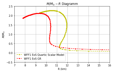
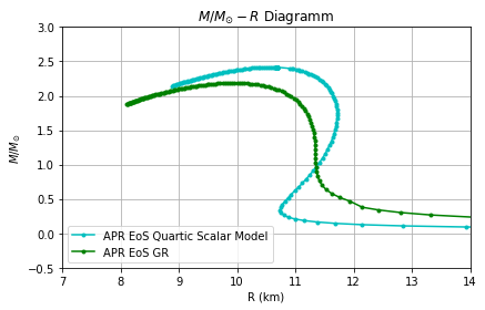
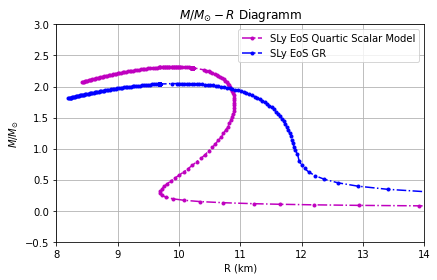
Let us now present the results of our numerical analysis and we also discuss the features of NSs when these are described by the quartic order scalar model. Let us start with the $M-R$ graphs, and in Figs. 1 we present the $M-R$ graphs for all the EoSs and we directly compare the quartic order scalar model results with the GR results, for $\xi\sim 11.455\times 10^{4}$. In the upper left we present the GR and quartic order scalar model $M-R$ graph for the WFF1 EoS, with the GR curve being red while the quartic order scalar model curve being yellow. In the upper right plot of Fig. 1 we present the APR $M-R$ graph for both GR (green curve) and the quartic order scalar model (cyan), while in the bottom plot of Fig. 1 we present the $M-R$ graph for the SLy EoS for GR (blue) and the quartic order scalar model (purple).

Clearly, the $M-R$ curves describe quite well the $M\sim 1.6M_{\odot}$ area, where the radius is expected to be constrained in the range $R=10.68^{+15}_{-0.04}$km Bauswein:2017vtn. More importantly, the WFF1 EoS in the context of GR, which was excluded by the GW170817 constraints Bauswein:2017vtn, in the case of the quartic order scalar model NS model, becomes compatible with the GW170817 constraints. In all the plots, the $y$-axis corresponds to $M/M_{\odot}$, where $M$ is the ADM mass, while the $x$-axis corresponds to the Jordan frame circumferential radius of the NS in kilometers. In Table 1 we collect all the maximum masses and the corresponding radii, for all the EoSs. The resulting picture is interesting since the only fundamental scalar experimentally verified in nature, the quartic order scalar model, leads to maximum NS radii which are higher but quite close to the corresponding GR limit, for all the EoSs studied in this paper. More importantly, for all the maximum radii static NS configurations appearing in Table 1, the corresponding radii are also compatible with the GW170817 constraint, which dictates that the radii corresponding to the maximum mass of a static NS must be larger than $R=9.6^{+0.14}_{-0.03}$km.

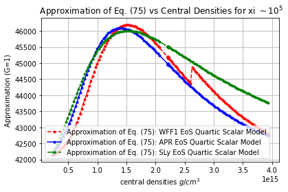
Furthermore, in Fig. 2 we present the values of the quantity $\xi^{2}\phi^{2}$ in the $y$-axis in Geometrized units, and in the $x$-axis the corresponding central densities in CGS units, in order to quantitatively verify the constraint (75), for $\xi\sim 11.455\times 10^{4}$. Obviously, the constraint (75) is well satisfied by our numerical results, for $\xi\sim 10^{4}$. In addition, we stress here that the constraint (63) is automatically satisfied for the values of $\xi$ we used in this article.

In this paper we studied the effects of a quartic order scalar model in static NSs, in the Einstein frame. We investigated quantitatively the properties of NSs when the quartic order scalar model potential is present. By using the approximation $\xi^{2}\phi^{2}\gg 1$ in the Jordan frame, which holds true for large $\xi$ values, we derived the Einstein frame TOV equations corresponding to a static spherically symmetric spacetime. With regard to the EoS, we used piecewise polytropic EoSs, with the central part being described by the SLy, APR and WFF1 EoS, which are well known successful EoSs. We numerically integrated the TOV equations using a double-shooting ”LSODA” python 3 based numerical code, and we extracted the NS masses and radii, as well as the values of the scalar field in the Einstein frame. With regard to the mass, we used the ADM mass in the Jordan frame, which is particularly useful for static spacetimes, and with regard to the radii, we converted the Einstein frame radii to their Jordan frame counterparts. We numerically solved the TOV equations for both the interior and the exterior of the NS, and the numerical study of the exterior was particularly demanding, needing a careful choice of the numerical infinity in order to optimize the central values of the scalar field and of the metric function that yield asymptotically at the numerical infinity, zero values for the scalar field and the metric function. The whole numerical study was performed for a large number of central densities. Using the masses and radii data, we constructed the $M-R$ graphs for the quartic order scalar model. For all the studied EoSs, the $M-R$ graphs were compatible with the observational constraints imposed by the GW170817 event which require the radius of a static $M\sim 1.6M_{\odot}$ neutron star to be larger than $R=10.68^{+15}_{-0.04}$km Bauswein:2017vtn and in addition the radius of a static neutron star corresponding to the maximum mass of the star to be larger than $R=9.6^{+0.14}_{-0.03}$km. Moreover, an important outcome of this work is the fact that although the WFF1 EoS was excluded for static neutron stars in the context of GR, for the quartic order scalar model neutron star model it provides realistic static NS configurations, which are compatible with both the aforementioned constraints of the GW170817 event Bauswein:2017vtn. We also carefully examined whether the initial approximation we made in the Jordan frame, namely $\xi^{2}\phi^{2}\gg 1$ holds true, and as we showed the approximation holds true. What now remains is to investigate how large are the baryon masses for such quartic order scalar model neutron stars, in order to understand the mass limit for which neutron stars will collapse to black holes. In the same line of research, it is important to calculate the causal mass limit for the present theory, with variable speed of sound, and investigate the qualitative behavior of the model. These two tasks may provide useful insights towards understanding how large can a neutron star mass be, and when do neutron stars can collapse to black holes. The latter can serve perhaps for a lower limit of astrophysical black holes masses, and may offer new insights to the difficult question, how small can astrophysical black holes masses be and how large a neutron star mass can be. Finally, the present work indicates that the quartic order scalar model predicts maximum radii for NS that are off the mass-gap region, thus it would be interesting to investigate whether string-corrected scalar field models, such as the Einstein-Gauss-Bonnet models Hwang:2005hb; Kanti:2015pda; DeLaurentis:2015fea; Yi:2018dhl; Kleihaus:2019rbg; Bakopoulos:2019tvc, may provide maximum masses inside the mass-gap region. We hope to address this issue in future works.

V.K. Oikonomou is indebted to N. Stergioulas and his MSc student Vaggelis Smyrniotis for the many hours spend on neutron star physics discussions and for sharing his professional knowledge on numerical integration of neutron stars in python. This work was supported by MINECO (Spain), project PID2019-104397GB-I00.

References

- (1) L. Tolos and L. Fabbietti, Prog. Part. Nucl. Phys. 112 (2020) 103770 doi:10.1016/j.ppnp.2020.103770 [arXiv:2002.09223 [nucl-ex]].
- (2) J. M. Lattimer, Ann. Rev. Nucl. Part. Sci. 62 (2012), 485-515 doi:10.1146/annurev-nucl-102711-095018 [arXiv:1305.3510 [nucl-th]].
- (3) A. W. Steiner and S. Gandolfi, Phys. Rev. Lett. 108 (2012), 081102 doi:10.1103/PhysRevLett.108.081102 [arXiv:1110.4142 [nucl-th]].
- (4) C. J. Horowitz, M. A. Perez-Garcia, D. K. Berry and J. Piekarewicz, Phys. Rev. C 72 (2005), 035801 doi:10.1103/PhysRevC.72.035801 [arXiv:nucl-th/0508044 [nucl-th]].
- (5) G. Watanabe, K. Iida and K. Sato, Nucl. Phys. A 676 (2000), 455-473 [erratum: Nucl. Phys. A 726 (2003), 357-365] doi:10.1016/S0375-9474(00)00197-4 [arXiv:astro-ph/0001273 [astro-ph]].
- (6) H. Shen, H. Toki, K. Oyamatsu and K. Sumiyoshi, Nucl. Phys. A 637 (1998), 435-450 doi:10.1016/S0375-9474(98)00236-X [arXiv:nucl-th/9805035 [nucl-th]].
- (7) J. Xu, L. W. Chen, B. A. Li and H. R. Ma, Astrophys. J. 697 (2009), 1549-1568 doi:10.1088/0004-637X/697/2/1549 [arXiv:0901.2309 [astro-ph.SR]].
- (8) K. Hebeler, J. M. Lattimer, C. J. Pethick and A. Schwenk, Astrophys. J. 773 (2013), 11 doi:10.1088/0004-637X/773/1/11 [arXiv:1303.4662 [astro-ph.SR]].
- (9) J. de Jesús Mendoza-Temis, M. R. Wu, G. Martínez-Pinedo, K. Langanke, A. Bauswein and H. T. Janka, Phys. Rev. C 92 (2015) no.5, 055805 doi:10.1103/PhysRevC.92.055805 [arXiv:1409.6135 [astro-ph.HE]].
- (10) W. C. G. Ho, K. G. Elshamouty, C. O. Heinke and A. Y. Potekhin, Phys. Rev. C 91 (2015) no.1, 015806 doi:10.1103/PhysRevC.91.015806 [arXiv:1412.7759 [astro-ph.HE]].
- (11) A. Kanakis-Pegios, P. S. Koliogiannis and C. C. Moustakidis, [arXiv:2012.09580 [astro-ph.HE]].
- (12) M. Buschmann, R. T. Co, C. Dessert and B. R. Safdi, Phys. Rev. Lett. 126 (2021) no.2, 021102 doi:10.1103/PhysRevLett.126.021102 [arXiv:1910.04164 [hep-ph]].
- (13) B. R. Safdi, Z. Sun and A. Y. Chen, Phys. Rev. D 99 (2019) no.12, 123021 doi:10.1103/PhysRevD.99.123021 [arXiv:1811.01020 [astro-ph.CO]].
- (14) A. Hook, Y. Kahn, B. R. Safdi and Z. Sun, Phys. Rev. Lett. 121 (2018) no.24, 241102 doi:10.1103/PhysRevLett.121.241102 [arXiv:1804.03145 [hep-ph]].
- (15) T. D. P. Edwards, B. J. Kavanagh, L. Visinelli and C. Weniger, [arXiv:2011.05378 [hep-ph]].
- (16) S. Nurmi, E. D. Schiappacasse and T. T. Yanagida, [arXiv:2102.05680 [hep-ph]].
- (17) A. V. Astashenok, S. Capozziello, S. D. Odintsov and V. K. Oikonomou, Phys. Lett. B 811 (2020), 135910 doi:10.1016/j.physletb.2020.135910 [arXiv:2008.10884 [gr-qc]].
- (18) S. Capozziello, M. De Laurentis, R. Farinelli and S. D. Odintsov, Phys. Rev. D 93 (2016) no.2, 023501 doi:10.1103/PhysRevD.93.023501 [arXiv:1509.04163 [gr-qc]].
- (19) A. V. Astashenok, S. Capozziello and S. D. Odintsov, JCAP 01 (2015), 001 doi:10.1088/1475-7516/2015/01/001 [arXiv:1408.3856 [gr-qc]].
- (20) A. V. Astashenok, S. Capozziello and S. D. Odintsov, Phys. Rev. D 89 (2014) no.10, 103509 doi:10.1103/PhysRevD.89.103509 [arXiv:1401.4546 [gr-qc]].
- (21) A. V. Astashenok, S. Capozziello and S. D. Odintsov, JCAP 12 (2013), 040 doi:10.1088/1475-7516/2013/12/040 [arXiv:1309.1978 [gr-qc]].
- (22) A. S. Arapoglu, C. Deliduman and K. Y. Eksi, JCAP 07 (2011), 020 doi:10.1088/1475-7516/2011/07/020 [arXiv:1003.3179 [gr-qc]].
- (23) A. V. Astashenok and S. D. Odintsov, Mon. Not. Roy. Astron. Soc. 498 (2020) no.3, 3616 doi:10.1093/mnras/staa2630 [arXiv:2008.11271 [gr-qc]].
- (24) A. Sedrakian, Phys. Rev. D 93 (2016) no.6, 065044 doi:10.1103/PhysRevD.93.065044 [arXiv:1512.07828 [astro-ph.HE]].
- (25) S. Khadkikar, A. R. Raduta, M. Oertel and A. Sedrakian, arXiv:2102.00988 [astro-ph.HE].
- (26) D. M. Sedrakian, M. V. Hayrapetyan and M. K. Shahabasyan, Astrophysics 49 (2006), 194-200 doi:10.1007/s10511-006-0020-4
- (27) A. Sedrakian, Phys. Rev. D 99 (2019) no.4, 043011 doi:10.1103/PhysRevD.99.043011 [arXiv:1810.00190 [astro-ph.HE]].
- (28) A. Bauswein, G. Guo, J. H. Lien, Y. H. Lin and M. R. Wu, [arXiv:2012.11908 [astro-ph.HE]].
- (29) S. Vretinaris, N. Stergioulas and A. Bauswein, Phys. Rev. D 101 (2020) no.8, 084039 doi:10.1103/PhysRevD.101.084039 [arXiv:1910.10856 [gr-qc]].
- (30) A. Bauswein, S. Blacker, V. Vijayan, N. Stergioulas, K. Chatziioannou, J. A. Clark, N. U. F. Bastian, D. B. Blaschke, M. Cierniak and T. Fischer, Phys. Rev. Lett. 125 (2020) no.14, 141103 doi:10.1103/PhysRevLett.125.141103 [arXiv:2004.00846 [astro-ph.HE]].
- (31) A. Bauswein, O. Just, H. T. Janka and N. Stergioulas, Astrophys. J. Lett. 850 (2017) no.2, L34 doi:10.3847/2041-8213/aa9994 [arXiv:1710.06843 [astro-ph.HE]].
- (32) E. R. Most, L. R. Weih, L. Rezzolla and J. Schaffner-Bielich, Phys. Rev. Lett. 120 (2018) no.26, 261103 doi:10.1103/PhysRevLett.120.261103 [arXiv:1803.00549 [gr-qc]].
- (33) L. Rezzolla, E. R. Most and L. R. Weih, Astrophys. J. Lett. 852 (2018) no.2, L25 doi:10.3847/2041-8213/aaa401 [arXiv:1711.00314 [astro-ph.HE]].
- (34) B. P. Abbott et al. [LIGO Scientific and Virgo], Phys. Rev. Lett. 119 (2017) no.16, 161101 doi:10.1103/PhysRevLett.119.161101 [arXiv:1710.05832 [gr-qc]].
- (35) S. D. Odintsov, V. K. Oikonomou and F. P. Fronimos, Nucl. Phys. B 958 (2020), 115135 doi:10.1016/j.nuclphysb.2020.115135 [arXiv:2003.13724 [gr-qc]].
- (36) V. K. Oikonomou and F. P. Fronimos, Class. Quant. Grav. 38 (2021) no.3, 035013 doi:10.1088/1361-6382/abce47 [arXiv:2006.05512 [gr-qc]].
- (37) R. Abbott et al. [LIGO Scientific and Virgo], Astrophys. J. Lett. 896 (2020) no.2, L44 doi:10.3847/2041-8213/ab960f [arXiv:2006.12611 [astro-ph.HE]].
- (38) P. Haensel, A. Y. Potekhin and D. G. Yakovlev, Astrophys. Space Sci. Libr. 326 (2007), pp.1-619 doi:10.1007/978-0-387-47301-7
- (39) J. L. Friedman and N. Stergioulas, doi:10.1017/CBO9780511977596
- (40) G. Baym, T. Hatsuda, T. Kojo, P. D. Powell, Y. Song and T. Takatsuka, Rept. Prog. Phys. 81 (2018) no.5, 056902 doi:10.1088/1361-6633/aaae14 [arXiv:1707.04966 [astro-ph.HE]].
- (41) J. M. Lattimer and M. Prakash, Science 304 (2004), 536-542 doi:10.1126/science.1090720 [arXiv:astro-ph/0405262 [astro-ph]].
- (42) G. J. Olmo, D. Rubiera-Garcia and A. Wojnar, Phys. Rept. 876 (2020), 1-75 doi:10.1016/j.physrep.2020.07.001 [arXiv:1912.05202 [gr-qc]].
- (43) A. Nathanail, E. R. Most and L. Rezzolla, Astrophys. J. Lett. 908 (2021) no.2, L28 doi:10.3847/2041-8213/abdfc6 [arXiv:2101.01735 [astro-ph.HE]].
- (44) S. Köppel, L. Bovard and L. Rezzolla, Astrophys. J. Lett. 872 (2019) no.1, L16 doi:10.3847/2041-8213/ab0210 [arXiv:1901.09977 [gr-qc]].
- (45) S. Nojiri, S. D. Odintsov and V. K. Oikonomou, Phys. Rept. 692 (2017) 1 doi:10.1016/j.physrep.2017.06.001 [arXiv:1705.11098 [gr-qc]].
- (46) S. Capozziello and M. De Laurentis, Phys. Rept. 509 (2011) 167 doi:10.1016/j.physrep.2011.09.003 [arXiv:1108.6266 [gr-qc]].
- (47) V. Faraoni and S. Capozziello, Fundam. Theor. Phys. 170 (2010). doi:10.1007/978-94-007-0165-6
- (48) S. Nojiri and S. D. Odintsov, eConf C 0602061 (2006) 06 [Int. J. Geom. Meth. Mod. Phys. 4 (2007) 115] doi:10.1142/S0219887807001928 [hep-th/0601213].
- (49) S. Nojiri and S. D. Odintsov, Phys. Rept. 505 (2011) 59 doi:10.1016/j.physrep.2011.04.001 [arXiv:1011.0544 [gr-qc]].
- (50) A. de la Cruz-Dombriz and D. Saez-Gomez, Entropy 14 (2012) 1717 doi:10.3390/e14091717 [arXiv:1207.2663 [gr-qc]].
- (51) G. J. Olmo, Int. J. Mod. Phys. D 20 (2011) 413 doi:10.1142/S0218271811018925 [arXiv:1101.3864 [gr-qc]].
- (52) Konstantinos Dimopoulos, Introduction to Cosmic Inflation and Dark Energy, (2021) CRC Press
- (53) A. V. Astashenok, S. Capozziello, S. D. Odintsov and V. K. Oikonomou, Phys. Lett. B 816 (2021), 136222 doi:10.1016/j.physletb.2021.136222 [arXiv:2103.04144 [gr-qc]].
- (54) N. Aghanim et al. [Planck], Astron. Astrophys. 641 (2020), A6 doi:10.1051/0004-6361/201833910 [arXiv:1807.06209 [astro-ph.CO]].
- (55) R. R. Caldwell, M. Kamionkowski and N. N. Weinberg, Phys. Rev. Lett. 91 (2003), 071301 doi:10.1103/PhysRevLett.91.071301 [arXiv:astro-ph/0302506 [astro-ph]].
- (56) F. Bezrukov and M. Shaposhnikov, Phys. Lett. B 734 (2014), 249-254 doi:10.1016/j.physletb.2014.05.074 [arXiv:1403.6078 [hep-ph]].
- (57) J. Garcia-Bellido, J. Rubio, M. Shaposhnikov and D. Zenhausern, Phys. Rev. D 84 (2011), 123504 doi:10.1103/PhysRevD.84.123504 [arXiv:1107.2163 [hep-ph]].
- (58) F. Bezrukov, A. Magnin, M. Shaposhnikov and S. Sibiryakov, JHEP 01 (2011), 016 doi:10.1007/JHEP01(2011)016 [arXiv:1008.5157 [hep-ph]].
- (59) F. L. Bezrukov and M. Shaposhnikov, Phys. Lett. B 659 (2008), 703-706 doi:10.1016/j.physletb.2007.11.072 [arXiv:0710.3755 [hep-th]].
- (60) S. S. Mishra, V. Sahni and A. V. Toporensky, Phys. Rev. D 98 (2018) no.8, 083538 doi:10.1103/PhysRevD.98.083538 [arXiv:1801.04948 [gr-qc]].
- (61) C. F. Steinwachs and A. Y. Kamenshchik, AIP Conf. Proc. 1514 (2013) no.1, 161-164 doi:10.1063/1.4791748 [arXiv:1301.5543 [gr-qc]].
- (62) J. Rubio, Front. Astron. Space Sci. 5 (2019), 50 doi:10.3389/fspas.2018.00050 [arXiv:1807.02376 [hep-ph]].
- (63) D. I. Kaiser, Phys. Rev. D 52 (1995), 4295-4306 doi:10.1103/PhysRevD.52.4295 [arXiv:astro-ph/9408044 [astro-ph]].
- (64) A. Gundhi and C. F. Steinwachs, Nucl. Phys. B 954 (2020), 114989 doi:10.1016/j.nuclphysb.2020.114989 [arXiv:1810.10546 [hep-th]].
- (65) J. L. Cervantes-Cota and H. Dehnen, Nucl. Phys. B 442 (1995), 391-412 doi:10.1016/0550-3213(95)00128-X [arXiv:astro-ph/9505069 [astro-ph]].
- (66) K. Kamada, T. Kobayashi, T. Takahashi, M. Yamaguchi and J. Yokoyama, Phys. Rev. D 86 (2012), 023504 doi:10.1103/PhysRevD.86.023504 [arXiv:1203.4059 [hep-ph]].
- (67) S. Schlogel, M. Rinaldi, F. Staelens and A. Fuzfa, Phys. Rev. D 90 (2014) no.4, 044056 doi:10.1103/PhysRevD.90.044056 [arXiv:1405.5476 [gr-qc]].
- (68) A. Füzfa, M. Rinaldi and S. Schlögel, Phys. Rev. Lett. 111 (2013) no.12, 121103 doi:10.1103/PhysRevLett.111.121103 [arXiv:1305.2640 [gr-qc]].
- (69) Y. Akrami et al. [Planck], Astron. Astrophys. 641 (2020), A10 doi:10.1051/0004-6361/201833887 [arXiv:1807.06211 [astro-ph.CO]].
- (70) P. Pani and E. Berti, Phys. Rev. D 90 (2014) no.2, 024025 doi:10.1103/PhysRevD.90.024025 [arXiv:1405.4547 [gr-qc]].
- (71) K. V. Staykov, D. D. Doneva, S. S. Yazadjiev and K. D. Kokkotas, JCAP 10 (2014), 006 doi:10.1088/1475-7516/2014/10/006 [arXiv:1407.2180 [gr-qc]].
- (72) M. Horbatsch, H. O. Silva, D. Gerosa, P. Pani, E. Berti, L. Gualtieri and U. Sperhake, Class. Quant. Grav. 32 (2015) no.20, 204001 doi:10.1088/0264-9381/32/20/204001 [arXiv:1505.07462 [gr-qc]].
- (73) H. O. Silva, C. F. B. Macedo, E. Berti and L. C. B. Crispino, Class. Quant. Grav. 32 (2015), 145008 doi:10.1088/0264-9381/32/14/145008 [arXiv:1411.6286 [gr-qc]].
- (74) D. D. Doneva, S. S. Yazadjiev, N. Stergioulas and K. D. Kokkotas, Phys. Rev. D 88 (2013) no.8, 084060 doi:10.1103/PhysRevD.88.084060 [arXiv:1309.0605 [gr-qc]].
- (75) R. Xu, Y. Gao and L. Shao, Phys. Rev. D 102 (2020) no.6, 064057 doi:10.1103/PhysRevD.102.064057 [arXiv:2007.10080 [gr-qc]].
- (76) M. Salgado, D. Sudarsky and U. Nucamendi, Phys. Rev. D 58 (1998), 124003 doi:10.1103/PhysRevD.58.124003 [arXiv:gr-qc/9806070 [gr-qc]].
- (77) M. Shibata, K. Taniguchi, H. Okawa and A. Buonanno, Phys. Rev. D 89 (2014) no.8, 084005 doi:10.1103/PhysRevD.89.084005 [arXiv:1310.0627 [gr-qc]].
- (78) A. Savaş Arapoğlu, K. Yavuz Ekşi and A. Emrah Yükselci, Phys. Rev. D 99 (2019) no.6, 064055 doi:10.1103/PhysRevD.99.064055 [arXiv:1903.00391 [gr-qc]].
- (79) F. M. Ramazanoğlu and F. Pretorius, Phys. Rev. D 93 (2016) no.6, 064005 doi:10.1103/PhysRevD.93.064005 [arXiv:1601.07475 [gr-qc]].
- (80) Z. Altaha Motahar, J. L. Blázquez-Salcedo, D. D. Doneva, J. Kunz and S. S. Yazadjiev, Phys. Rev. D 99 (2019) no.10, 104006 doi:10.1103/PhysRevD.99.104006 [arXiv:1902.01277 [gr-qc]].
- (81) X. Y. Chew, V. Dzhunushaliev, V. Folomeev, B. Kleihaus and J. Kunz, Phys. Rev. D 100 (2019) no.4, 044019 doi:10.1103/PhysRevD.100.044019 [arXiv:1906.08742 [gr-qc]].
- (82) J. L. Blázquez-Salcedo, F. Scen Khoo and J. Kunz, EPL 130 (2020) no.5, 50002 doi:10.1209/0295-5075/130/50002 [arXiv:2001.09117 [gr-qc]].
- (83) Z. Altaha Motahar, J. L. Blázquez-Salcedo, B. Kleihaus and J. Kunz, Phys. Rev. D 96 (2017) no.6, 064046 doi:10.1103/PhysRevD.96.064046 [arXiv:1707.05280 [gr-qc]].
- (84) S. D. Odintsov and V. K. Oikonomou, Phys. Dark Univ. 32 (2021), 100805 doi:10.1016/j.dark.2021.100805 [arXiv:2103.07725 [gr-qc]].
- (85) J. S. Read, B. D. Lackey, B. J. Owen and J. L. Friedman, Phys. Rev. D 79 (2009), 124032
- (86) J. S. Read, C. Markakis, M. Shibata, K. Uryu, J. D. E. Creighton and J. L. Friedman, Phys. Rev. D 79 (2009), 124033
- (87) A. Komar, Phys. Rev. 113 (1959), 934-936 doi:10.1103/PhysRev.113.934
- (88) R. Arnowitt, S. Deser and C. W. Misner, Phys. Rev. 118 (1960), 1100-1104 doi:10.1103/PhysRev.118.1100
- (89) M. Shibata and K. Kawaguchi, Phys. Rev. D 87 (2013) no.10, 104031 doi:10.1103/PhysRevD.87.104031
- (90) Nikolaos Stergioulas, https://github.com/niksterg
- (91) Valerio Faraoni, Cosmology in Scalar-Tensor Gravity, Springer 2004
- (92) V. Faraoni, Galaxies 1 (2013) no.2, 96-106
- (93) M. Buck, M. Fairbairn and M. Sakellariadou, Phys. Rev. D 82 (2010), 043509
- (94) V. Faraoni, E. Gunzig and P. Nardone, Fund. Cosmic Phys. 20 (1999) 121 [gr-qc/9811047].
- (95) R. B. Wiringa, V. Fiks and A. Fabrocini, Phys. Rev. C 38 (1988), 1010-1037 doi:10.1103/PhysRevC.38.1010
- (96) F. Douchin and P. Haensel, Astron. Astrophys. 380 (2001), 151 doi:10.1051/0004-6361:20011402 [arXiv:astro-ph/0111092 [astro-ph]].
- (97) A. Akmal, V. R. Pandharipande and D. G. Ravenhall, Phys. Rev. C 58 (1998), 1804-1828 doi:10.1103/PhysRevC.58.1804 [arXiv:nucl-th/9804027 [nucl-th]].
- (98) S.D. Odintsov, I.L. Shapiro, Effective action in quantum gravity I.L. Buchbinder, Published in Bristol, UK: IOP (1992) 413 p
- (99) T. Muta, S.D. Odintsov, Mod.Phys.Lett. A6 (1991) 3641-3646 DOI: 10.1142/S0217732391004206 a
- (100) I. L. Buchbinder and S. D. Odintsov, Lett. Nuovo Cim. 42 (1985) 379. doi:10.1007/BF02747058 ))
- (101) J. c. Hwang and H. Noh, Phys. Rev. D 71 (2005) 063536 doi:10.1103/PhysRevD.71.063536 [gr-qc/0412126].
- (102) P. Kanti, R. Gannouji and N. Dadhich, Phys. Rev. D 92 (2015) no.4, 041302 doi:10.1103/PhysRevD.92.041302 [arXiv:1503.01579 [hep-th]].
- (103) M. De Laurentis, M. Paolella and S. Capozziello, Phys. Rev. D 91 (2015) no.8, 083531 doi:10.1103/PhysRevD.91.083531 [arXiv:1503.04659 [gr-qc]].
- (104) Z. Yi and Y. Gong, Universe 5 (2019) no.9, 200 doi:10.3390/universe5090200 [arXiv:1811.01625 [gr-qc]].
- (105) B. Kleihaus, J. Kunz and P. Kanti, arXiv:1910.02121 [gr-qc].
- (106) A. Bakopoulos, P. Kanti and N. Pappas, Phys. Rev. D 101 (2020) no.4, 044026 doi:10.1103/PhysRevD.101.044026 [arXiv:1910.14637 [hep-th]].