Deep Reinforcement Learning Powered IRS-Assisted Downlink NOMA
Abstract
In this work, we examine an intelligent reflecting surface (IRS) assisted downlink non-orthogonal multiple access (NOMA) scenario with the aim of maximizing the sum rate of users. The optimization problem at the IRS is quite complicated, and non-convex, since it requires the tuning of the phase shift reflection matrix. Driven by the rising deployment of deep reinforcement learning (DRL) techniques that are capable of coping with solving non-convex optimization problems, we employ DRL to predict and optimally tune the IRS phase shift matrices. Simulation results reveal that IRS assisted NOMA based on our utilized DRL scheme achieves high sum rate compared to OMA based one, and as the transmit power increases, the capability of serving more users increases. Furthermore, results show that imperfect successive interference cancellation (SIC) has a deleterious impact on the data rate of users performing SIC. As the imperfection increases by ten times, the rate decreases by more than 10%.
Index Terms:
Intelligent Reflecting Surfaces (IRS), Non-Orthogonal Multiple Access (NOMA), Deep Reinforcement learning (DRL), 5G and beyond, 6G, Phase shift design.I Introduction
With the increasing progressions in the wireless communications, future communication systems are favorable to support higher data rates, higher spectral efficiencies, reduced latencies, wider coverage areas and massive number of connections, among other features.
As wireless technologies have grown exponentially over the last few decades, wireless systems are promising to meet the demand for the enormous number of connections. The next generation networks will be an end-to-end ecosystem to enable a fully connected and sustainable community. The main purpose of these networks is to provide seamless and ubiquitous communications for users with a higher throughput, low latency, low energy consumption and support the escalation in mobile data consumption for hundreds of thousands of connections. As 5G networks are being deployed, technologies for 6G networks are being researched and examined to attain more reliable and faster communication systems [1].
Among these technologies, are the intelligent reflecting surfaces (IRS)s, which regulate the wireless environment to boost the energy and spectral efficiencies. IRS consists of a huge number of passive elements or IRS units, each unit can passively reflect the incident electromagnetic wave signal and modify it in terms of phase, frequency, amplitude or polarization. Most of the research papers in the literature are considering passive IRS where only a phase shift to the incident signal is applied. Thus, the IRS will not consume any transmit power. Consequently, the IRS optimization problem is focused on the phase-shift matrix [2]. Further, the IRS can aid the transmissions among the transmitters and receivers, especially where there is no line of sight (LoS) between the transmitting antenna and the receiving antenna, or if the direct link suffers from shadowing and deep fading rendering the quality of the channel for direct communications unreliable [3]. Compared to decode and forward and amplify and forward, IRS demands less energy and power consumption because of its passive features. Hence, IRS is anticipated to be a promising solution for future 5G / 6G communication systems [4]. IRS can be related to technologies such as massive or large multiple input multiple output (M-MIMO) antenna networks since it utilizes large number of antennas to increase the energy and spectrum efficiency. Thus, IRS is considered a potential component in 6G networks, which is analogous to M-MIMO potential in 5G networks. Nonetheless, the difference is that the IRS regulates the propagation in the wireless environment.
Non-orthogonal multiple access (NOMA) is a vital component in 5G wireless communication systems and beyond because of the high spectrum efficiency it provides in addition to its support for massive connectivity. In the previous cellular systems, many multiple access technologies were adopted such as the time division multiple access (TDMA), frequency division multiple access (FDMA), spatial division multiple access (SDMA) and orthogonal frequency division multiple access (OFDMA). Based on their design, these technologies are considered as orthogonal multiple access (OMA) techniques, since the wireless resources are allocated to multiple users orthogonally. The users are separated in the chosen access domain whether it is in frequency, time, or space. If orthogonality is violated, the users will suffer from interference and quality of communications links will degrade leading to loss of information and/or inefficient resources utilization. Nonetheless, OMA schemes cannot satisfy the requirements for future communication systems which causes the need for NOMA [5]. NOMA achieves high sum rate capacity as compared to the traditional orthogonal multiple access (OMA) techniques. The reason is that it enables multiple users to transmit simultaneously in the same set of shared resources. This results in an interference, but NOMA utilizes a method called successive interference cancellation (SIC) to eliminate the resulting interference.
I-A Related Work
Many research studies related to IRS in 5G and 6G communication networks are being conducted. Some of these studies inspected IRS for OMA schemes such as in [6] - [10], but these studies did not include NOMA in their scenarios. However, several recent research studies started investigating IRS for NOMA communication. The authors in [11] examined an uplink scenario for IRS NOMA and they maximized the sum rate for all users taking into consideration the power constraint for each user. They solved the non-convex problem using semi-definite relaxation which is a mathematical method and provides near-optimal solution. In [12], the authors proposed a simple design for the IRS assisted NOMA system. First they utilized spatial division multiple access on the base station (BS) side for orthogonal beams generation. This is done by making use of the spatial directions of the channels of the nearby users. Then the authors employed IRS aided NOMA to serve the additional users on the cell edge. They demonstrated the performance of the IRS-NOMA system by providing analytical results. The authors in [13] inspected secure communication transmission in IRS assisted NOMA system for a practical eavesdropper scenario having imperfect channel state information. They proposed a joint IRS phase shift and transmit beamforming scheme to ensure secure transmission via IRS. Moreover, they used the alternating optimization algorithm which is a mathematical method to find out stationary point solutions. Further, in [14] IRS assisted downlink NOMA system was considered with the aim of enhancing the performance of the rate and maximizing the signal to interference plus noise ratio (SINR). The authors achieved this by jointly optimizing the phase shift at the IRS and the transmit beamforming at the BS. They used efficient mathematical method based on semi-definite relaxation and block coordinated decent techniques. mmWave technology was included in the IRS NOMA scenario in [15], where the authors inspected the downlink scenario of IRS mmWave NOMA, and the formulated problem included joint optimization of the passive and active beamforming as well as power allocation with the aim of enhancing the performance of the system. To solve the problem, the authors used a mathematical method based on an iterative algorithm utilizing successive convex approximation and alternating optimization.
Nonetheless, the above studies [11] - [15] assumed that the channels between the IRS and users are known. Such assumption contradicts the practical case, where IRSs are passive elements incapable of estimating channels. In the case where part of the channels are unknown, the use of machine learning techniques can add value to the problem.
I-B Contributions
In our research work, we address the aforementioned gap in surveyed literature by leveraging reinforcement learning (RL); in particular, deep reinforcement learning (DRL), to optimize the sum rate of a NOMA downlink system utilizing IRS under the assumption of unknown channel states information between the IRS and users. In particular, we exploit Deep Deterministic Policy Gradient (DDPG) due to its suitability for our scenario because the problem is non-convex, the objective function is non-convex and the unit modulus constraints are fundamentally non-convex. Therefore, it is an NP-hard problem [8], [16]. The major challenge presents in the constant modulus constraint of the phase shift since the IRS can reflect the signal without amplifying it. Hence, it is not easy to obtain an optimal solution in closed form. The use of DDPG is very efficient when coping with intractable problems, it will remove the need for gathering a large dataset for training. DDPG method is anticipated to provide a solid and robust performance.
Our contributions in this work can be summarized as follows:
- •
First, we formulate the IRS NOMA downlink phase shift optimization problem with the objective of maximizing the sum-rate for NOMA users taking into consideration that the instantaneous channel states information between the IRS and users are unknown.
- •
Second, we incorporate imperfect interference cancellation in practical NOMA within our system model formulation.
- •
Third, DDPG based solution is proposed for predicting the best phase shift matrix in which the IRS learns the best way for reflecting the incident signals by modifying the phase.
- •
Fourth, numerical results reveal the effectiveness of the DDPG algorithm, since the sum rate value for the DDPG based IRS assisted NOMA system outperforms OMA based systems with minimum training overhead.
I-C Paper organization
The rest of the paper is structured as follows. Section II outlines the system and channel model. Section III explains the DDPG-based phase control for IRS. Section IV presents the numerical results, and Section V concludes the paper.
II System Model
We consider the downlink of an IRS assisted NOMA system with users as shown in Fig. 1. Without loss of generality, the users are ordered according to their distance from the IRS such that user is the farthest user from the IRS and user is the nearest user to the IRS. Consequently, the users can be considered as ordered based on the expected value of their channel gains assuming . All users as well as the BS are assumed to have a single antenna each. It is assumed that there is no direct line of sight (LOS) link between the users and the BS. Thus, the communication between the BS and users is performed through the IRS which is deployed with reflecting elements, where and represent the number of passive elements in the IRS in every row and column, respectively.
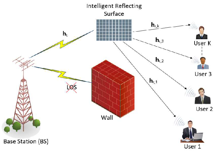
The transmitted signal at the BS is
| (1) |
where represents the signal for user with unit power (i.e., , , where denotes the expectation). The power allocated to each user is , where is the vector of coefficients of the users’ power allocated such that and is the BS total transmit power. The power allocated for users is fixed and it satisfies the relationship: . When allocating power to users, we will take into consideration the following conditions , , and so on.
The received signal for user k can be written as:
| (2) | ||||
where is the channel between the BS and the IRS, and is the channel between the IRS and users. Both channels follow the Rician fading model:
| (3) |
| (4) |
where is the rician factor of , and are the LoS component and non-LoS (NLoS) component, respectively. Similarly, is the rician factor of , and are the LoS component and non-LoS (NLoS) component, respectively. The phase shift reflection matrix is represented by , and satisfies the constant modulus constraint , , because the IRS reflects the signal without amplifying it, where denotes a diagonal matrix. Further, the phase shift of the passive reflecting element is denoted by , where the value of is between and , and represents the additive white Gaussian noise (AWGN).
Hence, the received SINR at user can be represented by the following equation:
| (5) |
when , the term .
Furthermore, the data rate of user is represented by:
| (6) |
Our objective in this study is to maximize the sum-rate of all users where:
| (7) |
Therefore, the formulated problem at the IRS is to obtain the phase shift reflection matrix that maximizes for users.
| (8) | ||||
The above equation (8) is valid for perfect successive interference cancellation (SIC) which is the ideal case, where the interference from the far users is assumed to be perfectly eliminated at the near users receiver. In this case near users have perfect knowledge of the far users’ data signal. Nonetheless, in the case of imperfect SIC, the interference of the far users is not perfectly removed at the near users receiver. In this case, the data signal of the far user is not perfectly known at the near user due to distortion caused by fading and AWGN which is more realistic practically. Thus, the received SINR in (5) at user can be rewritten as:
| (9) |
when = 1, the term . The term epsilon () represents the fraction of the residual interference leftover due to imperfect SIC.
Accordingly, the optimization problem in (8) becomes
| (10) | ||||
II-A Upperbound on Performance
To measure the performance of the DDPG algorithm and to verify that our sum-rate values approach the upperbound, an exhaustive search method is used to search for the optimum phase shift matrix that results in the maximum sum-rate as shown in Algorithm 1. Further, to avoid the huge complexity of the exhaustive search scheme, we will consider a limited number of IRS reflecting elements as a case proof that our DDPG algorithm can track the upperbound. For every IRS element we will consider the phases between 0 and with a step size of 16, this will give us combinations of phase shift matrices. Then we will calculate the sum-rates accordingly for users.
II-B OMA Baseline Scheme
The signal model for OMA is assumed such that the resources (frequency / time) are divided equally between the users. This enables OMA users to receive the signal with free interference, whereas the merit of NOMA is the simultaneous transmission and the interference can be controlled. However, to serve K OMA users, FDMA / TDMA requires time slots. The first user will use the first frequency/time slot, the second user will use the second frequency/time slot, and user will use the frequency/time slot accordingly.
The transmitted signal by the BS is given by:
| (11) |
The received signal at the user side can be expressed as:
| (12) |
Hence, the received SNR at user k can be represented as:
| (13) |
Further, data rate of user k is represented by:
| (14) |
Therefore, the sum-rate of OMA can be expressed as:
| (15) |
| (16) |
III Proposed DRL-Based Phase Control for IRS
III-A Overview on DRL method:
Reinforcement Learning (RL) method is a field of machine learning that allows the agent in an interactive environment to learn by trial and error relying on a feedback from its own experiences. The model in Fig. 2 demonstrates the basic concept of the RL. Further, the fundamental factors that characterize the RL problem are the agent, environment, state, reward, policy, and value. The environment is the physical surrounding where the agent operates, the state is the agent’s current status, the reward is the feedback the agent experience from the environment, the policy is the process of mapping the state of the agent to actions, and the value is the agent’s future reward that it receives when taking action in a specific state. The agent at time gets state from the environment and selects action based on policy . After selecting the action the state changes from to and generate reward . The objective of RL is to maximize the total reward, the reward is the performance measure of a specific action during the current state. RL models the interaction between the agent and the environment as Markov’s decision process (MDP). Many RL algorithms use dynamic programming methods, but the prime difference between RL algorithms and dynamic programming is that RL algorithms don’t assume the awareness of a specific MDP’s mathematical model. Further, RL algorithms are aimed for large MDPs in which specific procedures become impracticable [17].

Q-learning (QL) is a model-free RL method since it does not require a model, it obtains the best action under the current state, where "Q" denotes the quality. Further, it is an off-policy algorithm since QL learns actions that are outside the current policy so it may take actions that are random and therefore the policy is not needed here. When the agent interacts with the environment and needs to update the action-state pairs in the Q-table, it has two choices, either to explore or exploit. Exploration is to explore the environment in order to obtain information and knowledge about it, in this case the agent acts randomly. Whereas exploitation is to exploit the available "already known" information about the environment so as to maximize the reward. Precisely, QL selects the optimal policy in order to maximize the total reward.
The trade-off between exploration and exploitation is balanced by using a specific parameter which can be set based on how often we want to exploit or explore. Moreover, QL is based on the concept of a Q-function, which is a function of states and actions. The Q-function measures the expected discounted sum of rewards or the return achieved from selecting action in a state based on policy . It evaluates how good a particular action is, for a given state. The optimal Q-value is defined as the maximum return achieved from a given state and action while obeying the optimal policy. In order to update the Q-value for any action we use the Bellman equation. It provides us the best reward and the optimal policy to achieve this reward. It means that the maximum value of the return from the action and state is equal to the expectation of the current maximum possible reward plus the maximum possible long-term reward achieved from the next state s’ discounted by which is the discount factor, and the equation is expressed as:
| (17) |
where denotes the expectation. The updates will occur after each action and it will end when the episode finishes. In order to converge and learn optimal values, the agent needs to learn and explore many episodes. Furthermore, there are three important steps in the update, the first step is that the agent will take action for each state and receive a reward. The second step is that the agent will either select the action by checking the highest value in the Q-table or by random . The third step is to update the Q-values employing the following formula:
| (18) |
The step size is adjusted using the learning rate which measures the acceptance of the new value compared to the old one [17].

Deep Q-Learning (DQL) uses neural network that approximates the Q-function. Fig. 3 shows a comparison between QL and DQL, instead of calculating Q-values immediately for each action and state via iterations, we will utilize a function approximator for estimating Q-values for each possible action. To perform this we need to employ neural networks (NN). The NN accepts states as input from the environment and generates the estimated Q-values for every action the agent can select. Furthermore, in many problems in DQL it is not practical to represent the Q-function based on and only, the reason is that we will train the neural network (NN) with parameters to evaluate the Q-values such that .
| (19) |
where is the cumulative expected reward. The aim of the DQN is to maximize the value of the Q-function in (19) by DNN training. The optimal Q-value is obtained from the Bellman equation. At this stage, we can calculate the loss by comparing the Q-value for a given state-action pair to the target value which is the right hand side of the Bellman equation expression which gives us the below expressions:
| (20) |
| (21) |
Next the NN will update its weight values in the policy network based on the gradient descent and back propagation algorithms. We will keep repeating this process time after time for many episodes until we sufficiently minimize the loss [17].
Policy gradient (PG) is on-policy, model-free RL method, used for continuous action space. The PG agent is a RL agent which is policy-based, it aims directly to maximize the expected reward by obtaining a parametrized policy that generates a trajectory , where the trajectory represents the states, actions and rewards i.e. . In other words, we need to find out the parameters that maximizes , where represents the weights of the neural networks.
| (22) |
where denotes the total reward for a specified trajectory . A well known approach in machine learning to solve the maximization problem is the gradient descent or ascent to step through the parameters. By using the gradient ascent we get the following equation:
| (23) |
where represents the learning rate.
| (24) |
By reformulating the gradient we get:
,
The theory of the policy gradient states that the derivative of the expectation of the reward is equivalent to the expectation of the reward times the gradient of the log policy :
| (25) |
Therefore, the policy training is demonstrated as a gradient ascent process:
| (26) |
where is the Q-value for the trajectory , and policy . Throughout the training, the PG agent estimates the probability of selecting each action and chooses actions by random depending on the probability distribution. Before it learns from experience and updates the policy parameters, the PG agent performs a full training episode utilizing the existing policy. The disadvantage of PG method is that the network policy is updated after the completion of the episode only. This slackens the convergence rate [17].
III-B DDPG-based IRS phase control method
We propose a DDPG-based IRS phase control method considering the optimization problem in (8). Deep Q-Networks are not suitable because they deal with discrete time spaces only. Moreover, the convergence of the policy gradient (PG) algorithm is not sufficient in the context of wireless communication. DDPG merges the Q-networks and the PG scheme as shown in Fig. 4, and overcomes the disadvantages of both algorithms[17].

DDPG is a model-free reinforcement learning technique which combines the advantages of policy gradients and Q-learning. DDPG uses the Bellman equation and the off-policy data to learn the Q-function, and then uses the Q-function to learn the policy. DDPG consists of four neural networks (see Fig. 5); one for actor network, one for critic network, one for target actor network, and one for target critic network, which ensures the stability. The optimization problem in (8) can be solved using DDPG by learning the policy.
The actor network is a policy network that accepts state as input and generates the precise action continuously. In deep Q-networks the optimal action is obtained by calculating the argmax over all the Q-values for a finite number of discrete actions. In DDPG the actor network performs the same but for continuous action spaces, it generates the actions directly by taking the argmax, and selects actions from a continuous action settings , where is the policy, denotes the states, and denotes the parameters of the deterministic policy network (DPN). Thus, the actor is a DPN that calculates the action directly, rather than generating the probability distributions over all actions. The critic network accepts states and actions as input and generates the Q-value, so it is considered as the Q-value network , where represents the parameters of the Q-network. The critic network evaluates the performance of the selected action. Therefore, DDPG is an enhancement for the actor-critic vanilla network, its aim is to maximize the Q-value which is the output, and it can only be utilized for environments having continuous action settings. The optimal action is expressed as:
| (27) |
where is the optimal Q-value function. Further, to maximize the Q-value a replay memory is utilized to minimize the correlation of various training samples. This is significant for the algorithm behavior in order to be stable. The replay memory needs to be adequately large to include a broad range of previous experiences. Moreover, DDPG makes use of target networks to increase the stability during the training.
A copy from the actor and critic network are formed to find out the Q-value for the next state i.e. and . Based on the main networks, the weights of these target networks are updated periodically. In deep Q-networks, the weight of the main network is copied periodically to the target network and this called "hard update", whereas in DDPG "soft update" is performed where a only fraction of the weights of the main network are transferred to the target network as expressed below:
| (28) | |||
| (29) |

where . Soft updates are significant in order to accelerate the convergence of the Actor-Critic process since it stabilizes learning. The main networks which are copied are called evaluation networks. The target networks and the evaluation networks have the same structure but the difference is in parameters. The target networks are delayed networks compared to the main networks [17].
III-C RL System Mapping
The first step in solving a problem using RL is to map the problem into the key components of an RL system; namely, state-space, action space, and reward function. In the following, we discuss this mapping as well as the general behaviour of the RL method using DDPG.
III-C1 State-space
The state space of the DDPG agent at timestep can be defined as follows
| (30) |
where represents the channel gain between the source and IRS, is the last phase action taken by IRS, and is the estimated SINR values of the users based on their data rates for that action (i.e., ).
III-C2 Action-space
The action space definition is defined by the policy function as follows
| (31) |
where is the policy function and is parameters (i.e., weights of neural network), and is the Ornstein-Uhlenbeck (OU) process-based action noise [18]. Final output is an array that defines the phase of each element in the IRS.
III-C3 Reward function
The reward function is defined based on the current channel capacity and the maximum capacity ever reached as follows:
| (32) |
where is the actual sum-rate of the users, while is the maximum sum-rate achieved.
III-C4 Exploration vs. Exploitation
Since the action space of the DDPG is continuous, the exploration of action space is handled with noise generated by the OU process. OU process samples noise from a correlated normal distribution.
III-C5 DDPG Algorithm
As shown in Algorithm 2, we begin initializing the replay buffer of the agent with transaction capacity in step 1. In step 2, we initialize the weights of actor and critic networks for the agent. The target networks are initialized by copying the same weights in step 3. From step 4 to 13, represents each iteration (i.e., timestep ). In each iteration (i.e., timestep ), we observe the state s for the agent (IRS), determine an action (i.e., phase value) with exploration noise based on OU process in step 5. After the agent determined and executed the action, a reward is received and new state is observed, and transactions are stored in respective replay memories in steps 6 and 7. A random mini-batch of transitions are sampled in step 8. Using the Bellman equation, the actors and critic networks’ targets are computed in step 9. The critic network weights are updated by minimizing the loss using computed targets in step 10. The actor network weights are updated for the sampled policy gradient in step 11. Finally, the agent’s target networks are updated using the update rate () for stability in step 12.
III-C6 Neural Network Architecture
DDPG agent’s architecture consists of neural networks including actor and critic networks and target actor and critic for stability. Both actor and critic networks consist of hidden layers, with hidden nodes in each layer. The actor-network input has the size of , and output is , thanks to the continuous definition of DDPG. As can be seen from DDPG agents’ structure, it allows scalability to a much larger extent with linearly increasing complexity.
III-D Discussion on Complexity
To reveal the value of using DDPG, we provide a quick quantitative analysis of the exhaustive search algorithm complexity, versus the complexity, of the proposed DDPG based algorithm. The complexities can be easily deduced from the description of the algorithms given in Algorithm 1 and Algorithm 2. For exhaustive search asssuming users, IRS elements and phase change steps, we can write the complexity as
| (33) |
For the DDPG based system, the complexity for the trained network (steady state complexity) depends mainly on the forward network architecture (Actor Network). Assume the number of states (size of actor network input) is , number of hidden layers is , number of neurons in each hidden layer is , number of actions (i.e., phase of each IRS element) which is size of the output layer is , and the DDPG algorithm will always provide the action of the highest reward for the distinct actions as output. Therefore, the complexity of the DDPG can be written as
| (34) |
Thus, the complexity of DDPG is much lower than that of the exhaustive search as the number of users or the number of IRS elements increases.
IV Numerical Results
In this section, we first measured the performance of the DDPG algorithm to make sure that the sum-rate values calculated are close to the upperbound. By using the exhaustive search algorithm we calculated the maximum sum-rate by obtaining the optimum phase shift matrix and assuming that the channel is known. The exhaustive search scheme is very complex, so the number of IRS reflecting element used is = 4 rather than = 16. This is to verify that our DDPG algorithm can approach the upperbound. For each element we considered the phases between 0 and with a step size of 16. Thus, the total number of combinations of phase shift matrices is . The sum-rates are calculated for 16 users and for monte-carlo simulations equal to 1000. Fig. 6 reveals that NOMA sum-rate generated by the DDPG algorithm approaches the upperbound and it is close to optimal. The complexity of the exhaustive search algorithm can be calculated as 1000 x which is equal to iterations with elapsed time equal to 12.51 hours.


Moreover, the result in Fig. 7 verifies the convergence of our DRL algorithm. It shows the average NOMA rate verses the iteration plots. The average rate is increasing with time. This means that the training process is conducted successfully. Further, the simulation results below reveal the performance of our DRL based IRS NOMA system with IRS reflecting elements . The default parameters used in the simulation are shown in Table I. The number of of users is , the number of BS antennas is , the number of antennas per each user is , the distance between the BS and the IRS is 50 m and the distances between the IRS and the users are randomly generated between 200 and 1500 m. The channel between the BS and the IRS and the channel between the IRS and users follow the rician fading model with rician factor K1 = K2 = 10. However, the channel between the BS and the IRS is assumed to be perfectly estimated, whereas the channels between the IRS and users are assumed to be unknown. The bandwidth is 10 MHz, the BS transmit power Pt is 40 dBm, and the noise power spectral density equals -174 dBm/Hz. Simulation results are generated using monte-carlo runs.

| Simulation Parameters | Values |
| Number of Users (K) | 32 |
| Number of Reflecting Elements (M) | 16 |
| Number of BS antennas | 1 |
| Number of antennas per user | 1 |
| Distance between BS and IRS | 50 |
| Distance between the IRS and the users | 200 - 1500 |
| BS transmit power | 40 dBm |
| Bandwidth | 10 MHz |
| Noise power spectral density | -174 dBm/Hz |
| BS to IRS Path loss exponent | 2 |
| IRS to users Path loss exponent | 2.8 |
| Rician Factor | 10 |
| Critic learning rate | 0.001 |
| Actor learning rate | 0.0005 |
| Discount factor | 0.05 |
| Coefficient of Soft Updates | 0.05 |
| Batch size | 64 |
| Buffer Capacity | 10000 |
In the proposed DDPG algorithm, the actor and critic networks are both dense neural networks (DNN). The input of the actor network is the number of states that contains 128 neurons while the output is the number of actions which contains 16 neurons. The hidden layers in the actor network are two layers that contain 256 neurons each, followed by ReLU activation function. The output layer of the actor network uses the tanh(·) function in order to provide enough gradient. For the critic network, the input layer is the number of states and the number of actions. The state input is followed by two dense layers of 128, and 256 neurons respectively with ReLU activation functions, and the action input is followed by one dense layer of 128 neuron. Both outputs are passed via separate layer before concatenating to represent the input of the critic network. After that, two hidden layers are added each of 256 neurons with ReLU activation functions. This is pursued by the output layer of the critic network which contains 16 neurons. Both actor and critic main networks use Adam optimizer to update parameters. Moreover, we set the number of steps in each episode B = 1000, the actor learning rate = 0.0005, the critic learning rate = 0.001, the coefficient of soft updates , the discount factor , the buffer capacity = 100 000. The noise is complex additive white Gaussian with mean equal to zero and variance equal to 0.1.
A comparison between NOMA and OMA sum rates versus the number of users is shown in Fig. 8, where the transmit power Pt is 40 dBm. It is realized that NOMA performs better than OMA since it provides higher sum rate for a number of users less than 16. The reason is that in NOMA there is resource sharing among users since NOMA multiplexes users in the power domain, and thus there is no bandwidth division. Therefore the rate and spectral efficiency are higher. However, in OMA there is no resource sharing and thus the bandwidth is divided among users. Further, when the number of users increases above 16, interference between users increases and thus OMA performs better in this case and provides higher sum rate than NOMA.


Moreover, Fig. 9 demonstrates the sum rate of NOMA vs the number of users for different power levels starting from 10 up to 80 dBm. The lower curve represents the sum rate generated at transmit power equals 10 dBm, and the highest curve depicts the sum rate generated at at transmit power equals 80 dBm. It is realized that as power increases the sum rate increases and thus our IRS NOMA system is able to server more number of users.
Furthermore, Fig. 10 shows the rate for user K, the nearest user to the BS, when considering imperfect SIC. It is well known that user 1, the farthest user from the BS, does not perform SIC and thus we will plot the rate for user K which during imperfect SIC will have residual interference of all users’ power in the denominator. It is obvious that as the imperfection increases, the rate will be lower. The curves are plotted for different values of which represents the fraction of residual interference. When equals 0, SIC is perfect, and thus the rate for user k is the highest. As value increases the rate decreases due to increasing the fraction of imperfectness. Therefore, imperfect SIC has a deleterious impact on the rate of the users performing SIC.
V Conclusion
In this paper, we considered the downlink scenario of the IRS NOMA system. Our main goal was to maximize the sum rate of NOMA users. The formulated problem is non-convex since it involves the constant modulus constraint, and the objective function which is also non-convex. Thus, the problem is suitable for DRL learning techniques. In particular, we have used the DDPG which is a DRL algorithm to solve the sum rate maximization problem for our IRS NOMA scenario. Simulation results revealed that the sum rate for NOMA can track the upperbound obtained through exhaustive search, and it is superior to OMA for a specific number of users and predefined transmit power. Moreover, increasing the transmit power results in increasing the number of users served by the IRS NOMA system since NOMA multiplexes users in the power domain. Further, when considering the imperfect SIC scenario, which is more realistic, results showed that as the imperfection factor increases, the sum rate of users decreases. This reveals the significance of performing SIC perfectly.
References
- [1] Xiaohu YOU, Cheng-Xiang WANG, Jie HUANG “Towards 6G wireless communication networks: vision, enabling technologies, and new paradigm shifts” in SCIENCE CHINA January 2021.
- [2] Jun Zhao, Yang Liu “A Survey of Intelligent Reflecting Surfaces (IRSs): Towards 6G Wireless Communication Networks” arXiv:1907.04789v3 Nov 2019.
- [3] Xidong Mu, Yuanwei Liu, Li Guo, Jiaru Lin, and Naofal Al-Dhahir, “Exploiting Intelligent Reflecting Surfaces in NOMA Networks: Joint Beamforming Optimization” IEEE Transactions on Wireless Communications 13 July 2020.
- [4] H. Guo, Y. Liang, J. Chen, and E. G. Larsson, “Weighted sum-rate maximization for intelligent reflecting surface enhanced wireless networks,”2019 IEEE Global Communications Conference.
- [5] Linglong Dai, Bichai Wang, Zhiguo Ding, Zhaocheng Wang, Sheng Chen, and Lajos Hanzo "A Survey of Non-Orthogonal Multiple Access for 5G" IEEE Communications Surveys and Tutorials, VOL. 20, NO. 3, Third quarter 2018.
- [6] Helin Yang, Zehui Xiong, Jun Zhao, Member, Liang Xiao, and Qingqing Wu “Deep Reinforcement Learning-Based Intelligent Reflecting Surface for Secure Wireless Communications” in IEEE Transactions on Wireless Communications, VOL. 20, NO. 1, JANUARY 2021.
- [7] Chongwen Huang, Ronghong Mo and Chau Yuen “Reconfigurable Intelligent Surface Assisted Multiuser MISO Systems Exploiting Deep Reinforcement Learning” 08 June 2020 IEEE Journal on Selected Areas in Communications.
- [8] Keming Feng, Qisheng Wang, Xiao Li, and Chao-Kai Wen “Deep Reinforcement Learning Based Intelligent Reflecting Surface Optimization for MISO Communication Systems” IEEE Wireless Communications Letters vol. 9, NO. 5, MAY 2020.
- [9] Abdelrahman Taha, Yu Zhang, Faris B. Mismar, and Ahmed Alkhateeb, “Deep Reinforcement Learning for Intelligent Reflecting Surfaces Towards Standalone Operation” IEEE 21st International Workshop on Signal Processing Advances in Wireless Communications (SPAWC) 26 May 2020.
- [10] Abdelrahman Taha, Muhammad Alrabeiah, and Ahmed Alkhateeb “Deep Learning for Large Intelligent Surfaces in Millimeter Wave and Massive MIMO Systems” 2019 IEEE Global Communications Conference (GLOBECOM).
- [11] Ming Zeng, Xingwang Li, Gen Li, Wanming Hao and Octavia A. Dobre, “Sum Rate Maximization for IRS-assisted Uplink NOMA", IEEE Communications Letters, January 2021.
- [12] Zhiguo Ding ,and H. Vincent Poor “A Simple Design of IRS-NOMA Transmission”, in IEEE Communications Letters”, 17 February 2020.
- [13] Zheng Zhang, Lu Lv, Qingqing Wu, Hao Deng, and Jian Chen “Robust and Secure Communications in Intelligent Reflecting Surface Assisted NOMA networks,”in IEEE Communications Letters, 23 November 2020.
- [14] Gang Yang ; Xinyue Xu ; Ying-Chang Liang “Intelligent Reflecting Surface Assisted Non-Orthogonal Multiple Access,” in 2020 IEEE Wireless Communications and Networking Conference (WCNC) 25-28 May 2020.
- [15] Jiakuo Zuo, Yuanwei Liu, Ertugrul Basar, Senior,and Octavia A. Dobre “Intelligent Reflecting Surface Enhanced Millimeter-Wave NOMA Systems,” in IEEE Communications Letters 14 July 2020.
- [16] Xianghao Yu, Dongfang Xu, and Robert Schober “MISO Wireless Communication Systems via Intelligent Reflecting Surfaces,” in IEEE/CIC international Conference on Communications in China (ICCC) 2019.
- [17] Vincent François-Lavet, Peter Henderson, Riashat Islam, Marc G. Bellemare and Joelle Pineau (2018), “An Introduction to Deep Reinforcement Learning”, Foundations and Trends in Machine Learning: Vol. 11, No. 3-4, 2018.
- [18] G E. Uhlenbeck and L S. Ornstein, "On the Theory of the Brownian Motion", Revista Latinoamericana De Microbiologia, 1930.