Energy exchanges in a damped Langevin-like system with two thermal baths and an athermal reservoir
Abstract
We study a Langevin-like model which describes an inertial particle in a one-dimensional harmonic potential and subjected to two heat baths and one athermal environment. The thermal noises are white and Gaussian, and the temperatures of heat reservoirs are different. The athermal medium act through an external non-Gaussian noise of Poisson type. We calculate exactly the time-dependent cumulant-generating function of position and velocity of the particle, as well as an expression of this generating function for stationary states. We discuss the long-time behavior of first cumulants of the energy injected by the athermal reservoir and the heat exchanged with thermal baths. In particular, we find that the covariance of stochastic heat due to distinct thermal baths exhibits a complex dependence on properties of athermal noise.
Keywords:
non-equilibrium properties, stochastic processes, Langevin-like equations, Gaussian noise, Poisson noise, stochastic energeticsI Introduction
Equilibrium states of macroscopic systems are usually driven to change through energy transfers in the form of heat and work with the external environment Callen 1960. According to thermodynamic formalism, the internal energy is a state function in thermodynamic equilibrium, but heat and work depend on the process in consideration: they are not state functions. Indeed, these two quantities were shown to be equivalent, in the seminal work of Joule Joule 1850. However, for small-scale physical systems, heat and work are process-dependent quantities as well as time-dependent random variables Sekimoto 2010; Sekimoto 1998, which exhibit intriguing properties because of the presence of inherent fluctuations Bustamante et al. 2005; Seifert 2012; Holubec 2014; Ciliberto 2017. A paradigmatic system used to study those fluctuating properties is a Brownian particle coupled to one or many thermal baths and under the action of conservative and external forces Speck et al. 2007; Gomez-Solano et al. 2010; Saha et al. 2009; Morgado and Soares-Pinto 2010; Blickle and Bechinger 2011; Fogedby and Imparato 2014; Argun et al. 2017; Albay et al. 2021; Holubec and Marathe 2020, where the distribution functions of heat and work can be determined in some cases Gomez-Solano et al. 2010; Morgado and Soares-Pinto 2010; Sabhapandit 2012; Ciliberto 2017; Holubec 2014. In fact, one may assume that the Brownian particle is confined in a harmonic potential Saha et al. 2009; Morgado and Soares-Pinto 2010; Fogedby and Imparato 2011, which simplifies the theoretical analysis of the problem, in addition to be implemented experimentally Wang et al. 2002; Blickle and Bechinger 2011; Argun et al. 2017.
Due to the importance of fluctuating effects on the energetics of small scale systems, there is also an interest in the investigation of the statistics of heat and work in Brownian models with external stochastic forces Farago 2002; Sabhapandit 2012; Pal and Sabhapandit 2014; Gupta and Sabhapandit 2017; Touchette and Cohen 2007; Baule and Cohen 2009; Medeiros and Duarte Queirós 2015; Duarte Queirós 2016, such as external Gaussian Farago 2002; Sabhapandit 2012; Pal and Sabhapandit 2014; Gupta and Sabhapandit 2017 and non-Gaussian noises Touchette and Cohen 2007; Baule and Cohen 2009; Medeiros and Duarte Queirós 2015; Duarte Queirós 2016. Experimental setups involving external noises have been proposed to study fluctuations on mesoscopic scales Mestres et al. 2014; Dinis et al. 2016; Roßnagel et al. 2016; Park et al. 2020; Roy et al. 2021. Probably, a simple model system driven by an external noise is a charged Brownian particle (charge ) in contact with a fluid, which plays the role of a thermal bath, that lies inside the plates of a capacitor large enough to contain the system and the fluid. The -axis is the direction orthogonal to the plates; is the instantaneous voltage difference between the capacitor plates that can evolve in a stochastic fashion. Let us consider that the voltage varies with a typical frequency such as , where is the speed of light, and negligible electric effects on thermal bath substance. Thus, the energy of the particle due to the voltage difference is where is the distance between the plates. The force experienced by the particle is simply . The linear form of the time-dependent energetic coupling obtained is typical in linear response theory Kubo 1957. In fact, the voltage drives the averages of the physical quantities associated with the Brownian particle Hansen and McDonald 2013; de Groot and Mazur 2011. For the case of high-frequency components that are reasonably bounded, can assume an arbitrary time-dependence. If the distance is small enough, the cut-off frequency tends to infinity. Then, we might suppose that the spectrum of covers the range . For instance, in the experimental settings of the Paul trap at reference Roßnagel et al. 2016, where a single-ion heat engine is implemented, an externally generated electric noise field is used to shake the ion, imparting it with energy, analogous to a heat source. The electric shaking acts as a mechanism that “heats up” the system (ion). Also, external stochastic forces can be used in experiments involving colloidal particles in water and optically trapped by effective harmonic forces Mestres et al. 2014; Dinis et al. 2016. In addition, a confined Brownian particle with non-Gaussian noise is studied experimentally in the context of stochastic engines Roy et al. 2021.
In the present work, we explore the effects of a time-dependent force on the energetic currents related to a Langevin-like system, where is external and behaves approximately like a Poisson white noise Morgado et al. 2011; Morgado and Queirós 2016, which can be considered as a kind of athermal noise Kanazawa 2017; Kanazawa et al. 2013; Kanazawa et al. 2015. Since a Gaussian noise may be obtained from a Poisson noise van Kampen 2007, we can investigate how Gaussian and non-Gaussian fluctuations induced by an external noise influence the energetics of Brownian-type systems. In order to consider a general non-equilibrium case, we assume the system is also affected by two heat reservoirs at different temperatures. The model describes a particle with non-zero mass in a one-dimensional harmonic potential and coupled to two thermal baths and an athermal reservoir. The cumulant-generating function of position and velocity of the particle is obtained exactly, which shows that the associated joint distribution is non-Gaussian due to the Poissonian driving force. We study the stationary properties of the first cumulants of heat and time-integrated power associated with external noise. In steady-state regime, the system experiences non-zero mean energetic currents due to the presence of thermal and non-thermal reservoirs, which characterize a non-equilibrium behavior. The fluctuations of these flows of energy are affected by the kind of external noise, i.e., if the stochastic force is Gaussian or Poissonian. Also, we find that the properties of the external noise play a role in the correlations between heat exchanged with distinct thermal baths.
II Langevin-like dynamics
The model we are interested in consists of a damped harmonic oscillator with different types of stochastic forces. One can imagine that the confined inertial particle represents a system coupled to two thermal reservoirs and an athermal environment, see Fig. 1. The system evolves in time according to the Langevin-like dynamics
| (1) |
where is the position, is the velocity, is the particle’s mass, is a friction coefficient (), is the spring parameter, is the thermal noise related to heat reservoir , and is the external noise that characterizes the non-thermal reservoir. In this work, we assume the initial conditions and , which is probably the simpler situation we can adopt here. However, in a more general case, it is important to bear in mind that the initial conditions may play a prominent role in the stochastic behavior of energy flows of the model Lee et al. 2013. We are also supposing that the noises and are independent.
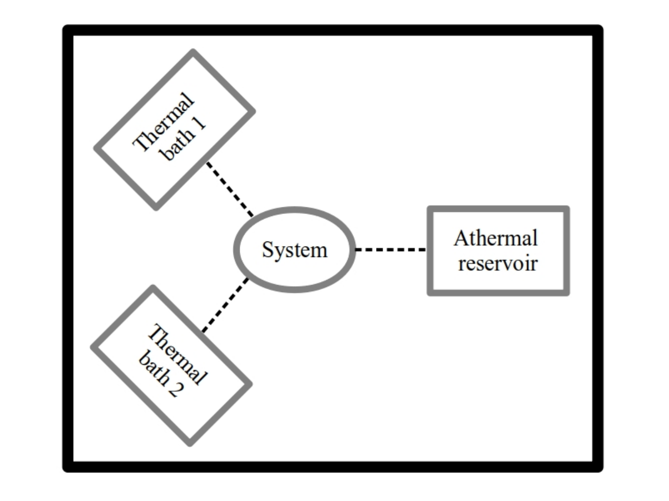
The Langevin force is a white Gaussian noise with cumulants
| (2) |
where is the effective temperature of thermal bath (the Boltzmann constant is assumed as ); and are respectively Kronecker and Dirac delta functions. We adopt the notation of double angle brackets for cumulants and single brackets for moments. The stochastic force is an external white noise with non-Gaussian properties van Kampen 2007. For simplicity, we consider that is unbiased and symmetric. The non-zero cumulants of the athermal noise are converging and given by
| (3) |
The odd cumulants are zero by construction, yielding an infinite number of even cumulants Marcinkiewicz 1939. The positive quantity presents dimension of impulse to the power of over one unit time (). In practice, we consider that is an unbiased Poisson noise with rate of events and impulses that follow a Gaussian distribution with zero mean and standard deviation Łuczka et al. 1997; Morgado and Queirós 2016:
| (4) |
Then, one finds
| (5) |
Observe that, although we are supposing an Poisson stochastic force, it is possible to obtain an external Gaussian noise by taking the limit , , with the product being constant van Kampen 2007; Łuczka et al. 1997; Morgado and Queirós 2016. This limiting case may be understood by writing in terms of as , with fixed. Thus, if is very large and , we have and only is non-zero when external kicks act in a very frequent way. Therefore, the type of external noise considered allows us to investigate the effects of athermal Gaussian and non-Gaussian fluctuations on a Brownian-type model with two distinct heat baths.
III Cumulant-generating function of position and velocity
The instantaneous position and velocity associated with the linear Langevin-like model (1) can be determined through the approach discussed in Tomé and de Oliveira 2015; Zwanzig 2001, even though we have a Poissonian noise. We write (1) in a matrix form
| (6) |
where
| (7) |
with and . Notice that (6) resembles a non-homogeneous system of linear differential equations with constant coefficients. Since is time-independent, the formal solution of (6) is
| (8) |
We calculate the exponential of matrix by using its eigenframe system:
| (9) |
where is the diagonal form of , is a matrix those columns are the right eigenvectors of , and is the inverse of . Suppose that is an eigenvalue of with associated right eigenvector . Then, after some calculation, one finds
| (10) |
where is the imaginary unit. Therefore, using (10) in (9), we obtain
| (11) |
where , and
| (12) |
Observe that is the complex conjugate of , and due to that are real-valued quantities.
The formal solutions (11) allow us to determine the time-dependent cumulants of and . Indeed, the variance of position is
| (13) |
where we have used the change of variable , and
| (14) |
A similar calculation lead to
| (15) |
Notice that is the average energy of the harmonic oscillator in steady-state regime:
| (16) |
| (17) |
For high-order cumulants of the type , with , and symmetric, one can find
| (18) |
where is assumed to be zero for odd. The integration over time variables and are performed without difficulties; the presence of delta functions simplifies the calculation. As a result, we obtain
| (19) |
where and are positive integers greater than two. Observe that in the limit , , with constant, we have , for , and only the second cumulants of and are different from zero, which means that the position and velocity are Gaussian stochastic variables when is very large with being fixed.
Since all the cumulants are determined in a closed form, we can make an attempt to find the cumulant-generating function related to the joint distribution of and :
| (20) |
where the conjugate variables are real. In our case—a linear stochastic system driven by independent noises—the generating function is a sum of two terms, , where
| (21) |
and
| (22) |
The function presents the effects of Gaussian thermal noises, and accounts for the contributions of non-thermal cumulants. The sums in (22) are allowed to run over all non-negative integer , provided that is different from zero for , with . Due to that, the sums may be rearranged appropriately, and remembering that , we have
| (23) |
The term within braces is simply a binomial expansion, which leads to
| (24) |
Now, by using the Gaussian identity
| (25) |
with and being real, we can set , which is in fact real, and obtain
| (26) |
where the average is taken over the Gaussian distribution defined in (4), with zero mean and variance . This distribution characterizes the statistics of impulse of external Poisson noise.
In addition, with the exact expressions of for given values of positive integers and , the long-time limit of cumulants of position and velocity can be evaluated, as least in principle. For the case of fourth-order cumulants, a direct calculation using (19) leads to
| (27) |
| (28) |
The stationary cumulant is zero. As a matter of fact, every cumulant of the type , with , tends to zero for steady-states:
| (29) |
where is a parameter independent of time. The result (29) is in agreement with Morgado 2015, which used a different theoretical approach. Indeed, it is possible to obtain an expression for the generating function (26) in the limit . Consider that in (10), which allows us to rewrite (12) as
| (30) |
Then, we set the change of variable , which is analogous to did in Fodor et al. 2018, but with a distinct prefactor and another relaxation time-scale. Notice that has dimension of second over mass (i.e., reciprocal viscous coefficient). After some algebraic manipulation, we have the stationary generating function
| (31) |
where
| (32) |
Notice that is negative. The exact expression of generating function (31) is valid for very long times , and represents the Poisson noise effects on the steady-state statistics of position and velocity of the trapped inertial particle.
Observe that in the limit , with constant, we have a Gaussian distribution for and that is only consistent with the equilibrium Boltzmann-Gibbs statistics, with well-defined canonical temperature, in the absence of external noise, and with equal bath temperatures. Indeed, we will see in the next section that the stationary state of the model presents non-zero energetic currents due to external noise effects and different temperatures of thermal sources. Therefore, in our context, the external noise contributes to driving the system out of equilibrium.
IV Stochastic heat and external work-like quantities
The main interest of this work is to investigate the heat exchanges and energy injected by external non-Gaussian stochastic force. For Langevin systems driven solely by Gaussian noises, it is possible to develop an analysis through the energetic concepts discussed in Sekimoto 1998; Sekimoto 2010; Gomez-Solano et al. 2010; Pal and Sabhapandit 2014. In such cases, heat is identified as the work performed by the sum of friction force and thermal noise Sekimoto 2010; the energetic contribution associated with the athermal environment may be given by the work done by external noise Gomez-Solano et al. 2010; Pal and Sabhapandit 2014. These work-like quantities are written as stochastic integrals of Stratonovich type Gardiner 2004; Sekimoto 2010. In this work, for the damped linear model given by (1), we assume that heat and external work can be interpreted analogously, despite the presence of non-Gaussian noise. We also consider calculus rules according to Stratonovich prescription.
Within the assumption mentioned above, we introduce the dimensionless heat associated with the thermal baths
| (33) |
and the dimensionless work-like quantity due to the non-Gaussian noise
| (34) |
where
| (35) |
It is also convenient to consider the additional dimensionless quantities
| (36) |
These non-dimensional variables simplify the analysis of expressions. It is straightforward to show that
| (37) |
The case with equal bath temperatures leads to and . For external Gaussian noise, which can be obtained by taking , , with , the quantity is the only relevant parameter associated with athermal medium. By analogy with the second cumulants of thermal noises, we may interpret as proportional to an dimensionless temperature-like quantity related to athermal reservoir. When the external noise is of Poisson kind, its stochastic properties depend on the parameters and .
According to our formulation, the energetic exchanges and are associated with different surroundings. Due to that, we understand it is reasonable to consider different quantities for each energetic contribution. Notice that and are correlated because the system—a Brownian particle trapped in a harmonic potential—is simultaneously coupled to different reservoirs.
Indeed, we may obtain information about the fluctuating behavior of and by evaluating their cumulants, as long as such calculation is possible. Then, by assuming the moments are feasible to determine, we follow a treatment analogous to the one discussed in Morgado and Duarte Queirós 2014; Morgado and Queirós 2016 in order to calculate the cumulants of energetic transfers. According to (33) and (34), and are given in terms of the instantaneous velocity and noises and . However, the velocity (11) is a superposition of independent stochastic forces. This allows us to write the moments of and through time integrals involving moments of uncorrelated noises. We expand the moments of noises into cumulants, and the integrals are evaluated for very long times. With the expressions for the moments, we determine the long-term cumulants of and .
IV.1 Fluctuations of energy exchanged with athermal source: Gaussian case
For the limit of very small intensities and large Poisson rate , with fixed, i.e, , the athermal noise approaches a Gaussian stochastic force. This case is investigated in Sabhapandit 2011 with a single thermal noise. Nonetheless, in this work, we are supposing the action of two distinct heat sources and an external Gaussian process. The cumulants of can be determined by calculating its moments. The general expression of moment of order of is given by
| (38) |
This equation is valid for being a Gaussian or Poissonian stochastic force. Then, we write the moments in terms of cumulants; the integrals are performed and the main contributions for very long are considered. As a result, for Gaussian, one can find
| (39) |
| (40) |
| (41) |
| (42) |
where is the average energy of the system shown in (14). Now, using the relations between moments and cumulants van Kampen 2007; Gardiner 2004 and the dimensionless quantities (36), it is possible to show that
| (43) |
| (44) |
Although the system is coupled to two thermal baths and one athermal reservoir, the cumulants (43)–(44) are written only in terms of the dimensionless quantity . Then, if we consider the particular case where there exists just a single heat reservoir, for example, by taking , the first four cumulants of are still of the form (43)–(44) by adopting the dimensionless parameters (36).
Observe that, according to (43)–(44), the long-time limit of the distribution function of is not Gaussian: high-order cumulants beyond the second are different from zero. Indeed, the athermal energy is proportional to the time integral of the power , which is a product of Gaussian variables when external noise is Gaussian, and that type of product usually is not Gaussian. Also, the autocorrelation function of is
| (45) |
with , where is the Heaviside step function and is shown in (12). The velocity-velocity autocorrelation function in steady-state regime is given by , which decays exponentially in time difference . As a result, it is possible to perceive that (45) is zero for , but it is diverges when because is not well-defined in the white noise limit (see (3)). In fact, the variance of is singular when the noise is white, which is also obtained in Morgado and Duarte Queirós 2014; Morgado and Queirós 2016 for the case of a harmonic oscillator driven by a single white noise. A sum of stochastic variables, each one with infinity variance, does not fulfill the conditions of the Central Limit Theorem Gardiner 2004. Thus, it is reasonable that does not follow Gaussian statistics.
As we said before, when there is a single thermal reservoir (e.g., as ), in addition to an athermal Gaussian noise, the expressions of cumulants are still the same as shown in (43)–(44), but with and , since we are working with non-dimensional quantities. In this case, our calculation of the first cumulants of are in agreement with results discussed in Sabhapandit 2011; Sabhapandit 2012 for a inertial Brownian particle trapped in an harmonic well and subjected to thermal and athermal Gaussian stochastic forces. On the other hand, when the effects of external are dominant (i.e., for ), the cumulant-generating function of , which is of the form , can be written as a series expansion
| (46) |
Then, by assuming this series converges, we may try to rearrange the first terms in order to see if some elementary functions can be identified. In fact, this is possible and gives
| (47) |
which is consistent with the analysis presented in Farago 2002.
IV.2 First cumulants of energy injected by Poisson noise
When the Poisson rate and variance of impulse distribution are finite, the system is under the influence of a non-Gaussian stochastic force. In this case, by considering that is very long, time-independent contributions can be disregarded in calculating the moments of . Consequently, we find
| (48) |
| (49) |
| (50) |
The cumulants are obtained through the expressions , and , which lead to
| (51) |
| (52) |
| (53) |
where the dimensionless quantities (36) are adopted. Observe that, for being Poissonian van Kampen 2007, the quantity is the average number of impulses in the interval . As a result, we may interpret as the mean dimensionless energy per impulse injected by the Poisson noise.
We also evaluate the averages of products of and :
| (54) |
For very long times (), we have
| (55) |
Then, in terms of non-dimensional quantities, the covariances can be written as
| (56) |
We see that the average injected energy (fisrt cumulant ), the standard deviation (square root of ) and the asymmetry (third cumulant ) of the distribution of depend on the dimensionless quantities and . These parameters are proportional to the Poisson rate and impulse variance , which are related to external noise cumulants (3)–(5). Then, the quantities are influenced by the cumulants of , i.e., the non-Gaussian fluctuations due to external noise contribute to the fluctuations of energy injection . This may be important for the energetic considerations of mesoscopic systems driven by external stochastic forces, since the nature of noise affects the statistics of energy exchanges with the reservoirs. For example, in the context of microsized engines investigated experimentally in Dinis et al. 2016; Roy et al. 2021. Notice that the covariances are always less than or equal to zero, as well as proportional to , where the coefficient of proportionality is , which is related to the friction coefficient that represents the coupling to thermal bath. It is straightforward to check that in the limit of very high rate and fixed, one can recover the cumulants (43)–(44) for the case of external Gaussian noise. On the other hand, in the limit of small temperatures ( large), and considering , the expressions for , , written in appropriate units, are in agreement with Morgado and Queirós 2016.
Although we focus on the long-time limit, the expression of second cumulant of is feasible to be shown for any value of :
| (57) |
where
| (58) |
The first term in (57) is proportional to , which leads to the main contribution when . There is also a term that decays exponentially with time and only contributes in a significant way in the transient regime. Notice that (57) does not depend explicitly on and . The equation for the instantaneous third cumulant is long and complicated to be written here, but it also depends only on and , with one term linear in and another that vanishes exponentially for . We show in Fig. 2 the time dependence of second and third cumulants of , where it is possible to identify the evolution to a long-term regime in which scale with . It is worth mentioning that the first cumulant of is given by (51) for any positive.
The presence of non-zero third cumulant (i.e. the skewness) is an indication of non-Gaussian behavior related to . In fact, the stochastic power is a product of Gaussian and non-Gaussian variables, and probably is non-Gaussian. In addition, for an external Poissonian , the autocorrelation function of is given by
| (59) |
where is the Heaviside step function. The first term in (59) is due to the non-Gaussian nature of athermal noise and tends to zero in the Gaussian limit of , which leads to the particular case (45). Clearly, the autocorrelation function as well as the variance are singular quantities as long as is white. This is in agreement with the results found in Morgado and Queirós 2016 for a single stochastic force of Poisson kind. Therefore, the time-integrated variable is not expected to be Gaussian. Observe that, according to results discussed in IV.1, the fluctuations of are also non-Gaussian when is a Gaussian noise. Nevertheless, it is important to emphasize that, for being a Poisson-type noise, its non-Gaussian aspects influence in a distinct way, as indicated by cumulants shown in (51)-(53).
IV.3 Averages and covariances of heat
Again, using the formal solutions of Langevin-like system (11) and the cumulants of noises (2)–(3), we obtain the averages heat
| (60) |
| (61) |
where is defined in (58). The time-dependent averages present terms linear in , which is the relevant contribution for very long times, terms that becomes exponentially small for , in addition to terms that do not depend on time. We show in Fig. 3 graphs of the averages of against for different values of dimensionless parameters. In the long-time limit (), the first cumulants of are given by
| (62) |
| (63) |
Roughly speaking, the averages present some similarities with the macroscopic thermal exchanges of energy between the system and heat baths. Indeed, let us consider the steady-state mean currents and such as and , with . These average energetic currents lead to a kind of first law form (conservation of energy): , which gives . Now, suppose that , with . Then, we have and , which means that heat is flowing through the system from reservoir to bath . Otherwise, if , but keeping , we find and , which show that heat is delivered to thermal baths. As a result, we have two scenarios: there exists average heat flowing through the system from hotter bath to colder one, or thermal environments absorb (on average) the energy injected by external noise.
For the particular case with a single thermal bath, for example, if and , there is a current of energy from athermal source to heat reservoir: , . Here, it is possible to perceive an interesting connection with the use of electric shaking as a heating mechanism in Roßnagel et al. 2016. In this case, energy in the form of heat, which originally comes from the external work done upon the system, is pumped into the thermal reservoir—exactly as another source of heat at higher temperature would have done. Indeed, for mesoscopic fluctuating engines, external noises can be used to design reservoir-like effects Dinis et al. 2016; Roy et al. 2021. Then, the role of Gaussian and non-Gaussian external driving can be a point of interest. Observe that, for Poissonian and also considering and zero, the average heat current dissipated in the thermal bath depends on the rate of kicks and the mean dimensionless injected energy , both accessible experimentally in principle. In addition, according to (56), and are negatively correlated, where the covariance decreases as and increase. Alternatively, by assuming the change of variable , we have and . As a result, the average currents and present the same form for Gaussian (, finite) and Poissonian noises, but the expressions of and depend on the noise considered. This show the influence of the nature of the external stochastic force on the fluctuations of energy transfers.
It is also important to consider the effects of external noise on the covariances of . The general expression of second moments of heat is
| (64) |
We determine each contribution of (64) in a similar way to did in IV.1 and IV.2. Then, after performing the cumulant expansion of moments of noises as well as the time integrals, we find
| (65) |
where
| (66) |
| (67) |
| (68) |
| (69) |
with given by (14). These expressions allow us to write the cumulants . As a result, we obtain the variances of and :
| (70) |
| (71) |
The covariance of and are given by
| (72) |
Observe that the second cumulants of and are elements of the covariance matrix associated with the joint distribution of and .
The variances of and are influenced by the properties of external noise, as well as the temperatures of thermal reservoirs and friction coefficients. The same is true for the second cumulant . Notice that the quantity can be interpreted as the diffusion coefficient associated with the stochastic flow of heat . Analogously, would be the diffusion coefficient related to . By neglecting the effects of external noise (i.e. ), one can obtain
| (73) |
which is in agreement with Fogedby and Imparato 2011 by using the non-dimensional variables (36). In the Gaussian limit of external noise (, constant), we have
| (74) |
| (75) |
where the term proportional to vanishes. Indeed, we see that the external noise acts increasing the standard deviation of the distribution of . In particular, when is a compound Poisson noise, the fluctuations of are affected by the rate of kicks and the statistics of noise intensities. Thus, Gaussian or non-Gaussian stochastic forces influence in different ways the fluctuating behavior of thermal energies exchanged with heat baths.
We see that the covariance can be positive or negative; the sign depends on the values taken by the parameters of the model, as shown in Fig. 4 (a). Since the cumulant may change its sign, it is possible that can be zero: we may have uncorrelated heat fluctuations. However, even in such cases, and are correlated, as long as is non-zero and the effects of external noise are not negligible.
In the absence of the athermal reservoir, which is equivalent to taking , the covariance of and is negative,
| (76) |
and if the temperatures are different, heat flows on average from one thermal source to the other,
| (77) |
This is reasonable because indicates how the fluctuations of are correlated with the ones of : one thermal bath delivers and the other absorbs heat. When the external noise is Gaussian, we have:
| (78) |
where , with fixed. The quantity is negative as thermal environments effects are more important ( small); but it is positive when the effects of athermal reservoir dominate ( large). Indeed, according to (62)–(63) with , the increasing of favors negative. Then, both thermal reservoirs tend to receive heat due to the athermal energy injection when is large.
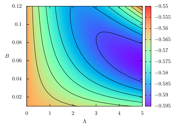
Also, observe that (78) is a convex quadratic function of , provided that the remaining parameters are fixed. Since is non-negative, one can show that (78) is zero when , and there exists a minimum in the graph of at , which is possible as long as . Then, the covariance may exhibit a non-monotonic behavior as a function of the parameter associated with the strength of the external Gaussian noise, see Fig. 4 (b). Nevertheless, it is important to bear in mind that the topography of the graph of can be more complicated because of the dependence on other parameters, i.e., and . Notice these features are for being an external Gaussian noise.
When is an athermal noise of Poisson kind, we perceive the emergence of a minimum in the graph of in the region of large and small, as shown in Fig. 5, which is consistent with the findings for the Gaussian limit of external noise. It is possible to interpret the sign of by assuming that and are fixed. Then, according to (72), if is constant, i.e. for a given mean injected energy per Poisson impulse, we have that is negative when is small and positive for large. Thus, a very low density number of kicks with finite mean energy does not modify the long-run tendency of heat to flow from hot to cold thermal baths. On the other hand, by supposing a given Poisson rate , we see that is negative if is small and positive when is large: the energetic effects of dominant athermal noise favor the absorption of heat by thermal baths.
We like to mention that our results are obtained by assuming and in (36) as independent quantities, and the Gaussian limit of external noise is obtained by taking , , constant. If we write and consider that and are now the new independent non-dimensional parameters related to non-Gaussian noise effects, we would find apparently distinct results. For example, in the equations of high-order cumulants of and shown in (52)–(53) and (70)–(72), we may rewrite , and the limit of small with fixed gives a quantity that is very large. We can deal with that by assuming also very small in order to find a term that approaches zero.
Independent of the kind of noise adopted in our model system, the study of work and heat correlations should be done with care because we also have to consider the temperatures of heat baths. Indeed, our analysis shows that, for a two-temperature Langevin system, the inclusion of external noise may promote non-trivial fluctuations of energetic quantities. On the other hand, for a given non-deterministic system, the coupling to a single or many thermal baths can lead to interesting and unusual power fluctuations.
V Conclusion
We investigated the non-equilibrium case of a damped Langevin-like model that represents an inertial Brownian particle in a harmonic potential and under the action of two thermal baths, at different temperatures, and an athermal reservoir, represented by an external Poisson noise. Since we have a linear stochastic model driven by independent noises, formal solutions are obtained without difficulties, which allow us to calculate all the time-dependent cumulants of position and velocity of the particle. With these cumulants, we also determined the cumulant-generating function of and , as a function of time, as well as its expression for steady-states, which is given by an integral form calculated exactly.
We studied the stochastic properties of the energetic exchanges between the Brownian particle and the thermal and athermal reservoirs for stationary states. In fact, we determined the long-term behavior of first cumulants of the injected energy due to the external noise and the heat related to thermal baths, which are defined by using appropriate dimensionless variables. The harmonically confined particle achieves an out-of-equilibrium steady-state with non-zero heat currents related to thermal baths and external power due to the athermal reservoir. For the injected athermal energy, which is a non-Gaussian variable, we shown that the standard deviation and the asymmetry (third cumulant) of the distribution of are influenced by the rate of Poisson kicks and the statistics of noise impulses, as well as the properties of thermal baths. Also, we evaluated the covariance of heat exchanges, which present different behaviors if the external noise is Poissonian or Gaussian. This covariance, represented by the second cumulant , can be positive, negative and even zero, in addition to have a non-monotonic behavior in terms of the parameters of the model. Thus, the specific structure of external noise plays a prominent role in the correlations and fluctuations of heat exchanges.
Acknowledgements.
This study was financed in part by the Coordenação de Aperfeiçoamento de Pessoal de Nível Superior - Brasil (CAPES) - Finance Code 001.References
- Callen (1960) H. B. Callen, Thermodynamics (John Wiley & Sons, Inc., 1960).
- Joule (1850) J. P. Joule, Phylosophical Transactions of the Royal Society of London 140, 61 (1850).
- Sekimoto (2010) K. Sekimoto, Stochastic Energetics (Springer Berlin Heidelberg, 2010).
- Sekimoto (1998) K. Sekimoto, Progress of Theoretical Physics Supplement 130, 17 (1998).
- Bustamante et al. (2005) C. Bustamante, J. Liphardt, and F. Ritort, Physics Today 58, 43 (2005), https://doi.org/10.1063/1.2012462 .
- Seifert (2012) U. Seifert, Reports on Progress in Physics 75, 126001 (2012).
- Holubec (2014) V. Holubec, Non-equilibrium Energy Transformation Processes (Springer International Publishing, 2014).
- Ciliberto (2017) S. Ciliberto, Phys. Rev. X 7, 021051 (2017).
- Speck et al. (2007) T. Speck, V. Blickle, C. Bechinger, and U. Seifert, EPL (Europhysics Letters) 79, 30002 (2007).
- Gomez-Solano et al. (2010) J. R. Gomez-Solano, L. Bellon, A. Petrosyan, and S. Ciliberto, EPL (Europhysics Letters) 89, 60003 (2010).
- Saha et al. (2009) A. Saha, S. Lahiri, and A. M. Jayannavar, Phys. Rev. E 80, 011117 (2009).
- Morgado and Soares-Pinto (2010) W. A. M. Morgado and D. O. Soares-Pinto, Phys. Rev. E 82, 021112 (2010).
- Blickle and Bechinger (2011) V. Blickle and C. Bechinger, Nature Phys. 8, 143 (2011).
- Fogedby and Imparato (2014) H. C. Fogedby and A. Imparato, J. Stat. Mech. 2014, P11011 (2014).
- Argun et al. (2017) A. Argun, J. Soni, L. Dabelow, S. Bo, G. Pesce, R. Eichhorn, and G. Volpe, Phys. Rev. E 96, 052106 (2017).
- Albay et al. (2021) J. A. C. Albay, Z.-Y. Zhou, C.-H. Chang, and Y. Jun, Sci. Rep. 11 (2021), 10.1038/s41598-021-83824-7.
- Holubec and Marathe (2020) V. Holubec and R. Marathe, Phys. Rev. E 102, 060101 (2020).
- Sabhapandit (2012) S. Sabhapandit, Phys. Rev. E 85, 021108 (2012).
- Fogedby and Imparato (2011) H. C. Fogedby and A. Imparato, Journal of Statistical Mechanics: Theory and Experiment 2011, P05015 (2011).
- Wang et al. (2002) G. M. Wang, E. M. Sevick, E. Mittag, D. J. Searles, and D. J. Evans, Phys. Rev. Lett. 89, 050601 (2002).
- Farago (2002) J. Farago, Journal of Statistical Physics 107, 781 (2002).
- Pal and Sabhapandit (2014) A. Pal and S. Sabhapandit, Phys. Rev. E 90, 052116 (2014).
- Gupta and Sabhapandit (2017) D. Gupta and S. Sabhapandit, Phys. Rev. E 96, 042130 (2017).
- Touchette and Cohen (2007) H. Touchette and E. G. D. Cohen, Phys. Rev. E 76, 020101 (2007).
- Baule and Cohen (2009) A. Baule and E. G. D. Cohen, Phys. Rev. E 80, 011110 (2009).
- Medeiros and Duarte Queirós (2015) J. R. Medeiros and S. M. Duarte Queirós, Phys. Rev. E 92, 062145 (2015).
- Duarte Queirós (2016) S. M. Duarte Queirós, Phys. Rev. E 94, 042114 (2016).
- Mestres et al. (2014) P. Mestres, I. A. Martinez, A. Ortiz-Ambriz, R. A. Rica, and E. Roldan, Phys. Rev. E 90, 032116 (2014).
- Dinis et al. (2016) L. Dinis, I. A. Martínez, É. Roldán, J. M. R. Parrondo, and R. A. Rica, Journal of Statistical Mechanics: Theory and Experiment 2016, 054003 (2016).
- Roßnagel et al. (2016) J. Roßnagel, S. T. Dawkins, K. N. Tolazzi, O. Abah, E. Lutz, F. Schmidt-Kaler, and K. Singer, Science 352, 325 (2016), arXiv:1510.03681 .
- Park et al. (2020) J. T. Park, G. Paneru, C. Kwon, S. Granick, and H. K. Pak, Soft Matter 16, 8122 (2020).
- Roy et al. (2021) N. Roy, N. Leroux, A. K. Sood, and R. Ganapathy, Nature Communications 12 (2021), 10.1038/s41467-021-25230-1.
- Kubo (1957) R. Kubo, Journal of the Physical Society of Japan 12, 570 (1957).
- Hansen and McDonald (2013) J.-P. Hansen and I. McDonald, Theory of Simple Liquids, 4th ed. (Academic Press, New York, 2013).
- de Groot and Mazur (2011) S. R. de Groot and P. Mazur, Non-Equilibrium Themodynamics (Dover, New York, 2011).
- Morgado et al. (2011) W. A. M. Morgado, S. M. D. Queirós, and D. O. Soares-Pinto, Journal of Statistical Mechanics: Theory and Experiment 2011, P06010 (2011).
- Morgado and Queirós (2016) W. A. M. Morgado and S. M. D. Queirós, Phys. Rev. E 93, 012121 (2016).
- Kanazawa (2017) K. Kanazawa, Statistical Mechanics for Athermal Fluctuations (Springer Thesis, 2017).
- Kanazawa et al. (2013) K. Kanazawa, T. Sagawa, and H. Hayakawa, Phys. Rev. E 87, 052124 (2013).
- Kanazawa et al. (2015) K. Kanazawa, T. G. Sano, T. Sagawa, and H. Hayakawa, Phys. Rev. Lett. 114, 090601 (2015).
- van Kampen (2007) N. G. van Kampen, Stochastic Processes in Physics and Chemistry, 3rd ed. (North-Holland, Amsterdam, 2007).
- Lee et al. (2013) J. S. Lee, C. Kwon, and H. Park, Phys. Rev. E 87, 020104 (2013).
- Marcinkiewicz (1939) J. Marcinkiewicz, Mathematische Zeitschrift 44, 612 (1939).
- Łuczka et al. (1997) J. Łuczka, T. Czernik, and P. Hänggi, Phys. Rev. E 56, 3968 (1997).
- Tomé and de Oliveira (2015) T. Tomé and M. J. de Oliveira, Stochastic Dynamics and Irreversibility, 1st ed. (Springer-Verlag, 2015).
- Zwanzig (2001) R. Zwanzig, Nonequilibrium Statistical Mechanics (Oxford Press, Oxford, New York, Heidelberg, 2001).
- Morgado (2015) W. Morgado, Physica A: Statistical Mechanics and its Applications 438, 493 (2015).
- Fodor et al. (2018) E. Fodor, H. Hayakawa, J. Tailleur, and F. van Wijland, Phys. Rev. E 98, 062610 (2018).
- Gardiner (2004) C. W. Gardiner, Handbook of Stochastic Methods for Physics, Chemistry, and the Natural Sciences, 3rd ed. (Springer International Publishing, 2004).
- Morgado and Duarte Queirós (2014) W. A. M. Morgado and S. M. Duarte Queirós, Phys. Rev. E 90, 022110 (2014).
- Sabhapandit (2011) S. Sabhapandit, EPL (Europhysics Letters) 96, 20005 (2011).