跳到论文正文
W Papers独立论文阅读器 arXiv:2104.01095 论文正文 计算阅读时间 · 0%
引用这篇论文根据当前论文元数据生成,正式投稿前建议核对。


License: arXiv.org perpetual non-exclusive license
arXiv:2104.01095v2 [math.AP] 25 Jun 2021

Quantitative dynamics of irreversible enzyme reaction-diffusion systemsThanks: We would like to thank Ján Eliaš for the discussion concerning the case of non-diffusive enzyme and complex molecules.
The third author has been partially supported by NAWI Graz.

Marcel Braukhoff Address: Marcel Braukhoff Mathematisches Institut der Heinrich Heine Universität Düsseldorf, Universitätsstraße 1, D-40225 Düsseldorf, Germany Email address: marcel.braukhoff@hhu.de , Amit Einav Address: Amit Einav School of Mathematical Sciences, Durham University, Upper Mountjoy Campus, Stockton Road DH1 3LE Durham, United Kingdom Email address: amit.einav@durham.ac.uk and Bao Quoc Tang Address: Bao Quoc Tang Institute of Mathematics and Scientific Computing, University of Graz, Heinrichstrasse 36, 8010 Graz, Austria Email address: quoc.tang@uni-graz.at, baotangquoc@gmail.com
Abstract.

In this work we investigate the convergence to equilibrium for mass action reaction-diffusion systems which model irreversible enzyme reactions. Using the standard entropy method in this situation is not feasible as the irreversibility of the system implies that the concentrations of the substrate and the complex decay to zero. The key idea we utilise in this work to circumvent this issue is to introduce a family of cut-off partial entropy functions which, when combined with the dissipation of a mass like term of the substrate and the complex, yield an explicit exponential convergence to equilibrium. This method is also applicable in the case where the enzyme and complex molecules do not diffuse, corresponding to chemically relevant situation where these molecules are large in size.

Key words: Enzyme Reactions; Reaction-Diffusion Systems; Irreversibility; Entropy Method; Degenerate Diffusion
MSC. 35B40, 35K57, 35Q92, 80A30, 92C45

1. Introduction

The focus of our work will be on the well known irreversible enzyme reaction system

(1.1) E+S​⇆kfkr​C→kcE+PE+S\underset{k_{f}}{\overset{k_{r}}{\leftrightarrows}}C\xrightarrow{k_{c}}E+P

where SS represents the substrate of the system, EE the enzymes, CC the intermediate complex (which we will refer to as the complex for simplicity) and PP the product.

1.1. The setting of the problem

Our study will concern itself with the inhomogeneous setting of (1.1) which manifests itself in the presence of diffusion of (some of) the system’s elements. By applying Fick’s law of diffusion and the law of mass action we find that the reaction-diffusion system that corresponds to (1.1) is given by

(1.2) {∂te⁡(x,t)−de​Δ​e​(x,t)=−kf​e​(x,t)​s​(x,t)+(kr+kc)​c​(x,t),x∈Ω,t>0,∂ts⁡(x,t)−ds​Δ​s​(x,t)=−kf​e​(x,t)​s​(x,t)+kr​c​(x,t),x∈Ω,t>0,∂tc⁡(x,t)−dc​Δ​c​(x,t)=kf​e​(x,t)​s​(x,t)−(kr+kc)​c​(x,t),x∈Ω,t>0,∂tp⁡(x,t)−dp​Δ​p​(x,t)=kc​c​(x,t),x∈Ω,t>0,de​∂νe⁡(x,t)=ds​∂νs⁡(x,t)=dc​∂νc⁡(x,t)=dp​∂νp⁡(x,t)=0,x∈∂Ω,t>0,e(x,0)=e0(x),s(x,0)=s0(x),c(x,0)=c0(x),p(x,0)=p0(x),x∈Ω,\begin{cases}\partial_{t}e(x,t)-d_{e}\Delta e(x,t)=-k_{f}e(x,t)s(x,t)+(k_{r}+k_{c})c(x,t),&x\in\Omega,t>0,\\ \partial_{t}s(x,t)-d_{s}\Delta s(x,t)=-k_{f}e(x,t)s(x,t)+k_{r}c(x,t),&x\in\Omega,t>0,\\ \partial_{t}c(x,t)-d_{c}\Delta c(x,t)=k_{f}e(x,t)s(x,t)-(k_{r}+k_{c})c(x,t),&x\in\Omega,t>0,\\ \partial_{t}p(x,t)-d_{p}\Delta p(x,t)=k_{c}c(x,t),&x\in\Omega,t>0,\\ {d_{e}\partial_{\nu}e(x,t)=d_{s}\partial_{\nu}s(x,t)=d_{c}\partial_{\nu}c(x,t)=d_{p}\partial_{\nu}p(x,t)=0},&x\in\partial\Omega,t>0,\\ e(x,0)=e_{0}(x),\;s(x,0)=s_{0}(x),\;c(x,0)=c_{0}(x),\;p(x,0)=p_{0}(x),&x\in\Omega,\end{cases}

where e⁡(x,t),s⁡(x,t),c⁡(x,t),p⁡(x,t)e(x,t),s(x,t),c(x,t),p(x,t) are the concentrations of EE, SS, CC and PP, respectively, at x∈Ωx\in\Omega and t>0t>0. The homogeneous Neumann boundary condition indicates that the system is closed, and in order that the equations would make chemical sense we also require that the initial concentrations e0​(x),s0​(x)e_{0}(x),s_{0}(x), c0​(x)c_{0}(x) and p0​(x)p_{0}(x) are non-negative functions11 1 As the Neumann condition is connected to the diffusion of the concentration, we have elected to write it as de​∂νe⁡(x,t)=ds​∂νs⁡(x,t)=dc​∂νc⁡(x,t)=dp​∂νp⁡(x,t)=0d_{e}\partial_{\nu}e(x,t)=d_{s}\partial_{\nu}s(x,t)=d_{c}\partial_{\nu}c(x,t)=d_{p}\partial_{\nu}p(x,t)=0 to indicate that we do not require it when the diffusion coefficient is zero..

Looking at the system (1.2), one notices immediately that the equation that governs the concentration of PP, p⁡(x,t)p(x,t), is decoupled from the rest of the system and is completely solvable once c⁡(x,t)c(x,t) has been found. Therefore, our main focus in the majority of this work will be on the dynamics of the sub-system of (1.2) which includes ee, ss and cc alone.

Much like many other reaction-diffusion systems in a bounded domain, one expects that the combination of the chemical reactions and the diffusion will result in a state of equilibrium that is composed of constant concentrations. Using the (formal) conservation laws

(1.3) ∫Ω(e⁡(x,t)+c⁡(x,t))​𝑑x=M0:=∫Ω(e0​(x)+c0​(x))​𝑑x,∀t≥0,\int_{\Omega}(e(x,t)+c(x,t))dx=M_{0}:=\int_{\Omega}(e_{0}(x)+c_{0}(x))dx,\quad\forall t\geq 0,
(1.4) ∫Ω(s⁡(x,t)+c⁡(x,t)+p⁡(x,t))​𝑑x=M1:=∫Ω(s0​(x)+c0​(x)+p0​(x))​𝑑x,∀t≥0,\int_{\Omega}(s(x,t)+c(x,t)+p(x,t))dx=M_{1}:=\int_{\Omega}(s_{0}(x)+c_{0}(x)+p_{0}(x))dx,\quad\forall t\geq 0,

and under the assumption that |Ω|=1\left\lvert\Omega\right\rvert=1 for simplicity (which can always be achieved by a simple rescaling of the spatial variable) we find that if all elements in the system diffuse, i.e. if de,ds,dcd_{e},d_{s},d_{c} and dpd_{p} are strictly positive, then the equations that determine the constant equilibrium concentrations e∞,c∞,s∞e_{\infty},c_{\infty},s_{\infty} and p∞p_{\infty} are

{−kf​e∞​s∞+(kr+kc)​c∞=0,−kf​e∞​s∞+kc​c∞=0,kc​c∞=0e∞+c∞=M0,s∞+c∞+p∞=M1,\begin{cases}-k_{f}e_{\infty}s_{\infty}+(k_{r}+k_{c})c_{\infty}=0,\\ -k_{f}e_{\infty}s_{\infty}+k_{c}c_{\infty}=0,\\ k_{c}c_{\infty}=0\\ e_{\infty}+c_{\infty}=M_{0},\\ s_{\infty}+c_{\infty}+p_{\infty}=M_{1},\end{cases}

from which we find that

e∞=M0,c∞=0,s∞=0,p∞=M1.e_{\infty}=M_{0},\quad c_{\infty}=0,\quad s_{\infty}=0,\quad p_{\infty}=M_{1}.

This equilibrium carries within it the chemical intuition of the process, as was expected: As time increases, the substrates get completely converted into product, the complex is used up, and the enzymes “gobble up” whatever left overs remain in the system.

The above, however, is not the true equilibrium when essential parts of the system do not diffuse. In this case, we can’t a-priori guarantee that an equilibrium state for these non-diffusing concentration, if one exists, will be a constant function. This situation is chemically feasible, for instance when the molecules of the complex and the enzymes are large enough to deter diffusion. In terms of our system (1.2) this situation corresponds to the case where de=dc=0d_{e}=d_{c}=0 and dsd_{s} and dpd_{p} are strictly positive. The lack of diffusion in the complex cc is not very problematic, yet the lack of diffusion in the enzymes ee complicates matter further. However, in this situation one can find another (formal) conservation law of the form22 2 In this case we have that ∂t(e⁡(x,t)+c⁡(x,t))=0\partial_{t}\left(e(x,t)+c(x,t)\right)=0.

(1.5) e⁡(x,t)+c⁡(x,t)=e0​(x)+c0​(x),e(x,t)+c(x,t)=e_{0}(x)+c_{0}(x),

which assists in balancing the system. With this in mind, we see that if an equilibrium of the form e∞​(x)e_{\infty}(x), c∞​(x)c_{\infty}(x) and s∞s_{\infty} exists 33 3 The equilibrium for ee and cc could be a function of xx, but s∞s_{\infty} is still assumed to be constant due to the diffusion in ss., then it must satisfy

{−kf​e∞​(x)​s∞+(kr+kc)​c∞​(x)=0,−kf​e∞​(x)​s∞+kc​c∞​(x)=0,e∞​(x)+c∞​(x)=e0​(x)+c0​(x),\begin{cases}-k_{f}e_{\infty}(x)s_{\infty}+(k_{r}+k_{c})c_{\infty}(x)=0,\\ -k_{f}e_{\infty}(x)s_{\infty}+k_{c}c_{\infty}(x)=0,\\ e_{\infty}(x)+c_{\infty}(x)=e_{0}(x)+c_{0}(x),\\ \end{cases}

from which we find that s∞=c∞​(x)=0s_{\infty}=c_{\infty}(x)=0 and e∞​(x)=e0​(x)+c0​(x)e_{\infty}(x)=e_{0}(x)+c_{0}(x). The fact that c∞​(x)=0c_{\infty}(x)=0 would lead us to expect that p⁡(x,t)p(x,t) also converges to a constant p∞p_{\infty} and due to (1.4) we conclude that the suspected equilibrium in this case is given by

(1.6) e∞​(x)=e0​(x)+c0​(x)s∞=c∞​(x)=0,p∞=M1.e_{\infty}(x)=e_{0}(x)+c_{0}(x)\,\quad s_{\infty}=c_{\infty}(x)=0,\quad p_{\infty}=M_{1}.

The main goal of our work is to explicitly and quantitatively explore the rate of convergence to equilibrium of the solutions to (1.2) in these two cases in the strongest form possible - the L∞L^{\infty} norm.

1.2. Known results

The study of the trend to equilibrium for (bio-)chemical reaction-diffusion systems has witnessed significant progress in the last decades. The first results in this direction can be attributed to [Grö83, Grö92, GGH96] where the large time behaviour of two dimensional such systems was studied qualitatively. Quantitative results, i.e. explicit convergence rates and constants, have been provided in [DF06, DF08] for special systems, and have been extended later in [DFT17, MHM15] to more complicated ones. The most general equilibration results, which are currently feasible, are those found in [Mie16, FT18]. Despite these developments and advances, the quantitative large time behaviour of the enzyme reaction-diffusion system (1.2) was, to our knowledge, left completely untouched. The main reason, in our opinion, for this omission lies with the irreversible nature of (1.1), and its impact the entropy method which is commonly used to investigate quantitative long time behaviour. We shall address this point shortly, as our work will show how one can “modify” this method to attain our claimed results.

1.3. Main results

As was indicated in the end of §1.1, our work is devoted to the investigation of two cases for the system 1.2. Our main results can be expressed by the following theorems:

Theorem 1.1.

Let Ω⊂ℝn\Omega\subset\mathbb{R}^{n} be a bounded, open domain with C2+ζC^{2+\zeta}, ζ>0\zeta>0, boundary, ∂Ω\partial\Omega. Assume that de,ds,dcd_{e},d_{s},d_{c} and dpd_{p} are strictly positive constants and that the initial data e0​(x),s0​(x),c0​(x)e_{0}(x),s_{0}(x),c_{0}(x) and p0​(x)p_{0}(x) are all bounded non-negative functions. Then there exists a unique non-negative bounded classical solution to (1.2). Moreover, there exists an explicit γ>0\gamma>0 such that for any η>0\eta>0 there exists an explicit constant 𝒞η\mathcal{C}_{\eta}, depending only on geometric properties and the initial data which blows up as η\eta goes to zero, such that

(1.7) ‖c⁡(t)‖L∞​(Ω)+‖s⁡(t)‖L∞​(Ω)≤𝒞η​e−2​γ​tn⁡(1+η),‖e⁡(t)−e∞‖L∞​(Ω)≤𝒞η​e−γ​tn⁡(1+η).\begin{gathered}\left\lVert c(t)\right\rVert_{L^{\infty}(\Omega)}+\left\lVert s(t)\right\rVert_{L^{\infty}(\Omega)}\leq\mathcal{C}_{\eta}e^{-\frac{2\gamma t}{n\left(1+\eta\right)}},\\ \left\lVert e(t)-e_{\infty}\right\rVert_{L^{\infty}(\Omega)}\leq\mathcal{C}_{\eta}e^{-\frac{\gamma t}{n\left(1+\eta\right)}}.\end{gathered}

In addition for any ε>0\varepsilon>0 and η>0\eta>0 with n⁡(1+η)≥4n\left(1+\eta\right)\geq 4 there exists an explicit constant 𝒞η,ε\mathcal{C}_{\eta,\varepsilon}, depending only on geometric properties and the initial data which blows up as η\eta or ε\varepsilon go to zero, such that

(1.8) ‖p⁡(t)−p∞‖L∞​(Ω)≤𝒞η,ε​(1+t4n⁡(1+η)​δ2​dpCP​(1−ε),γ)​e−min⁡(4​dpn​CP​(1+η)​(1−ε),2​γn⁡(1+η))​t\begin{gathered}\left\lVert p(t)-p_{\infty}\right\rVert_{L^{\infty}(\Omega)}\leq\mathcal{C}_{\eta,\varepsilon}\left(1+t^{\frac{4}{n\left(1+\eta\right)}\delta_{\mathchoice{\raisebox{-3.81477pt}{\resizebox{7465250}{655360}{\hbox{\raisebox{1.43054pt}{$\displaystyle\frac{2d_{p}}{C_{P}}\left(1-\varepsilon\right),\gamma$}}}}}{\raisebox{-3.33333pt}{\resizebox{6175146}{655360}{\hbox{\raisebox{1.25pt}{$\textstyle\frac{2d_{p}}{C_{P}}\left(1-\varepsilon\right),\gamma$}}}}}{\raisebox{-3.33333pt}{\resizebox{4995466}{655360}{\hbox{\raisebox{0.875pt}{$\scriptstyle\frac{2d_{p}}{C_{P}}\left(1-\varepsilon\right),\gamma$}}}}}{\raisebox{-4.59253pt}{\resizebox{5989482}{655360}{\hbox{\raisebox{0.8611pt}{$\scriptscriptstyle\frac{2d_{p}}{C_{P}}\left(1-\varepsilon\right),\gamma$}}}}}\mathstrut}}\right)e^{-\min\left(\frac{4d_{p}}{nC_{P}\left(1+\eta\right)}\left(1-\varepsilon\right),\frac{2\gamma}{n\left(1+\eta\right)}\right)t}\end{gathered}

where

δx,y={1x=y0x≠y\delta_{x,y}=\begin{cases}1&x=y\\ 0&x\not=y\end{cases}

and CPC_{P} is the Poincaré constant associated to the domain Ω\Omega.

Theorem 1.2.

Let Ω⊂ℝn\Omega\subset\mathbb{R}^{n} be a bounded, open domain with C2+ζ,ζ>0C^{2+\zeta},\zeta>0 boundary, ∂Ω\partial\Omega. Assume that dsd_{s} and dpd_{p} are strictly positive constants while de=dc=0d_{e}=d_{c}=0. Assume in addition that the initial data e0​(x)e_{0}(x), s0​(x)s_{0}(x), c0​(x)c_{0}(x) and p0​(x)p_{0}(x) are all bounded non-negative functions and that there exists some β>0\beta>0 such that

(1.9) e0​(x)+c0​(x)≥βa.e. ​x∈Ω.e_{0}(x)+c_{0}(x)\geq\beta\quad\text{a.e. }x\in\Omega.

Then there exists a unique non-negative bounded strong solution to (1.2). Moreover, there exists an explicit constant γ>0\gamma>0 such that for any η>0\eta>0 there exists an explicit constant 𝒞η\mathcal{C}_{\eta}, depending only on geometric properties and the initial data which blows up as η\eta goes to zero, such that

‖s⁡(t)‖L∞​(Ω)≤𝒞η​e−2​γn⁡(1+η)​t,‖e⁡(x,t)−e∞​(x)‖L∞​(Ω)+‖c⁡(t)‖L∞​(Ω)≤𝒞η​(1+tδkr+kc,2​γn⁡(1+η))​e−min⁡(kr+kc,2​γn⁡(1+η))​t.\begin{gathered}\|s(t)\|_{L^{\infty}(\Omega)}\leq\mathcal{C}_{\eta}e^{-\frac{2\gamma}{n\left(1+\eta\right)}t},\\ \|e(x,t)-e_{\infty}(x)\|_{L^{\infty}(\Omega)}+\|c(t)\|_{L^{\infty}(\Omega)}\leq\mathcal{C}_{\eta}\left(1+t^{\delta_{\mathchoice{\raisebox{-3.33333pt}{\resizebox{9299645}{655360}{\hbox{\raisebox{1.25pt}{$\displaystyle k_{r}+k_{c},\frac{2\gamma}{n\left(1+\eta\right)}\mathstrut$}}}}}{\raisebox{-2.79997pt}{\resizebox{6666049}{655360}{\hbox{\raisebox{0.97221pt}{$\textstyle k_{r}+k_{c},\frac{2\gamma}{n\left(1+\eta\right)}\mathstrut$}}}}}{\raisebox{-2.79996pt}{\resizebox{6174408}{655360}{\hbox{\raisebox{0.68054pt}{$\scriptstyle k_{r}+k_{c},\frac{2\gamma}{n\left(1+\eta\right)}\mathstrut$}}}}}{\raisebox{-3.33333pt}{\resizebox{7248933}{655360}{\hbox{\raisebox{0.625pt}{$\scriptscriptstyle k_{r}+k_{c},\frac{2\gamma}{n\left(1+\eta\right)}\mathstrut$}}}}}}}\right)e^{-\min\left(k_{r}+k_{c},\frac{2\gamma}{n\left(1+\eta\right)}\right)t}.\end{gathered}

In addition for any ε>0\varepsilon>0 and η>0\eta>0 with n⁡(1+η)≥4n\left(1+\eta\right)\geq 4 there exists an explicit constant 𝒞η,ε\mathcal{C}_{\eta,\varepsilon}, depending only on geometric properties and the initial data which blows up as η\eta or ε\varepsilon go to zero, such that

‖p⁡(t)−p∞‖L∞​(Ω)≤𝒞η,ε​(1+t4n⁡(1+η)​δ2​dpCP​(1−ε),γ)​e−min⁡(4​dpn​CP​(1+η)​(1−ε),2​γn⁡(1+η))​t\begin{gathered}\left\lVert p(t)-p_{\infty}\right\rVert_{L^{\infty}(\Omega)}\leq\mathcal{C}_{\eta,\varepsilon}\left(1+t^{\frac{4}{n\left(1+\eta\right)}\delta_{\mathchoice{\raisebox{-3.81477pt}{\resizebox{7465250}{655360}{\hbox{\raisebox{1.43054pt}{$\displaystyle\frac{2d_{p}}{C_{P}}\left(1-\varepsilon\right),\gamma$}}}}}{\raisebox{-3.33333pt}{\resizebox{6175146}{655360}{\hbox{\raisebox{1.25pt}{$\textstyle\frac{2d_{p}}{C_{P}}\left(1-\varepsilon\right),\gamma$}}}}}{\raisebox{-3.33333pt}{\resizebox{4995466}{655360}{\hbox{\raisebox{0.875pt}{$\scriptstyle\frac{2d_{p}}{C_{P}}\left(1-\varepsilon\right),\gamma$}}}}}{\raisebox{-4.59253pt}{\resizebox{5989482}{655360}{\hbox{\raisebox{0.8611pt}{$\scriptscriptstyle\frac{2d_{p}}{C_{P}}\left(1-\varepsilon\right),\gamma$}}}}}\mathstrut}}\right)e^{-\min\left(\frac{4d_{p}}{nC_{P}\left(1+\eta\right)}\left(1-\varepsilon\right),\frac{2\gamma}{n\left(1+\eta\right)}\right)t}\end{gathered}
Remark 1.3.

Our notion of strong solutions to (1.2) is as follows: For any p∈[1,∞)p\in[1,\infty), any component of the solution belongs to C⁡([0,∞),Lp​(Ω))C([0,\infty);L^{p}(\Omega)) and is absolutely continuous on (0,∞)(0,\infty) with respect to Lp​(Ω)L^{p}(\Omega). Moreover, the time derivatives, and the spatial derivatives up to second order of any concentration, which is diffusing, are in Lp​((τ,T),Lp​(Ω))L^{p}\left((\tau,T);L^{p}\left(\Omega\right)\right) for any T>τ>0T>\tau>0, and the equations and boundary conditions are satisfied a.e. in Ω×(0,T)\Omega\times(0,T) and a.e. in ∂Ω×(0,T)\partial\Omega\times(0,T) respectively, for any T>0T>0.

Remark 1.4.

During our proofs we will be able to provide an explicit form to γ\gamma in each of the theorems. We will show that one can choose

(1.10) γ=min\displaystyle\gamma=\min ((de​CLSI−6​((kc+kr)M0+kf)​max⁡(εc,εs))(1+(log⁡(1+M1εs)+k⁡(2​kr+kc)2​kr)​16​(εs+M1)(1−log⁡(2))​M0),\displaystyle\left(\frac{\left(d_{e}C_{\mathrm{LSI}}-6\left(\frac{\left(k_{c}+k_{r}\right)}{M_{0}}+k_{f}\right)\max\left(\varepsilon_{c},\varepsilon_{s}\right)\right)}{\left(1+\left(\log\left(1+\frac{M_{1}}{\varepsilon_{s}}\right)+\frac{k\left(2k_{r}+k_{c}\right)}{2k_{r}}\right)\frac{16\left(\varepsilon_{s}+M_{1}\right)}{\left(1-\log(2)\right)M_{0}}\right)},\right.
k​kc2−kc−kr−2​kf​εs(1+k+log⁡(1+M0εc)+(log⁡(1+M1εs)+k⁡(2​kr+kc)2​kr)​(2​krkf​M0+16​(εs+M1)(1−log⁡(2))​M0)),\displaystyle\frac{\frac{kk_{c}}{2}-k_{c}-k_{r}-2k_{f}\varepsilon_{s}}{\left(1+k+\log\left(1+\frac{M_{0}}{\varepsilon_{c}}\right)+\left(\log\left(1+\frac{M_{1}}{\varepsilon_{s}}\right)+\frac{k\left(2k_{r}+k_{c}\right)}{2k_{r}}\right)\left(\frac{2k_{r}}{k_{f}M_{0}}+\frac{16\left(\varepsilon_{s}+M_{1}\right)}{\left(1-\log(2)\right)M_{0}}\right)\right)},
OPENdc​ds​CLSIds+dc​(1+(log⁡(1+M1εs)+k⁡(2​kr+kc)2​kr)))\displaystyle\left.\frac{d_{c}d_{s}C_{\mathrm{LSI}}}{d_{s}+d_{c}\left(1+\left(\log\left(1+\frac{M_{1}}{\varepsilon_{s}}\right)+\frac{k\left(2k_{r}+k_{c}\right)}{2k_{r}}\right)\right)}\right)

with

(1.11) εc=CLSI​M012​(kc+kr+M0​kf)​max⁡(1,krM0​kf),εs=krM0​kfεc,k=4​(kc+kr+kf​εs)kc.\begin{gathered}\varepsilon_{c}=\frac{C_{\mathrm{LSI}}M_{0}}{12\left(k_{c}+k_{r}+M_{0}k_{f}\right)\max\left(1,\frac{k_{r}}{M_{0}k_{f}}\right)},\quad\varepsilon_{s}=\frac{k_{r}}{M_{0}k_{f}}\varepsilon_{c},\quad k=\frac{4\left(k_{c}+k_{r}+k_{f}\varepsilon_{s}\right)}{k_{c}}.\end{gathered}

for Theorem 1.1, where CLSIC_{\mathrm{LSI}} is the log-Sobolev constant that is associated to the domain Ω\Omega, and

(1.12) γ=\displaystyle\gamma= min⁡(k​kc2−kf​εs(1+k+log⁡(1+krkf​εs)+(log⁡(1+M1εs)+k⁡(2​kr+kc)2​kr)​(2​krkf​β+16​(εs+M1)(1−log⁡(2))​β))CLOSE\displaystyle\min\left(\frac{\frac{kk_{c}}{2}-k_{f}\varepsilon_{s}}{\left(1+k+\log\left(1+\frac{k_{r}}{k_{f}\varepsilon_{s}}\right)+\left(\log\left(1+\frac{M_{1}}{\varepsilon_{s}}\right)+\frac{k\left(2k_{r}+k_{c}\right)}{2k_{r}}\right)\left(\frac{2k_{r}}{k_{f}\beta}+\frac{16\left(\varepsilon_{s}+M_{1}\right)}{\left(1-\log(2)\right)\beta}\right)\right)}\right.
OPENds​CLSI1+(log⁡(1+M1εs)+k⁡(2​kr+kc)2​kr)),\displaystyle\left.\frac{d_{s}C_{\mathrm{LSI}}}{1+\left(\log\left(1+\frac{M_{1}}{\varepsilon_{s}}\right)+\frac{k\left(2k_{r}+k_{c}\right)}{2k_{r}}\right)}\right),

with

(1.13) εs∈(0,∞),k=4​kf​εskc.\begin{gathered}\varepsilon_{s}\in\left(0,\infty\right),\quad k=\frac{4k_{f}\varepsilon_{s}}{k_{c}}.\end{gathered}

These choices choices are clearly far from optimal, though explicit. Optimal convergence rate is a subtle issue and remains open in most chemical reaction-diffusion systems. Some discussion about this issue in the case where all diffusion coefficients are strictly positive will be given in §4.3.

Remark 1.5.

In our analysis, the lower bound condition (1.9) is essential to be able to obtain the explicit exponential convergence to equilibrium. This condition is easily satisfied when we require that the initial enzyme concentration e0e_{0} is present everywhere in Ω\Omega. In the case where (1.9) does not hold numerical solutions suggest that convergence to equilibrium can still be expected, as is indicated in Fig. 1 in §4.4. A rigorous proof, however, remains an open problem.

A common method one employs to investigate the quantitative long time behaviour of chemical reaction-diffusion systems (and many other physically, chemically and biologically relevant equations) is the so-called entropy method: By considering the connection between a natural Lypunov functional of the system, the entropy, and its dissipation, usually via a functional inequality, one recovers an explicit rate of convergence to equilibrium. This convergence rate can be boosted up to stronger norms in many situations, at least as long as the system has some smoothing effects.

This method has been extremely successful in dealing with reaction-diffusion systems which model reversible reactions, see e.g. [DF06, MHM15, DFT17, FT18] and references therein. A fundamental property of these systems which help facilitate the entropy method is the existence of a strictly positive equilibrium, which allows the consideration of natural entropies such as the Boltzmann entropy (to be defined shortly). This property, however, is not necessarily true in most open or irreversible reaction systems, precluding the consideration of the aforementioned entropies and, in our opinion, resulting in a relatively sparse study of the quantitative large time behaviour of such systems. The current work serves, to our knowledge, as the first study in this direction for the well known enzyme reaction (1.1), and we believe that the method introduced herein will be applicable to many other open and irreversible systems,

Let us delve deeper into the entropies one encounters in the study of chemical reaction-diffusion systems, the issues of a zero equilibrium and how we propose to overcome it in this work.

A natural entropy to consider in many chemical reaction-diffusion systems is generated by the Boltzmann entropy function

(1.14) 𝔥⁡(x)=x​log⁡x−x+1,x≥0.\mathfrak{h}(x)=x\log x-x+1,\qquad x\geq 0.

In particular, one uses this entropy function to define a relative entropy functional that measures the “entropic distance” between a solution to an equation, f⁡(x)f(x), and its equilibrium f∞f_{\infty}:

(1.15) ℰ⁡(f|f∞)=∫Ωh⁡(f⁡(x)|f∞)​𝑑x\mathcal{E}(f|f_{\infty})=\int_{\Omega}h\left(f(x)|f_{\infty}\right)dx

where

(1.16) h⁡(x|y)=x​log⁡(xy)−x+y=y​𝔥​(xy),x,y>0.h\left(x|y\right)=x\log\left(\frac{x}{y}\right)-x+y=y\mathfrak{h}\left(\frac{x}{y}\right),\quad\quad x,y>0.

Both ℰ\mathcal{E} and hh are naturally not well defined when f∞=0f_{\infty}=0 which is exactly the equilibrium we have (or suspect) for our substrate and complex concentrations ss and cc. Similar issues occur when the equilibrium is spatially inhomogeneous, i.e. f∞=f∞​(x)f_{\infty}=f_{\infty}(x), with

|{x∈Ω|f∞​(x)=0}|>0.\left\lvert\left\{x\in\Omega\;|\;f_{\infty}(x)=0\right\}\right\rvert>0.

This situation can indeed occur, as was shown in [JR11] where one finds that f∞f_{\infty} can be a sum of Dirac masses.

The first key idea and strategy that will guide us in showing our main results is to modify our Boltzmann entropy by defining a new relative entropy function that is “cut” when the concentration becomes “small enough”:

(1.17) hε​(x|ε)={x​log⁡(xε)−x+εx≥ε,0x<ε.h_{\varepsilon}\left(x|\varepsilon\right)=\begin{cases}x\log\left(\frac{x}{\varepsilon}\right)-x+\varepsilon&x\geq\varepsilon,\\ 0&x<\varepsilon.\end{cases}

With this “cut-off” entropy, we will consider a partial entropy functional

ℋεc,εs​(e,s,c)=∫Ωh⁡(e⁡(x)|e∞)​𝑑x+∫Ωhεc​(c⁡(x)|εc)​𝑑x+∫Ωhεs​(s⁡(x)|εs)​𝑑x,\mathscr{H}_{\varepsilon_{c},\varepsilon_{s}}(e,s,c)=\int_{\Omega}h(e(x)|e_{\infty})dx+\int_{\Omega}h_{\varepsilon_{c}}(c(x)|\varepsilon_{c})dx+\int_{\Omega}h_{\varepsilon_{s}}(s(x)|\varepsilon_{s})dx,

where εc,εs\varepsilon_{c},\varepsilon_{s} are to be chosen in a meaningful way. It is not clear if ℋεc,εs\mathscr{H}_{\varepsilon_{c},\varepsilon_{s}} is decreasing along the evolution of the system. Moreover, as we expect cc and ss to converge to zero, we expect ℋεc,εs​(e,s,c)\mathscr{H}_{\varepsilon_{c},\varepsilon_{s}}(e,s,c) to eventually become dependent only on ee and e∞e_{\infty} for any fixed εc\varepsilon_{c} and εs\varepsilon_{s} - the smallness of ℋεc,εs​(e,s,c)\mathscr{H}_{\varepsilon_{c},\varepsilon_{s}}(e,s,c) can only give us information on the convergence of ee to e∞e_{\infty}.

This is the point where we introduce our second key idea: Combine this partial entropy functional with a sum of masses from the substrate and complex which decreases and, together with the partial entropy, will drive these concentration to zero44 4 One can think of this as a hypocoercivity idea.. This sum of masses will be of the form

ℳ⁡(s,c)=∫Ω(c⁡(x)+η​s​(x))​𝑑x\mathscr{M}(s,c)=\int_{\Omega}(c(x)+\eta s(x))dx

with a suitable choice of η>0\eta>0. The drive of the concentration towards zero by ℳ⁡(s,c)\mathscr{M}(s,c) is expressed by the fact that we will find an explicit mass density, 𝒹ℳ​(x)\mathcal{d}_{\mathscr{M}}(x), such that

(1.18) dd​tℳ(s,c)=−∫Ω𝒹ℳ(x)dx≤0.\frac{d}{dt}\mathscr{M}(s,c)=-\int_{\Omega}\mathcal{d}_{\mathscr{M}}(x)dx\leq 0.

With ℋεc,εs​(e,s,c)\mathscr{H}_{\varepsilon_{c},\varepsilon_{s}}(e,s,c) and ℳ⁡(s,c)\mathscr{M}(s,c) at hand we will define our total entropy functional to be

ℰεc,εs,k​(e,s,c)=ℋεc,εs​(e,s,c)+k​ℳ​(s,c)\mathcal{E}_{\varepsilon_{c},\varepsilon_{s},k}(e,s,c)=\mathscr{H}_{\varepsilon_{c},\varepsilon_{s}}(e,s,c)+k\mathscr{M}(s,c)

for an appropriately chosen constant k>0k>0.

Showing the exponential convergence to equilibrium of ℰεc,εs,k\mathcal{E}_{\varepsilon_{c},\varepsilon_{s},k} will take lead from ideas that govern the entropy method. Indeed, while ℋεc,εs​(e,s,c)\mathscr{H}_{\varepsilon_{c},\varepsilon_{s}}(e,s,c) might not be decreasing along the flow of (1.2), we will show that we could find a partial entropic density, 𝒹εc,εs​(x)\mathcal{d}_{\varepsilon_{c},\varepsilon_{s}}(x), such that

(1.19) dd​t​ℰεc,εs,k​(e,s,c)≲{−∫Ω(𝒹εc,εs(x)+h(e(x)|e¯)+𝒹ℳ(x))dxde,ds,dc>0,−∫Ω(𝒹εc,εs(x)+𝒹ℳ(x))dxde=dc=0,\frac{d}{dt}\mathcal{E}_{\varepsilon_{c},\varepsilon_{s},k}(e,s,c)\lesssim\begin{cases}-\int_{\Omega}\big(\mathcal{d}_{\varepsilon_{c},\varepsilon_{s}}(x)+h(e(x)|\overline{e})+\mathcal{d}_{\mathscr{M}}(x)\big)dx&d_{e},d_{s},d_{c}>0,\\ -\int_{\Omega}\big(\mathcal{d}_{\varepsilon_{c},\varepsilon_{s}}(x)+\mathcal{d}_{\mathscr{M}}(x)\big)dx&d_{e}=d_{c}=0,\end{cases}

where e¯=∫Ωe⁡(x)​𝑑x\overline{e}=\int_{\Omega}e(x)dx, and where the appropriate constant may depend on εc\varepsilon_{c}, εs\varepsilon_{s} and kk. (1.19), together with the structure of 𝒹εc,εs\mathcal{d}_{\varepsilon_{c},\varepsilon_{s}} and 𝒹ℳ\mathcal{d}_{\mathscr{M}}, will imply that for suitable choices for εc\varepsilon_{c}, εs\varepsilon_{s} and kk we will get that

{−∫Ω(𝒹εc,εs(x)+h(e(x)|e¯)+𝒹ℳ(x))dxde,ds,dc>0,−∫Ω(𝒹εc,εs(x)+𝒹ℳ(x))dxde=dc=0,≲−ℰεc,εs,k​(e,s,c),\begin{cases}-\int_{\Omega}\big(\mathcal{d}_{\varepsilon_{c},\varepsilon_{s}}(x)+h(e(x)|\overline{e})+\mathcal{d}_{\mathscr{M}}(x)\big)dx&d_{e},d_{s},d_{c}>0,\\ -\int_{\Omega}\big(\mathcal{d}_{\varepsilon_{c},\varepsilon_{s}}(x)+\mathcal{d}_{\mathscr{M}}(x)\big)dx&d_{e}=d_{c}=0,\end{cases}\lesssim-\mathcal{E}_{\varepsilon_{c},\varepsilon_{s},k}(e,s,c),

from which the exponential decay of ℰεc,εs,k\mathcal{E}_{\varepsilon_{c},\varepsilon_{s},k} follows. It is worth mentioning that the above inequality is a purely functional inequality that may be of interest in other related problems.

With the decay of the entropy at hand, the boundedness of the solution to (1.2) will imply the desired L∞L^{\infty} convergence in the regularising case of full diffusion fairly easily. As could be expected, the case where de=dc=0d_{e}=d_{c}=0 is more complicated as it precludes regularisation for these concentration. However, as ss still enjoys regularisation and its convergence can be boosted to an L∞L^{\infty} one, the ODE nature of the equations for ee and cc together with the behaviour of ss will give us the desired L∞L^{\infty} estimation. As predicted, the explicit convergence of pp to its equilibrium will follow immediately from our conservation law (1.4) and the long time behaviour of cc.

We would like to mention that the idea of using a “truncated entropy” functional has been used before, see for instance [GV1, BRZ20], yet to our knowledge this is the first time we it has been used to attain quantiative convergence rates to equilibrium.

1.4. The structure of the work

in §2 we will define our entropy and will employ the ideas of the entropy method to achieve an exponential convergence to equilibrium in both our cases under the assumption of the existence of strong solutions. In §3 we shall use the convergence of this entropy and regularising properties of our system to conclude theorems 1.1 and 1.2. We will conclude with some final thoughts in §4 which will be followed by an Appendix where we will consider a few technical lemmas and theorems that have been used along our work.

2. The Modified Entropy

The goal of this section is to define our entropy, which will comprise of “cut off” Boltzmann entropy and a decreasing mass-like term, and to explore its evolution. We remind the reader that we assume throughout the presented work that |Ω|=1\left\lvert\Omega\right\rvert=1. Simple modification can be made to accommodate the general case.

Definition 2.1.

For a given non-negative functions e⁡(x),c⁡(x)e(x),c(x) and s⁡(x)s(x), strictly positive coefficients kr,kfk_{r},k_{f} and kck_{c}, strictly positive constants εs\varepsilon_{s} and kk, and strictly positive functions εc​(x)\varepsilon_{c}(x) and e∞​(x)e_{\infty}(x), we define the partial mass function, ℳ\mathscr{M}, the Boltzmann entropy-like function, ℋεc,εs\mathscr{H}_{\varepsilon_{c},\varepsilon_{s}}, and the entropy functional ℰεc,εs,k\mathcal{E}_{\varepsilon_{c},\varepsilon_{s},k} as

(2.1) ℳ⁡(c,s):=∫Ω(c⁡(x)+12​(2​kr+kckr)​s​(x))​𝑑x,\mathscr{M}(c,s):=\int_{\Omega}\left(c(x)+\frac{1}{2}\left(\frac{2k_{r}+k_{c}}{k_{r}}\right)s(x)\right)dx,
(2.2) ℋεc,εs​(e,c,s):=∫Ωh⁡(e⁡(x)|e∞​(x))​dx+∫Ωhεc​(x)​(c⁡(x)|εc​(x))​dx+∫Ωhεs​(s⁡(x)|εs)​dx,\begin{split}\mathscr{H}_{\varepsilon_{c},\varepsilon_{s}}\left(e,c,s\right):=&\int_{\Omega}h(e(x)|e_{\infty}(x))dx+\int_{\Omega}h_{\varepsilon_{c}(x)}(c(x)|\varepsilon_{c}(x))dx+\int_{\Omega}h_{\varepsilon_{s}}(s(x)|\varepsilon_{s})dx,\end{split}

and

(2.3) ℰεc,εs,k​(e,c,s):=ℋεc,εs​(e,c,s)+k​ℳ​(c,s).\mathcal{E}_{\varepsilon_{c},\varepsilon_{s},k}\left(e,c,s\right):=\mathscr{H}_{\varepsilon_{c},\varepsilon_{s}}\left(e,c,s\right)+k\mathscr{M}(c,s).

The subscripts of ℋεc,εs\mathscr{H}_{\varepsilon_{c},\varepsilon_{s}}, εc\varepsilon_{c} and εs\varepsilon_{s}, correspond to the choice of entropic cut off we’ll perform. Their choices will be motivated from the reversible chemical reaction that the substrate and intermediate compound undergo. The additional parameter for the entropy ℰεc,εs,k\mathcal{E}_{\varepsilon_{c},\varepsilon_{s},k}, kk, corresponds to the ratio of the mass like element that we need to add to drive the convergence to equilibrium once we’ve reached our entropic threshold εc\varepsilon_{c} and εs\varepsilon_{s}.

The main theorem we will show in this section is the following:

Theorem 2.2.

Let e⁡(x,t),c⁡(x,t)e(x,t),c(x,t) and s⁡(x,t)s(x,t) be non-negative bounded strong solutions to the irreversible enzyme system (1.2) with initial data e0​(x),c0​(x)e_{0}(x),c_{0}(x) and s0​(x)s_{0}(x). Then

  1. (i)

    if de,dsd_{e},d_{s} and dcd_{c} are strictly positive constants, and εc\varepsilon_{c} and εs\varepsilon_{s} are constants such that

    (2.4) εcM0​εs=kfkr,\begin{gathered}\frac{\varepsilon_{c}}{M_{0}\varepsilon_{s}}=\frac{k_{f}}{k_{r}},\end{gathered}

    then for any γ\gamma such that

    (2.5) γ≤\displaystyle\gamma\leq min((de​CLSI−6​((kc+kr)M0+kf)​max⁡(εc,εs))(1+(log⁡(1+M1εs)+k⁡(2​kr+kc)2​kr)​16​(εs+M1)(1−log⁡(2))​M0),\displaystyle\min\left(\frac{\left(d_{e}C_{\mathrm{LSI}}-6\left(\frac{\left(k_{c}+k_{r}\right)}{M_{0}}+k_{f}\right)\max\left(\varepsilon_{c},\varepsilon_{s}\right)\right)}{\left(1+\left(\log\left(1+\frac{M_{1}}{\varepsilon_{s}}\right)+\frac{k\left(2k_{r}+k_{c}\right)}{2k_{r}}\right)\frac{16\left(\varepsilon_{s}+M_{1}\right)}{\left(1-\log(2)\right)M_{0}}\right)},\right.
    k​kc2−kc−kr−2​kf​εs(1+k+log⁡(1+M0εs)+(log⁡(1+M1εc)+k⁡(2​kr+kc)2​kr)​(2​krkf​M0+16​(εs+M1)(1−log⁡(2))​M0)),\displaystyle\frac{\frac{kk_{c}}{2}-k_{c}-k_{r}-2k_{f}\varepsilon_{s}}{\left(1+k+\log\left(1+\frac{M_{0}}{\varepsilon_{s}}\right)+\left(\log\left(1+\frac{M_{1}}{\varepsilon_{c}}\right)+\frac{k\left(2k_{r}+k_{c}\right)}{2k_{r}}\right)\left(\frac{2k_{r}}{k_{f}M_{0}}+\frac{16\left(\varepsilon_{s}+M_{1}\right)}{\left(1-\log(2)\right)M_{0}}\right)\right)},
    OPENdc​ds​CLSIds+dc​(1+log⁡(1+M1εs)+k⁡(2​kr+kc)2​kr)),\displaystyle\left.\frac{d_{c}d_{s}C_{\mathrm{LSI}}}{d_{s}+d_{c}\left(1+\log\left(1+\frac{M_{1}}{\varepsilon_{s}}\right)+\frac{k\left(2k_{r}+k_{c}\right)}{2k_{r}}\right)}\right),

    we have that

    (2.6) dd​t​ℰεc,εs,k​(e⁡(t),c⁡(t),s⁡(t))+γ​ℰεc,εs,k​(e⁡(t),c⁡(t),s⁡(t))≤0,\frac{d}{dt}\mathcal{E}_{\varepsilon_{c},\varepsilon_{s},k}(e(t),c(t),s(t))+\gamma\mathcal{E}_{\varepsilon_{c},\varepsilon_{s},k}(e(t),c(t),s(t))\leq 0,

    and consequently

    (2.7) ℰεc,εs,k​(e⁡(t),c⁡(t),s⁡(t))≤ℰεc,εs,k​(e0,c0,s0)​e−γ​t.\mathcal{E}_{\varepsilon_{c},\varepsilon_{s},k}(e(t),c(t),s(t))\leq\mathcal{E}_{\varepsilon_{c},\varepsilon_{s},k}(e_{0},c_{0},s_{0})e^{-\gamma t}.
  2. (ii)

    if de=dc=0d_{e}=d_{c}=0 and ds>0d_{s}>0, and if there exists β>0\beta>0 such that

    (2.8) e∞​(x)=e0​(x)+c0​(x)≥β,a.e. ​x∈Ω,e_{\infty}(x)=e_{0}(x)+c_{0}(x)\geq\beta,\quad\text{a.e. }x\in\Omega,

    then for any strictly positive functions εc​(x)\varepsilon_{c}(x) and constant εs\varepsilon_{s} such that

    (2.9) εc​(x)e∞​(x)=kfkr​εs,\begin{gathered}\frac{\varepsilon_{c}(x)}{e_{\infty}(x)}=\frac{k_{f}}{k_{r}}\varepsilon_{s},\end{gathered}

    and any γ\gamma such that

    (2.10) γ≤\displaystyle\gamma\leq min⁡(k​kc2−kf​εs(1+k+log⁡(1+krkf​εs)+(log⁡(1+M1εs)+k⁡(2​kr+kc)2​kr)​(2​krkf​β+16​(εs+M1)(1−log⁡(2))​β))CLOSE\displaystyle\min\left(\frac{\frac{kk_{c}}{2}-k_{f}\varepsilon_{s}}{\left(1+k+\log\left(1+\frac{k_{r}}{k_{f}\varepsilon_{s}}\right)+\left(\log\left(1+\frac{M_{1}}{\varepsilon_{s}}\right)+\frac{k\left(2k_{r}+k_{c}\right)}{2k_{r}}\right)\left(\frac{2k_{r}}{k_{f}\beta}+\frac{16\left(\varepsilon_{s}+M_{1}\right)}{\left(1-\log(2)\right)\beta}\right)\right)}\right.
    OPENds​CLSI1+log⁡(1+M1εs)+k⁡(2​kr+kc)2​kr),\displaystyle\left.\frac{d_{s}C_{\mathrm{LSI}}}{1+\log\left(1+\frac{M_{1}}{\varepsilon_{s}}\right)+\frac{k\left(2k_{r}+k_{c}\right)}{2k_{r}}}\right),

    we have that (2.6) and (2.7) are valid.

Remark 2.3.

Possible choices for εc\varepsilon_{c}, εs\varepsilon_{s} and kk in (i) that give an explicit positive γ\gamma that equals the expression in the right hand side of (2.5) are

εs=de​CLSI​M012​(kc+kr+M0​kf)​max⁡(1,M0​kfkr),εc=M0​kfkr​εsk=4​(kc+kr+2​kf​εs)kc.\begin{gathered}\varepsilon_{s}=\frac{d_{e}C_{\mathrm{LSI}}M_{0}}{12\left(k_{c}+k_{r}+M_{0}k_{f}\right)\max\left(1,\frac{M_{0}k_{f}}{k_{r}}\right)},\\ \varepsilon_{c}=\frac{M_{0}k_{f}}{k_{r}}\varepsilon_{s}\\ k=\frac{4\left(k_{c}+k_{r}+2k_{f}\varepsilon_{s}\right)}{k_{c}}.\end{gathered}

Similarly, for (ii) one can choose

εs∈(0,∞),εc​(x)=kf​εskr​e∞​(x)=kf​εskr​(e0​(x)+c0​(x))≥kf​εskr​β>0k=4​kf​εskc.\begin{gathered}\varepsilon_{s}\in\left(0,\infty\right),\\ \varepsilon_{c}(x)=\frac{k_{f}\varepsilon_{s}}{k_{r}}e_{\infty}(x)=\frac{k_{f}\varepsilon_{s}}{k_{r}}\left(e_{0}(x)+c_{0}(x)\right)\geq\frac{k_{f}\varepsilon_{s}}{k_{r}}\beta>0\\ k=\frac{4k_{f}\varepsilon_{s}}{k_{c}}.\end{gathered}
Remark 2.4.

Condition (2.4) gives us one ingredient in how one chooses the thresholds for our substrate and intermediate compound. Note that it is strongly related to the reversible chemical reaction in (1.1), as was eluded before.
Looking at condition (2.9), on the other hand, one might wonder why εs\varepsilon_{s} is required to remain a constant while εc​(x)\varepsilon_{c}(x) is allowed to be changed to a function. The fact that some change is required is evident from the fact that our equilibrium state for ee is no longer constant. However, when one differentiates the entropy ℰεc,εs,k\mathcal{E}_{\varepsilon_{c},\varepsilon_{s},k} with respect to time in the case where de=dc=0d_{e}=d_{c}=0 the only term that brings out a Laplacian, and as such requires additional integration by parts, is that which is induced from hεs​(s⁡(x)|εs)h_{\varepsilon_{s}}\left(s(x)|\varepsilon_{s}\right). Keeping εs\varepsilon_{s} constant is a vital simplification to the estimation of the evolution of this term (as will be shown shortly).

In order to prove Theorem 2.2 we will explore the dissipation properties of ℳ\mathscr{M} and ℋεc,εs\mathscr{H}_{\varepsilon_{c},\varepsilon_{s}}, starting with the simple mass-like term.

Lemma 2.5.

Let c⁡(x,t)c(x,t) and s⁡(x,t)s(x,t) be non-negative strong solutions to the irreversible enzyme system (1.2). Then

(2.11) dd​tℳ(c(t),s(t))=−kf​kc2​kr∫Ωe(x,t)s(x,t)dx−kc2∫Ωc(x,t)dx\frac{d}{dt}\mathscr{M}(c(t),s(t))=-\frac{k_{f}k_{c}}{2k_{r}}\int_{\Omega}e(x,t)s(x,t)dx-\frac{k_{c}}{2}\int_{\Omega}c(x,t)dx
Proof.

As c⁡(x,t)c(x,t) and s⁡(x,t)s(x,t) are strong solutions to our system of equations we find that by integration by parts55 5 More information about it is given in Appendix A. one has that

dd​t​ℳ​(c⁡(t),s⁡(t))=∫Ω(dc​Δ​c​(x,t)+kf​e​(x,t)​s​(x,t)−(kr+kc)​c​(x,t)CLOSE\frac{d}{dt}\mathscr{M}(c(t),s(t))=\int_{\Omega}\Big(d_{c}\Delta c(x,t)+k_{f}e(x,t)s(x,t)-\left(k_{r}+k_{c}\right)c(x,t)
OPEN+12​(2​kr+kckr)​(ds​Δ​s​(x,t)−kf​e​(x,t)​s​(x,t)+kr​c​(x,t)))​d​x+\frac{1}{2}\left(\frac{2k_{r}+k_{c}}{k_{r}}\right)\left(d_{s}\Delta s(x,t)-k_{f}e(x,t)s(x,t)+k_{r}c(x,t)\right)\Big)dx
=−kf​kc2​kr∫Ωe(x,t)s(x,t)dx−kc2∫Ωc(x,t)dx,=-\frac{k_{f}k_{c}}{2k_{r}}\int_{\Omega}e(x,t)s(x,t)dx-\frac{k_{c}}{2}\int_{\Omega}c(x,t)dx,

giving us the desired result. ∎

The investigation of the Boltzmann-like entropy is a bit more involved. To simplify the computations that will follow we define a few new functions that relate to the generators of ℋεc,εs\mathscr{H}_{\varepsilon_{c},\varepsilon_{s}} and its dissipation, as well as the generator of the dissipation of ℳ\mathscr{M}. To be able to do so we introduce another entropically relevant function, which makes its appearance in the entropic dissipation term:

(2.12) 𝒽⁡(x)=x−log⁡x−1,x>0.\mathcal{h}(x)=x-\log x-1,\qquad x>0.

Note that much like 𝔥\mathfrak{h}, 𝒽\mathcal{h} is non-negative and 𝒽⁡(x)=0\mathcal{h}(x)=0 if and only if x=1x=1. We will also need a geometric constant for our definitions, CLSIC_{\mathrm{LSI}}, which is the log-Sobolev constant of the domain Ω\Omega, i.e. the constant for which we have that

(2.13) ∫Ω|∇f​(x)|2f⁡(x)​𝑑x≥CLSI​∫Ωh⁡(f⁡(x)|f¯)​𝑑x,\int_{\Omega}\frac{\left\lvert\nabla f(x)\right\rvert^{2}}{f(x)}dx\geq C_{\mathrm{LSI}}\int_{\Omega}h\left(f(x)|\overline{f}\right)dx,

for any non-negative f∈H1​(Ω)f\in H^{1}\left(\Omega\right) where f¯=∫Ωf⁡(x)​𝑑x\overline{f}=\int_{\Omega}f(x)dx. For more information on the above inequality we refer the reader to [DF13].

Definition 2.6.

For a given non-negative functions e⁡(x),c⁡(x)e(x),c(x) and s⁡(x)s(x), strictly positive constants kr,kfk_{r},k_{f} and εs\varepsilon_{s}, and strictly positive functions εc​(x)\varepsilon_{c}(x) and e∞​(x)e_{\infty}(x) we define the mass density

(2.14) 𝒹ℳ​(x):=kfkr​e​(x)​s​(x)+c⁡(x),\mathcal{d}_{\mathscr{M}}(x):=\frac{k_{f}}{k_{r}}e(x)s(x)+c(x),

and the partial entropy production density

(2.15) 𝒹εc,εs​(x):={kf​c​(x)​𝐡​(e⁡(x)​s​(x)c⁡(x)|e∞​(x)​εsεc​(x))+kc​e​(x)​h​(c⁡(x)e⁡(x)|εc​(x)e∞​(x))+CLSI​ds​h​(s⁡(x)|sεs¯)+CLSI​dc​h​(c⁡(x)|cεc​(x)¯)x∈Ω1kr​c​(x)​𝒽​(e⁡(x)​s​(x)e∞​(x)​εs)+kc​c​(x)​𝒽​(e⁡(x)e∞​(x))+kf​h​(e⁡(x)​s​(x)|e∞​(x)​εs)+CLSI​ds​h​(s⁡(x)|sεs¯)x∈Ω2,(kr+kc)​e​(x)​h​(c⁡(x)e⁡(x)|εc​(x)e∞​(x))+kf​c​(x)​s​(x)​h​(e⁡(x)c⁡(x)|e∞​(x)εc​(x))+CLSI​dc​h​(c⁡(x)|cεc​(x)¯)x∈Ω3kf​s​(x)​h​(e⁡(x)|e∞​(x))+(kr+kc)​c​(x)​𝒽​(e⁡(x)e∞​(x))x∈Ω4,\mathcal{d}_{\varepsilon_{c},\varepsilon_{s}}(x):=\begin{cases}\begin{array}[]{l}k_{f}c(x)\mathbf{h}\left(\frac{e(x)s(x)}{c(x)}\Big|\frac{e_{\infty}(x)\varepsilon_{s}}{\varepsilon_{c}(x)}\right)+k_{c}e(x)h\left(\frac{c(x)}{e(x)}\Big|\frac{\varepsilon_{c}(x)}{e_{\infty}(x)}\right)\\ \qquad\qquad+C_{\mathrm{LSI}}d_{s}h\left(s(x)|\overline{s_{\varepsilon_{s}}}\right)+C_{\mathrm{LSI}}d_{c}h\left(c(x)|\overline{c_{\varepsilon_{c}(x)}}\right)\end{array}&x\in\Omega_{1}\\ \begin{array}[]{l}k_{r}c(x)\mathcal{h}\left(\frac{e(x)s(x)}{e_{\infty}(x)\varepsilon_{s}}\right)+k_{c}c(x)\mathcal{h}\left(\frac{e(x)}{e_{\infty}(x)}\right)\\ \qquad\qquad+k_{f}h\left(e(x)s(x)|e_{\infty}(x)\varepsilon_{s}\right)+C_{\mathrm{LSI}}d_{s}h\left(s(x)|\overline{s_{\varepsilon_{s}}}\right)\end{array}&x\in\Omega_{2},\\ \begin{array}[]{l}\left(k_{r}+k_{c}\right)e(x)h\left(\frac{c(x)}{e(x)}\Big|\frac{\varepsilon_{c}(x)}{e_{\infty}(x)}\right)+k_{f}c(x)s(x)h\left(\frac{e(x)}{c(x)}\Big|\frac{e_{\infty}(x)}{\varepsilon_{c}(x)}\right)\\ \qquad\qquad+C_{\mathrm{LSI}}d_{c}h\left(c(x)|\overline{c_{\varepsilon_{c}(x)}}\right)\end{array}&x\in\Omega_{3}\\ k_{f}s(x)h\left(e(x)|e_{\infty}(x)\right)+\left(k_{r}+k_{c}\right)c(x)\mathcal{h}\left(\frac{e(x)}{e_{\infty}(x)}\right)&x\in\Omega_{4}\end{cases},

where

(2.16) Ω1={x∈Ω|c(x)≥εc(x),s(x)≥εs},Ω2={x∈Ω|c(x)<εc(x),s(x)≥εs},Ω3={x∈Ω|c(x)≥εc(x),s(x)<εs},Ω4={x∈Ω|c(x)<εc(x),s(x)<εs},\begin{gathered}\Omega_{1}=\left\{x\in\Omega\;|\;c(x)\geq\varepsilon_{c}(x),\;s(x)\geq\varepsilon_{s}\right\},\quad\Omega_{2}=\left\{x\in\Omega\;|\;c(x)<\varepsilon_{c}(x),\;s(x)\geq\varepsilon_{s}\right\},\\ \Omega_{3}=\left\{x\in\Omega\;|\;c(x)\geq\varepsilon_{c}(x),\;s(x)<\varepsilon_{s}\right\},\quad\Omega_{4}=\left\{x\in\Omega\;|\;c(x)<\varepsilon_{c}(x),\;s(x)<\varepsilon_{s}\right\},\end{gathered}
(2.17) fε¯=∫Ωmax⁡(f⁡(x),ε)​𝑑x,\overline{f_{\varepsilon}}=\int_{\Omega}\max\left(f(x),\varepsilon\right)dx,

and 𝐡⁡(x|y)=(x−y)​log⁡(xy)\mathbf{h}(x|y)=(x-y)\log\left(\frac{x}{y}\right) for x,y≥0x,y\geq 0 with the value of ∞\infty when y=0y=0.

Remark 2.7.

The appearance of the function 𝒹εc,εs\mathcal{d}_{\varepsilon_{c},\varepsilon_{s}} and its choice of name will become apparent when we will start differentiating ℋεc,εs\mathscr{H}_{\varepsilon_{c},\varepsilon_{s}}. We would like to emphasise that its form is not surprising when considering the domain Ω1,Ω2,Ω3\Omega_{1},\Omega_{2},\Omega_{3} and Ω4\Omega_{4}. Indeed, intuitively speaking in any domain where cc or ss are bigger than the threshold εc\varepsilon_{c} or εs\varepsilon_{s} respectively we find the relative entropy terms that push us towards the threshold, while if cc or ss are too small these terms mostly are replaced by linear terms (in cc or ss) that are very small.

With this auxiliary functions at hand we can state our first entropy inequality:

Theorem 2.8.

Let e⁡(x,t),c⁡(x,t)e(x,t),c(x,t) and s⁡(x,t)s(x,t) be non-negative bounded strong solutions to the irreversible enzyme system (1.2).Then

  • •

    if all diffusion coefficients are strictly positive, then assuming that (2.4) is satisfied we have that

    (2.18) dd​t​ℰεc,εs,k​(t)+∫Ω(𝒹εc,εs​(x,t)+(k​kc2−kc−kr−2​kf​εs)​𝒹ℳ​(x,t)CLOSEOPEN+(de​CLSI−6​((kc+kr)M0+kf)​max⁡(εc,εs))​h​(e⁡(x,t)|e⁡(t)¯))​d​x≤0,\begin{gathered}\frac{d}{dt}\mathcal{E}_{\varepsilon_{c},\varepsilon_{s},k}(t)+\int_{\Omega}\Big(\mathcal{d}_{\varepsilon_{c},\varepsilon_{s}}(x,t)+\left(\frac{kk_{c}}{2}-k_{c}-k_{r}-2k_{f}\varepsilon_{s}\right)\mathcal{d}_{\mathscr{M}}(x,t)\\ +\left(d_{e}C_{\mathrm{LSI}}-6\left(\frac{\left(k_{c}+k_{r}\right)}{M_{0}}+k_{f}\right)\max\left(\varepsilon_{c},\varepsilon_{s}\right)\right)h\left(e(x,t)|\overline{e(t)}\right)\Big)dx\leq 0,\end{gathered}

    where f¯=∫Ωf⁡(x)​𝑑x\overline{f}=\int_{\Omega}f(x)dx.

  • •

    if de=dc=0d_{e}=d_{c}=0 and εs\varepsilon_{s}, εc​(x)\varepsilon_{c}(x) and e∞​(x)e_{\infty}(x) satisfy (2.9) we have that

    (2.19) dd​t​ℰεc,εs,k​(t)+∫Ω𝒹εc,εs​(x,t)​dx+(kc​k2−kf​εs)​∫Ω𝒹ℳ​(x,t)​dx≤0.\begin{gathered}\frac{d}{dt}\mathcal{E}_{\varepsilon_{c},\varepsilon_{s},k}(t)+\int_{\Omega}\mathcal{d}_{\varepsilon_{c},\varepsilon_{s}}(x,t)dx+\left(\frac{k_{c}k}{2}-k_{f}\varepsilon_{s}\right)\int_{\Omega}\mathcal{d}_{\mathscr{M}}(x,t)dx\leq 0.\end{gathered}
Remark 2.9.

When all diffusion coefficients are strictly positive, we find that the suspected equilibrium of ee is a constant e∞e_{\infty} that satisfies

e∞=M0=∫Ω(e0​(x)+c0​(x))​𝑑x=∫Ω(e⁡(x,t)+c⁡(x,t))​𝑑x,e_{\infty}=M_{0}=\int_{\Omega}\left(e_{0}(x)+c_{0}(x)\right)dx=\int_{\Omega}\left(e(x,t)+c(x,t)\right)dx,

We see that in this case (2.4) is equivalent to

εce∞​εs=kfkr,\begin{gathered}\frac{\varepsilon_{c}}{e_{\infty}\varepsilon_{s}}=\frac{k_{f}}{k_{r}},\end{gathered}

which we will use in our proof.

One technical lemma we require to prove Theorem 2.8 is the following:

Lemma 2.10.

Let Ω\Omega be a bounded domain with C1C^{1} boundary and let f∈H2​(Ω)f\in H^{2}\left(\Omega\right) be a non-negative function such that ∇f​(x)⋅𝓃​(x)=0\nabla f(x)\cdot\mathcal{n}(x)=0, where 𝓃⁡(x)\mathcal{n}(x) is the outer normal to Ω\Omega at the point x∈∂Ωx\in\partial\Omega66 6 The normal gradient is well defined due to a standard Trace theorem. More details are given in Remark A.2 in Appendix A. Then for any ε>0\varepsilon>0

(2.20) −∫Ω∩{x|f⁡(x)≥ε}log(f⁡(x)ε)Δf(x)dx≥CLSI∫Ω∩{x|f⁡(x)≥ε}h(f(x)|fε¯)dx,-\int_{\Omega\cap\left\{x\;|\;f(x)\geq\varepsilon\right\}}\log\left(\frac{f(x)}{\varepsilon}\right)\Delta f(x)dx\geq C_{\mathrm{LSI}}\int_{\Omega\cap\left\{x\;|\;f(x)\geq\varepsilon\right\}}h\left(f(x)|\overline{f_{\varepsilon}}\right)dx,

where fε¯\overline{f_{\varepsilon}} was defined in (2.17) and CLSIC_{\mathrm{LSI}} is the log-Sobolev constant of the domain Ω\Omega.

Proof.

We start by noticing that that

log⁡(f⁡(x)ε)​χ{z|f⁡(z)≥ε}​(x)=max⁡(log⁡(f⁡(x)ε),0).\log\left(\frac{f(x)}{\varepsilon}\right)\chi_{\left\{z\;|\;f(z)\geq\varepsilon\right\}}(x)=\max\left(\log\left(\frac{f(x)}{\varepsilon}\right),0\right).

To continue we will assume that there exists η>0\eta>0 for which f⁡(x)≥ηf(x)\geq\eta in Ω\Omega. Then

|log⁡(f⁡(x)ε)|≤|log⁡(ηε)|+|f⁡(x)|ε∈L2​(Ω),\left\lvert\log\left(\frac{f(x)}{\varepsilon}\right)\right\rvert\leq\left\lvert\log\left(\frac{\eta}{\varepsilon}\right)\right\rvert+\frac{\left\lvert f(x)\right\rvert}{\varepsilon}\in L^{2}\left(\Omega\right),

and log⁡(f⁡(x)ε)\log\left(\frac{f(x)}{\varepsilon}\right) has a weak derivative77 7 This is immediate from the fact that log⁡(x)\log(x) is C∞C^{\infty} on [μ,∞)[\mu,\infty) and has bounded derivatives on this interval. See, for instance, [LL01], which satisfies

|∇(log⁡(f⁡(x)ε))|=|∇f​(x)|f⁡(x)≤|∇f​(x)|η∈L2​(Ω).\left\lvert\nabla\left(\log\left(\frac{f(x)}{\varepsilon}\right)\right)\right\rvert=\frac{\left\lvert\nabla f(x)\right\rvert}{f(x)}\leq\frac{\left\lvert\nabla f(x)\right\rvert}{\eta}\in L^{2}\left(\Omega\right).

Thus log⁡(f⁡(x)ε)∈H1​(Ω)\log\left(\frac{f(x)}{\varepsilon}\right)\in H^{1}\left(\Omega\right) and, as shown in Appendix A, we have that

−∫Ω∩{x|f⁡(x)≥ε}log(f⁡(x)ε)Δf(x)dx=∫Ω∩{x|f⁡(x)>ε}∇(log(f⁡(x)ε))⋅∇f(x)dx=∫Ω∩{x|f⁡(x)>ε}|∇f​(x)|2f⁡(x)​dx.\begin{gathered}-\int_{\Omega\cap\left\{x\;|\;f(x)\geq\varepsilon\right\}}\log\left(\frac{f(x)}{\varepsilon}\right)\Delta f(x)dx=\int_{\Omega\cap\left\{x\;|\;f(x)>\varepsilon\right\}}\nabla\left(\log\left(\frac{f(x)}{\varepsilon}\right)\right)\cdot\nabla f(x)dx\\ =\int_{\Omega\cap\left\{x\;|\;f(x)>\varepsilon\right\}}\frac{\left\lvert\nabla f(x)\right\rvert^{2}}{f(x)}dx.\end{gathered}

Denoting by fε​(x)=max⁡(f⁡(x),ε)f_{\varepsilon}(x)=\max\left(f(x),\varepsilon\right) we find that since f∈H1​(Ω)f\in H^{1}\left(\Omega\right), so is fεf_{\varepsilon} and

∇fε​(x)={∇f​(x)f⁡(x)>ε0f⁡(x)≤ε.\nabla f_{\varepsilon}(x)=\begin{cases}\nabla f(x)&f(x)>\varepsilon\\ 0&f(x)\leq\varepsilon\end{cases}.

(this is also mentioned in Appendix A and can be found in [LL01]). As such, the log-Sobolev inequality (2.13) and the above imply that

(2.21) −∫Ω∩{x|f⁡(x)≥ε}log(f⁡(x)ε)Δf(x)dx=∫Ω|∇fε​(x)|2fε​(x)dx≥CLSI​∫Ωh⁡(fε​(x)|fε¯)​dx≥CLSI​∫Ω∩{x|f⁡(x)≥ε}h⁡(fε​(x)|fε¯)=CLSI​∫Ω∩{x|f⁡(x)≥ε}h⁡(f⁡(x)|fε¯),\begin{gathered}-\int_{\Omega\cap\left\{x\;|\;f(x)\geq\varepsilon\right\}}\log\left(\frac{f(x)}{\varepsilon}\right)\Delta f(x)dx=\int_{\Omega}\frac{\left\lvert\nabla f_{\varepsilon}(x)\right\rvert^{2}}{f_{\varepsilon}(x)}dx\\ \geq C_{\mathrm{LSI}}\int_{\Omega}h\left(f_{\varepsilon}(x)|\overline{f_{\varepsilon}}\right)dx\geq C_{\mathrm{LSI}}\int_{\Omega\cap\left\{x\;|\;f(x)\geq\varepsilon\right\}}h\left(f_{\varepsilon}(x)|\overline{f_{\varepsilon}}\right)\\ =C_{\mathrm{LSI}}\int_{\Omega\cap\left\{x\;|\;f(x)\geq\varepsilon\right\}}h\left(f(x)|\overline{f_{\varepsilon}}\right),\end{gathered}

which is the desired result.

We now turn our attention to the case where ff is only non-negative on Ω\Omega.
For any n∈ℕn\in\mathbb{N} we define

fn​(x)=f⁡(x)+1n,f_{n}(x)=f(x)+\frac{1}{n},

and notice that

−∫Ω∩{x|fn​(x)≥ε}log(fn​(x)ε)Δfn(x)dx=−∫Ω∩{x|fn​(x)≥ε}log(fn​(x)ε)Δf(x)dx.-\int_{\Omega\cap\left\{x\;|\;f_{n}(x)\geq\varepsilon\right\}}\log\left(\frac{f_{n}(x)}{\varepsilon}\right)\Delta f_{n}(x)dx=-\int_{\Omega\cap\left\{x\;|\;f_{n}(x)\geq\varepsilon\right\}}\log\left(\frac{f_{n}(x)}{\varepsilon}\right)\Delta f(x)dx.

Since

|log⁡(fn​(x)ε)​χ{z|fn​(z)≥ε}​(x)​Δ​f​(x)|≤|fn​(x)|ε​|Δ​f​(x)|≤|f⁡(x)|+1ε​|Δ​f​(x)|∈L1​(Ω)\left\lvert\log\left(\frac{f_{n}(x)}{\varepsilon}\right)\chi_{\left\{z\;|\;f_{n}(z)\geq\varepsilon\right\}}(x)\Delta f(x)\right\rvert\leq\frac{\left\lvert f_{n}(x)\right\rvert}{\varepsilon}\left\lvert\Delta f(x)\right\rvert\leq\frac{\left\lvert f(x)\right\rvert+1}{\varepsilon}\left\lvert\Delta f(x)\right\rvert\in L^{1}\left(\Omega\right)

we conclude from the Dominated Convergence Theory that88 8 Here we have used the fact that fn​(x)≥f⁡(x)f_{n}(x)\geq f(x) by definition. Thus, if f⁡(x)≥εf(x)\geq\varepsilon then so are fn​(x)f_{n}(x) for all nn, while if f⁡(x)<εf(x)<\varepsilon then we know that for nn large enough fn​(x)f_{n}(x) satisfies the same. This shows that χ{z|fn​(z)≥ε}​(x)​⟶n→∞​χ{z|f⁡(z)≥ε}​(x)\chi_{\left\{z\;|\;f_{n}(z)\geq\varepsilon\right\}}(x)\underset{n\to\infty}{\longrightarrow}\chi_{\left\{z\;|\;f(z)\geq\varepsilon\right\}}(x) pointwise.

(2.22) limn→∞(−∫Ω∩{x|fn​(x)≥ε}log(fn​(x)ε)Δfn(x)dx)=limn→∞(−∫Ω∩{x|fn​(x)≥ε}log(fn​(x)ε)Δf(x)dx)=−∫Ω∩{x|f⁡(x)≥ε}log(f⁡(x)ε)Δf(x)dx.\begin{split}\lim_{n\to\infty}&\left(-\int_{\Omega\cap\left\{x\;|\;f_{n}(x)\geq\varepsilon\right\}}\log\left(\frac{f_{n}(x)}{\varepsilon}\right)\Delta f_{n}(x)dx\right)=\\ \lim_{n\to\infty}&\left(-\int_{\Omega\cap\left\{x\;|\;f_{n}(x)\geq\varepsilon\right\}}\log\left(\frac{f_{n}(x)}{\varepsilon}\right)\Delta f(x)dx\right)\\ \\ &=-\int_{\Omega\cap\left\{x\;|\;f(x)\geq\varepsilon\right\}}\log\left(\frac{f(x)}{\varepsilon}\right)\Delta f(x)dx.\end{split}

On the other hand, since h⁡(x|y)h(x|y) is a non-negative function and

h⁡(fn​(x)|(fn)ε¯)​χ{z|fn​(z)≥ε}​(x)​⟶n→∞​h​(f⁡(x)|fε¯)​χ{z|f⁡(z)≥ε}​(x)h\left(f_{n}(x)|\overline{\left(f_{n}\right)_{\varepsilon}}\right)\chi_{\left\{z\;|\;f_{n}(z)\geq\varepsilon\right\}}(x)\underset{n\to\infty}{\longrightarrow}h\left(f(x)|\overline{f_{\varepsilon}}\right)\chi_{\left\{z\;|\;f(z)\geq\varepsilon\right\}}(x)

pointwise99 9 Here we have also used the fact that (fn)ε¯​⟶n→∞​fε¯\overline{\left(f_{n}\right)_{\varepsilon}}\underset{n\to\infty}{\longrightarrow}\overline{f_{\varepsilon}} according to the Dominated Convergence Theorem., we can use Fatou’s Lemma to conclude that

CLSI​∫Ω∩{x|f⁡(x)≥ε}h⁡(f⁡(x)|fε¯)​𝑑x≤lim infn→∞CLSI​∫Ω∩{x|fn​(x)≥ε}h⁡(fn​(x)|(fn)ε¯)​𝑑xC_{\mathrm{LSI}}\int_{\Omega\cap\left\{x\;|\;f(x)\geq\varepsilon\right\}}h\left(f(x)|\overline{f_{\varepsilon}}\right)dx\leq\liminf_{n\to\infty}C_{\mathrm{LSI}}\int_{\Omega\cap\left\{x\;|\;f_{n}(x)\geq\varepsilon\right\}}h\left(f_{n}(x)|\overline{\left(f_{n}\right)_{\varepsilon}}\right)dx
≤lim infn→∞(−∫Ω∩{x|fn​(x)≥ε}log(fn​(x)ε)Δfn(x)dx)=−∫Ω∩{x|f⁡(x)≥ε}log(f⁡(x)ε)Δf(x)dx\leq\liminf_{n\to\infty}\left(-\int_{\Omega\cap\left\{x\;|\;f_{n}(x)\geq\varepsilon\right\}}\log\left(\frac{f_{n}(x)}{\varepsilon}\right)\Delta f_{n}(x)dx\right)=-\int_{\Omega\cap\left\{x\;|\;f(x)\geq\varepsilon\right\}}\log\left(\frac{f(x)}{\varepsilon}\right)\Delta f(x)dx

where we have used (2.20) and (2.22). The proof is thus complete. ∎

Proof of Theorem 2.8.

We shall use the abusive notation ℰεc,εs,k​(t)\mathcal{E}_{\varepsilon_{c},\varepsilon_{s},k}(t) for ℰεc,εs,k​(e⁡(t),c⁡(t),s⁡(t))\mathcal{E}_{\varepsilon_{c},\varepsilon_{s},k}\left(e(t),c(t),s(t)\right) in this proof, as well as drop the xx variable from e∞​(x)e_{\infty}(x) and εc​(x)\varepsilon_{c}(x) for most of our estimations besides those where differences between the full diffusive and partial diffusive cases arise.
From the definition of ℰεc,εs,k\mathcal{E}_{\varepsilon_{c},\varepsilon_{s},k}, Lemma 2.5, and the fact that

dd​x​hε​(x|ε)={log⁡(xε)x≥ε.0x<ε\frac{d}{dx}h_{\varepsilon}(x|\varepsilon)=\begin{cases}\log\left(\frac{x}{\varepsilon}\right)&x\geq\varepsilon.\\ 0&x<\varepsilon\end{cases}

we find that

dd​t​ℰεc,εs,k​(t)=∫Ωlog⁡(e⁡(x,t)e∞)​∂te⁡(x,t)​𝑑x+∫Ω∩{x|c⁡(x,t)≥εc}log⁡(c⁡(x,t)εc)​∂tc⁡(x,t)​𝑑x\frac{d}{dt}\mathcal{E}_{\varepsilon_{c},\varepsilon_{s},k}(t)=\int_{\Omega}\log\left(\frac{e(x,t)}{e_{\infty}}\right)\partial_{t}e(x,t)dx+\int_{\Omega\cap\left\{x\;|\;c(x,t)\geq\varepsilon_{c}\right\}}\log\left(\frac{c(x,t)}{\varepsilon_{c}}\right)\partial_{t}c(x,t)dx
+∫Ω∩{x|s⁡(x,t)≥εs}log(s⁡(x,t)εs)∂ts(x,t)dx+kdd​tℳ(c(t),s(t))+\int_{\Omega\cap\left\{x\;|\;s(x,t)\geq\varepsilon_{s}\right\}}\log\left(\frac{s(x,t)}{\varepsilon_{s}}\right)\partial_{t}s(x,t)dx+k\frac{d}{dt}\mathscr{M}(c(t),s(t))
=∫Ω(de​Δ​e​(x,t)−kf​e​(x,t)​s​(x,t)+(kr+kc)​c​(x,t))​log⁡(e⁡(x,t)e∞)​𝑑x=\int_{\Omega}\left(d_{e}\Delta e(x,t)-k_{f}e(x,t)s(x,t)+\left(k_{r}+k_{c}\right)c(x,t)\right)\log\left(\frac{e(x,t)}{e_{\infty}}\right)dx
+∫Ω∩{x|c⁡(x,t)≥εc}(dcΔc(x,t)+kfe(x,t)s(x,t)−(kr+kc)c(x,t))log(c⁡(x,t)εc)dx+\int_{\Omega\cap\left\{x\;|\;c(x,t)\geq\varepsilon_{c}\right\}}\left(d_{c}\Delta c(x,t)+k_{f}e(x,t)s(x,t)-\left(k_{r}+k_{c}\right)c(x,t)\right)\log\left(\frac{c(x,t)}{\varepsilon_{c}}\right)dx
+∫Ω∩{x|s⁡(x,t)≥εs}(dsΔs(x,t)−kfe(x,t)s(x,t)+krc(x,t))log(s⁡(x,t)εs)dx+\int_{\Omega\cap\left\{x\;|\;s(x,t)\geq\varepsilon_{s}\right\}}\left(d_{s}\Delta s(x,t)-k_{f}e(x,t)s(x,t)+k_{r}c(x,t)\right)\log\left(\frac{s(x,t)}{\varepsilon_{s}}\right)dx
−kf​kc​k2​kr∫Ωe(x,t)s(x,t)dx−kc​k2∫Ωc(x,t)dx=𝐈+𝐈𝐈+𝐈𝐈𝐈-\frac{k_{f}k_{c}k}{2k_{r}}\int_{\Omega}e(x,t)s(x,t)dx-\frac{k_{c}k}{2}\int_{\Omega}c(x,t)dx=\mathbf{I}+\mathbf{II}+\mathbf{III}

where

𝐈=∫Ωde​Δ​e​(x,t)​log⁡(e⁡(x,t)e∞)​𝑑x+∫Ω∩{x|c⁡(x,t)≥εc}dc​Δ​c​(x,t)​log⁡(c⁡(x,t)εc)​𝑑x\displaystyle\mathbf{I}=\int_{\Omega}d_{e}\Delta e(x,t)\log\left(\frac{e(x,t)}{e_{\infty}}\right)dx+\int_{\Omega\cap\left\{x\;|\;c(x,t)\geq\varepsilon_{c}\right\}}d_{c}\Delta c(x,t)\log\left(\frac{c(x,t)}{\varepsilon_{c}}\right)dx
+∫Ω∩{x|s⁡(x,t)≥εs}dsΔs(x,t)log(s⁡(x,t)εs)dx,\displaystyle+\int_{\Omega\cap\left\{x\;|\;s(x,t)\geq\varepsilon_{s}\right\}}d_{s}\Delta s(x,t)\log\left(\frac{s(x,t)}{\varepsilon_{s}}\right)dx,
(2.23) 𝐈𝐈=∫Ω\displaystyle\mathbf{II}=\int_{\Omega} (−kf​e​(x,t)​s​(x,t)+(kr+kc)​c​(x,t))​log⁡(e⁡(x,t)e∞)​d​x\displaystyle\left(-k_{f}e(x,t)s(x,t)+\left(k_{r}+k_{c}\right)c(x,t)\right)\log\left(\frac{e(x,t)}{e_{\infty}}\right)dx
+∫Ω∩{x|c⁡(x,t)≥εc}(kfe(x,t)s(x,t)−(kr+kc)c(x,t))log(c⁡(x,t)εc)dx\displaystyle+\int_{\Omega\cap\left\{x\;|\;c(x,t)\geq\varepsilon_{c}\right\}}\left(k_{f}e(x,t)s(x,t)-\left(k_{r}+k_{c}\right)c(x,t)\right)\log\left(\frac{c(x,t)}{\varepsilon_{c}}\right)dx
+∫Ω∩{x|s⁡(x,t)≥εs}(−kfe(x,t)s(x,t)+krc(x,t))log(s⁡(x,t)εs)dx\displaystyle+\int_{\Omega\cap\left\{x\;|\;s(x,t)\geq\varepsilon_{s}\right\}}\left(-k_{f}e(x,t)s(x,t)+k_{r}c(x,t)\right)\log\left(\frac{s(x,t)}{\varepsilon_{s}}\right)dx

and

(2.24) 𝐈𝐈𝐈=−kf​kc​k2​kr∫Ωe(x,t)s(x,t)dx−kc​k2∫Ωc(x,t)dx=−k​kc2∫Ω𝒹ℳ(x)dx.\mathbf{III}=-\frac{k_{f}k_{c}k}{2k_{r}}\int_{\Omega}e(x,t)s(x,t)dx-\frac{k_{c}k}{2}\int_{\Omega}c(x,t)dx=-\frac{kk_{c}}{2}\int_{\Omega}\mathcal{d}_{\mathscr{M}}(x)dx.

As 𝐈𝐈𝐈\mathbf{III} is already a multiple of the integration of 𝒹ℳ\mathcal{d}_{\mathscr{M}}, we are left with estimating 𝐈\mathbf{I} and 𝐈𝐈\mathbf{II}.
To simplify the coming integrals we will drop the tt variable (even though the division to domains we will use in the estimation of 𝐈𝐈\mathbf{II} will depend on it via c⁡(x,t)c(x,t), s⁡(x,t)s(x,t) and e⁡(x,t)e(x,t)). Using Lemma 2.10 (whose conditions are satisfied according to the assumptions) when all diffusion constants are strictly positive (and thus e∞e_{\infty} and εc\varepsilon_{c} are constants) we find that

𝐈≤−de∫Ω|∇e​(x)|2e⁡(x)dx−CLSIdc∫Ω∩{x|c⁡(x)≥εc}h(c(x)|cεc¯)dx\mathbf{I}\leq-d_{e}\int_{\Omega}\frac{\left\lvert\nabla e(x)\right\rvert^{2}}{e(x)}dx-C_{\mathrm{LSI}}d_{c}\int_{\Omega\cap\left\{x\;|\;c(x)\geq\varepsilon_{c}\right\}}h\left(c(x)|\overline{c_{\varepsilon_{c}}}\right)dx
−CLSIds∫Ω∩{x|s⁡(x)≥εs}h(s(x)|sεs¯)dx-C_{\mathrm{LSI}}d_{s}\int_{\Omega\cap\left\{x\;|\;s(x)\geq\varepsilon_{s}\right\}}h\left(s(x)|\overline{s_{\varepsilon_{s}}}\right)dx

from which we attain, using the log-Sobolev inequality on Ω\Omega (2.13)

(2.25) 𝐈≤−CLSI​(de​∫Ωh⁡(e⁡(x)|e¯)​dx+CLOSEdc​∫Ω∩{x|c⁡(x)≥εc}h⁡(c⁡(x)|cεc¯)​𝑑x+ds∫Ω∩{x|s⁡(x)≥εs}h(s(x)|sεs¯)dx),\begin{split}\mathbf{I}\leq-C_{\mathrm{LSI}}\Big(d_{e}\int_{\Omega}h(e(x)|\overline{e})dx+&d_{c}\int_{\Omega\cap\left\{x\;|\;c(x)\geq\varepsilon_{c}\right\}}h\left(c(x)|\overline{c_{\varepsilon_{c}}}\right)dx\\ &+d_{s}\int_{\Omega\cap\left\{x\;|\;s(x)\geq\varepsilon_{s}\right\}}h\left(s(x)|\overline{s_{\varepsilon_{s}}}\right)dx\Big),\end{split}

where e¯=∫Ωe⁡(x)​𝑑x\overline{e}=\int_{\Omega}e(x)dx. In the case de=dc=0d_{e}=d_{c}=0 the above remains true as in this case

𝐈=∫Ω∩{x|s⁡(x,t)≥εs}ds​Δ​s​(x,t)​log⁡(s⁡(x,t)εs)​dx,\displaystyle\mathbf{I}=\int_{\Omega\cap\left\{x\;|\;s(x,t)\geq\varepsilon_{s}\right\}}d_{s}\Delta s(x,t)\log\left(\frac{s(x,t)}{\varepsilon_{s}}\right)dx,

and applying Lemma 2.10 yields the desired result. It is important to note that we are allowed to use this lemma since εs\varepsilon_{s} is a constant (as was briefly discussed in Remark 2.4).
The estimation of 𝐈𝐈\mathbf{II} is slightly more complicated and will require us to both divide the domain Ω\Omega into the subdomains Ω1,Ω2,Ω3\Omega_{1},\Omega_{2},\Omega_{3} and Ω4\Omega_{4}, defined in (2.16), and to consider the two difference cases for εc\varepsilon_{c} and e∞e_{\infty}

e∞=M0εc​ is a constant that satisfies (2.4)de,dc,ds>0e∞​(x)=e0​(x)+c0​(x)εc​ is a function that satisfies (2.9)de=dc=0.\begin{array}[]{ccc}e_{\infty}=M_{0}&\varepsilon_{c}\text{ is a constant that satisfies }\eqref{eq:eps_conection}&d_{e},d_{c},d_{s}>0\\ e_{\infty}(x)=e_{0}(x)+c_{0}(x)&\varepsilon_{c}\text{ is a function that satisfies }\eqref{eq:eps_conection_partial_diffusion}&d_{e}=d_{c}=0\end{array}.

Writing 𝐈𝐈=∫Ω𝓇⁡(x)​𝑑x\mathbf{II}=\int_{\Omega}\mathcal{r}(x)dx with

𝓇⁡(x)=(−kf​e​(x)​s​(x)+(kr+kc)​c​(x))​log⁡(e⁡(x)e∞)\mathcal{r}(x)=\left(-k_{f}e(x)s(x)+\left(k_{r}+k_{c}\right)c(x)\right)\log\left(\frac{e(x)}{e_{\infty}}\right)
+(kf​e​(x)​s​(x)−(kr+kc)​c​(x))​χ{z|c⁡(z)≥εc}​(x)​log⁡(c⁡(x)εc)+\left(k_{f}e(x)s(x)-\left(k_{r}+k_{c}\right)c(x)\right)\chi_{\left\{z\;|\;c(z)\geq\varepsilon_{c}\right\}}(x)\log\left(\frac{c(x)}{\varepsilon_{c}}\right)
+(−kf​e​(x)​s​(x)+kr​c​(x))​χ{z|s⁡(z)≥εs}​(x)​log⁡(s⁡(x)εs)+\left(-k_{f}e(x)s(x)+k_{r}c(x)\right)\chi_{\left\{z\;|\;s(z)\geq\varepsilon_{s}\right\}}(x)\log\left(\frac{s(x)}{\varepsilon_{s}}\right)

we see that:
For x∈Ω1={x|c(x)≥εc,s(x)≥εs}x\in\Omega_{1}=\left\{x\;|\;c(x)\geq\varepsilon_{c},\;s(x)\geq\varepsilon_{s}\right\}:

𝓇⁡(x)=−(kf​e​(x)​s​(x)−kr​c​(x))​log⁡(e⁡(x)​s​(x)​εce∞​εs​c​(x))+kc​c​(x)​log⁡(e⁡(x)​εce∞​c​(x))\mathcal{r}(x)=-\left(k_{f}e(x)s(x)-k_{r}c(x)\right)\log\left(\frac{e(x)s(x)\varepsilon_{c}}{e_{\infty}\varepsilon_{s}c(x)}\right)+k_{c}c(x)\log\left(\frac{e(x)\varepsilon_{c}}{e_{\infty}c(x)}\right)
=−kf​c​(x)​(e⁡(x)​s​(x)c⁡(x)−e∞​εsεc)​log⁡(e⁡(x)​s​(x)c⁡(x)e∞​εsεc)−kc​c​(x)​log⁡(c⁡(x)e⁡(x)εce∞)=-k_{f}c(x)\left(\frac{e(x)s(x)}{c(x)}-\frac{e_{\infty}\varepsilon_{s}}{\varepsilon_{c}}\right)\log\left(\frac{\frac{e(x)s(x)}{c(x)}}{\frac{e_{\infty}\varepsilon_{s}}{\varepsilon_{c}}}\right)-k_{c}c(x)\log\left(\frac{\frac{c(x)}{e(x)}}{\frac{\varepsilon_{c}}{e_{\infty}}}\right)
=−kf​c​(x)​𝐡​(e⁡(x)​s​(x)c⁡(x)|e∞​εsεc)−kc​e​(x)​h​(c⁡(x)e⁡(x)|εce∞)−kc​c​(x)+kc​εc​e⁡(x)e∞=-k_{f}c(x)\mathbf{h}\left(\frac{e(x)s(x)}{c(x)}\Big|\frac{e_{\infty}\varepsilon_{s}}{\varepsilon_{c}}\right)-k_{c}e(x)h\left(\frac{c(x)}{e(x)}\Big|\frac{\varepsilon_{c}}{e_{\infty}}\right)-k_{c}c(x)+k_{c}\varepsilon_{c}\frac{e(x)}{e_{\infty}}
=−𝒹εc,εs​(x)+CLSI​ds​h​(s⁡(x)|sεs¯)+CLSI​dc​h​(c⁡(x)|cεc¯)−kc​c​(x)+kc​εc​e⁡(x)e∞=-\mathcal{d}_{\varepsilon_{c},\varepsilon_{s}}(x)+C_{\mathrm{LSI}}d_{s}h\left(s(x)|\overline{s_{\varepsilon_{s}}}\right)+C_{\mathrm{LSI}}d_{c}h\left(c(x)|\overline{c_{\varepsilon_{c}}}\right)-k_{c}c(x)+k_{c}\varepsilon_{c}\frac{e(x)}{e_{\infty}}

where we have used condition (2.4) when all the diffusion coefficients are strictly positive and condition (2.9) when de=dc=0d_{e}=d_{c}=0 together with the definition of 𝒹εc,εs\mathcal{d}_{\varepsilon_{c},\varepsilon_{s}}, (2.15). The last term will be estimated for our two distinct cases.

  • •

    All diffusion coefficients are strictly positive. In this case we see that by using the inequality

    (2.26) x−1≤6​(x−1)2,∀x≥2,x-1\leq 6\left(\sqrt{x}-1\right)^{2},\quad\forall x\geq 2,

    and the fact that c⁡(x)≥εcc(x)\geq\varepsilon_{c} on Ω1\Omega_{1},

    −kc​c​(x)+kc​εc​e⁡(x)e∞≤{kc​(2​εc−c⁡(x))e⁡(x)≤2​e∞kc​εc​(e⁡(x)e∞−1)e⁡(x)≥2​e∞-k_{c}c(x)+k_{c}\varepsilon_{c}\frac{e(x)}{e_{\infty}}\leq\begin{cases}k_{c}\left(2\varepsilon_{c}-c(x)\right)&e(x)\leq 2e_{\infty}\\ k_{c}\varepsilon_{c}\left(\frac{e(x)}{e_{\infty}}-1\right)&e(x)\geq 2e_{\infty}\end{cases}
    ≤{kc​c​(x)e⁡(x)≤2​e∞6​kc​εce∞​(e−e∞)2e⁡(x)≥2​e∞.\leq\begin{cases}k_{c}c(x)&e(x)\leq 2e_{\infty}\\ \frac{6k_{c}\varepsilon_{c}}{e_{\infty}}\left(\sqrt{e}-\sqrt{e_{\infty}}\right)^{2}&e(x)\geq 2e_{\infty}\end{cases}.

    Since

    (2.27) e¯=∫Ωe⁡(x)​𝑑x≤∫Ω(e⁡(x)+c⁡(x))​𝑑x=M0=e∞\overline{e}=\int_{\Omega}e(x)dx\leq\int_{\Omega}\left(e(x)+c(x)\right)dx=M_{0}=e_{\infty}

    we have that for e⁡(x)≥e∞e(x)\geq e_{\infty}

    (e⁡(x)−e∞)2≤(e⁡(x)−e¯)2.\left(\sqrt{e(x)}-\sqrt{e_{\infty}}\right)^{2}\leq\left(\sqrt{e(x)}-\sqrt{\overline{e}}\right)^{2}.

    Combining the above we see that

    (2.28) 𝓇⁡(x)≤−𝒹εc,εs​(x)+CLSI​ds​h​(s⁡(x)|sεs¯)+CLSI​dc​h​(c⁡(x)|cεc¯)+kc​c​(x)+6​kc​εce∞​(e⁡(x)−e¯)2,∀x∈Ω1.\begin{gathered}\mathcal{r}(x)\leq-\mathcal{d}_{\varepsilon_{c},\varepsilon_{s}}(x)+C_{\mathrm{LSI}}d_{s}h\left(s(x)|\overline{s_{\varepsilon_{s}}}\right)+C_{\mathrm{LSI}}d_{c}h\left(c(x)|\overline{c_{\varepsilon_{c}}}\right)\\ +k_{c}c(x)+\frac{6k_{c}\varepsilon_{c}}{e_{\infty}}\left(\sqrt{e(x)}-\sqrt{\overline{e}}\right)^{2},\quad\forall x\in\Omega_{1}.\end{gathered}

    and as such

    (2.29) ∫Ω1𝓇⁡(x)​dx≤∫Ω1(−𝒹εc,εs​(x)+CLSI​ds​h​(s⁡(x)|sεs¯)+CLSI​dc​h​(c⁡(x)|cεc¯))​𝑑x+kc​∫Ω1c⁡(x)​dx+6​kc​εce∞​∫Ω1(e⁡(x)−e¯)2​dx.\begin{split}\int_{\Omega_{1}}\mathcal{r}(x)dx\leq&\int_{\Omega_{1}}\left(-\mathcal{d}_{\varepsilon_{c},\varepsilon_{s}}(x)+C_{\mathrm{LSI}}d_{s}h\left(s(x)|\overline{s_{\varepsilon_{s}}}\right)+C_{\mathrm{LSI}}d_{c}h\left(c(x)|\overline{c_{\varepsilon_{c}}}\right)\right)dx\\ +&k_{c}\int_{\Omega_{1}}c(x)dx+\frac{6k_{c}\varepsilon_{c}}{e_{\infty}}\int_{\Omega_{1}}\left(\sqrt{e(x)}-\sqrt{\overline{e}}\right)^{2}dx.\end{split}
  • •

    de=dc=0d_{e}=d_{c}=0. In this case we see that as

    (2.30) e⁡(x)≤e⁡(x)+c⁡(x)=e0​(x)+c0​(x)=e∞​(x),e(x)\leq e(x)+c(x)=e_{0}(x)+c_{0}(x)=e_{\infty}(x),

    (the conservation law (1.5) holds for strong solutions) the fact that c⁡(x)≥εc​(x)c(x)\geq\varepsilon_{c}(x) on Ω1\Omega_{1} implies that

    −kc​c​(x)+kc​εc​(x)​e⁡(x)e∞​(x)≤0-k_{c}c(x)+k_{c}\varepsilon_{c}(x)\frac{e(x)}{e_{\infty}(x)}\leq 0

    yielding the bound

    (2.31) ∫Ω1𝓇⁡(x)​dx≤∫Ω1(−𝒹εc,εs​(x)+CLSI​ds​h​(s⁡(x)|sεs¯))​dx.\begin{split}\int_{\Omega_{1}}\mathcal{r}(x)dx\leq&\int_{\Omega_{1}}\left(-\mathcal{d}_{\varepsilon_{c},\varepsilon_{s}}(x)+C_{\mathrm{LSI}}d_{s}h\left(s(x)|\overline{s_{\varepsilon_{s}}}\right)\right)dx.\end{split}

For x∈Ω2={x∈Ω|c(x)<εc,s(x)≥εs}x\in\Omega_{2}=\left\{x\in\Omega\;|\;c(x)<\varepsilon_{c},\;s(x)\geq\varepsilon_{s}\right\}:

(2.32) 𝓇⁡(x)\displaystyle\mathcal{r}(x) =(−kf​e​(x)​s​(x)+kr​c​(x))​log⁡(e⁡(x)​s​(x)e∞​εs)+kc​c​(x)​log⁡(e⁡(x)e∞)\displaystyle=\left(-k_{f}e(x)s(x)+k_{r}c(x)\right)\log\left(\frac{e(x)s(x)}{e_{\infty}\varepsilon_{s}}\right)+k_{c}c(x)\log\left(\frac{e(x)}{e_{\infty}}\right)
=−kf​h​(e⁡(x)​s​(x)|e∞​εs)−kf​e​(x)​s​(x)+kf​e∞​εs\displaystyle=-k_{f}h\left(e(x)s(x)|e_{\infty}\varepsilon_{s}\right)-k_{f}e(x)s(x)+k_{f}e_{\infty}\varepsilon_{s}
−kr​c​(x)​𝒽​(e⁡(x)​s​(x)e∞​εs)+kr​c​(x)​(e⁡(x)​s​(x)e∞​εs−1)\displaystyle-k_{r}c(x)\mathcal{h}\left(\frac{e(x)s(x)}{e_{\infty}\varepsilon_{s}}\right)+k_{r}c(x)\left(\frac{e(x)s(x)}{e_{\infty}\varepsilon_{s}}-1\right)
−kc​c​(x)​𝒽​(e⁡(x)e∞)+kc​c​(x)​(e⁡(x)e∞−1).\displaystyle-k_{c}c(x)\mathcal{h}\left(\frac{e(x)}{e_{\infty}}\right)+k_{c}c(x)\left(\frac{e(x)}{e_{\infty}}-1\right).

Thus

(2.33) 𝓇⁡(x)=−𝒹εc,εs​(x)+CLSI​ds​h​(s⁡(x)|sεs¯)+(kc+kr)​c​(x)​(e⁡(x)e∞−1)⏟𝐀+kr​c⁡(x)​e​(x)e∞​(s⁡(x)εs−1)+kf​εs​(e∞−e⁡(x)​s​(x)εs)⏟𝐁.\begin{gathered}\mathcal{r}(x)=-\mathcal{d}_{\varepsilon_{c},\varepsilon_{s}}(x)+C_{\mathrm{LSI}}d_{s}h\left(s(x)|\overline{s_{\varepsilon_{s}}}\right)+\underbrace{\left(k_{c}+k_{r}\right)c(x)\left(\frac{e(x)}{e_{\infty}}-1\right)}_{\mathbf{A}}\\ +\underbrace{k_{r}\frac{c(x)e(x)}{e_{\infty}}\left(\frac{s(x)}{\varepsilon_{s}}-1\right)+k_{f}\varepsilon_{s}\left(e_{\infty}-\frac{e(x)s(x)}{\varepsilon_{s}}\right)}_{\mathbf{B}}.\end{gathered}

Again, to estimate 𝐀\mathbf{A} and 𝐁\mathbf{B} we will consider our two cases.

  • •

    All diffusion coefficients are strictly positive. In this case we see that, much like the estimation on Ω1\Omega_{1}

    𝐀=(kc+kr)​c​(x)​(e⁡(x)e∞−1)≤{(kc+kr)​c​(x)e⁡(x)≤2​e∞6​(kc+kr)​c​(x)e∞​(e⁡(x)−e∞)2e⁡(x)≥2​e∞\mathbf{A}=\left(k_{c}+k_{r}\right)c(x)\left(\frac{e(x)}{e_{\infty}}-1\right)\leq\begin{cases}\left(k_{c}+k_{r}\right)c(x)&e(x)\leq 2e_{\infty}\\ \frac{6\left(k_{c}+k_{r}\right)c(x)}{e_{\infty}}\left(\sqrt{e(x)}-\sqrt{e_{\infty}}\right)^{2}&e(x)\geq 2e_{\infty}\end{cases}
    ≤(kc+kr)​c​(x)+6​(kc+kr)​εce∞​(e⁡(x)−e¯)2,\leq\left(k_{c}+k_{r}\right)c(x)+\frac{6\left(k_{c}+k_{r}\right)\varepsilon_{c}}{e_{\infty}}\left(\sqrt{e(x)}-\sqrt{\overline{e}}\right)^{2},

    where we have used the fact that c⁡(x)≤εcc(x)\leq\varepsilon_{c} on Ω2\Omega_{2}. Using this fact again, together with the fact that s⁡(x)≥εss(x)\geq\varepsilon_{s} on Ω2\Omega_{2} and condition (2.4), we find that

    𝐁≤kr​εc​e⁡(x)e∞​(s⁡(x)εs−1)+kf​εs​(e∞−e⁡(x)​s​(x)εs)\mathbf{B}\leq k_{r}\varepsilon_{c}\frac{e(x)}{e_{\infty}}\left(\frac{s(x)}{\varepsilon_{s}}-1\right)+k_{f}\varepsilon_{s}\left(e_{\infty}-\frac{e(x)s(x)}{\varepsilon_{s}}\right)
    =kf​εs​e​(x)​(s⁡(x)εs−1)+kf​εs​(e∞−e⁡(x)​s​(x)εs)=kf​εs​(e∞−e⁡(x)).=k_{f}\varepsilon_{s}e(x)\left(\frac{s(x)}{\varepsilon_{s}}-1\right)+k_{f}\varepsilon_{s}\left(e_{\infty}-\frac{e(x)s(x)}{\varepsilon_{s}}\right)=k_{f}\varepsilon_{s}\left(e_{\infty}-e(x)\right).

    Thus

    ∫Ω2𝐁​𝑑x≤kf​εs​∫Ω2((e∞−e¯)+(e¯−e⁡(x)))​𝑑x\int_{\Omega_{2}}\mathbf{B}dx\leq k_{f}\varepsilon_{s}\int_{\Omega_{2}}\left(\left(e_{\infty}-\overline{e}\right)+\left(\overline{e}-e(x)\right)\right)dx
    =kf​εs​|Ω2|​∫Ωc⁡(x)​dx⏟from (2.27)+kf​∫Ω2εs​(e¯−e⁡(x))​𝑑x=\underbrace{k_{f}\varepsilon_{s}\left\lvert\Omega_{2}\right\rvert\int_{\Omega}c(x)dx}_{\text{from }\eqref{eq:total_mass_and_average_of_e}}+k_{f}\int_{\Omega_{2}}\varepsilon_{s}\left(\overline{e}-e(x)\right)dx
    ≤kf​εs​∫Ωc⁡(x)​𝑑x+kf​∫Ω2∩{x|e⁡(x)≤e¯≤2​e​(x)}εs​(e¯−e⁡(x))​𝑑x+kf​∫Ω2∩{x|e¯≥2​e​(x)}εs​(e¯−e⁡(x))​𝑑x\leq k_{f}\varepsilon_{s}\int_{\Omega}c(x)dx+k_{f}\int_{\Omega_{2}\cap\left\{x\;|\;e(x)\leq\overline{e}\leq 2e(x)\right\}}\varepsilon_{s}\left(\overline{e}-e(x)\right)dx+k_{f}\int_{\Omega_{2}\cap\left\{x\;|\;\overline{e}\geq 2e(x)\right\}}\varepsilon_{s}\left(\overline{e}-e(x)\right)dx
    ≤kf​εs​∫Ωc⁡(x)​𝑑x+kf​∫Ω2∩{x|e⁡(x)≤e¯≤2​e​(x)}εs​e​(x)​𝑑x+kf​εs​∫Ω2∩{x|e¯e⁡(x)≥2}e⁡(x)​(e¯e⁡(x)−1)​𝑑x\leq k_{f}\varepsilon_{s}\int_{\Omega}c(x)dx+k_{f}\int_{\Omega_{2}\cap\left\{x\;|\;e(x)\leq\overline{e}\leq 2e(x)\right\}}\varepsilon_{s}e(x)dx+k_{f}\varepsilon_{s}\int_{\Omega_{2}\cap\left\{x\;|\;\frac{\overline{e}}{e(x)}\geq 2\right\}}e(x)\left(\frac{\overline{e}}{e(x)}-1\right)dx
    ≤kf​εs​∫Ωc⁡(x)​𝑑x+kf​∫Ω2e⁡(x)​s​(x)​𝑑x+6​kf​εs​∫Ω2(e⁡(x)−e¯)2​𝑑x,\leq k_{f}\varepsilon_{s}\int_{\Omega}c(x)dx+k_{f}\int_{\Omega_{2}}e(x)s(x)dx+6k_{f}\varepsilon_{s}\int_{\Omega_{2}}\left(\sqrt{e(x)}-\sqrt{\overline{e}}\right)^{2}dx,

    where we have used the fact that s⁡(x)≥εss(x)\geq\varepsilon_{s} again, as well as inequality (2.26).

    Combining the estimations on 𝐀\mathbf{A} and 𝐁\mathbf{B} with (2.33) yields

    (2.34) ∫Ω2𝓇⁡(x)​dx≤∫Ω2(−𝒹εc,εs​(x)+ds​h​(s⁡(x)|sεs¯))​𝑑x+(kc+kr)​∫Ω2c⁡(x)​𝑑x+kf​εs​∫Ωc⁡(x)​𝑑x+kf​∫Ω2e⁡(x)​s​(x)​𝑑x+6​(kf​εs+(kr+kc)​εce∞)​∫Ω2(e⁡(x)−e¯)2​dx.\begin{split}\int_{\Omega_{2}}\mathcal{r}(x)dx\leq&\int_{\Omega_{2}}\left(-\mathcal{d}_{\varepsilon_{c},\varepsilon_{s}}(x)+d_{s}h\left(s(x)|\overline{s_{\varepsilon_{s}}}\right)\right)dx\\ +&\left(k_{c}+k_{r}\right)\int_{\Omega_{2}}c(x)dx+k_{f}\varepsilon_{s}\int_{\Omega}c(x)dx+k_{f}\int_{\Omega_{2}}e(x)s(x)dx\\ +&6\left(k_{f}\varepsilon_{s}+\frac{\left(k_{r}+k_{c}\right)\varepsilon_{c}}{e_{\infty}}\right)\int_{\Omega_{2}}\left(\sqrt{e(x)}-\sqrt{\overline{e}}\right)^{2}dx.\end{split}
  • •

    de=dc=0d_{e}=d_{c}=0. In this case we have that as e⁡(x)≤e∞​(x)e(x)\leq e_{\infty}(x)

    𝐀=(kc+kr)​c​(x)​(e⁡(x)e∞​(x)−1)≤0,\mathbf{A}=\left(k_{c}+k_{r}\right)c(x)\left(\frac{e(x)}{e_{\infty}(x)}-1\right)\leq 0,

    and using condition (2.9) together with the facts that c​(x)<εc​(x)c(x)<\varepsilon_{c}(x) and s⁡(x)≥εss(x)\geq\varepsilon_{s} we have that exactly like in the previous case

    𝐁≤kf​εs​(e∞​(x)−e⁡(x))=kf​εs​c​(x),\mathbf{B}\leq k_{f}\varepsilon_{s}\left(e_{\infty}(x)-e(x)\right)=k_{f}\varepsilon_{s}c(x),

    where we have used (2.30) in the last step. We conclude that in this case

    (2.35) ∫Ω2𝓇⁡(x)​dx≤∫Ω2(−𝒹εc,εs​(x)+ds​h​(s⁡(x)|sεs¯))​dx+kf​εs​∫Ω2c⁡(x)​dx.\begin{split}\int_{\Omega_{2}}\mathcal{r}(x)dx\leq&\int_{\Omega_{2}}\left(-\mathcal{d}_{\varepsilon_{c},\varepsilon_{s}}(x)+d_{s}h\left(s(x)|\overline{s_{\varepsilon_{s}}}\right)\right)dx+k_{f}\varepsilon_{s}\int_{\Omega_{2}}c(x)dx.\end{split}

For x∈Ω3={x∈Ω|c(x)≥εc,s(x)<εs}x\in\Omega_{3}=\left\{x\in\Omega\;|\;c(x)\geq\varepsilon_{c},\;s(x)<\varepsilon_{s}\right\}:

(2.36) 𝓇⁡(x)\displaystyle\mathcal{r}(x) =−(kr+kc)​c​(x)​log⁡(c⁡(x)e⁡(x)εce∞)−kf​e​(x)​s​(x)​log⁡(e⁡(x)c⁡(x)e∞εc)\displaystyle=-\left(k_{r}+k_{c}\right)c(x)\log\left(\frac{\frac{c(x)}{e(x)}}{\frac{\varepsilon_{c}}{e_{\infty}}}\right)-k_{f}e(x)s(x)\log\left(\frac{\frac{e(x)}{c(x)}}{\frac{e_{\infty}}{\varepsilon_{c}}}\right)
=−(kr+kc)​e​(x)​h​(c⁡(x)e⁡(x)|εce∞)+kr+kce∞​(εc​e​(x)−e∞​c​(x))\displaystyle=-\left(k_{r}+k_{c}\right)e(x)h\left(\frac{c(x)}{e(x)}\Big|\frac{\varepsilon_{c}}{e_{\infty}}\right)+\frac{k_{r}+k_{c}}{e_{\infty}}\left(\varepsilon_{c}e(x)-e_{\infty}c(x)\right)
−kf​s​(x)​c​(x)​h​(e⁡(x)c⁡(x)|e∞εc)−kf​s​(x)εc​(εc​e​(x)−e∞​c​(x)).\displaystyle-k_{f}s(x)c(x)h\left(\frac{e(x)}{c(x)}\Big|\frac{e_{\infty}}{\varepsilon_{c}}\right)-\frac{k_{f}s(x)}{\varepsilon_{c}}\left(\varepsilon_{c}e(x)-e_{\infty}c(x)\right).

Thus

(2.37) 𝓇⁡(x)=−𝒹εc,εs​(x)+CLSI​dc​h​(c⁡(x)|cεc¯)+(kr+kce∞−kf​s​(x)εc)​(εc​e​(x)−e∞​c​(x))⏟𝐃.\begin{split}\mathcal{r}(x)=-\mathcal{d}_{\varepsilon_{c},\varepsilon_{s}}(x)&+C_{\mathrm{LSI}}d_{c}h\left(c(x)|\overline{c_{\varepsilon_{c}}}\right)\\ &+\underbrace{\left(\frac{k_{r}+k_{c}}{e_{\infty}}-\frac{k_{f}s(x)}{\varepsilon_{c}}\right)\left(\varepsilon_{c}e(x)-e_{\infty}c(x)\right)}_{\mathbf{D}}.\end{split}

We will estimate 𝐃\mathbf{D} in our two distinct cases.

  • •

    All diffusion coefficients are strictly positive. In this case we see that if εc​e​(x)−e∞​c​(x)≤0\varepsilon_{c}e(x)-e_{\infty}c(x)\leq 0 then since s⁡(x)≤εss(x)\leq\varepsilon_{s} on Ω3\Omega_{3}

    −kf​s​(x)εc​(εc​e​(x)−e∞​c​(x))≤−kf​εsεc​(εc​e​(x)−e∞​c​(x))=−kre∞​(εc​e​(x)−e∞​c​(x)),-\frac{k_{f}s(x)}{\varepsilon_{c}}\left(\varepsilon_{c}e(x)-e_{\infty}c(x)\right)\leq-\frac{k_{f}\varepsilon_{s}}{\varepsilon_{c}}\left(\varepsilon_{c}e(x)-e_{\infty}c(x)\right)=-\frac{k_{r}}{e_{\infty}}\left(\varepsilon_{c}e(x)-e_{\infty}c(x)\right),

    where we have used (2.4). As such

    𝐃≤kce∞​(εc​e​(x)−e∞​c​(x))≤0.\mathbf{D}\leq\frac{k_{c}}{e_{\infty}}\left(\varepsilon_{c}e(x)-e_{\infty}c(x)\right)\leq 0.

    If, on the other hand, εc​e​(x)−e∞​c​(x)≥0\varepsilon_{c}e(x)-e_{\infty}c(x)\geq 0 then

    𝐃≤kr+kce∞​(εc​e​(x)−e∞​c​(x))\mathbf{D}\leq\frac{k_{r}+k_{c}}{e_{\infty}}\left(\varepsilon_{c}e(x)-e_{\infty}c(x)\right)

    i.e. for all x∈Ω3x\in\Omega_{3}

    (2.38) 𝐃≤max⁡(kr+kce∞​(εc​e​(x)−e∞​c​(x)),0).\mathbf{D}\leq\max\left(\frac{k_{r}+k_{c}}{e_{\infty}}\left(\varepsilon_{c}e(x)-e_{\infty}c(x)\right),0\right).

    Using the fact that c⁡(x)≥εcc(x)\geq\varepsilon_{c} on Ω3\Omega_{3} we conclude that

    kr+kce∞​(εc​e​(x)−e∞​c​(x))≤(kr+kc)​εc​(e⁡(x)e∞−1)\frac{k_{r}+k_{c}}{e_{\infty}}\left(\varepsilon_{c}e(x)-e_{\infty}c(x)\right)\leq\left(k_{r}+k_{c}\right)\varepsilon_{c}\left(\frac{e(x)}{e_{\infty}}-1\right)
    ≤{(kr+kc)​εce⁡(x)≤2​e∞6​(kr+kc)​εce∞​(e⁡(x)−e∞)2e⁡(x)≥2​e∞\leq\begin{cases}\left(k_{r}+k_{c}\right)\varepsilon_{c}&e(x)\leq 2e_{\infty}\\ \frac{6\left(k_{r}+k_{c}\right)\varepsilon_{c}}{e_{\infty}}\left(\sqrt{e(x)}-\sqrt{e_{\infty}}\right)^{2}&e(x)\geq 2e_{\infty}\end{cases}
    ≤(kr+kc)​c​(x)+6​(kr+kc)​εce∞​(e⁡(x)−e¯)2\leq\left(k_{r}+k_{c}\right)c(x)+\frac{6\left(k_{r}+k_{c}\right)\varepsilon_{c}}{e_{\infty}}\left(\sqrt{e(x)}-\sqrt{\overline{e}}\right)^{2}

    where we once again used inequality (2.26) and a similar calculation to that we have performed when investigating Ω1\Omega_{1}.

    From the above, (2.37) and (2.38) we conclude that

    (2.39) 𝓇⁡(x)​d​x≤−𝒹εc,εs​(x)+dc​h​(c⁡(x)|cεc¯)​d​x+(kc+kr)​c​(x)+6​(kc+kr)​εce∞​(e⁡(x)−e¯)2\begin{split}\mathcal{r}(x)dx\leq&-\mathcal{d}_{\varepsilon_{c},\varepsilon_{s}}(x)+d_{c}h\left(c(x)|\overline{c_{\varepsilon_{c}}}\right)dx\\ +&\left(k_{c}+k_{r}\right)c(x)+\frac{6\left(k_{c}+k_{r}\right)\varepsilon_{c}}{e_{\infty}}\left(\sqrt{e(x)}-\sqrt{\overline{e}}\right)^{2}\end{split}

    and as such

    (2.40) ∫Ω3𝓇⁡(x)​dx≤∫Ω3(−𝒹εc,εs​(x)+dc​h​(c⁡(x)|cεc¯))​𝑑x+(kc+kr)​∫Ω3c⁡(x)​dx+6​(kr+kc)​εce∞​∫Ω3(e⁡(x)−e¯)2​dx.\begin{split}\int_{\Omega_{3}}\mathcal{r}(x)dx\leq&\int_{\Omega_{3}}\left(-\mathcal{d}_{\varepsilon_{c},\varepsilon_{s}}(x)+d_{c}h\left(c(x)|\overline{c_{\varepsilon_{c}}}\right)\right)dx\\ +&\left(k_{c}+k_{r}\right)\int_{\Omega_{3}}c(x)dx+\frac{6\left(k_{r}+k_{c}\right)\varepsilon_{c}}{e_{\infty}}\int_{\Omega_{3}}\left(\sqrt{e(x)}-\sqrt{\overline{e}}\right)^{2}dx.\end{split}
  • •

    de=dc=0d_{e}=d_{c}=0. In this case we see that since εc​(x)≤c⁡(x)\varepsilon_{c}(x)\leq c(x) and e⁡(x)≤e∞​(x)e(x)\leq e_{\infty}(x)

    εc​(x)​e​(x)−e∞​(x)​c​(x)≤0.\varepsilon_{c}(x)e(x)-e_{\infty}(x)c(x)\leq 0.

    Using condition (2.9) instead of (2.4) and following the same estimation that was shown in the previous case we find that

    𝐃≤kce∞​(x)​(εc​(x)​e​(x)−e∞​c​(x))≤0.\mathbf{D}\leq\frac{k_{c}}{e_{\infty}(x)}\left(\varepsilon_{c}(x)e(x)-e_{\infty}c(x)\right)\leq 0.

    We conclude that in this case

    (2.41) ∫Ω3𝓇⁡(x)​dx≤−∫Ω3𝒹εc,εs(x)dx.\begin{split}\int_{\Omega_{3}}\mathcal{r}(x)dx\leq&-\int_{\Omega_{3}}\mathcal{d}_{\varepsilon_{c},\varepsilon_{s}}(x)dx.\end{split}

For x∈Ω4={x∈Ω|c(x)<εc,s(x)<εs}x\in\Omega_{4}=\left\{x\in\Omega\;|\;c(x)<\varepsilon_{c},\;s(x)<\varepsilon_{s}\right\}:

(2.42) 𝓇⁡(x)\displaystyle\mathcal{r}(x) =(−kf​e​(x)​s​(x)+(kr+kc)​c​(x))​log⁡(e⁡(x)e∞)\displaystyle=\left(-k_{f}e(x)s(x)+\left(k_{r}+k_{c}\right)c(x)\right)\log\left(\frac{e(x)}{e_{\infty}}\right)
=−kf​s​(x)​h​(e⁡(x)|e∞)−kf​s​(x)​e​(x)+kf​e∞​s​(x)\displaystyle=-k_{f}s(x)h\left(e(x)|e_{\infty}\right)-k_{f}s(x)e(x)+k_{f}e_{\infty}s(x)
−(kr+kc)​c​(x)​𝒽​(e⁡(x)e∞)+(kr+kc)e∞​c​(x)​e​(x)−(kr+kc)​c​(x).\displaystyle-\left(k_{r}+k_{c}\right)c(x)\mathcal{h}\left(\frac{e(x)}{e_{\infty}}\right)+\frac{\left(k_{r}+k_{c}\right)}{e_{\infty}}c(x)e(x)-\left(k_{r}+k_{c}\right)c(x).

Thus

(2.43) 𝓇⁡(x)=−𝒹εc,εs​(x)+kf​s​(x)​(e∞−e⁡(x))+(kr+kc)​c​(x)e∞​(e⁡(x)−e∞).\begin{gathered}\mathcal{r}(x)=-\mathcal{d}_{\varepsilon_{c},\varepsilon_{s}}(x)+k_{f}s(x)\left(e_{\infty}-e(x)\right)+\frac{\left(k_{r}+k_{c}\right)c(x)}{e_{\infty}}\left(e(x)-e_{\infty}\right).\end{gathered}

Unsurprisingly, the last term will be estimated for our two distinct cases.

  • •

    All diffusion coefficients are strictly positive. In this case we notice that following similar ideas to those presented in the investigation of Ω2\Omega_{2} and the fact that s⁡(x)≤εss(x)\leq\varepsilon_{s} on Ω4\Omega_{4} we find that

    ∫Ω4kf​s​(x)​(e∞−e⁡(x))​𝑑x=kf​(e∞−e¯)⏟≥0​∫Ω4s⁡(x)​𝑑x+kf​∫Ω4s⁡(x)​(e¯−e⁡(x))​𝑑x\int_{\Omega_{4}}k_{f}s(x)\left(e_{\infty}-e(x)\right)dx=k_{f}\underbrace{\left(e_{\infty}-\overline{e}\right)}_{\geq 0}\int_{\Omega_{4}}s(x)dx+k_{f}\int_{\Omega_{4}}s(x)\left(\overline{e}-e(x)\right)dx
    ≤kf​εs​|Ω4|​∫Ωc⁡(x)​dx⏟from (2.27)+kf​∫Ω4∩{x|e⁡(x)≤e¯≤2​e​(x)}s⁡(x)​(e¯−e⁡(x))​𝑑x\leq k_{f}\varepsilon_{s}\left\lvert\Omega_{4}\right\rvert\underbrace{\int_{\Omega}c(x)dx}_{\text{from }\eqref{eq:total_mass_and_average_of_e}}+k_{f}\int_{\Omega_{4}\cap\left\{x\;|\;e(x)\leq\overline{e}\leq 2e(x)\right\}}s(x)\left(\overline{e}-e(x)\right)dx
    +kf∫Ω4∩{x|e¯≥2​e​(x)}s(x)(e¯−e(x))dx+k_{f}\int_{\Omega_{4}\cap\left\{x\;|\;\overline{e}\geq 2e(x)\right\}}s(x)\left(\overline{e}-e(x)\right)dx
    ≤kf​εs​∫Ωc⁡(x)​𝑑x+kf​∫Ω4e⁡(x)​s​(x)​𝑑x+6​kf​εs​∫Ω4(e⁡(x)−e¯)2​𝑑x.\leq k_{f}\varepsilon_{s}\int_{\Omega}c(x)dx+k_{f}\int_{\Omega_{4}}e(x)s(x)dx+6k_{f}\varepsilon_{s}\int_{\Omega_{4}}\left(\sqrt{e(x)}-\sqrt{\overline{e}}\right)^{2}dx.

    Moreover, much like previous estimations (for instance on Ω3\Omega_{3}) we find that as c⁡(x)≤εcc(x)\leq\varepsilon_{c} on Ω4\Omega_{4}

    (kr+kc)​c​(x)e∞​(e⁡(x)−e∞)≤{(kr+kc)​c​(x)e⁡(x)≤2​e∞6​(kr+kc)​εce∞​(e⁡(x)−e∞)2e⁡(x)≥2​e∞\frac{\left(k_{r}+k_{c}\right)c(x)}{e_{\infty}}\left(e(x)-e_{\infty}\right)\leq\begin{cases}\left(k_{r}+k_{c}\right)c(x)&e(x)\leq 2e_{\infty}\\ \frac{6\left(k_{r}+k_{c}\right)\varepsilon_{c}}{e_{\infty}}\left(\sqrt{e(x)}-\sqrt{e_{\infty}}\right)^{2}&e(x)\geq 2e_{\infty}\end{cases}
    ≤(kr+kc)​c​(x)+6​(kr+kc)​εce∞​(e⁡(x)−e¯)2.\leq\left(k_{r}+k_{c}\right)c(x)+\frac{6\left(k_{r}+k_{c}\right)\varepsilon_{c}}{e_{\infty}}\left(\sqrt{e(x)}-\sqrt{\overline{e}}\right)^{2}.

    These inequalities together with (2.43) yield

    (2.44) ∫Ω4𝓇⁡(x)​dx≤−∫Ω4𝒹εc,εs(x)dx+kfεs∫Ωc(x)dx+kf∫Ω4e(x)s(x)dx+(kc+kr)​∫Ω4c⁡(x)​dx+6​((kr+kc)​εce∞+kf​εs)​∫Ω4(e⁡(x)−e¯)2​dx.\begin{split}\int_{\Omega_{4}}\mathcal{r}(x)dx\leq&-\int_{\Omega_{4}}\mathcal{d}_{\varepsilon_{c},\varepsilon_{s}}(x)dx+k_{f}\varepsilon_{s}\int_{\Omega}c(x)dx+k_{f}\int_{\Omega_{4}}e(x)s(x)dx\\ +&\left(k_{c}+k_{r}\right)\int_{\Omega_{4}}c(x)dx+6\left(\frac{\left(k_{r}+k_{c}\right)\varepsilon_{c}}{e_{\infty}}+k_{f}\varepsilon_{s}\right)\int_{\Omega_{4}}\left(\sqrt{e(x)}-\sqrt{\overline{e}}\right)^{2}dx.\end{split}
  • •

    de=dc=0d_{e}=d_{c}=0. In this case, since e⁡(x)≤e∞​(x)e(x)\leq e_{\infty}(x) and s⁡(x)≤εss(x)\leq\varepsilon_{s} we find that due to (2.30)

    kf​s​(x)​(e∞​(x)−e⁡(x))+(kr+kc)​c​(x)e∞​(x)​(e⁡(x)−e∞​(x))≤kf​s​(x)​c​(x)≤kf​εs​c​(x).k_{f}s(x)\left(e_{\infty}(x)-e(x)\right)+\frac{\left(k_{r}+k_{c}\right)c(x)}{e_{\infty}(x)}\left(e(x)-e_{\infty}(x)\right)\leq k_{f}s(x)c(x)\leq k_{f}\varepsilon_{s}c(x).

    We conclude that in this case

    (2.45) ∫Ω4𝓇⁡(x)​dx≤−∫Ω4𝒹εc,εs(x)dx+kfεs∫Ω4c(x)dx.\begin{split}\int_{\Omega_{4}}\mathcal{r}(x)dx\leq&-\int_{\Omega_{4}}\mathcal{d}_{\varepsilon_{c},\varepsilon_{s}}(x)dx+k_{f}\varepsilon_{s}\int_{\Omega_{4}}c(x)dx.\end{split}

Using the fact that Ω1\Omega_{1}, Ω2\Omega_{2}, Ω3\Omega_{3} and Ω4\Omega_{4} are mutually disjoint with

⋃i=14Ωi=Ω,Ω1∪Ω2={x|s⁡(x)≥εs},Ω1∪Ω3={x|c⁡(x)≥εc},\bigcup_{i=1}^{4}\Omega_{i}=\Omega,\quad\Omega_{1}\cup\Omega_{2}=\left\{x\;|\;s(x)\geq\varepsilon_{s}\right\},\quad\Omega_{1}\cup\Omega_{3}=\left\{x\;|\;c(x)\geq\varepsilon_{c}\right\},

and the fact that

𝐈𝐈=∫Ω1𝓇⁡(x)​𝑑x+∫Ω2𝓇⁡(x)​𝑑x+∫Ω3𝓇⁡(x)​𝑑x+∫Ω4𝓇⁡(x)​𝑑x\mathbf{II}=\int_{\Omega_{1}}\mathcal{r}(x)dx+\int_{\Omega_{2}}\mathcal{r}(x)dx+\int_{\Omega_{3}}\mathcal{r}(x)dx+\int_{\Omega_{4}}\mathcal{r}(x)dx

we see that (2.29), (2.34), (2.40) and (2.44) imply that when all diffusion constants are strictly positive

(2.46) 𝐈𝐈≤−∫Ω𝒹εc,εs(x)dx+CLSI∫Ω∩{x|s⁡(x)≥εs}dsh(s(x)|sεs¯)dx+CLSI∫Ω∩{x|c⁡(x)≥εc}dch(c(x)|cεc¯)dx+(kc+kr+2kfεs)∫Ωc(x)dx+kf∫Ωe(x)s(x)dx+6((kc+kr)​εce∞+kfεs)∫Ω(e⁡(x)−e¯)2dx\begin{gathered}\mathbf{II}\leq-\int_{\Omega}\mathcal{d}_{\varepsilon_{c},\varepsilon_{s}}(x)dx+C_{\mathrm{LSI}}\int_{\Omega\cap\left\{x\;|\;s(x)\geq\varepsilon_{s}\right\}}d_{s}h\left(s(x)|\overline{s_{\varepsilon_{s}}}\right)dx\\ +C_{\mathrm{LSI}}\int_{\Omega\cap\left\{x\;|\;c(x)\geq\varepsilon_{c}\right\}}d_{c}h\left(c(x)|\overline{c_{\varepsilon_{c}}}\right)dx\\ +\left(k_{c}+k_{r}+2k_{f}\varepsilon_{s}\right)\int_{\Omega}c(x)dx+k_{f}\int_{\Omega}e(x)s(x)dx\\ +6\left(\frac{\left(k_{c}+k_{r}\right)\varepsilon_{c}}{e_{\infty}}+k_{f}\varepsilon_{s}\right)\int_{\Omega}\left(\sqrt{e(x)}-\sqrt{\overline{e}}\right)^{2}dx\end{gathered}

and (2.31), (2.35), (2.41) and (2.45) imply that when de=dc=0d_{e}=d_{c}=0

(2.47) 𝐈𝐈≤−∫Ω𝒹εc,εs(x)dx+CLSI∫Ω∩{x|s⁡(x)≥εs}dsh(s(x)|sεs¯)dx+kfεs∫Ωc(x)dx.\begin{gathered}\mathbf{II}\leq-\int_{\Omega}\mathcal{d}_{\varepsilon_{c},\varepsilon_{s}}(x)dx+C_{\mathrm{LSI}}\int_{\Omega\cap\left\{x\;|\;s(x)\geq\varepsilon_{s}\right\}}d_{s}h\left(s(x)|\overline{s_{\varepsilon_{s}}}\right)dx+k_{f}\varepsilon_{s}\int_{\Omega}c(x)dx.\end{gathered}

Combining the (2.46) with (2.24), (2.25) and the fact that

dd​t​ℰεc,εs,k​(t)=𝐈+𝐈𝐈+𝐈𝐈𝐈\frac{d}{dt}\mathcal{E}_{\varepsilon_{c},\varepsilon_{s},k}(t)=\mathbf{I}+\mathbf{II}+\mathbf{III}

yields the estimation

dd​tℰεc,εs,k(t)≤−∫Ω𝒹εc,εs(x,t)dx−deCLSI∫Ωh(e(x,t)|e⁡(t)¯)dx+(kc+kr+2kfεs−kc​k2)∫Ωc(x,t)dx+(kr−kc​k2)kfkr∫Ωe(x,t)s(x,t)dx+6((kc+kr)​εce∞+kfεs)∫Ω(e⁡(x,t)−e⁡(t)¯)2dx\begin{gathered}\frac{d}{dt}\mathcal{E}_{\varepsilon_{c},\varepsilon_{s},k}(t)\leq-\int_{\Omega}\mathcal{d}_{\varepsilon_{c},\varepsilon_{s}}(x,t)dx-d_{e}C_{\mathrm{LSI}}\int_{\Omega}h\left(e(x,t)|\overline{e(t)}\right)dx\\ +\left(k_{c}+k_{r}+2k_{f}\varepsilon_{s}-\frac{k_{c}k}{2}\right)\int_{\Omega}c(x,t)dx+\left(k_{r}-\frac{k_{c}k}{2}\right)\frac{k_{f}}{k_{r}}\int_{\Omega}e(x,t)s(x,t)dx\\ +6\left(\frac{\left(k_{c}+k_{r}\right)\varepsilon_{c}}{e_{\infty}}+k_{f}\varepsilon_{s}\right)\int_{\Omega}\left(\sqrt{e(x,t)}-\sqrt{\overline{e(t)}}\right)^{2}dx\\ \end{gathered}

when all diffusion coefficients are strictly positive which, together with the inequality (x−y)2≤h⁡(x|y)\left(\sqrt{x}-\sqrt{y}\right)^{2}\leq h\left(x|y\right) and the definition of 𝒹ℳ​(x)\mathcal{d}_{\mathscr{M}}(x), shows that

dd​tℰεc,εs,k(t)≤−∫Ω𝒹εc,εs(x,t)dx−(k​kc2−kc−kr−2kfεs)∫Ω𝒹ℳ(x,t)−(deCLSI−6((kc+kr)e∞+kf)max(εc,εs))∫Ωh(e(x,t)|e⁡(t)¯)dx,\begin{gathered}\frac{d}{dt}\mathcal{E}_{\varepsilon_{c},\varepsilon_{s},k}(t)\leq-\int_{\Omega}\mathcal{d}_{\varepsilon_{c},\varepsilon_{s}}(x,t)dx-\left(\frac{kk_{c}}{2}-k_{c}-k_{r}-2k_{f}\varepsilon_{s}\right)\int_{\Omega}\mathcal{d}_{\mathscr{M}}(x,t)\\ -\left(d_{e}C_{\mathrm{LSI}}-6\left(\frac{\left(k_{c}+k_{r}\right)}{e_{\infty}}+k_{f}\right)\max\left(\varepsilon_{c},\varepsilon_{s}\right)\right)\int_{\Omega}h\left(e(x,t)|\overline{e(t)}\right)dx,\end{gathered}

which is the desired inequality in this case.
Similarly (2.47) will imply that when de=dc=0d_{e}=d_{c}=0

dd​tℰεc,εs,k(t)≤−∫Ω𝒹εc,εs(x,t)dx+kfεs∫Ωc(x)dx−kc​k2∫Ω𝒹ℳ(x,t)dx,\begin{gathered}\frac{d}{dt}\mathcal{E}_{\varepsilon_{c},\varepsilon_{s},k}(t)\leq-\int_{\Omega}\mathcal{d}_{\varepsilon_{c},\varepsilon_{s}}(x,t)dx+k_{f}\varepsilon_{s}\int_{\Omega}c(x)dx-\frac{k_{c}k}{2}\int_{\Omega}\mathcal{d}_{\mathscr{M}}(x,t)dx,\end{gathered}

showing the second desired inequality. The proof is thus complete. ∎

We now have the tools to show our main theorem for this section.

Proof of Theorem 2.2.

Following from Theorem 2.8 we see that when all diffusion coefficients are strictly positive (2.6) will follow immediately from (2.18) if

(2.48) γ​ℰεc,εs,k​(t)≤∫Ω(𝒹εc,εs​(x,t)+(k​kc2−kc−kr−2​kf​εs)​𝒹ℳ​(x,t)CLOSEOPEN+(de​CLSI−6​((kc+kr)M0+kf)​max⁡(εc,εs))​h​(e⁡(x,t)|e⁡(t)¯))​d​x.\begin{gathered}\gamma\mathcal{E}_{\varepsilon_{c},\varepsilon_{s},k}(t)\leq\int_{\Omega}\Big(\mathcal{d}_{\varepsilon_{c},\varepsilon_{s}}(x,t)+\left(\frac{kk_{c}}{2}-k_{c}-k_{r}-2k_{f}\varepsilon_{s}\right)\mathcal{d}_{\mathscr{M}}(x,t)\\ +\left(d_{e}C_{\mathrm{LSI}}-6\left(\frac{\left(k_{c}+k_{r}\right)}{M_{0}}+k_{f}\right)\max\left(\varepsilon_{c},\varepsilon_{s}\right)\right)h\left(e(x,t)|\overline{e(t)}\right)\Big)dx.\end{gathered}

and when de=dc=0d_{e}=d_{c}=0 (2.6) will follow immediately from (2.19) if

(2.49) γ​ℰεc,εs,k​(t)≤∫Ω𝒹εc,εs​(x,t)​dx+(kc​k2−kf​εs)​∫Ω𝒹ℳ​(x,t)​dx.\begin{gathered}\gamma\mathcal{E}_{\varepsilon_{c},\varepsilon_{s},k}(t)\leq\int_{\Omega}\mathcal{d}_{\varepsilon_{c},\varepsilon_{s}}(x,t)dx+\left(\frac{k_{c}k}{2}-k_{f}\varepsilon_{s}\right)\int_{\Omega}\mathcal{d}_{\mathscr{M}}(x,t)dx.\end{gathered}

To show (2.48) and (2.49) we will use the definition of ℰεc,εs,k\mathcal{E}_{\varepsilon_{c},\varepsilon_{s},k},

ℰεc,εs,k​(e,c,s)=∫Ωh⁡(e⁡(x)|e∞)​𝑑x+∫Ωhεc​(c⁡(x)|εc)​𝑑x+∫Ωhεs​(s⁡(x)|εs)​𝑑x+k​∫Ω(c⁡(x)+12​(2​kr+kckr)​s​(x))​dx,\begin{split}\mathcal{E}_{\varepsilon_{c},\varepsilon_{s},k}\left(e,c,s\right)=&\int_{\Omega}h(e(x)|e_{\infty})dx+\int_{\Omega}h_{\varepsilon_{c}}(c(x)|\varepsilon_{c})dx+\int_{\Omega}h_{\varepsilon_{s}}(s(x)|\varepsilon_{s})dx\\ +&k\int_{\Omega}\left(c(x)+\frac{1}{2}\left(\frac{2k_{r}+k_{c}}{k_{r}}\right)s(x)\right)dx,\end{split}

and bound each term in the above expression by terms that appear in the right hand side of (2.48) or (2.49).
Much like in the proof of Theorem 2.8 we shall drop the tt variable from our estimation, showing, as was mentioned in §1.3, that the connection between the total entropy and an appropriate production term is of functional nature.
The term h⁡(e⁡(x)|e∞)h\left(e(x)|e_{\infty}\right):

  • •

    All diffusion coefficients are strictly positive. In this case e∞=M0e_{\infty}=M_{0} and using the identity

    (2.50) h⁡(x|y)=h⁡(x|z)+x​log⁡(zy)+y−zh(x|y)=h(x|z)+x\log\left(\frac{z}{y}\right)+y-z

    we see that

    (2.51) ∫Ωh⁡(e⁡(x)|e∞)​𝑑x=∫Ω(h⁡(e⁡(x)|e¯)+e⁡(x)​log⁡(e¯e∞)+e∞−e¯)​𝑑x≤∫Ωh⁡(e⁡(x)|e¯)​𝑑x+(e∞−e¯)=∫Ωh⁡(e⁡(x)|e¯)​𝑑x+∫Ωc⁡(x)​𝑑x≤∫Ωh⁡(e⁡(x)|e¯)​dx+∫Ω𝒹ℳ​(x)​dx,\begin{gathered}\int_{\Omega}h\left(e(x)|e_{\infty}\right)dx=\int_{\Omega}\left(h\left(e(x)|\overline{e}\right)+e(x)\log\left(\frac{\overline{e}}{e_{\infty}}\right)+e_{\infty}-\overline{e}\right)dx\\ \leq\int_{\Omega}h\left(e(x)|\overline{e}\right)dx+\left(e_{\infty}-\overline{e}\right)=\int_{\Omega}h\left(e(x)|\overline{e}\right)dx+\int_{\Omega}c(x)dx\\ \leq\int_{\Omega}h\left(e(x)|\overline{e}\right)dx+\int_{\Omega}\mathcal{d}_{\mathscr{M}}(x)dx,\end{gathered}

    where we have used the fact that e¯≤e∞=e¯+∫Ωc⁡(x)​𝑑x\overline{e}\leq e_{\infty}=\overline{e}+\int_{\Omega}c(x)dx.

  • •

    de=dc=0d_{e}=d_{c}=0. In this case since e⁡(x)≤e⁡(x)+c⁡(x)=e0​(x)+c0​(x)=e∞​(x)e(x)\leq e(x)+c(x)=e_{0}(x)+c_{0}(x)=e_{\infty}(x) we get that

    h⁡(e⁡(x)|e∞​(x))=e⁡(x)​log⁡(e⁡(x)e∞​(x))−e⁡(x)+e∞​(x)≤c⁡(x)h\left(e(x)|e_{\infty}(x)\right)=e(x)\log\left(\frac{e(x)}{e_{\infty}(x)}\right)-e(x)+e_{\infty}(x)\leq c(x)

    and as such

    (2.52) ∫Ωh⁡(e⁡(x)|e∞​(x))​dx≤∫Ωc⁡(x)​dx≤∫Ω𝒹ℳ​(x)​dx.\begin{gathered}\int_{\Omega}h\left(e(x)|e_{\infty}(x)\right)dx\leq\int_{\Omega}c(x)dx\leq\int_{\Omega}\mathcal{d}_{\mathscr{M}}(x)dx.\end{gathered}

The term hεc​(c⁡(x)|εc)h_{\varepsilon_{c}}\left(c(x)|\varepsilon_{c}\right):

  • •

    All diffusion coefficients are strictly positive. In this case using (2.50) again we find that

    ∫Ωhεc​(c⁡(x)|εc)​𝑑x=∫{x|c⁡(x)≥εc}h⁡(c⁡(x)|εc)​𝑑x\int_{\Omega}h_{\varepsilon_{c}}\left(c(x)|\varepsilon_{c}\right)dx=\int_{\left\{x\;|\;c(x)\geq\varepsilon_{c}\right\}}h\left(c(x)|\varepsilon_{c}\right)dx
    =∫{x|c⁡(x)≥εc}(h⁡(c⁡(x)|cεc¯)+c⁡(x)​log⁡(cεc¯εc)+εc−cεc¯)​𝑑x.=\int_{\left\{x\;|\;c(x)\geq\varepsilon_{c}\right\}}\left(h\left(c(x)|\overline{c_{\varepsilon_{c}}}\right)+c(x)\log\left(\frac{\overline{c_{\varepsilon_{c}}}}{\varepsilon_{c}}\right)+\varepsilon_{c}-\overline{c_{\varepsilon_{c}}}\right)dx.

    Since

    εc≤∫Ωmax⁡(c⁡(x),εc)​dx⏟cεc¯≤∫Ωc⁡(x)​𝑑x+εc≤M0+εc\varepsilon_{c}\leq\underbrace{\int_{\Omega}\max\left(c(x),\varepsilon_{c}\right)dx}_{\overline{c_{\varepsilon_{c}}}}\leq\int_{\Omega}c(x)dx+\varepsilon_{c}\leq M_{0}+\varepsilon_{c}

    we see that

    (2.53) ∫Ωhεc​(c⁡(x)|εc)​𝑑x≤∫{x|c⁡(x)≥εc}h⁡(c⁡(x)|cεc¯)​𝑑x+log(1+M0εc)∫{x|c⁡(x)≥εc}c(x)dx≤1dc​CLSI​∫Ω𝒹εc,εs​(x)​dx+log⁡(1+M0εc)​∫Ω𝒹ℳ​(x)​dx.\begin{gathered}\int_{\Omega}h_{\varepsilon_{c}}\left(c(x)|\varepsilon_{c}\right)dx\leq\int_{\left\{x\;|\;c(x)\geq\varepsilon_{c}\right\}}h\left(c(x)|\overline{c_{\varepsilon_{c}}}\right)dx\\ +\log\left(1+\frac{M_{0}}{\varepsilon_{c}}\right)\int_{\left\{x\;|\;c(x)\geq\varepsilon_{c}\right\}}c(x)dx\\ \leq\frac{1}{d_{c}C_{\mathrm{LSI}}}\int_{\Omega}\mathcal{d}_{\varepsilon_{c},\varepsilon_{s}}(x)dx+\log\left(1+\frac{M_{0}}{\varepsilon_{c}}\right)\int_{\Omega}\mathcal{d}_{\mathscr{M}}(x)dx.\end{gathered}
  • •

    de=dc=0d_{e}=d_{c}=0. In this case we notice that as

    c⁡(x)≤c⁡(x)+e⁡(x)=c0​(x)+e0​(x)=e∞​(x)c(x)\leq c(x)+e(x)=c_{0}(x)+e_{0}(x)=e_{\infty}(x)

    and since (2.9) holds we have that

    c⁡(x)εc​(x)≤e∞​(x)εc​(x)=krkf​εs.\frac{c(x)}{\varepsilon_{c}(x)}\leq\frac{e_{\infty}(x)}{\varepsilon_{c}(x)}=\frac{k_{r}}{k_{f}\varepsilon_{s}}.

    Thus

    (2.54) ∫Ωhεc​(c⁡(x)|εc)​𝑑x=∫{x|c⁡(x)≥εc​(x)}(c⁡(x)​log⁡(c⁡(x)εc​(x))−c⁡(x)+εc​(x))​𝑑x≤∫{x|c⁡(x)≥εc​(x)}c⁡(x)​log⁡(c⁡(x)εc​(x))​𝑑x≤log⁡(1+krkf​εs)​∫Ωc⁡(x)​𝑑x≤log⁡(1+krkf​εs)​∫Ω𝒹ℳ​(x)​dx.\begin{gathered}\int_{\Omega}h_{\varepsilon_{c}}\left(c(x)|\varepsilon_{c}\right)dx=\int_{\left\{x\;|\;c(x)\geq\varepsilon_{c}(x)\right\}}\left(c(x)\log\left(\frac{c(x)}{\varepsilon_{c}(x)}\right)-c(x)+\varepsilon_{c}(x)\right)dx\\ \leq\int_{\left\{x\;|\;c(x)\geq\varepsilon_{c}(x)\right\}}c(x)\log\left(\frac{c(x)}{\varepsilon_{c}(x)}\right)dx\leq\log\left(1+\frac{k_{r}}{k_{f}\varepsilon_{s}}\right)\int_{\Omega}c(x)dx\\ \leq\log\left(1+\frac{k_{r}}{k_{f}\varepsilon_{s}}\right)\int_{\Omega}\mathcal{d}_{\mathscr{M}}(x)dx.\end{gathered}

The term hεs​(s⁡(x)|εs)h_{\varepsilon_{s}}\left(s(x)|\varepsilon_{s}\right):
Similarly to our previous term we see that using the fact that1010 10 The conservation of mass ∫Ω(s⁡(x,t)+c⁡(x,t)+p⁡(x,t))​𝑑x=M1\int_{\Omega}(s(x,t)+c(x,t)+p(x,t))dx=M_{1} is valid in both cases.

εs≤∫Ωmax⁡(s⁡(x),εs)​dx⏟=sεs¯≤∫Ωs⁡(x)​𝑑x+εs≤M1+εs\varepsilon_{s}\leq\underbrace{\int_{\Omega}\max\left(s(x),\varepsilon_{s}\right)dx}_{=\overline{s_{\varepsilon_{s}}}}\leq\int_{\Omega}s(x)dx+\varepsilon_{s}\leq M_{1}+\varepsilon_{s}

we get that

(2.55) ∫Ωhεs​(s⁡(x)|εs)​𝑑x≤∫{x|s⁡(x)≥εs}h⁡(s⁡(x)|sεs¯)​𝑑x+log⁡(1+M1εs)​∫Ωs⁡(x)​𝑑x≤1ds​CLSI​∫Ω𝒹εc,εs​(x)​dx+log⁡(1+M1εs)​∫Ωs⁡(x)​dx.\begin{gathered}\int_{\Omega}h_{\varepsilon_{s}}\left(s(x)|\varepsilon_{s}\right)dx\leq\int_{\left\{x\;|\;s(x)\geq\varepsilon_{s}\right\}}h\left(s(x)|\overline{s_{\varepsilon_{s}}}\right)dx+\log\left(1+\frac{M_{1}}{\varepsilon_{s}}\right)\int_{\Omega}s(x)dx\\ \leq\frac{1}{d_{s}C_{\mathrm{LSI}}}\int_{\Omega}\mathcal{d}_{\varepsilon_{c},\varepsilon_{s}}(x)dx+\log\left(1+\frac{M_{1}}{\varepsilon_{s}}\right)\int_{\Omega}s(x)dx.\end{gathered}

In order to conclude the above estimation, and estimate the term that is connected to ℳ⁡(c,s)\mathscr{M}(c,s) in ℰεc,εs,k\mathcal{E}_{\varepsilon_{c},\varepsilon_{s},k}, we will now bound ∫Ωs⁡(x)​𝑑x\int_{\Omega}s(x)dx.

We start by noticing that if x≥8​yx\geq 8y then

h⁡(x|y)=x⁡(log⁡(x)−log⁡(y)−1)+y≥x.h(x|y)=x\left(\log(x)-\log(y)-1\right)+y\geq x.

As such

(2.56) ∫{x|s⁡(x)≥8​sεs¯}s⁡(x)​𝑑x\displaystyle\int_{\left\{x\;|\;s(x)\geq 8\overline{s_{\varepsilon_{s}}}\right\}}s(x)dx ≤∫{x|s⁡(x)≥8​sεs¯}h⁡(s⁡(x)|sεs¯)​𝑑x≤∫{x|s⁡(x)≥εs}h⁡(s⁡(x)|sεs¯)​𝑑x\displaystyle\leq\int_{\left\{x\;|\;s(x)\geq 8\overline{s_{\varepsilon_{s}}}\right\}}h\left(s(x)|\overline{s_{\varepsilon_{s}}}\right)dx\leq\int_{\left\{x\;|\;s(x)\geq\varepsilon_{s}\right\}}h\left(s(x)|\overline{s_{\varepsilon_{s}}}\right)dx
≤1ds​CLSI​∫Ω𝒹εc,εs​(x)​𝑑x\displaystyle\leq\frac{1}{d_{s}C_{\mathrm{LSI}}}\int_{\Omega}\mathcal{d}_{\varepsilon_{c},\varepsilon_{s}}(x)dx

To deal with the case where s⁡(x)≤8​sεs¯s(x)\leq 8\overline{s_{\varepsilon_{s}}} we will need to consider our two cases separately.

  • •

    All diffusion coefficients are strictly positive. In this case we need to consider two options:

    • –

      If e⁡(x)≤e∞2e(x)\leq\frac{e_{\infty}}{2} then as h⁡(x|y)h(x|y) is decreasing on [0,y)[0,y) we have that

      minx∈[0,y2]⁡h⁡(x|y)=h⁡(y2|y)=(1−log⁡(2))​y2.\min_{x\in\left[0,\frac{y}{2}\right]}h(x|y)=h\left(\frac{y}{2}\Big|y\right)=\frac{\left(1-\log(2)\right)y}{2}.

      and as such

      (2.57) ∫{x|s⁡(x)<8​sεs¯∧e⁡(x)≤e∞2}s⁡(x)​𝑑x≤16​sεs¯(1−log⁡(2))​e∞​∫{x|s⁡(x)<8​sεs¯∧e⁡(x)≤e∞2}h⁡(e⁡(x)|e∞)​𝑑x\displaystyle\int_{\left\{x\;|\;s(x)<8\overline{s_{\varepsilon_{s}}}\wedge e(x)\leq\frac{e_{\infty}}{2}\right\}}s(x)dx\leq\frac{16\overline{s_{\varepsilon_{s}}}}{\left(1-\log(2)\right)e_{\infty}}\int_{\left\{x\;|\;s(x)<8\overline{s_{\varepsilon_{s}}}\wedge e(x)\leq\frac{e_{\infty}}{2}\right\}}h\left(e(x)|e_{\infty}\right)dx
      ≤16​(εs+M1)(1−log⁡(2))​e∞​∫Ωh⁡(e⁡(x)|e∞)​dx≤16​(εs+M1)(1−log⁡(2))​e∞​(∫Ωh⁡(e⁡(x)|e¯)​dx+∫Ω𝒹ℳ​(x)​dx)\displaystyle\leq\frac{16\left(\varepsilon_{s}+M_{1}\right)}{\left(1-\log(2)\right)e_{\infty}}\int_{\Omega}h\left(e(x)|e_{\infty}\right)dx\leq\frac{16\left(\varepsilon_{s}+M_{1}\right)}{\left(1-\log(2)\right)e_{\infty}}\left(\int_{\Omega}h\left(e(x)|\overline{e}\right)dx+\int_{\Omega}\mathcal{d}_{\mathscr{M}}(x)dx\right)

      where we have used (2.51).

    • –

      If e⁡(x)>e∞2e(x)>\frac{e_{\infty}}{2} then

      (2.58) ∫{x|s⁡(x)<8​sεs¯∧e⁡(x)>e∞2}s⁡(x)​𝑑x≤2e∞​∫{x|s⁡(x)<8​sεs¯∧e⁡(x)≤e∞2}e⁡(x)​s​(x)≤2​krkf​e∞​∫Ω𝒹ℳ​(x)​𝑑x.\int_{\left\{x\;|\;s(x)<8\overline{s_{\varepsilon_{s}}}\wedge e(x)>\frac{e_{\infty}}{2}\right\}}s(x)dx\leq\frac{2}{e_{\infty}}\int_{\left\{x\;|\;s(x)<8\overline{s_{\varepsilon_{s}}}\wedge e(x)\leq\frac{e_{\infty}}{2}\right\}}e(x)s(x)\leq\frac{2k_{r}}{k_{f}e_{\infty}}\int_{\Omega}\mathcal{d}_{\mathscr{M}}(x)dx.

    Thus

    (2.59) ∫Ωs(x)dx≤1ds​CLSI∫Ω𝒹εc,εs​(x)​𝑑x+16​(εs+M1)(1−log⁡(2))​e∞​∫Ωh⁡(e⁡(x)|e¯)​𝑑x+(2​krkf​e∞+16​(εs+M1)(1−log⁡(2))​e∞)∫Ω𝒹ℳ(x)dx.\begin{split}\int_{\Omega}s(x)dx\leq\frac{1}{d_{s}C_{\mathrm{LSI}}}\int_{\Omega}&\mathcal{d}_{\varepsilon_{c},\varepsilon_{s}}(x)dx+\frac{16\left(\varepsilon_{s}+M_{1}\right)}{\left(1-\log(2)\right)e_{\infty}}\int_{\Omega}h\left(e(x)|\overline{e}\right)dx\\ &+\left(\frac{2k_{r}}{k_{f}e_{\infty}}+\frac{16\left(\varepsilon_{s}+M_{1}\right)}{\left(1-\log(2)\right)e_{\infty}}\right)\int_{\Omega}\mathcal{d}_{\mathscr{M}}(x)dx.\end{split}
  • •

    de=dc=0d_{e}=d_{c}=0. The same options as in the first case need to be considered. The exact same calculation, together with condition (2.8) and (2.52), show that1111 11 When e⁡(x)≤e∞​(x)2e(x)\leq\frac{e_{\infty}(x)}{2} we have that 1≤2​h​(e⁡(x)|e∞​(x))(1−log⁡(2))​e∞​(x)≤2​h​(e⁡(x)|e∞​(x))(1−log⁡(2))​β1\leq\frac{2h\left(e(x)|e_{\infty}(x)\right)}{\left(1-\log\left(2\right)\right)e_{\infty}(x)}\leq\frac{2h\left(e(x)|e_{\infty}(x)\right)}{\left(1-\log\left(2\right)\right)\beta} .

    (2.60) ∫{x|s⁡(x)<8​sε¯∧e⁡(x)≤e∞​(x)2}s⁡(x)​𝑑x≤16​(εs+M1)(1−log⁡(2))​β​∫Ωh⁡(e⁡(x)|e∞​(x))​𝑑x\displaystyle\int_{\left\{x\;|\;s(x)<8\overline{s_{\varepsilon}}\wedge e(x)\leq\frac{e_{\infty}(x)}{2}\right\}}s(x)dx\leq\frac{16\left(\varepsilon_{s}+M_{1}\right)}{\left(1-\log(2)\right)\beta}\int_{\Omega}h\left(e(x)|e_{\infty}(x)\right)dx
    ≤16​(εs+M1)(1−log⁡(2))​β​∫Ω𝒹ℳ​(x)​dx.\displaystyle\leq\frac{16\left(\varepsilon_{s}+M_{1}\right)}{\left(1-\log(2)\right)\beta}\int_{\Omega}\mathcal{d}_{\mathscr{M}}(x)dx.

    and

    (2.61) ∫{x|s⁡(x)<8​sεs¯∧e⁡(x)>e∞​(x)2}s⁡(x)​𝑑x≤2β​∫{x|s⁡(x)<8​sεs¯∧e⁡(x)>β2}e⁡(x)​s​(x)≤2​krkf​β​∫Ω𝒹ℳ​(x)​𝑑x,\int_{\left\{x\;|\;s(x)<8\overline{s_{\varepsilon_{s}}}\wedge e(x)>\frac{e_{\infty}(x)}{2}\right\}}s(x)dx\leq\frac{2}{\beta}\int_{\left\{x\;|\;s(x)<8\overline{s_{\varepsilon_{s}}}\wedge e(x)>\frac{\beta}{2}\right\}}e(x)s(x)\leq\frac{2k_{r}}{k_{f}\beta}\int_{\Omega}\mathcal{d}_{\mathscr{M}}(x)dx,

    from which we find that

    (2.62) ∫Ωs⁡(x)​dx≤1ds​CLSI​∫Ω𝒹εc,εs​(x)​dx+(2​krkf​β+16​(εs+M1)(1−log⁡(2))​β)​∫Ω𝒹ℳ​(x)​dx.\begin{split}\int_{\Omega}s(x)dx\leq\frac{1}{d_{s}C_{\mathrm{LSI}}}\int_{\Omega}\mathcal{d}_{\varepsilon_{c},\varepsilon_{s}}(x)dx+\left(\frac{2k_{r}}{k_{f}\beta}+\frac{16\left(\varepsilon_{s}+M_{1}\right)}{\left(1-\log(2)\right)\beta}\right)\int_{\Omega}\mathcal{d}_{\mathscr{M}}(x)dx.\end{split}

Combining (2.51), (2.53), (2.55) and (2.59) with the definition of ℰεc,εs,k\mathcal{E}_{\varepsilon_{c},\varepsilon_{s},k} and the facts that e∞=M0e_{\infty}=M_{0} when all diffusion coefficients are strictly positive and c​(x)≤𝒹ℳ​(x)c(x)\leq\mathcal{d}_{\mathscr{M}}(x) we find that

ℰεc,εs,k​(e,c,s)≤(1+(log⁡(1+M1εs)+k⁡(2​kr+kc)2​kr)​16​(εs+M1)(1−log⁡(2))​M0)​∫Ωh⁡(e⁡(x)|e¯)​𝑑x(1+k+log⁡(1+M0εc)+(log⁡(1+M1εs)+k⁡(2​kr+kc)2​kr)​(2​krkf​M0+16​(εs+M1)(1−log⁡(2))​M0))​∫Ω𝒹ℳ​(x)​𝑑x+1CLSI(1dc+1ds(1+log(1+M1εs)+k⁡(2​kr+kc)2​kr))∫Ω𝒹εc,εs(x)dx.\begin{gathered}\mathcal{E}_{\varepsilon_{c},\varepsilon_{s},k}\left(e,c,s\right)\leq\left(1+\left(\log\left(1+\frac{M_{1}}{\varepsilon_{s}}\right)+\frac{k\left(2k_{r}+k_{c}\right)}{2k_{r}}\right)\frac{16\left(\varepsilon_{s}+M_{1}\right)}{\left(1-\log(2)\right)M_{0}}\right)\int_{\Omega}h\left(e(x)|\overline{e}\right)dx\\ \left(1+k+\log\left(1+\frac{M_{0}}{\varepsilon_{c}}\right)+\left(\log\left(1+\frac{M_{1}}{\varepsilon_{s}}\right)+\frac{k\left(2k_{r}+k_{c}\right)}{2k_{r}}\right)\left(\frac{2k_{r}}{k_{f}M_{0}}+\frac{16\left(\varepsilon_{s}+M_{1}\right)}{\left(1-\log(2)\right)M_{0}}\right)\right)\int_{\Omega}\mathcal{d}_{\mathscr{M}}(x)dx\\ +\frac{1}{C_{\mathrm{LSI}}}\left(\frac{1}{d_{c}}+\frac{1}{d_{s}}\left(1+\log\left(1+\frac{M_{1}}{\varepsilon_{s}}\right)+\frac{k\left(2k_{r}+k_{c}\right)}{2k_{r}}\right)\right)\int_{\Omega}\mathcal{d}_{\varepsilon_{c},\varepsilon_{s}}(x)dx.\end{gathered}

when all diffusion coefficients are strictly positive, and

ℰεc,εs,k​(e,c,s)≤(1+k+log⁡(1+krkf​εs)+(log⁡(1+M1εs)+k⁡(2​kr+kc)2​kr)​(2​krkf​β+16​(εs+M1)(1−log⁡(2))​β))​∫Ω𝒹ℳ​(x)​𝑑x+1ds​CLSI(1+log(1+M1εs)+k⁡(2​kr+kc)2​kr)∫Ω𝒹εc,εs(x)dx.\begin{gathered}\mathcal{E}_{\varepsilon_{c},\varepsilon_{s},k}\left(e,c,s\right)\leq\\ \left(1+k+\log\left(1+\frac{k_{r}}{k_{f}\varepsilon_{s}}\right)+\left(\log\left(1+\frac{M_{1}}{\varepsilon_{s}}\right)+\frac{k\left(2k_{r}+k_{c}\right)}{2k_{r}}\right)\left(\frac{2k_{r}}{k_{f}\beta}+\frac{16\left(\varepsilon_{s}+M_{1}\right)}{\left(1-\log(2)\right)\beta}\right)\right)\int_{\Omega}\mathcal{d}_{\mathscr{M}}(x)dx\\ +\frac{1}{d_{s}C_{\mathrm{LSI}}}\left(1+\log\left(1+\frac{M_{1}}{\varepsilon_{s}}\right)+\frac{k\left(2k_{r}+k_{c}\right)}{2k_{r}}\right)\int_{\Omega}\mathcal{d}_{\varepsilon_{c},\varepsilon_{s}}(x)dx.\end{gathered}

when de=dc=0d_{e}=d_{c}=0.

Thus, (2.48) is satisfied when

γ≤(de​CLSI−6​((kc+kr)M0+kf)​max⁡(εc,εs))(1+(log⁡(1+M1εs)+k⁡(2​kr+kc)2​kr)​16​(εs+M1)(1−log⁡(2))​M0)\gamma\leq\frac{\left(d_{e}C_{\mathrm{LSI}}-6\left(\frac{\left(k_{c}+k_{r}\right)}{M_{0}}+k_{f}\right)\max\left(\varepsilon_{c},\varepsilon_{s}\right)\right)}{\left(1+\left(\log\left(1+\frac{M_{1}}{\varepsilon_{s}}\right)+\frac{k\left(2k_{r}+k_{c}\right)}{2k_{r}}\right)\frac{16\left(\varepsilon_{s}+M_{1}\right)}{\left(1-\log(2)\right)M_{0}}\right)}

and

γ≤k​kc2−kc−kr−2​kf​εs(1+k+log⁡(1+M0εc)+(log⁡(1+M1εs)+k⁡(2​kr+kc)2​kr)​(2​krkf​M0+16​(εs+M1)(1−log⁡(2))​M0))\gamma\leq\frac{\frac{kk_{c}}{2}-k_{c}-k_{r}-2k_{f}\varepsilon_{s}}{\left(1+k+\log\left(1+\frac{M_{0}}{\varepsilon_{c}}\right)+\left(\log\left(1+\frac{M_{1}}{\varepsilon_{s}}\right)+\frac{k\left(2k_{r}+k_{c}\right)}{2k_{r}}\right)\left(\frac{2k_{r}}{k_{f}M_{0}}+\frac{16\left(\varepsilon_{s}+M_{1}\right)}{\left(1-\log(2)\right)M_{0}}\right)\right)}

and

γ≤dc​ds​CLSIds+dc​(1+log⁡(1+M1εs)+k⁡(2​kr+kc)2​kr),\gamma\leq\frac{d_{c}d_{s}C_{\mathrm{LSI}}}{d_{s}+d_{c}\left(1+\log\left(1+\frac{M_{1}}{\varepsilon_{s}}\right)+\frac{k\left(2k_{r}+k_{c}\right)}{2k_{r}}\right)},

which yields the expression (2.5), and (2.49) is satisfied when

γ≤k​kc2−kf​εs(1+k+log⁡(1+krkf​εs)+(log⁡(1+M1εs)+k⁡(2​kr+kc)2​kr)​(2​krkf​β+16​(εs+M1)(1−log⁡(2))​β))\gamma\leq\frac{\frac{kk_{c}}{2}-k_{f}\varepsilon_{s}}{\left(1+k+\log\left(1+\frac{k_{r}}{k_{f}\varepsilon_{s}}\right)+\left(\log\left(1+\frac{M_{1}}{\varepsilon_{s}}\right)+\frac{k\left(2k_{r}+k_{c}\right)}{2k_{r}}\right)\left(\frac{2k_{r}}{k_{f}\beta}+\frac{16\left(\varepsilon_{s}+M_{1}\right)}{\left(1-\log(2)\right)\beta}\right)\right)}

and

γ≤ds​CLSI1+log⁡(1+M1εs)+k⁡(2​kr+kc)2​kr,\gamma\leq\frac{d_{s}C_{\mathrm{LSI}}}{1+\log\left(1+\frac{M_{1}}{\varepsilon_{s}}\right)+\frac{k\left(2k_{r}+k_{c}\right)}{2k_{r}}},

which yields the expression (2.10). This completes the proof. ∎

With the entropic investigation complete, we can now turn our attention to the L∞L^{\infty} convergence.

3. Convergence to Equilibrium

In this section we will explore how one can use the properties of our system of equations, (1.2), to bootstrap the entropic convergence found in Theorem 2.2 to a uniform one. To do so we start with a couple of theorems that guarantee an existence of non-negative bounded solutions to our system.

Theorem 3.1.

Assume that Ω⊂ℝn\Omega\subset\mathbb{R}^{n} is a bounded, open domain with C2+ζ,ζ>0C^{2+\zeta},\zeta>0 boundary ∂Ω\partial\Omega. Assume in addition that all the diffusion coefficients, de,ds,dc,dpd_{e},d_{s},d_{c},d_{p}, are strictly positive. Then for any non-negative, bounded initial data e0e_{0}, s0s_{0}, c0c_{0} and p0p_{0}, there exists a unique global non-negative, classical solution to (1.2) which is uniformly bounded in time, i.e. there exists a constant 𝒮>0\mathcal{S}>0 such that

supt≥0(‖e⁡(t)‖L∞​(Ω)+‖c⁡(t)‖L∞​(Ω)+‖s⁡(t)‖L∞​(Ω)+‖p⁡(t)‖L∞​(Ω))≤𝒮.\sup_{t\geq 0}\left(\left\lVert e(t)\right\rVert_{L^{\infty}(\Omega)}+\left\lVert c(t)\right\rVert_{L^{\infty}(\Omega)}+\left\lVert s(t)\right\rVert_{L^{\infty}(\Omega)}+\left\lVert p(t)\right\rVert_{L^{\infty}(\Omega)}\right)\leq\mathcal{S}.
Proof.

The theorem follows from [MT20, Theorem 1.2]. Indeed, we will check that all assumptions in [MT20, Theorem 1.2] are satisfied. For the system (1.2), assumptions (A1) and (A2) are immediate, assumption (A3) is fulfilled with

he​(e)=e,hs​(s)=s,hc​(c)=2​c,hp​(p)=p.h_{e}(e)=e,\quad h_{s}(s)=s,\quad h_{c}(c)=2c,\quad h_{p}(p)=p.

By using the lower triangle matrix

A=(1000100010100001),A=\begin{pmatrix}1&0&0&0\\ 1&0&0&0\\ 1&0&1&0\\ 0&0&0&1\end{pmatrix},

assumption (A4) is valid with a linear intermediate sum condition, i.e. r=1r=1. Finally, assumption (A5) is satisfied for μ=2\mu=2. The fact that r=1r=1 and [MT20, Remark 1.2], condition (8) in [MT20, Theorem 1.2] is satisfied, which guarantees the desired global result and uniform boundedness. ∎

Theorem 3.2.

Assume that Ω⊂ℝn\Omega\subset\mathbb{R}^{n} is a bounded, open domain with C2+ζ,ζ>0C^{2+\zeta},\zeta>0 boundary ∂Ω\partial\Omega. Assume in addition that ds>0,dp>0d_{s}>0,d_{p}>0 and de=dc=0d_{e}=d_{c}=0. Then for any non-negative, bounded initial data e0e_{0}, s0s_{0}, c0c_{0} and p0p_{0}, there exists a unique global non-negative, strong solution to (1.2) which is uniformly bounded in time, i.e. there exists a constant 𝒮>0\mathcal{S}>0 such that

supt≥0(‖e⁡(t)‖L∞​(Ω)+‖c⁡(t)‖L∞​(Ω)+‖s⁡(t)‖L∞​(Ω)+‖p⁡(t)‖L∞​(Ω))≤𝒮.\sup_{t\geq 0}\left(\left\lVert e(t)\right\rVert_{L^{\infty}(\Omega)}+\left\lVert c(t)\right\rVert_{L^{\infty}(\Omega)}+\left\lVert s(t)\right\rVert_{L^{\infty}(\Omega)}+\left\lVert p(t)\right\rVert_{L^{\infty}(\Omega)}\right)\leq\mathcal{S}.
Proof.

The proof is a fairly standard fixed point argument. As such, we defer it to Appendix A. ∎

With these existence theorems at hand, we can now prove our main results: Theorem 1.1 and Theorem 1.2. Before we do so, however, we shall state the following lemmas, whose proofs we leave to Appendix A:

Lemma 3.3.

Assume that Ω⊂ℝn\Omega\subset\mathbb{R}^{n}, n≥1n\geq 1, is a bounded, open domain with C2+ζ,ζ>0,C^{2+\zeta},\zeta>0, boundary. Let u⁡(x,t)u(x,t) be a strong solution to the inhomogeneous heat equation with Neumann conditions

{∂tu⁡(x,t)−d​Δ​u​(x,t)=f⁡(x,t)x∈Ω,t>0u​(x,0)=u0​(x)x∈Ω∂νu⁡(x,t)=0,x∈∂Ω,t>0.\begin{cases}\partial_{t}u(x,t)-d\Delta u(x,t)=f(x,t)&x\in\Omega,\;t>0\\ u(x,0)=u_{0}(x)&x\in\Omega\\ \partial_{\nu}u(x,t)=0,&x\in\partial\Omega,t>0.\end{cases}

Then, if there exists p>n2p>\frac{n}{2} such that

(3.1) max⁡(‖u⁡(t)‖Lp​(Ω),‖f⁡(t)‖Lp​(Ω))≤𝒞​e−δ​t,supt∈[0,1]‖u⁡(t)‖L∞​(Ω)≤𝒮,\begin{gathered}\max\left(\left\lVert u(t)\right\rVert_{L^{p}(\Omega)},\left\lVert f(t)\right\rVert_{L^{p}(\Omega)}\right)\leq\mathcal{C}e^{-\delta t},\\ \sup_{t\in[0,1]}\left\lVert u(t)\right\rVert_{L^{\infty}(\Omega)}\leq\mathcal{S},\end{gathered}

then there exist explicit constant Cd,n,pC_{d,n,p} that depends only on Ω\Omega, dd, nn and pp such that

(3.2) ‖u⁡(t)‖L∞​(Ω)≤eδ​max⁡(𝒮,𝒞​Cd,n,p)​e−δ​t.\left\lVert u(t)\right\rVert_{L^{\infty}(\Omega)}\leq e^{\delta}\max\left(\mathcal{S},\mathcal{C}C_{d,n,p}\right)e^{-\delta t}.
Lemma 3.4.

Assume that Ω⊂ℝn\Omega\subset\mathbb{R}^{n}, n≥1n\geq 1, is a bounded, open domain with C2+ζ,ζ>0C^{2+\zeta},\zeta>0, boundary. Let u⁡(x,t)u(x,t) be a strong solution to the inhomogeneous heat equation with Neumann conditions

{∂tu⁡(x,t)−d​Δ​u​(x,t)=f⁡(x,t)x∈Ω,t>0u​(x,0)=u0​(x)x∈Ω∂νu⁡(x,t)=0,x∈∂Ω,t>0.\begin{cases}\partial_{t}u(x,t)-d\Delta u(x,t)=f(x,t)&x\in\Omega,\;t>0\\ u(x,0)=u_{0}(x)&x\in\Omega\\ \partial_{\nu}u(x,t)=0,&x\in\partial\Omega,t>0.\end{cases}

Then for any ε>0\varepsilon>0 we have that

(3.3) ‖u⁡(t)−u¯​(t)‖L2​(Ω)2≤e−2​dCP​(1−ε)​t​‖u0−u0¯‖L2​(Ω)2+CP​e−2​dCP​(1−ε)​t2​d​ε∫0te2​dCP​(1−ε)​s‖f(s)−f¯(s)‖2L2​(Ω)ds,\begin{gathered}\left\lVert u(t)-\overline{u}(t)\right\rVert_{L^{2}(\Omega)}^{2}\leq e^{-\frac{2d}{C_{P}}\left(1-\varepsilon\right)t}\left\lVert u_{0}-\overline{u_{0}}\right\rVert_{L^{2}(\Omega)}^{2}\\ +\frac{C_{P}e^{-\frac{2d}{C_{P}}\left(1-\varepsilon\right)t}}{2d\varepsilon}\int_{0}^{t}e^{\frac{2d}{C_{P}}\left(1-\varepsilon\right)s}\left\lVert f(s)-\overline{f}(s)\right\rVert^{2}_{L^{2}(\Omega)}ds,\end{gathered}

where g¯=∫Ωg⁡(x)​𝑑x\overline{g}=\int_{\Omega}g(x)dx and CPC_{P} is the Poincaré constant associated to the domain, i.e. the positive constant for which

(3.4) ‖f−f¯‖L2​(Ω)≤CP​‖∇f‖L2​(Ω),\left\lVert f-\overline{f}\right\rVert_{L^{2}(\Omega)}\leq C_{P}\left\lVert\nabla f\right\rVert_{L^{2}(\Omega)},

for any f∈H1​(Ω)f\in H^{1}\left(\Omega\right).

Proof of Theorem 1.1.

From Theorem 3.1 and Theorem 2.2 we know that a unique non-negative bounded classical solution to (1.2) exists and satisfies

ℰεc,εs,k​(e⁡(t),c⁡(t),s⁡(t))≤ℰεc,εs,k​(e0,c0,s0)​e−γ​t,\mathcal{E}_{\varepsilon_{c},\varepsilon_{s},k}(e(t),c(t),s(t))\leq\mathcal{E}_{\varepsilon_{c},\varepsilon_{s},k}(e_{0},c_{0},s_{0})e^{-\gamma t},

for the parameters indicated in the Theorem 2.2. As was seen in Remark 2.3 we can make the choices that correspond to (1.10) with (1.11).

Using the Csiszár-Kullback-Pinsker inequality

‖f−g‖L1​(Ω)≤CCPK​∫Ωh⁡(f⁡(x)|g⁡(x))​𝑑x\left\lVert f-g\right\rVert_{L^{1}\left(\Omega\right)}\leq\sqrt{C_{\mathrm{CPK}}\int_{\Omega}h\left(f(x)|g(x)\right)dx}

where CCPKC_{\mathrm{CPK}} is a fixed known constant (see for instance [AMTU01]), together with the definition of ℰεc,εs,k\mathcal{E}_{\varepsilon_{c},\varepsilon_{s},k} we find that

(3.5) ‖c⁡(t)‖L1​(Ω)≤ℰεc,εs,k​(e⁡(t),c⁡(t),s⁡(t))k≤ℰεc,εs,k​(e0,c0,s0)k​e−γ​t,‖s⁡(t)‖L1​(Ω)≤2​kr​ℰεc,εs,k​(e⁡(t),c⁡(t),s⁡(t))k⁡(2​kr+kc)≤2​kr​ℰεc,εs,k​(e0,c0,s0)k⁡(2​kr+kc)​e−γ​t,‖e⁡(t)−e∞‖L1​(Ω)≤CCPK​∫Ωh⁡(e⁡(x,t)|e∞)​𝑑x≤CCPK​ℰεc,εs,k​(e⁡(t),c⁡(t),s⁡(t))≤CCPK​ℰεc,εs,k​(e0,c0,s0)​e−γ​t2.\begin{gathered}\left\lVert c(t)\right\rVert_{L^{1}(\Omega)}\leq\frac{\mathcal{E}_{\varepsilon_{c},\varepsilon_{s},k}(e(t),c(t),s(t))}{k}\leq\frac{\mathcal{E}_{\varepsilon_{c},\varepsilon_{s},k}(e_{0},c_{0},s_{0})}{k}e^{-\gamma t},\\ \left\lVert s(t)\right\rVert_{L^{1}(\Omega)}\leq\frac{2k_{r}\mathcal{E}_{\varepsilon_{c},\varepsilon_{s},k}(e(t),c(t),s(t))}{k\left(2k_{r}+k_{c}\right)}\leq\frac{2k_{r}\mathcal{E}_{\varepsilon_{c},\varepsilon_{s},k}(e_{0},c_{0},s_{0})}{k\left(2k_{r}+k_{c}\right)}e^{-\gamma t},\\ \left\lVert e(t)-e_{\infty}\right\rVert_{L^{1}(\Omega)}\leq\sqrt{C_{\mathrm{CPK}}\int_{\Omega}h\left(e(x,t)|e_{\infty}\right)dx}\\ \leq\sqrt{C_{\mathrm{CPK}}\mathcal{E}_{\varepsilon_{c},\varepsilon_{s},k}(e(t),c(t),s(t))}\leq\sqrt{C_{\mathrm{CPK}}\mathcal{E}_{\varepsilon_{c},\varepsilon_{s},k}(e_{0},c_{0},s_{0})}e^{-\frac{\gamma t}{2}}.\end{gathered}

Since for any p∈[1,∞)p\in[1,\infty)

‖u‖Lp​(Ω)≤‖u‖L∞​(Ω)1−1p​‖u‖L1​(Ω)1p\left\lVert u\right\rVert_{L^{p}\left(\Omega\right)}\leq\left\lVert u\right\rVert_{L^{\infty}\left(\Omega\right)}^{1-\frac{1}{p}}\left\lVert u\right\rVert^{\frac{1}{p}}_{L^{1}\left(\Omega\right)}

we see that

(3.6) ‖c⁡(t)‖Lp​(Ω)≤𝒮1−1p​(ℰεc,εs,k​(e0,c0,s0)k)1p​e−γ​tp,‖s⁡(t)‖Lp​(Ω)≤𝒮1−1p​(2​kr​ℰεc,εs,k​(e0,c0,s0)k⁡(2​kr+kc))1p​e−γ​tp,‖e⁡(t)−e∞‖Lp​(Ω)≤(𝒮+M0)1−1p​(CCPK​ℰεc,εs,k​(e0,c0,s0))12​p​e−γ​t2​p,\begin{gathered}\left\lVert c(t)\right\rVert_{L^{p}(\Omega)}\leq\mathcal{S}^{1-\frac{1}{p}}\left(\frac{\mathcal{E}_{\varepsilon_{c},\varepsilon_{s},k}(e_{0},c_{0},s_{0})}{k}\right)^{\frac{1}{p}}e^{-\frac{\gamma t}{p}},\\ \left\lVert s(t)\right\rVert_{L^{p}(\Omega)}\leq\mathcal{S}^{1-\frac{1}{p}}\left(\frac{2k_{r}\mathcal{E}_{\varepsilon_{c},\varepsilon_{s},k}(e_{0},c_{0},s_{0})}{k\left(2k_{r}+k_{c}\right)}\right)^{\frac{1}{p}}e^{-\frac{\gamma t}{p}},\\ \left\lVert e(t)-e_{\infty}\right\rVert_{L^{p}(\Omega)}\leq\left(\mathcal{S}+M_{0}\right)^{1-\frac{1}{p}}\left(C_{\mathrm{CPK}}\mathcal{E}_{\varepsilon_{c},\varepsilon_{s},k}(e_{0},c_{0},s_{0})\right)^{\frac{1}{2p}}e^{-\frac{\gamma t}{2p}},\end{gathered}

where 𝒮\mathcal{S} is given in Theorem 3.1 and we have used the fact that e∞=M0e_{\infty}=M_{0}.

Denoting by

fe​(x,t)=−kf​e​(x,t)​s​(x,t)+(kr+kc)​c​(x,t),fs​(x,t)=−kf​e​(x,t)​s​(x,t)+kr​c​(x,t),fc​(x,t)=kf​e​(x,t)​s​(x,t)−(kr+kc)​c​(x,t),\begin{gathered}f_{e}(x,t)=-k_{f}e(x,t)s(x,t)+(k_{r}+k_{c})c(x,t),\\ f_{s}(x,t)=-k_{f}e(x,t)s(x,t)+k_{r}c(x,t),\\ f_{c}(x,t)=k_{f}e(x,t)s(x,t)-(k_{r}+k_{c})c(x,t),\end{gathered}

we see that the first three equations of (1.2) can be rewritten as

{∂t(e⁡(x,t)−e∞)−de​Δ​(e⁡(x,t)−e∞)=fe​(x,t)x∈Ω,t>0,∂ts⁡(x,t)−ds​Δ​s​(x,t)=fs​(x,t)x∈Ω,t>0,∂tc⁡(x,t)−dc​Δ​c​(x,t)=fc​(x,t)x∈Ω,t>0,e(x,0)−e∞=e0(x)−e∞,s(x,0)=s0(x),c(x,0)=c0(x),x∈Ω∂νe⁡(x,t)=∂νs⁡(x,t)=∂νc⁡(x,t)=0,x∈∂Ω,t>0,\begin{cases}\partial_{t}\left(e(x,t)-e_{\infty}\right)-d_{e}\Delta\left(e(x,t)-e_{\infty}\right)=f_{e}(x,t)&x\in\Omega,t>0,\\ \partial_{t}s(x,t)-d_{s}\Delta s(x,t)=f_{s}(x,t)&x\in\Omega,t>0,\\ \partial_{t}c(x,t)-d_{c}\Delta c(x,t)=f_{c}(x,t)&x\in\Omega,t>0,\\ e(x,0)-e_{\infty}=e_{0}(x)-e_{\infty},\;s(x,0)=s_{0}(x),\;c(x,0)=c_{0}(x),&x\in\Omega\\ \partial_{\nu}e(x,t)=\partial_{\nu}s(x,t)=\partial_{\nu}c(x,t)=0,&x\in\partial\Omega,t>0,\end{cases}

and since (3.6) and Theorem 3.1 imply that for any p∈[1,∞)p\in[1,\infty)

‖e⁡(t)​s​(t)‖Lp​(Ω)≤𝒮2−1p​(2​kr​ℰεc,εs,k​(e0,c0,s0)k⁡(2​kr+kc))1p​e−γ​tp\left\lVert e(t)s(t)\right\rVert_{L^{p}(\Omega)}\leq\mathcal{S}^{2-\frac{1}{p}}\left(\frac{2k_{r}\mathcal{E}_{\varepsilon_{c},\varepsilon_{s},k}(e_{0},c_{0},s_{0})}{k\left(2k_{r}+k_{c}\right)}\right)^{\frac{1}{p}}e^{-\frac{\gamma t}{p}}

we see that for p=n⁡(1+η)2p=\frac{n(1+\eta)}{2} for any η>0\eta>0

‖fe​(t)‖Ln2​(1+η)​(Ω)≤(kf​𝒮+(kr+kc))​𝒮1−2n⁡(1+η)​(ℰεc,εs,k​(e0,c0,s0)k)2n⁡(1+η)​e−2​γ​tn⁡(1+η)‖fs​(t)‖Ln2​(1+η)​(Ω)≤(kf​𝒮+kr)​𝒮1−2n⁡(1+η)​(ℰεc,εs,k​(e0,c0,s0)k)2n⁡(1+η)​e−2​γ​tn⁡(1+η)‖fc​(t)‖Ln2​(1+η)​(Ω)≤(kf​𝒮+(kr+kc))​𝒮1−2n⁡(1+η)​(ℰεc,εs,k​(e0,c0,s0)k)2n⁡(1+η)​e−2​γ​tn⁡(1+η)\begin{gathered}\left\lVert f_{e}(t)\right\rVert_{L^{\frac{n}{2}\left(1+\eta\right)}(\Omega)}\leq\left(k_{f}\mathcal{S}+\left(k_{r}+k_{c}\right)\right)\mathcal{S}^{1-\frac{2}{n(1+\eta)}}\left(\frac{\mathcal{E}_{\varepsilon_{c},\varepsilon_{s},k}(e_{0},c_{0},s_{0})}{k}\right)^{\frac{2}{n\left(1+\eta\right)}}e^{-\frac{2\gamma t}{n\left(1+\eta\right)}}\\ \left\lVert f_{s}(t)\right\rVert_{L^{\frac{n}{2}\left(1+\eta\right)}(\Omega)}\leq\left(k_{f}\mathcal{S}+k_{r}\right)\mathcal{S}^{1-\frac{2}{n(1+\eta)}}\left(\frac{\mathcal{E}_{\varepsilon_{c},\varepsilon_{s},k}(e_{0},c_{0},s_{0})}{k}\right)^{\frac{2}{n\left(1+\eta\right)}}e^{-\frac{2\gamma t}{n\left(1+\eta\right)}}\\ \left\lVert f_{c}(t)\right\rVert_{L^{\frac{n}{2}\left(1+\eta\right)}(\Omega)}\leq\left(k_{f}\mathcal{S}+\left(k_{r}+k_{c}\right)\right)\mathcal{S}^{1-\frac{2}{n(1+\eta)}}\left(\frac{\mathcal{E}_{\varepsilon_{c},\varepsilon_{s},k}(e_{0},c_{0},s_{0})}{k}\right)^{\frac{2}{n\left(1+\eta\right)}}e^{-\frac{2\gamma t}{n\left(1+\eta\right)}}\end{gathered}

and as such

max⁡(‖s⁡(t)‖Ln2​(1+η)​(Ω),‖c⁡(t)‖Ln2​(1+η)​(Ω),‖fs​(t)‖Ln2​(1+η)​(Ω),‖fc​(t)‖Ln2​(1+η)​(Ω))\max\left(\left\lVert s(t)\right\rVert_{L^{\frac{n}{2}\left(1+\eta\right)}(\Omega)},\left\lVert c(t)\right\rVert_{L^{\frac{n}{2}\left(1+\eta\right)}(\Omega)},\left\lVert f_{s}(t)\right\rVert_{L^{\frac{n}{2}\left(1+\eta\right)}(\Omega)},\left\lVert f_{c}(t)\right\rVert_{L^{\frac{n}{2}\left(1+\eta\right)}(\Omega)}\right)
≤max⁡(1,(kf​𝒮+(kr+kc)))​𝒮1−2n⁡(1+η)​(ℰεc,εs,k​(e0,c0,s0)k)2n⁡(1+η)​e−2​γ​tn⁡(1+η)\leq\max\left(1,\left(k_{f}\mathcal{S}+\left(k_{r}+k_{c}\right)\right)\right)\mathcal{S}^{1-\frac{2}{n(1+\eta)}}\left(\frac{\mathcal{E}_{\varepsilon_{c},\varepsilon_{s},k}(e_{0},c_{0},s_{0})}{k}\right)^{\frac{2}{n\left(1+\eta\right)}}e^{-\frac{2\gamma t}{n\left(1+\eta\right)}}

and

max⁡(‖e⁡(t)−e∞‖Ln2​(1+η)​(Ω),‖fe​(t)‖Ln2​(1+η)​(Ω))≤max⁡(1,(kf​𝒮+(kr+kc)))\max\left(\left\lVert e(t)-e_{\infty}\right\rVert_{L^{\frac{n}{2}\left(1+\eta\right)}(\Omega)},\left\lVert f_{e}(t)\right\rVert_{L^{\frac{n}{2}\left(1+\eta\right)}(\Omega)}\right)\leq\max\left(1,\left(k_{f}\mathcal{S}+\left(k_{r}+k_{c}\right)\right)\right)
(𝒮+M0)1−2n⁡(1+η)​max⁡(CCPK​ℰεc,εs,k​(e0,c0,s0),(ℰεc,εs,k​(e0,c0,s0)k))2n⁡(1+η)​e−γ​tn⁡(1+η)\left(\mathcal{S}+M_{0}\right)^{1-\frac{2}{n(1+\eta)}}\max\left(\sqrt{C_{\mathrm{CPK}}\mathcal{E}_{\varepsilon_{c},\varepsilon_{s},k}(e_{0},c_{0},s_{0})},\left(\frac{\mathcal{E}_{\varepsilon_{c},\varepsilon_{s},k}(e_{0},c_{0},s_{0})}{k}\right)\right)^{\frac{2}{n\left(1+\eta\right)}}e^{-\frac{\gamma t}{n\left(1+\eta\right)}}

Applying Lemma 3.3 we find that we can find explicit constants 𝒞e,η\mathcal{C}_{e,\eta}, 𝒞s,,η\mathcal{C}_{s,,\eta} and 𝒞c,,η\mathcal{C}_{c,,\eta} depending only geometric on properties, initial datum and η\eta, that become unbounded as η\eta goes to zero, such that

(3.7) ‖c⁡(t)‖L∞​(Ω)≤𝒞c,η​e−2​γ​tn⁡(1+η),‖s⁡(t)‖L∞​(Ω)≤𝒞s,η​e−2​γ​tn⁡(1+η),‖e⁡(t)−e∞‖L∞​(Ω)≤𝒞e,η​e−γ​tn⁡(1+η),\begin{gathered}\left\lVert c(t)\right\rVert_{L^{\infty}(\Omega)}\leq\mathcal{C}_{c,\eta}e^{-\frac{2\gamma t}{n\left(1+\eta\right)}},\\ \left\lVert s(t)\right\rVert_{L^{\infty}(\Omega)}\leq\mathcal{C}_{s,\eta}e^{-\frac{2\gamma t}{n\left(1+\eta\right)}},\\ \left\lVert e(t)-e_{\infty}\right\rVert_{L^{\infty}(\Omega)}\leq\mathcal{C}_{e,\eta}e^{-\frac{\gamma t}{n\left(1+\eta\right)}},\\ \end{gathered}

showing the desired result for c⁡(x,t)c(x,t), s⁡(x,t)s(x,t) and e⁡(x,t)e(x,t). To conclude the proof we consider the equation for p⁡(x,t)p(x,t)

{∂tp⁡(x,t)−dp​Δ​p​(x,t)=fp​(x,t)x∈Ω,t>0,p⁡(x,0)=p0​(x),x∈Ω∂νp⁡(x,t)=0,x∈∂Ω,t>0,\begin{cases}\partial_{t}p(x,t)-d_{p}\Delta p(x,t)=f_{p}(x,t)&x\in\Omega,t>0,\\ p(x,0)=p_{0}(x),&x\in\Omega\\ \partial_{\nu}p(x,t)=0,&x\in\partial\Omega,t>0,\end{cases}

where fp​(x,t)=kc​c​(x,t)f_{p}(x,t)=k_{c}c(x,t). According to Lemma 3.4 we see that for any ε>0\varepsilon>0

‖p⁡(t)−p¯​(t)‖L2​(Ω)2≤e−2​dpCp​(1−ε)​t​‖p0−p0¯‖L2​(Ω)2+CP​e−2​dpCP​(1−ε)​t2​dp​ε∫0te2​dpCP​(1−ε)​s‖fp(s)−fp¯(s)‖2L2​(Ω)ds.\begin{gathered}\left\lVert p(t)-\overline{p}(t)\right\rVert_{L^{2}(\Omega)}^{2}\leq e^{-\frac{2d_{p}}{C_{p}}\left(1-\varepsilon\right)t}\left\lVert p_{0}-\overline{p_{0}}\right\rVert_{L^{2}(\Omega)}^{2}\\ +\frac{C_{P}e^{-\frac{2d_{p}}{C_{P}}\left(1-\varepsilon\right)t}}{2d_{p}\varepsilon}\int_{0}^{t}e^{\frac{2d_{p}}{C_{P}}\left(1-\varepsilon\right)s}\left\lVert f_{p}(s)-\overline{f_{p}}(s)\right\rVert^{2}_{L^{2}(\Omega)}ds.\end{gathered}

As

‖fp​(t)‖L2​(Ω)2≤kc2​𝒮​ℰεc,εs,k​(e0,c0,s0)k⋅e−γ​t\left\lVert f_{p}(t)\right\rVert_{L^{2}(\Omega)}^{2}\leq\frac{k_{c}^{2}\mathcal{S}\mathcal{E}_{\varepsilon_{c},\varepsilon_{s},k}(e_{0},c_{0},s_{0})}{k}\cdot e^{-\gamma t}

and

0≤fp¯​(t)=kc​c¯​(t)=kc​‖c⁡(t)‖L1​(Ω)≤kc​ℰεc,εs,k​(e0,c0,s0)k​e−γ​t0\leq\overline{f_{p}}(t)=k_{c}\overline{c}(t)=k_{c}\left\lVert c(t)\right\rVert_{L^{1}(\Omega)}\leq\frac{k_{c}\mathcal{E}_{\varepsilon_{c},\varepsilon_{s},k}(e_{0},c_{0},s_{0})}{k}e^{-\gamma t}

we can find an appropriate constant Cd,δ,γC_{d,\delta,\gamma} such that

‖p⁡(t)−p¯​(t)‖L2​(Ω)≤Cd,ε,γ​(1+tδdpCP​(1−ε),γ2)​e−min⁡(dpCP​(1−ε),γ2)​t,\left\lVert p(t)-\overline{p}(t)\right\rVert_{L^{2}(\Omega)}\leq C_{d,\varepsilon,\gamma}\left(1+t^{\delta_{\mathchoice{\raisebox{-3.81477pt}{\resizebox{7250842}{655360}{\hbox{\raisebox{1.43054pt}{$\displaystyle\frac{d_{p}}{C_{P}}\left(1-\varepsilon\right),\frac{\gamma}{2}$}}}}}{\raisebox{-3.33333pt}{\resizebox{5624765}{655360}{\hbox{\raisebox{1.25pt}{$\textstyle\frac{d_{p}}{C_{P}}\left(1-\varepsilon\right),\frac{\gamma}{2}$}}}}}{\raisebox{-3.33333pt}{\resizebox{4559912}{655360}{\hbox{\raisebox{0.875pt}{$\scriptstyle\frac{d_{p}}{C_{P}}\left(1-\varepsilon\right),\frac{\gamma}{2}$}}}}}{\raisebox{-4.59253pt}{\resizebox{5560666}{655360}{\hbox{\raisebox{0.8611pt}{$\scriptscriptstyle\frac{d_{p}}{C_{P}}\left(1-\varepsilon\right),\frac{\gamma}{2}$}}}}}\mathstrut}}\right)e^{-\min\left(\frac{d_{p}}{C_{P}}\left(1-\varepsilon\right),\frac{\gamma}{2}\right)t},

where we have used the fact that

(3.8) e−α​t​∫0te(α−β)​s​𝑑s={e−β​t−e−α​tα−βα≠β,t​e−β​tα=β,≤Cα,β​tδα,β​e−min⁡(α,β)​te^{-\alpha t}\int_{0}^{t}e^{\left(\alpha-\beta\right)s}ds=\begin{cases}\frac{e^{-\beta t}-e^{-\alpha t}}{\alpha-\beta}&\alpha\not=\beta,\\ te^{-\beta t}&\alpha=\beta,\end{cases}\leq C_{\alpha,\beta}t^{\delta_{\alpha,\beta}}e^{-\min\left(\alpha,\beta\right)t}

for

Cα,β={1|α−β|α≠β1α=β.C_{\alpha,\beta}=\begin{cases}\frac{1}{\left\lvert\alpha-\beta\right\rvert}&\alpha\not=\beta\\ 1&\alpha=\beta\end{cases}.

We also notice that

|p∞−p¯​(t)|=|M1−∫Ωp⁡(x,t)​𝑑x|=∫Ω(c⁡(x,t)+s⁡(x,t))​𝑑x\left\lvert p_{\infty}-\overline{p}(t)\right\rvert=\left\lvert M_{1}-\int_{\Omega}p(x,t)dx\right\rvert=\int_{\Omega}\left(c(x,t)+s(x,t)\right)dx
=‖c⁡(t)‖L1​(Ω)+‖s⁡(t)‖L1​(Ω)≤2​ℰεc,εs,k​(e0,c0,s0)k​e−γ​t,=\left\lVert c(t)\right\rVert_{L^{1}(\Omega)}+\left\lVert s(t)\right\rVert_{L^{1}(\Omega)}\leq\frac{2\mathcal{E}_{\varepsilon_{c},\varepsilon_{s},k}(e_{0},c_{0},s_{0})}{k}e^{-\gamma t},

from which we see that

‖p⁡(t)−p∞‖L2​(Ω)≤C~d,ε​(1+tδdpCP​(1−ε),γ2)​e−min⁡(dpCP​(1−ε),γ2)​t.\left\lVert p(t)-p_{\infty}\right\rVert_{L^{2}(\Omega)}\leq\widetilde{C}_{d,\varepsilon}\left(1+t^{\delta_{\mathchoice{\raisebox{-3.81477pt}{\resizebox{7250842}{655360}{\hbox{\raisebox{1.43054pt}{$\displaystyle\frac{d_{p}}{C_{P}}\left(1-\varepsilon\right),\frac{\gamma}{2}$}}}}}{\raisebox{-3.33333pt}{\resizebox{5624765}{655360}{\hbox{\raisebox{1.25pt}{$\textstyle\frac{d_{p}}{C_{P}}\left(1-\varepsilon\right),\frac{\gamma}{2}$}}}}}{\raisebox{-3.33333pt}{\resizebox{4559912}{655360}{\hbox{\raisebox{0.875pt}{$\scriptstyle\frac{d_{p}}{C_{P}}\left(1-\varepsilon\right),\frac{\gamma}{2}$}}}}}{\raisebox{-4.59253pt}{\resizebox{5560666}{655360}{\hbox{\raisebox{0.8611pt}{$\scriptscriptstyle\frac{d_{p}}{C_{P}}\left(1-\varepsilon\right),\frac{\gamma}{2}$}}}}}\mathstrut}}\right)e^{-\min\left(\frac{d_{p}}{C_{P}}\left(1-\varepsilon\right),\frac{\gamma}{2}\right)t}.

As ‖p⁡(t)−p∞‖L∞​(Ω)≤𝒮+M1\left\lVert p(t)-p_{\infty}\right\rVert_{L^{\infty}(\Omega)}\leq\mathcal{S}+M_{1} according to Theorem 3.1 and since for any p≥2p\geq 2

‖u‖Lp​(Ω)≤‖u‖L∞​(Ω)1−2p​‖u‖L2​(Ω)2p\left\lVert u\right\rVert_{L^{p}\left(\Omega\right)}\leq\left\lVert u\right\rVert_{L^{\infty}\left(\Omega\right)}^{1-\frac{2}{p}}\left\lVert u\right\rVert^{\frac{2}{p}}_{L^{2}\left(\Omega\right)}

we can follow the same steps as those in our investigation of c⁡(x,t)c(x,t), s⁡(x,t)s(x,t) and e⁡(x,t)e(x,t) to conclude that

‖p⁡(t)−p∞‖L∞​(Ω)≤𝒞p,η,ε​(1+t4n⁡(1+η)​δ2​dpCP​(1−ε),γ)​e−min⁡(4​dpn​CP​(1+η)​(1−ε),2​γn⁡(1+η))​t\left\lVert p(t)-p_{\infty}\right\rVert_{L^{\infty}(\Omega)}\leq\mathcal{C}_{p,\eta,\varepsilon}\left(1+t^{\frac{4}{n\left(1+\eta\right)}\delta_{\mathchoice{\raisebox{-3.81477pt}{\resizebox{7465250}{655360}{\hbox{\raisebox{1.43054pt}{$\displaystyle\frac{2d_{p}}{C_{P}}\left(1-\varepsilon\right),\gamma$}}}}}{\raisebox{-3.33333pt}{\resizebox{6175146}{655360}{\hbox{\raisebox{1.25pt}{$\textstyle\frac{2d_{p}}{C_{P}}\left(1-\varepsilon\right),\gamma$}}}}}{\raisebox{-3.33333pt}{\resizebox{4995466}{655360}{\hbox{\raisebox{0.875pt}{$\scriptstyle\frac{2d_{p}}{C_{P}}\left(1-\varepsilon\right),\gamma$}}}}}{\raisebox{-4.59253pt}{\resizebox{5989482}{655360}{\hbox{\raisebox{0.8611pt}{$\scriptscriptstyle\frac{2d_{p}}{C_{P}}\left(1-\varepsilon\right),\gamma$}}}}}\mathstrut}}\right)e^{-\min\left(\frac{4d_{p}}{nC_{P}\left(1+\eta\right)}\left(1-\varepsilon\right),\frac{2\gamma}{n\left(1+\eta\right)}\right)t}

when n2​(1+η)≥2\frac{n}{2}\left(1+\eta\right)\geq 2. This completes the proof. ∎

Proof of Theorem 1.2.

Much like the proof of Theorem 1.1 we use theorems 3.2 and 2.2 to show that1212 12 Remember that the entropy ℰεc,εs,k​(e,c,s)\mathcal{E}_{\varepsilon_{c},\varepsilon_{s},k}(e,c,s) is defined the same as in the full diffusion case, only with e∞e_{\infty} and εc\varepsilon_{c} being functions that satisfy (2.9).

(3.9) ‖c⁡(t)‖L1​(Ω)≤ℰεc,εs,k​(e0,c0,s0)k​e−γ​t,‖s⁡(t)‖L1​(Ω)≤2​kr​ℰεc,εs,k​(e0,c0,s0)k⁡(2​kr+kc)​e−γ​t,‖e⁡(x,t)−e∞​(x)‖L1​(Ω)=‖c⁡(t)‖L1​(Ω)≤ℰεc,εs,k​(e0,c0,s0)k​e−γ​t,\begin{gathered}\left\lVert c(t)\right\rVert_{L^{1}(\Omega)}\leq\frac{\mathcal{E}_{\varepsilon_{c},\varepsilon_{s},k}(e_{0},c_{0},s_{0})}{k}e^{-\gamma t},\\ \left\lVert s(t)\right\rVert_{L^{1}(\Omega)}\leq\frac{2k_{r}\mathcal{E}_{\varepsilon_{c},\varepsilon_{s},k}(e_{0},c_{0},s_{0})}{k\left(2k_{r}+k_{c}\right)}e^{-\gamma t},\\ \left\lVert e(x,t)-e_{\infty}(x)\right\rVert_{L^{1}(\Omega)}=\left\lVert c(t)\right\rVert_{L^{1}(\Omega)}\leq\frac{\mathcal{E}_{\varepsilon_{c},\varepsilon_{s},k}(e_{0},c_{0},s_{0})}{k}e^{-\gamma t},\end{gathered}

with γ\gamma satisfying (2.10). Note that to attain the last inequality we have used the conservation law (1.5)

e∞​(x)=e⁡(x,t)+c⁡(x,t)=e0​(x)+c0​(x).e_{\infty}(x)=e(x,t)+c(x,t)=e_{0}(x)+c_{0}(x).

Again, using Remark 2.3, we see that we can make the choices that correspond to (1.12) with (1.13).
Continuing as in the proof of Theorem 1.1 we see that for any p≥1p\geq 1 we have that

(3.10) ‖c⁡(t)‖Lp​(Ω)≤𝒮1−1p​(ℰεc,εs,k​(e0,c0,s0)k)1p​e−γ​tp,‖s⁡(t)‖Lp​(Ω)≤𝒮1−1p​(2​kr​ℰεc,εs,k​(e0,c0,s0)k⁡(2​kr+kc))1p​e−γ​tp,‖e⁡(t)−e∞‖Lp​(Ω)=‖c⁡(t)‖Lp​(Ω)≤𝒮1−1p​(ℰεc,εs,k​(e0,c0,s0)k)1p​e−γ​tp.\begin{gathered}\left\lVert c(t)\right\rVert_{L^{p}(\Omega)}\leq\mathcal{S}^{1-\frac{1}{p}}\left(\frac{\mathcal{E}_{\varepsilon_{c},\varepsilon_{s},k}(e_{0},c_{0},s_{0})}{k}\right)^{\frac{1}{p}}e^{-\frac{\gamma t}{p}},\\ \left\lVert s(t)\right\rVert_{L^{p}(\Omega)}\leq\mathcal{S}^{1-\frac{1}{p}}\left(\frac{2k_{r}\mathcal{E}_{\varepsilon_{c},\varepsilon_{s},k}(e_{0},c_{0},s_{0})}{k\left(2k_{r}+k_{c}\right)}\right)^{\frac{1}{p}}e^{-\frac{\gamma t}{p}},\\ \left\lVert e(t)-e_{\infty}\right\rVert_{L^{p}(\Omega)}=\left\lVert c(t)\right\rVert_{L^{p}(\Omega)}\leq\mathcal{S}^{1-\frac{1}{p}}\left(\frac{\mathcal{E}_{\varepsilon_{c},\varepsilon_{s},k}(e_{0},c_{0},s_{0})}{k}\right)^{\frac{1}{p}}e^{-\frac{\gamma t}{p}}.\end{gathered}

Since ss satisfies

∂ts⁡(x,t)−ds​Δ​s​(x,t)=−kf​e​(x,t)​s​(x,t)+kr​c​(x,t)⏟fs​(x,t)\partial_{t}s(x,t)-d_{s}\Delta s(x,t)=\underbrace{-k_{f}e(x,t)s(x,t)+k_{r}c(x,t)}_{f_{s}(x,t)}

and

‖fs​(t)‖Lp​(Ω)≤𝒞s​e−γ​tp\left\lVert f_{s}(t)\right\rVert_{L^{p}\left(\Omega\right)}\leq\mathcal{C}_{s}e^{-\frac{\gamma t}{p}}

for an appropriate constant, we get from Lemma 3.3 that for any η>0\eta>0 there exists a constant 𝒞s,η\mathcal{C}_{s,\eta} that blows up as η\eta goes to zero such that

‖s⁡(t)‖L∞​(Ω)≤𝒞s,η​e−2​γ​tn⁡(1+η).\left\lVert s(t)\right\rVert_{L^{\infty}(\Omega)}\leq\mathcal{C}_{s,\eta}e^{-\frac{2\gamma t}{n\left(1+\eta\right)}}.

Next we turn our attention to the convergence of cc. As cc satisfies the equation

∂tc⁡(x,t)=kf​e​(x,t)​s​(x,t)−(kr+kc)​c​(x,t)\partial_{t}c(x,t)=k_{f}e(x,t)s(x,t)-(k_{r}+k_{c})c(x,t)

we have that

c⁡(x,t)=e−(kr+kc)​t​c0​(x)+kf​∫0te−(kr+kc)​(t−ξ)​e​(x,ξ)​s​(x,ξ)​𝑑ξ.c(x,t)=e^{-(k_{r}+k_{c})t}c_{0}(x)+k_{f}\int_{0}^{t}e^{-(k_{r}+k_{c})(t-\xi)}e(x,\xi)s(x,\xi)d\xi.

Since cc is also non-negative we find that

‖c⁡(t)‖L∞​(Ω)\displaystyle\|c(t)\|_{L^{\infty}(\Omega)} ≤e−(kr+kc)​t​(‖c0‖L∞​(Ω)+kf​∫0te(kr+kc)​ξ​‖e⁡(ξ)‖L∞​(Ω)​‖s⁡(ξ)‖L∞​(Ω)​𝑑ξ)\displaystyle\leq e^{-(k_{r}+k_{c})t}\left(\|c_{0}\|_{L^{\infty}(\Omega)}+k_{f}\int_{0}^{t}e^{(k_{r}+k_{c})\xi}\|e(\xi)\|_{L^{\infty}(\Omega)}\|s(\xi)\|_{L^{\infty}(\Omega)}d\xi\right)
≤e−(kr+kc)​t​(‖c0‖L∞​(Ω)+𝒞s,η​𝒮​∫0te(kr+kc−2​γn⁡(1+η))​ξ​𝑑ξ)\displaystyle\leq e^{-(k_{r}+k_{c})t}\left(\|c_{0}\|_{L^{\infty}(\Omega)}+\mathcal{C}_{s,\eta}\mathcal{S}\int_{0}^{t}e^{\left(k_{r}+k_{c}-\frac{2\gamma}{n\left(1+\eta\right)}\right)\xi}d\xi\right)
≤\displaystyle\leq 𝒞c,s,η​(1+tδkr+kc,2​γn⁡(1+η))​e−min⁡(kr+kc,2​γn⁡(1+η))​t,\displaystyle\mathcal{C}_{c,s,\eta}\left(1+t^{\delta_{\mathchoice{\raisebox{-3.33333pt}{\resizebox{9299645}{655360}{\hbox{\raisebox{1.25pt}{$\displaystyle k_{r}+k_{c},\frac{2\gamma}{n\left(1+\eta\right)}$}}}}}{\raisebox{-2.79997pt}{\resizebox{6666049}{655360}{\hbox{\raisebox{0.97221pt}{$\textstyle k_{r}+k_{c},\frac{2\gamma}{n\left(1+\eta\right)}$}}}}}{\raisebox{-2.79996pt}{\resizebox{6174408}{655360}{\hbox{\raisebox{0.68054pt}{$\scriptstyle k_{r}+k_{c},\frac{2\gamma}{n\left(1+\eta\right)}$}}}}}{\raisebox{-3.33333pt}{\resizebox{7248933}{655360}{\hbox{\raisebox{0.625pt}{$\scriptscriptstyle k_{r}+k_{c},\frac{2\gamma}{n\left(1+\eta\right)}$}}}}}\mathstrut}}\right)e^{-\min\left(k_{r}+k_{c},\frac{2\gamma}{n\left(1+\eta\right)}\right)t},

where we have used (3.8). Using the conservation law (1.5) again we get that

‖e⁡(x,t)−e∞​(x)‖L∞​(Ω)=‖c⁡(t)‖L∞​(Ω)≤𝒞c,s,η​(1+tδkr+kc,2​γn⁡(1+η))​e−min⁡(kr+kc,2​γn⁡(1+η))​t.\left\lVert e(x,t)-e_{\infty}(x)\right\rVert_{L^{\infty}\left(\Omega\right)}=\left\lVert c(t)\right\rVert_{L^{\infty}(\Omega)}\leq\mathcal{C}_{c,s,\eta}\left(1+t^{\delta_{\mathchoice{\raisebox{-3.33333pt}{\resizebox{9299645}{655360}{\hbox{\raisebox{1.25pt}{$\displaystyle k_{r}+k_{c},\frac{2\gamma}{n\left(1+\eta\right)}$}}}}}{\raisebox{-2.79997pt}{\resizebox{6666049}{655360}{\hbox{\raisebox{0.97221pt}{$\textstyle k_{r}+k_{c},\frac{2\gamma}{n\left(1+\eta\right)}$}}}}}{\raisebox{-2.79996pt}{\resizebox{6174408}{655360}{\hbox{\raisebox{0.68054pt}{$\scriptstyle k_{r}+k_{c},\frac{2\gamma}{n\left(1+\eta\right)}$}}}}}{\raisebox{-3.33333pt}{\resizebox{7248933}{655360}{\hbox{\raisebox{0.625pt}{$\scriptscriptstyle k_{r}+k_{c},\frac{2\gamma}{n\left(1+\eta\right)}$}}}}}\mathstrut}}\right)e^{-\min\left(k_{r}+k_{c},\frac{2\gamma}{n\left(1+\eta\right)}\right)t}.

The proof of the rate of convergence of p⁡(x,t)−p∞p(x,t)-p_{\infty} to zero is identical to that presented in the proof of Theorem 1.1, and as such we conclude the proof of the theorem. ∎

With our main investigation complete, we now turn our attention to a few final remarks.

4. Final Remarks

While some of the calculations presented in this work are quite technical, the true heart of proofs - the definition of a “cut-off” entropy functional and the study of the interplay between it and a decreasing mass term - is simple and powerful enough that we believe it could be widely used in many other open and irreversible systems. We would like to end this study with a few remarks/observations.

4.1. The functional inequality

As was mentioned in our introduction §1.3, showing the decay of our new entropy functional, ℰεc,εs,k\mathcal{E}_{\varepsilon_{c},\varepsilon_{s},k}, heavily relied on a functional inequality of the form

ℰεc,εs,k​(e,s,c)≲{∫Ω(𝒹εc,εs​(x)+h⁡(e⁡(x)|e¯)+𝒹ℳ​(x))​𝑑xde,ds,dc>0,∫Ω(𝒹εc,εs​(x)+𝒹ℳ​(x))​𝑑xde=dc=0.\mathcal{E}_{\varepsilon_{c},\varepsilon_{s},k}(e,s,c)\lesssim\begin{cases}\int_{\Omega}\big(\mathcal{d}_{\varepsilon_{c},\varepsilon_{s}}(x)+h(e(x)|\overline{e})+\mathcal{d}_{\mathscr{M}}(x)\big)dx&d_{e},d_{s},d_{c}>0,\\ \int_{\Omega}\big(\mathcal{d}_{\varepsilon_{c},\varepsilon_{s}}(x)+\mathcal{d}_{\mathscr{M}}(x)\big)dx&d_{e}=d_{c}=0\end{cases}.

While this has not been stated explicitly as a lemma, proposition or a theorem, this inequality is sole ingredient of the proof of Theorem 2.2, and its proof can be found there.

4.2. The case where dc=0d_{c}=0 and de>0d_{e}>0

One can apply our techniques and find explicit exponential convergence to equilibrium for the L∞L^{\infty} norms when all diffusion coefficients but dcd_{c} are strictly positive. In this case the equilibrium will be the same as that for when all diffusion coefficients were strictly positive. This situation, however, is not chemically relevant and as such we have elected to not treat it.

4.3. Optimal rate of convergence in the case where all diffusion coefficients are strictly positive

It is clear that the explicit rate of convergence given in Remark 1.4 is not optimal. This stems from the multiple estimations we have made to achieve our results, estimations that are extremely hard to optimise simultaneously. Nevertheless, since we have shown exponential convergence to equilibrium we know that eventually (which can be expressed explicitly) the solution will be in a small neighbourhood of the equilibrium. This allows us to consider the linearised version of our equations and attain the optimal long time behaviour of the solutions, at least when this linear system indeed approximates the full set of equations with respect to this behaviour.

Denoting by y~=y−y∞\widetilde{y}=y-y_{\infty} for yy which can be ee, ss, cc or pp, we find that the linearised system of equations around the equilibrium (e∞,s∞,c∞,p∞)(e_{\infty},s_{\infty},c_{\infty},p_{\infty}) is

(4.1) {∂te~​(x,t)−de​Δ​e~​(x,t)=−kf​e∞​s~​(x,t)+(kr+kc)​c~​(x,t),x∈Ω,t>0,∂ts~​(x,t)−ds​Δ​s~​(x,t)=−kf​e∞​s~​(x,t)+kr​c~​(x,t),x∈Ω,t>0,∂tc~​(x,t)−dc​Δ​c~​(x,t)=kf​e∞​s~​(x,t)−(kr+kc)​c~​(x,t),x∈Ω,t>0,∂tp~​(x,t)−dp​Δ​p~​(x,t)=kc​c~​(x,t),x∈Ω,t>0,\begin{cases}\partial_{t}\widetilde{e}(x,t)-d_{e}\Delta\widetilde{e}(x,t)=-k_{f}e_{\infty}\widetilde{s}(x,t)+(k_{r}+k_{c})\widetilde{c}(x,t),&x\in\Omega,t>0,\\ \partial_{t}\widetilde{s}(x,t)-d_{s}\Delta\widetilde{s}(x,t)=-k_{f}e_{\infty}\widetilde{s}(x,t)+k_{r}\widetilde{c}(x,t),&x\in\Omega,t>0,\\ \partial_{t}\widetilde{c}(x,t)-d_{c}\Delta\widetilde{c}(x,t)=k_{f}e_{\infty}\widetilde{s}(x,t)-(k_{r}+k_{c})\widetilde{c}(x,t),&x\in\Omega,t>0,\\ \partial_{t}\widetilde{p}(x,t)-d_{p}\Delta\widetilde{p}(x,t)=k_{c}\widetilde{c}(x,t),&x\in\Omega,t>0,\end{cases}

with initial data y~​(x,0)=y0​(x)−y∞\widetilde{y}(x,0)=y_{0}(x)-y_{\infty} and homogeneous Neumann boundary conditions.

As before, we notice that the equation of p~\widetilde{p} is decoupled from the rest of the equations.
Denoting by

0=λ0<λ1<λ2≤λ3≤⋯→∞0=\lambda_{0}<\lambda_{1}<\lambda_{2}\leq\lambda_{3}\leq\cdots\to\infty

the eigenvalues of −Δ-\Delta with homogeneous Neumann boundary condition in Ω\Omega, and by {ωj}j∈ℕ∪{0}\{\omega_{j}\}_{j\in\mathbb{N}\cup\left\{0\right\}} the corresponding eigenfunctions basis of L2​(Ω)L^{2}(\Omega) (see for instance [Tay96, §5.7]), we claim the following

Proposition 4.1.

The solution to the system (4.1) decays to zero in L∞​(Ω)L^{\infty}(\Omega)-norm with the optimal rates

(4.2) ‖c~​(t)‖L∞​(Ω)+‖s~​(t)‖L∞​(Ω)≤𝒞s,c​e−μopt​t,‖e~​(t)‖L∞​(Ω)≤𝒞e,s,c​(1+tδde​λ1,μopt)​e−min⁡(de​λ1,μopt)​t,‖p~​(t)‖L∞​(Ω)≤𝒞p,s,c​(1+tδdp​λ1,μopt)​e−min⁡(dp​λ1,μopt)​t,\begin{gathered}\left\lVert\widetilde{c}(t)\right\rVert_{L^{\infty}(\Omega)}+\left\lVert\widetilde{s}(t)\right\rVert_{L^{\infty}(\Omega)}\leq\mathcal{C}_{s,c}e^{-\mu_{\mathrm{opt}}t},\\ \left\lVert\widetilde{e}(t)\right\rVert_{L^{\infty}(\Omega)}\leq\mathcal{C}_{e,s,c}\left(1+t^{\delta_{d_{e}\lambda_{1},\mu_{\mathrm{opt}}}}\right)e^{-\min\left(d_{e}\lambda_{1},\mu_{\mathrm{opt}}\right)t},\\ \left\lVert\widetilde{p}(t)\right\rVert_{L^{\infty}(\Omega)}\leq\mathcal{C}_{p,s,c}\left(1+t^{\delta_{d_{p}\lambda_{1},\mu_{\mathrm{opt}}}}\right)e^{-\min\left(d_{p}\lambda_{1},\mu_{\mathrm{opt}}\right)t},\\ \end{gathered}

where1313 13 Indeed μopt=(kf​e∞+kr+kc)2−(kf​e∞−kr−kc)2−4​kr​kf​e∞2​(kf​e∞+kr+kc+(kf​e∞−kr−kc)2+4​kr​kf​e∞)\mu_{\mathrm{opt}}=\frac{\left(k_{f}e_{\infty}+k_{r}+k_{c}\right)^{2}-\left(k_{f}e_{\infty}-k_{r}-k_{c}\right)^{2}-4k_{r}k_{f}e_{\infty}}{2\left(k_{f}e_{\infty}+k_{r}+k_{c}+\sqrt{\left(k_{f}e_{\infty}-k_{r}-k_{c}\right)^{2}+4k_{r}k_{f}e_{\infty}}\right)} =4​kf​e∞​(kr+kc)−4​kr​kf​e∞2​(kf​e∞+kr+kc+(kf​e∞−kr−kc)2+4​kr​kf​e∞)>0=\frac{4k_{f}e_{\infty}\left(k_{r}+k_{c}\right)-4k_{r}k_{f}e_{\infty}}{2\left(k_{f}e_{\infty}+k_{r}+k_{c}+\sqrt{\left(k_{f}e_{\infty}-k_{r}-k_{c}\right)^{2}+4k_{r}k_{f}e_{\infty}}\right)}>0

(4.3) μopt=12​(kf​e∞+kr+kc−(kf​e∞−kr−kc)2+4​kr​kf​e∞)>0,\mu_{\mathrm{opt}}=\frac{1}{2}\left(k_{f}e_{\infty}+k_{r}+k_{c}-\sqrt{\left(k_{f}e_{\infty}-k_{r}-k_{c}\right)^{2}+4k_{r}k_{f}e_{\infty}}\right)>0,

and

δx,y={1x=y0x≠y.\delta_{x,y}=\begin{cases}1&x=y\\ 0&x\not=y\end{cases}.
Remark 4.2.

One notices from (4.2) and (4.3) that the optimal decay rates do not depend on the diffusion rate of ss or cc.

Proof.

We give a more formal proof to this proposition, and will not concern ourselves with discussing the existence and uniqueness of solutions, or other technical issues. Writing

(4.4) y~​(x,t)=∑j=0∞y~j​(t)​ωj​(x),\widetilde{y}(x,t)=\sum_{j=0}^{\infty}\widetilde{y}_{j}(t)\omega_{j}(x),

for yy equals ss or cc, we see that the second and third equations of (4.1) (which are decoupled from the rest) are equivalent to the infinite system of ODEs

dd​t​X~j​(t)=Aj​X~j​(t),j∈ℕ∪{0},\frac{d}{dt}\widetilde{X}_{j}(t)=A_{j}\widetilde{X}_{j}(t),\qquad j\in\mathbb{N}\cup\left\{0\right\},

where

X~j=(s~jc~j),Aj=(−ds​λj−kf​e∞krkf​e∞−dc​λj−(kr+kc)).\widetilde{X}_{j}=\begin{pmatrix}\widetilde{s}_{j}\\ \widetilde{c}_{j}\end{pmatrix},\qquad A_{j}=\begin{pmatrix}-d_{s}\lambda_{j}-k_{f}e_{\infty}&k_{r}\\ k_{f}e_{\infty}&-d_{c}\lambda_{j}-(k_{r}+k_{c})\end{pmatrix}.

The eigenvalues of AjA_{j} are the solutions to the quadratic equation

(4.5) τ2+[(ds+dc)​λj+kf​e∞+kr+kc]​τ+(ds​λj+kf​e∞)​(dc​λj+kr+kc)−kr​kf​e∞=0.\tau^{2}+\big[(d_{s}+d_{c})\lambda_{j}+k_{f}e_{\infty}+k_{r}+k_{c}\big]\tau+(d_{s}\lambda_{j}+k_{f}e_{\infty})(d_{c}\lambda_{j}+k_{r}+k_{c})-k_{r}k_{f}e_{\infty}=0.

and as such, the maximal eigenvalue, which determine the long time behaviour of the solution, is given by

τmax,j=−(ds+dc)​λj+kf​e∞+kr+kc−△j2\tau_{\mathrm{max},j}=-\frac{\left(d_{s}+d_{c}\right)\lambda_{j}+k_{f}e_{\infty}+k_{r}+k_{c}-\sqrt{\triangle_{j}}}{2}

where

△j=(ds​λj+kf​e∞−(dc​λj+kr+kc))2+4​kr​kf​e∞>0.\triangle_{j}=\left(d_{s}\lambda_{j}+k_{f}e_{\infty}-(d_{c}\lambda_{j}+k_{r}+k_{c})\right)^{2}+4k_{r}k_{f}e_{\infty}>0.

Since for any α,β∈ℝ\alpha,\beta\in\mathbb{R} and γ>0\gamma>0 we have that

|dd​x​(α​x+β)2+γ|=|α|​|(α​x+β)|(α​x+β)2+γ≤|α|\left\lvert\frac{d}{dx}\sqrt{\left(\alpha x+\beta\right)^{2}+\gamma}\right\rvert=\frac{\left\lvert\alpha\right\rvert\left\lvert\left(\alpha x+\beta\right)\right\rvert}{\sqrt{\left(\alpha x+\beta\right)^{2}+\gamma}}\leq\left\lvert\alpha\right\rvert

we see that for any δ>|α|\delta>\left\lvert\alpha\right\rvert

dd​x​(δ​x−(α​x+β)2+γ)≥δ−|α|>0.\frac{d}{dx}\left(\delta x-\sqrt{\left(\alpha x+\beta\right)^{2}+\gamma}\right)\geq\delta-\left\lvert\alpha\right\rvert>0.

Choosing δ=ds+dc\delta=d_{s}+d_{c}, α=ds−dc\alpha=d_{s}-d_{c}, β=kf​e∞−kr−kc\beta=k_{f}e_{\infty}-k_{r}-k_{c} and γ=4​kr​kf​e∞\gamma=4k_{r}k_{f}e_{\infty} in the above we conclude

dd​λj​τmax,j<0\frac{d}{d\lambda_{j}}\tau_{\mathrm{max},j}<0

and since {λj}j∈ℕ∪{0}\left\{\lambda_{j}\right\}_{j\in\mathbb{N}\cup\left\{0\right\}} is an increasing sequence we find that

supj∈ℕτmax,j=τmax,0=−(kf​e∞+kr+kc)+(kf​e∞−kr−kc)2+4​kr​kf​e∞2=−μopt.\sup_{j\in\mathbb{N}}\tau_{\mathrm{max},j}=\tau_{\mathrm{max},0}=\frac{-\left(k_{f}e_{\infty}+k_{r}+k_{c}\right)+\sqrt{\left(k_{f}e_{\infty}-k_{r}-k_{c}\right)^{2}+4k_{r}k_{f}e_{\infty}}}{2}=-\mu_{\mathrm{opt}}.

This implies that s~\widetilde{s} and c~\widetilde{c} decay with an exponential rate of μopt\mu_{\mathrm{opt}}, which is optimal.
Next we turn our attention to e~\widetilde{e} and p~\widetilde{p}. Using the same orthogonal decomposition (4.4) we find the following infinite set of ODEs:

(4.6) dd​t​e~j​(t)=−de​λj​e~j​(t)−kf​e∞​s~j​(t)+(kr+kc)​c~j​(t),dd​t​p~j​(t)=−dp​λj​p~j​(t)+kc​c~j​(t).\begin{gathered}\frac{d}{dt}\widetilde{e}_{j}(t)=-d_{e}\lambda_{j}\widetilde{e}_{j}(t)-k_{f}e_{\infty}\widetilde{s}_{j}(t)+(k_{r}+k_{c})\widetilde{c}_{j}(t),\\ \frac{d}{dt}\widetilde{p}_{j}(t)=-d_{p}\lambda_{j}\widetilde{p}_{j}(t)+k_{c}\widetilde{c}_{j}(t).\end{gathered}

We will focus our attention on showing the convergence rate for e~\widetilde{e}. The convergence of p~\widetilde{p} will be achieved in an identical way (by replacing ded_{e} with dpd_{p}). Equation (4.6) implies that

(4.7) e~j​(t)=e−de​λj​t​e~j​(0)+∫0te−de​λj​(t−ξ)​(−kf​e∞​s~j​(ξ)+(kr+kc)​c~j​(ξ))​𝑑ξ.\widetilde{e}_{j}(t)=e^{-d_{e}\lambda_{j}t}\widetilde{e}_{j}(0)+\int_{0}^{t}e^{-d_{e}\lambda_{j}(t-\xi)}\left(-k_{f}e_{\infty}\widetilde{s}_{j}(\xi)+(k_{r}+k_{c})\widetilde{c}_{j}(\xi)\right)d\xi.

Thus, using the known optimal decay rate for c~j\widetilde{c}_{j} and s~j\widetilde{s}_{j} we see that

|e~j​(t)|≤e−de​λj​t​|e~j​(0)|+𝒞sj,cj​∫0te−de​λj​(t−ξ)​e−μopt​ξ​𝑑ξ,\left\lvert\widetilde{e}_{j}(t)\right\rvert\leq e^{-d_{e}\lambda_{j}t}\left\lvert\widetilde{e}_{j}(0)\right\rvert+\mathcal{C}_{s_{j},c_{j}}\int_{0}^{t}e^{-d_{e}\lambda_{j}(t-\xi)}e^{-\mu_{\mathrm{opt}}\xi}d\xi,

where 𝒞sj,cj\mathcal{C}_{s_{j},c_{j}} is a constant that depends only on

s~j​(0)=⟨s0,ωj⟩,c~j​(0)=⟨c0,ωj⟩\widetilde{s}_{j}(0)=\left\langle s_{0},\omega_{j}\right\rangle,\quad\widetilde{c}_{j}(0)=\left\langle c_{0},\omega_{j}\right\rangle

and kfk_{f}, krk_{r}, kck_{c} and e∞e_{\infty}. From this and (3.8) we conclude that

(4.8) |e~j​(t)|≤(|e~j​(0)|+𝒞~sj,cj)​(1+tδde​λj,μopt)​e−min⁡(de​λj,μopt)​t.\begin{gathered}\left\lvert\widetilde{e}_{j}(t)\right\rvert\leq\left(\left\lvert\widetilde{e}_{j}(0)\right\rvert+\widetilde{\mathcal{C}}_{s_{j},c_{j}}\right)\left(1+t^{\delta_{d_{e}\lambda_{j},\mu_{\mathrm{opt}}}}\right)e^{-\min\left(d_{e}\lambda_{j},\mu_{\mathrm{opt}}\right)t}.\end{gathered}

Since {λj}j∈ℕ\left\{\lambda_{j}\right\}_{j\in\mathbb{N}} is an increasing sequence of numbers, we find that for any j≥1j\geq 1

(4.9) |e~j​(t)|≤(|e~j​(0)|+𝒞~sj,cj)​(1+tδde​λ1,μopt)​e−min⁡(de​λ1,μopt)​t.\left\lvert\widetilde{e}_{j}(t)\right\rvert\leq\left(\left\lvert\widetilde{e}_{j}(0)\right\rvert+\widetilde{\mathcal{C}}_{s_{j},c_{j}}\right)\left(1+t^{\delta_{d_{e}\lambda_{1},\mu_{\mathrm{opt}}}}\right)e^{-\min\left(d_{e}\lambda_{1},\mu_{\mathrm{opt}}\right)t}.

The above approach, however, is not useful when j=0j=0 as in this case λj=0\lambda_{j}=0 and (4.8) yields only an upper bound. Instead we use the simple conservation law (much like in the full equation)

∫Ω(e~​(x,t)+c~​(x,t))​𝑑x=∫Ω(e⁡(x,t)+c⁡(x,t))​𝑑x−M0=0\int_{\Omega}\left(\widetilde{e}(x,t)+\widetilde{c}(x,t)\right)dx=\int_{\Omega}\left(e(x,t)+c(x,t)\right)dx-M_{0}=0

and the fact that since ωj​(x)≡1\omega_{j}(x)\equiv 1 we have that

f~0=⟨f,1⟩=∫Ωf⁡(x)​𝑑x,\widetilde{f}_{0}=\left\langle f,1\right\rangle=\int_{\Omega}f(x)dx,

to conclude that

(4.10) |e~0​(t)|=|c~0​(t)|≤𝒞c​e−μopt​t≤𝒞c​(1+tδde​λ1,μopt)​e−min⁡(de​λ1,μopt)​t.\left\lvert\widetilde{e}_{0}(t)\right\rvert=\left\lvert\widetilde{c}_{0}(t)\right\rvert\leq\mathcal{C}_{c}e^{-\mu_{\mathrm{opt}}t}\leq\mathcal{C}_{c}\left(1+t^{\delta_{d_{e}\lambda_{1},\mu_{\mathrm{opt}}}}\right)e^{-\min\left(d_{e}\lambda_{1},\mu_{\mathrm{opt}}\right)t}.

Combining (4.9) and (4.10) gives us the desired L∞L^{\infty} bound on e~​(t)\widetilde{e}(t). As was mentioned before, the treatment of p~\widetilde{p} is exactly the same with the use of the second conservation law

s~0​(t)+c~0​(t)+p~0​(t)=∫Ω(s⁡(x,t)+c⁡(x,t)+p⁡(x,t))​𝑑x=∫Ω(e⁡(x,t)+c⁡(x,t))​𝑑x−M1=0.\widetilde{s}_{0}(t)+\widetilde{c}_{0}(t)+\widetilde{p}_{0}(t)=\int_{\Omega}\left(s(x,t)+c(x,t)+p(x,t)\right)dx=\int_{\Omega}\left(e(x,t)+c(x,t)\right)dx-M_{1}=0.

The proof is thus complete. ∎

4.4. Convergence to equilibrium without the lower bound condition on e0+c0e_{0}+c_{0}

As was mentioned in Remark 1.5, and is clearer now from the proof of Theorem 2.2, the lower bound (1.9) is essential to show and quantitatively estimate the convergence to equilibrium of the system (1.2) in the case where de=dc=0d_{e}=d_{c}=0. Intuitively, however, we can still expect a strong convergence to equilibrium in situations where (1.9) is not fulfilled. Denoting the set

Ωzero={x∈Ω:e0​(x)+c0​(x)=0}={x∈Ω:e0​(x)=c0​(x)=0}\Omega_{\text{zero}}=\{x\in\Omega\,:\,e_{0}(x)+c_{0}(x)=0\}=\{x\in\Omega\,:\,e_{0}(x)=c_{0}(x)=0\}

we see that as the evolution of the concentration ss is dominated by diffusion on Ωzero\Omega_{\text{zero}} at short times, ss will diffuse away to Ω∖Ωzero\Omega\setminus\Omega_{\text{zero}} where it will get converted into product and complex and start a chain reaction that will lead to an eventual convergence to equilibrium. Proving this intuition rigorously, however, remains an interesting open problem. It is worth mentioning that the tools we’ve developed in this work (mainly Theorem 2.8) are sufficient to show qualitative convergence to equilibrium of the entropy even in this “degenerate” case.
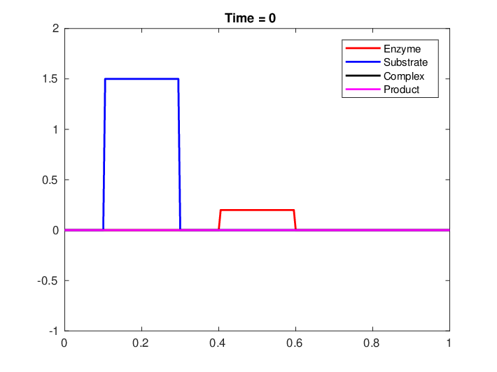
Refer to caption
(a) Initial concentrations
Refer to caption
(b) Concentrations at time t=10t=10.
Refer to caption
(c) Concentrations at time t=80t=80.
Refer to caption
(d) Concentrations at time t=200t=200.
Figure 1. The evolution of enzyme, complex and substrate in the case where (1.9) is not fulfilled.

We end the main body of our work with a numerical simulation, which can be seen in Fig. 1, that depicts the case where c0≡0c_{0}\equiv 0, e0e_{0} is not bounded away from zero, and supp​e0∩supp​s0=∅\mathrm{supp}e_{0}\cap\mathrm{supp}s_{0}=\emptyset. More precisely, we consider

Ω=(0,1),kf=100,kr=kc=1,de=dc=0,ds=dp=0.02,\Omega=(0,1),\;k_{f}=100,\;k_{r}=k_{c}=1,\;d_{e}=d_{c}=0,\;d_{s}=d_{p}=0.02,
e0(x)=0.2χ(0.4,0.6)(x),s0(x)=1.5χ(0.1,0.3), and c0(x)=p0(x)=0.e_{0}(x)=0.2\chi_{(0.4,0.6)}(x),\quad s_{0}(x)=1.5\chi_{(0.1,0.3)},\quad\text{ and }\quad c_{0}(x)=p_{0}(x)=0.

Under these assumptions we see that the equilibrium is given by

e∞​(x)=0.2​χ(0.4,0.6)​(x),s∞=c∞=0,p∞=0.3.e_{\infty}(x)=0.2\chi_{(0.4,0.6)}(x),\quad s_{\infty}=c_{\infty}=0,\quad p_{\infty}=0.3.

As expected, we see in Figure 1(B) that when the substrate ss diffuses to the region where the enzyme concentration is non-zero, it gets converted into the complex, which subsequently produces the product. This procedure continues to dissolve the substrate, as seen in Figure 1(C), and eventually converts it completely to the product, while the enzyme returns to its initial configuration in Figure 1(D).

Acknowledgment

The authors would like to thank Phillippe Laurençot for pointing out a mistake in the proof of Lemma 3.3.

Appendix A Additional Proofs

In this appendix we will show the proofs of several results which we elected to defer in order to not disrupt the flow of the presented work.

Lemma A.1.

Let Ω\Omega be a bounded domain with C1C^{1} boundary and assume that f∈W1,p​(Ω)f\in W^{1,p}\left(\Omega\right) for some p∈[1,∞)p\in[1,\infty) and g∈W2,p′​(Ω)g\in W^{2,p^{\prime}}\left(\Omega\right) where pp and p′p^{\prime} are Hölder conjugated. Then if ∇g​(x)⋅𝓃​(x)=0\nabla g(x)\cdot\mathcal{n}(x)=0, where 𝓃⁡(x)\mathcal{n}(x) is the outer normal to Ω\Omega at the point x∈∂Ωx\in\partial\Omega, we have that

(A.1) ∫Ωf(x)Δg(x)dx=−∫Ω∇f(x)⋅∇g(x)dx.\int_{\Omega}f(x)\Delta g(x)dx=-\int_{\Omega}\nabla f(x)\cdot\nabla g(x)dx.

Moreover, for any c∈ℝc\in\mathbb{R} we have that max⁡(f⁡(x),c)∈W1,p​(Ω)\max\left(f(x),c\right)\in W^{1,p}\left(\Omega\right) with

(A.2) ∇max⁡(f⁡(x),c)={∇f​(x)f⁡(x)>c0f⁡(x)≤c.\nabla\max\left(f(x),c\right)=\begin{cases}\nabla f(x)&f(x)>c\\ 0&f(x)\leq c\end{cases}.

and

(A.3) ∫Ωmax(f(x),c)Δg(x)dx=−∫{x|f⁡(x)≥c}∇f(x)⋅∇g(x)dx=−∫{x|f⁡(x)>c}∇f(x)⋅∇g(x)dx.\int_{\Omega}\max\left(f(x),c\right)\Delta g(x)dx=-\int_{\left\{x\;|\;f(x)\geq c\right\}}\nabla f(x)\cdot\nabla g(x)dx=-\int_{\left\{x\;|\;f(x)>c\right\}}\nabla f(x)\cdot\nabla g(x)dx.
Remark A.2.

The normal derivative of gg, ∇g​(x)⋅𝓃​(x)\nabla g(x)\cdot\mathcal{n}(x) on ∂Ω\partial\Omega is indeed well defined. This follows from a standard Trace theorem that states that when UU is a bounded open set with C1C^{1} boundary there exists a linear operator

T:W1,p​(U)→Lp​(∂U)T:W^{1,p}\left(U\right)\to L^{p}\left(\partial U\right)

such that

T​u=u|∂U, when ​u∈W1,p​(U)∩C⁡(U¯)Tu=u|_{\partial U},\qquad\text{ when }u\in W^{1,p}\left(U\right)\cap C\left(\overline{U}\right)

and

‖T​u‖Lp​(U)≤C​‖u‖W1,p​(U),\left\lVert Tu\right\rVert_{L^{p}\left(U\right)}\leq C\left\lVert u\right\rVert_{W^{1,p}\left(U\right)},

for some fixed geometric constant C>0C>0. A proof can be found in [Eva10, Theorem 1, pp. 272].
The expression ∇g​(x)⋅𝓃​(x)\nabla g(x)\cdot\mathcal{n}(x) on ∂Ω\partial\Omega is to be understood as T​(∇g​(x))⋅𝓃​(x)T\left(\nabla g(x)\right)\cdot\mathcal{n}(x).

Proof.

We start by noticing that for any f,g∈C∞​(Ω)f,g\in C^{\infty}\left(\Omega\right) we have that

(A.4) ∫Ωf(x)Δg(x)dx=∫∂Ωf(x)∇g(x)⋅𝓃(x)dx−∫Ω∇f(x)⋅∇g(x)dx,\int_{\Omega}f(x)\Delta g(x)dx=\int_{\partial\Omega}f(x)\nabla g(x)\cdot\mathcal{n}(x)dx-\int_{\Omega}\nabla f(x)\cdot\nabla g(x)dx,

by a simple integration by parts. Since any function in Wm,p​(Ω)W^{m,p}\left(\Omega\right) can be approximated by a C∞​(Ω¯)C^{\infty}\left(\overline{\Omega}\right) sequence in the Wm,p​(Ω)W^{m,p}\left(\Omega\right) norm (see [Eva10], for instance) we can find a sequence of C∞​(Ω¯)C^{\infty}\left(\overline{\Omega}\right) functions, {fn}n∈ℕ\left\{f_{n}\right\}_{n\in\mathbb{N}} and {gn}n∈ℕ\left\{g_{n}\right\}_{n\in\mathbb{N}}, such that

‖fn−f‖W1,p​(Ω)​⟶n→∞​0,‖gn−g‖W2,p′​(Ω)​⟶n→∞​0,\left\lVert f_{n}-f\right\rVert_{W^{1,p}\left(\Omega\right)}\underset{n\to\infty}{\longrightarrow}0,\qquad\left\lVert g_{n}-g\right\rVert_{W^{2,p^{\prime}}\left(\Omega\right)}\underset{n\to\infty}{\longrightarrow}0,

from which we immediately deduce that

(A.5) limn→∞∫Ωfn​(x)​Δ​gn​(x)​dx=∫Ωf⁡(x)​Δ​g​(x)​dx,limn→∞∫Ω∇fn​(x)⋅∇gn​(x)​dx=∫Ω∇f​(x)⋅∇g​(x)​dx.\begin{gathered}\lim_{n\to\infty}\int_{\Omega}f_{n}(x)\Delta g_{n}(x)dx=\int_{\Omega}f(x)\Delta g(x)dx,\\ \lim_{n\to\infty}\int_{\Omega}\nabla f_{n}(x)\cdot\nabla g_{n}(x)dx=\int_{\Omega}\nabla f(x)\cdot\nabla g(x)dx.\end{gathered}

Using the standard Trace theorem, mentioned in Remark A.2, we see that the traces of ff and ∇g\nabla g, T⁡(f)T\left(f\right) and T⁡(∇g)T\left(\nabla g\right) (to be thought of as a vector whose components are TT of the partial derivatives of gg), are well defined on ∂Ω\partial\Omega and

‖fn−T⁡(f)‖Lp​(∂Ω)=‖T⁡(fn−f)‖Lp​(∂Ω)≤C​‖fn−f‖W1,p​(Ω)​⟶n→∞​0\left\lVert f_{n}-T(f)\right\rVert_{L^{p}\left(\partial\Omega\right)}=\left\lVert T\left(f_{n}-f\right)\right\rVert_{L^{p}\left(\partial\Omega\right)}\leq C\left\lVert f_{n}-f\right\rVert_{W^{1,p}\left(\Omega\right)}\underset{n\to\infty}{\longrightarrow}0

and

‖∇gn−T⁡(∇g)‖Lp′​(∂Ω)=‖T⁡(∇gn−∇g)‖Lp​(∂Ω)≤C​‖gn−g‖W2,p′​(Ω)​⟶n→∞​0.\left\lVert\nabla g_{n}-T(\nabla g)\right\rVert_{L^{p^{\prime}}\left(\partial\Omega\right)}=\left\lVert T\left(\nabla g_{n}-\nabla g\right)\right\rVert_{L^{p}\left(\partial\Omega\right)}\leq C\left\lVert g_{n}-g\right\rVert_{W^{2,p^{\prime}}\left(\Omega\right)}\underset{n\to\infty}{\longrightarrow}0.

As such, using the Neumann boundary condition, we find that

(A.6) ‖∇gn​(x)⋅𝓃⁡(x)‖Lp′​(∂Ω)=‖(T⁡(∇gn​(x))−T⁡(∇g​(x)))⋅𝓃⁡(x)‖Lp′​(∂Ω)≤‖𝓃‖L∞​(∂Ω)​‖T⁡(∇gn​(x)−∇g​(x))‖Lp′​(∂Ω)​⟶n→∞​0\begin{gathered}\left\lVert\nabla g_{n}(x)\cdot\mathcal{n}(x)\right\rVert_{L^{p^{\prime}}\left(\partial\Omega\right)}=\left\lVert\left(T\left(\nabla g_{n}(x)\right)-T\left(\nabla g(x)\right)\right)\cdot\mathcal{n}(x)\right\rVert_{L^{p^{\prime}}\left(\partial\Omega\right)}\\ \leq\left\lVert\mathcal{n}\right\rVert_{L^{\infty}\left(\partial\Omega\right)}\left\lVert T\left(\nabla g_{n}(x)-\nabla g(x)\right)\right\rVert_{L^{p^{\prime}}\left(\partial\Omega\right)}\underset{n\to\infty}{\longrightarrow}0\end{gathered}

which implies that

(A.7) limn→∞∫∂Ωfn(x)∇gn(x)⋅𝓃(x)dx=0.\lim_{n\to\infty}\int_{\partial\Omega}f_{n}(x)\nabla g_{n}(x)\cdot\mathcal{n}(x)dx=0.

Combining (A.4), (A.5) and (A.7) gives us (A.1).

The facts that max⁡(f⁡(x),c)\max\left(f(x),c\right) belongs to W1,p​(Ω)W^{1,p}\left(\Omega\right) and that its derivative is given by (A.2) follow from Corollary 6.18 and the discussion that follows in [LL01]. Combining the above with the fact that any function f∈W1,p​(Ω)⊂Wloc1,1​(Ω)f\in W^{1,p}\left(\Omega\right)\subset W^{1,1}_{\mathrm{loc}}\left(\Omega\right) satisfies that ∇f​(x)=0\nabla f(x)=0 for almost every xx in f−1​({c})={x|f⁡(x)=c}f^{-1}\left(\left\{c\right\}\right)=\left\{x\;|\;f(x)=c\right\}, which can be found in Theorem 6.19 in [LL01], we see that

∇max⁡(f⁡(x),c)={∇f​(x)f⁡(x)≥c0f⁡(x)<c.\nabla\max\left(f(x),c\right)=\begin{cases}\nabla f(x)&f(x)\geq c\\ 0&f(x)<c\end{cases}.

and together with (A.1) and (A.2) we conclude (A.3). ∎

Next we turn our attention to the proof of Theorem 3.2, which requires the following lemma:

Lemma A.3.

Assume that Ω⊂ℝn\Omega\subset\mathbb{R}^{n}, n≥1n\geq 1, is a bounded, open domain with C2+ζ,ζ>0C^{2+\zeta},\zeta>0, boundary. Assume that d,T>0d,T>0, u0∈L∞​(Ω)u_{0}\in L^{\infty}(\Omega) and that the function ff belongs to Lq​(0,T,Lq​(Ω))L^{q}{(0,T;L^{q}(\Omega))} for all q∈[2,∞)q\in[2,\infty). Let

(A.8) u⁡(x,t)=ed​Δ​t​u0​(x)+∫0ted​Δ​(t−ξ)​f​(x,ξ)​𝑑ξ,u(x,t)=e^{d\Delta t}u_{0}(x)+\int_{0}^{t}e^{d\Delta(t-\xi)}f(x,\xi)d\xi,

where ed​Δ​te^{d\Delta t} is the semigroup generated by the operator d​Δd\Delta with homogeneous Neumann boundary conditions on Lq​(Ω)L^{q}(\Omega). Then uu is a strong solution to

(A.9) {∂tu⁡(x,t)−d​Δ​u​(x,t)=f⁡(x,t)x∈Ω,t∈(0,T)u​(x,0)=u0​(x)x∈Ω∂νu⁡(x,t)=0,x∈∂Ω,t∈(0,T).\begin{cases}\partial_{t}u(x,t)-d\Delta u(x,t)=f(x,t)&x\in\Omega,\;t\in(0,T)\\ u(x,0)=u_{0}(x)&x\in\Omega\\ \partial_{\nu}u(x,t)=0,&x\in\partial\Omega,t\in(0,T).\end{cases}
Proof.

Denoting by

u2​(x,t)=∫0ted​Δ​(t−ξ)​f​(x,ξ)​𝑑ξu_{2}(x,t)=\int_{0}^{t}e^{d\Delta(t-\xi)}f(x,\xi)d\xi

we see, according to [PS16, Theorem 6.2.3], that for any q∈[2,∞)q\in[2,\infty) we have that

u2∈Lq​((0,T),W2,q​(Ω))∩W1,q​((0,T),Lq​(Ω)).u_{2}\in L^{q}((0,T);W^{2,q}(\Omega))\cap W^{1,q}((0,T);L^{q}(\Omega)).

In particular, this implies that u2∈C0​([0,T],Lq​(Ω))u_{2}\in C^{0}([0,T];L^{q}(\Omega)), and u2u_{2} is a strong solution to (A.9) with u0≡0u_{0}\equiv 0.
To consider the general case we notice that we can’t use the same considerations for

u1​(x,t)=ed​Δ​t​u0​(x)u_{1}(x,t)=e^{d\Delta t}u_{0}(x)

as u0u_{0} does not necessarily belong to the right trace space. However, for every t>0t>0, we can use the regularisation properties of the semigroup to conclude that u1u_{1} belongs to the space C0​([0,T],Lq​(Ω))∩C1​((0,T],Lq​(Ω))C^{0}([0,T];L^{q}(\Omega))\cap C^{1}((0,T];L^{q}(\Omega)) and OPENu1​(⋅,t)∈W2,q​(Ω))u_{1}(\cdot,t)\in W^{2,q}(\Omega)) for all positive tt. This entails that u1u_{1} is continuous with respect to Lq​(Ω)L^{q}(\Omega) and belongs to Lq((τ,T);W2,q(Ω)])∩W1,q((τ,T);Lq(Ω))L^{q}((\tau,T);W^{2,q}(\Omega)])\cap W^{1,q}((\tau,T);L^{q}(\Omega)) for every τ>0\tau>0 and q∈[2,∞)q\in[2,\infty). As a consequence, we obtain that u1u_{1} is absolutely continuous as a Lq​(Ω)L^{q}(\Omega) valued function for positive times and is a strong solution to (A.9) with f≡0f\equiv 0. As u=u1+u2u=u_{1}+u_{2} we conclude the desired result. ∎

Proof of Theorem 3.2.

The proof is based on a standard fixed point argument. For a fixed T>0T>0 we denote by

𝒳\displaystyle\mathcal{X} ={(e,s,c,p)∈(L∞([0,T];L∞(Ω)))4|(e(0),s(0),c(0),p(0))=(e0,s0,c0,p0),\displaystyle=\bigg\{\left(e,s,c,p\right)\in\left({\color[rgb]{0,0,0}L^{\infty}}([0,T];L^{\infty}(\Omega))\right)^{4}\;|\;(e(0),s(0),c(0),p(0))=(e_{0},s_{0},c_{0},p_{0}),
 and ∥(e,s,c,p)∥(L∞​([0,T],L∞​(Ω)))4≤∥(e0,s0,c0,p0)∥L∞​(Ω)+1:=M},\displaystyle\qquad\text{ and }\quad\|(e,s,c,p)\|_{({\color[rgb]{0,0,0}L^{\infty}}([0,T];L^{\infty}(\Omega)))^{4}}\leq\|(e_{0},s_{0},c_{0},p_{0})\|_{L^{\infty}(\Omega)}+1:=M\bigg\},

where

‖(f1,f2,f3,f4)‖(L∞​([0,T],L∞​(Ω)))4=supt∈[0,T]∑i=14‖fi‖L∞​(Ω).\left\lVert\left(f_{1},f_{2},f_{3},f_{4}\right)\right\rVert_{({\color[rgb]{0,0,0}L^{\infty}}([0,T];L^{\infty}(\Omega)))^{4}}=\sup_{t\in[0,T]}\sum_{i=1}^{4}\left\lVert f_{i}\right\rVert_{L^{\infty}(\Omega)}.

We define a map ℱ\mathcal{F} and 𝒢\mathcal{G} on 𝒳\mathcal{X} by

ℱ⁡(e,s,c,p)​(x,t):=\displaystyle\mathcal{F}(e,s,c,p)(x,t):= (e0​(x)+∫0t(−kf​e​(x,ξ)​s​(x,ξ)+(kr+kc)​c​(x,ξ))​𝑑ξCLOSE,\displaystyle\left(e_{0}(x)+\int_{0}^{t}\left(-k_{f}e(x,\xi)s(x,\xi)+(k_{r}+k_{c})c(x,\xi)\right)d\xi,\right.
eds​Δ​t​s0​(x)+∫0teds​Δ​(t−ξ)​(−kf​e​(x,ξ)​s​(x,ξ)+kr​c​(x,ξ))​𝑑ξ,\displaystyle\quad e^{d_{s}\Delta t}s_{0}(x)+\int_{0}^{t}e^{d_{s}\Delta(t-\xi)}\left(-k_{f}e(x,\xi)s(x,\xi)+k_{r}c(x,\xi)\right)d\xi,
c0​(x)+∫0t(kf​e​(x,ξ)​s​(x,ξ)−(kr+kc)​c​(x,ξ))​𝑑ξ,\displaystyle\quad c_{0}(x)+\int_{0}^{t}\left(k_{f}e(x,\xi)s(x,\xi)-(k_{r}+k_{c})c(x,\xi)\right)d\xi,
OPENedp​Δ​t​p0​(x)+∫0tedp​Δ​(t−ξ)​kc​c​(x,ξ)​𝑑ξ),\displaystyle\quad\left.e^{d_{p}\Delta t}p_{0}(x)+\int_{0}^{t}e^{d_{p}\Delta(t-\xi)}k_{c}c(x,\xi)d\xi\right),

and

𝒢⁡(e,s,c,p)​(x,t):=ℱ⁡(e+,s+,c+,p+)​(x,t),\displaystyle\mathcal{G}(e,s,c,p)(x,t):=\ \mathcal{F}(e_{+},s_{+},c_{+},p_{+})(x,t),

and where

f+:=max⁡(f,0).f_{+}:=\max\left(f,0\right).

We will now show that for TT small enough, ℱ\mathcal{F} is a contraction mapping from 𝒳\mathcal{X} into 𝒳\mathcal{X}. This will show the existence of a unique bounded strong solution, at least on (0,T)(0,T). Moreover, by showing that 𝒢\mathcal{G} is also a contraction mapping 𝒳\mathcal{X} into 𝒳\mathcal{X} admitting fixed point such that e,s,ce,s,c and pp are non-negative, we would be able conclude that this fixed point is in fact a fixed point for ℱ\mathcal{F}, and as such the strong solution we have found is in fact non-negative.

Clearly, ℱ⁡(e,s,c,p)​(0)=𝒢⁡(e,s,c,p)​(0)=(e0,s0,c0,p0)\mathcal{F}(e,s,c,p)(0)=\mathcal{G}(e,s,c,p)(0)=(e_{0},s_{0},c_{0},p_{0}). Moreover, since

(A.10) ‖ed​Δ​t​f‖L∞​(Ω)≤‖f‖L∞​(Ω)\|e^{d\Delta t}f\|_{L^{\infty}(\Omega)}\leq\|f\|_{L^{\infty}(\Omega)}

and

(A.11) ‖f+‖L∞​(Ω)≤‖f‖L∞​(Ω)\left\lVert f_{+}\right\rVert_{L^{\infty}(\Omega)}\leq\left\lVert f\right\rVert_{L^{\infty}(\Omega)}

we see that

‖ℱ⁡(e,s,c,p)‖(L∞​([0,T],L∞​(Ω)))4≤‖(e0,s0,c0,p0)‖L∞​(Ω)+𝒞0​(M2+1)​T\displaystyle\|\mathcal{F}(e,s,c,p)\|_{({\color[rgb]{0,0,0}L^{\infty}}([0,T];L^{\infty}(\Omega)))^{4}}\leq\|(e_{0},s_{0},c_{0},p_{0})\|_{L^{\infty}(\Omega)}+\mathcal{C}_{0}\left(M^{2}+1\right)T

and

‖𝒢⁡(e,s,c,p)‖(L∞​([0,T],L∞​(Ω)))4≤‖(e0,s0,c0,p0)‖L∞​(Ω)+𝒞0​(M2+1)​T\displaystyle\|\mathcal{G}(e,s,c,p)\|_{({\color[rgb]{0,0,0}L^{\infty}}([0,T];L^{\infty}(\Omega)))^{4}}\leq\|(e_{0},s_{0},c_{0},p_{0})\|_{L^{\infty}(\Omega)}+\mathcal{C}_{0}\left(M^{2}+1\right)T

for some constant 𝒞0\mathcal{C}_{0} that depends is independent of MM and TT. Choosing TT small enough so that

𝒞0​(M2+1)​T≤1\mathcal{C}_{0}(M^{2}+1)T\leq 1

we conclude that ℱ\mathcal{F} and 𝒢\mathcal{G} map 𝒳\mathcal{X} into 𝒳\mathcal{X} itself.

Next, using (A.10) again, we find that

‖ℱ⁡(e1,s1,c1,p1)−ℱ⁡(e2,s2,c2,p2)‖(L∞​([0,T],L∞​(Ω)))4\displaystyle\|\mathcal{F}(e_{1},s_{1},c_{1},p_{1})-\mathcal{F}(e_{2},s_{2},c_{2},p_{2})\|_{\left({\color[rgb]{0,0,0}L^{\infty}}([0,T];L^{\infty}(\Omega))\right)^{4}}
≤∫0T‖−kf​(e1​(ξ)​s1​(ξ)−e2​(ξ)​s2​(ξ))+(kr+kc)​(c1​(ξ)−c2​(ξ))‖L∞​(Ω)​𝑑ξ\displaystyle\leq\int_{0}^{T}\left\|-k_{f}\left(e_{1}\left(\xi\right)s_{1}\left(\xi\right)-e_{2}\left(\xi\right)s_{2}\left(\xi\right)\right)+(k_{r}+k_{c})\left(c_{1}\left(\xi\right)-c_{2}\left(\xi\right)\right)\right\|_{L^{\infty}(\Omega)}d\xi
+∫0T‖−kf(e1(ξ)s1(ξ)−e2(ξ)s2(ξ))+kr(c1(ξ)−c2(ξ))‖L∞​(Ω)dξ\displaystyle\quad+\int_{0}^{T}\left\|-k_{f}\left(e_{1}\left(\xi\right)s_{1}\left(\xi\right)-e_{2}\left(\xi\right)s_{2}\left(\xi\right)\right)+k_{r}\left(c_{1}\left(\xi\right)-c_{2}\left(\xi\right)\right)\right\|_{L^{\infty}(\Omega)}d\xi
+∫0T‖kf(e1s1(ξ)−e2(ξ)s2(ξ))−(kr+kc)(c1(ξ)−c2(ξ))‖L∞​(Ω)dξ\displaystyle\quad+\int_{0}^{T}\left\|k_{f}\left(e_{1}s_{1}\left(\xi\right)-e_{2}\left(\xi\right)s_{2}\left(\xi\right)\right)-(k_{r}+k_{c})\left(c_{1}\left(\xi\right)-c_{2}\left(\xi\right)\right)\right\|_{L^{\infty}(\Omega)}d\xi
+∫0T‖kc(c1(ξ)−c2(ξ))‖L∞​(Ω)dξ\displaystyle\quad+\int_{0}^{T}\left\|k_{c}\left(c_{1}\left(\xi\right)-c_{2}\left(\xi\right)\right)\right\|_{L^{\infty}(\Omega)}d\xi
≤𝒞1​(M+1)​T​‖(e1,s1,c1,p1)−(e2,s2,c2,p2)‖(L∞​([0,T],L∞​(Ω)))4\displaystyle\leq\mathcal{C}_{1}(M+1)T\left\|\left(e_{1},s_{1},c_{1},p_{1})-(e_{2},s_{2},c_{2},p_{2}\right)\right\|_{({\color[rgb]{0,0,0}L^{\infty}}([0,T];L^{\infty}(\Omega)))^{4}}
and
‖𝒢⁡(e1,s1,c1,p1)−𝒢⁡(e2,s2,c2,p2)‖(L∞​([0,T],L∞​(Ω)))4\displaystyle\|\mathcal{G}(e_{1},s_{1},c_{1},p_{1})-\mathcal{G}(e_{2},s_{2},c_{2},p_{2})\|_{\left({\color[rgb]{0,0,0}L^{\infty}}([0,T];L^{\infty}(\Omega))\right)^{4}}
=\displaystyle= ‖ℱ⁡(e1+,s1+,c1+,p1+)−ℱ⁡(e2+,s2+,c2+,p2+)‖(L∞​([0,T],L∞​(Ω)))4\displaystyle\|\mathcal{F}(e_{1+},s_{1+},c_{1+},p_{1+})-{\color[rgb]{0,0,0}\mathcal{F}}(e_{2+},s_{2+},c_{2+},p_{2+})\|_{\left({\color[rgb]{0,0,0}L^{\infty}}([0,T];L^{\infty}(\Omega))\right)^{4}}
≤𝒞1​(M+1)​T​‖(e1,s1,c1,p1)−(e2,s2,c2,p2)‖(L∞​([0,T],L∞​(Ω)))4\displaystyle\leq\mathcal{C}_{1}(M+1)T\left\|(e_{1},s_{1},c_{1},p_{1})-(e_{2},s_{2},c_{2},p_{2})\right\|_{({\color[rgb]{0,0,0}L^{\infty}}([0,T];L^{\infty}(\Omega)))^{4}}

for a constant 𝒞1\mathcal{C}_{1} that is independent of MM and TT, where we have used the elementary inequality

|a+−b+|≤|a−b|.|a_{+}-b_{+}|\leq|a-b|.

Restricting TT further so that

𝒞1​(M+1)​T<1\mathcal{C}_{1}(M+1)T<1

we see that ℱ\mathcal{F} and 𝒢\mathcal{G} are contraction mappings from 𝒳\mathcal{X} into 𝒳\mathcal{X}, and therefore they each have a unique fixed point. We denote by (e¯,s¯,c¯,p¯)(\overline{e},\overline{s},\overline{c},\overline{p}) the fixed point of 𝒢\mathcal{G}. According to Lemma A.3 it is a local strong solution to the system of equations1414 14 Note that by the definition of 𝒳\mathcal{X} and ℱ\mathcal{F}, the function ff from (A.8) is in L∞​([0,T],L∞​(Ω))L^{\infty}([0,T];L^{\infty}(\Omega)), and as such the conditions of the Lemma are satisfied.

(A.12) {∂te¯​(x,t)=−kf​e¯+​(x,t)​s¯+​(x,t)+(kr+kc)​c¯+​(x,t),x∈Ω,t>0,∂ts¯​(x,t)−ds​Δ​s¯​(x,t)=−kf​e¯+​(x,t)​s¯+​(x,t)+kr​c¯+​(x,t),x∈Ω,t>0,∂tc¯​(x,t)=kf​e¯+​(x,t)​s¯+​(x,t)−(kr+kc)​c¯+​(x,t),x∈Ω,t>0,∂tp¯​(x,t)−dp​Δ​p¯​(x,t)=kc​c¯+​(x,t),x∈Ω,t>0,∂νs⁡(x,t)=∂νp⁡(x,t)=0,x∈∂Ω,t>0,e(x,0)=e0(x),s(x,0)=s0(x),c(x,0)=c0(x),p(x,0)=p0(x),x∈Ω,\begin{cases}\partial_{t}\overline{e}(x,t)=-k_{f}\overline{e}_{+}(x,t)\overline{s}_{+}(x,t)+(k_{r}+k_{c})\overline{c}_{+}(x,t),&x\in\Omega,t>0,\\ \partial_{t}\overline{s}(x,t)-d_{s}\Delta\overline{s}(x,t)=-k_{f}\overline{e}_{+}(x,t)\overline{s}_{+}(x,t)+k_{r}\overline{c}_{+}(x,t),&x\in\Omega,t>0,\\ \partial_{t}\overline{c}(x,t)=k_{f}\overline{e}_{+}(x,t)\overline{s}_{+}(x,t)-(k_{r}+k_{c})\overline{c}_{+}(x,t),&x\in\Omega,t>0,\\ \partial_{t}\overline{p}(x,t)-d_{p}\Delta\overline{p}(x,t)=k_{c}\overline{c}_{+}(x,t),&x\in\Omega,t>0,\\ \partial_{\nu}s(x,t)=\partial_{\nu}p(x,t)=0,&x\in\partial\Omega,t>0,\\ e(x,0)=e_{0}(x),\;s(x,0)=s_{0}(x),\;c(x,0)=c_{0}(x),\;p(x,0)=p_{0}(x),&x\in\Omega,\end{cases}

on (0,T)(0,T). Let TmaxT_{\mathrm{max}} be the maximal time of existence for the solution (e¯,s¯,c¯,p¯)(\overline{e},\overline{s},\overline{c},\overline{p}). To show that (e¯,s¯,c¯,p¯)(\overline{e},\overline{s},\overline{c},\overline{p}) is a global solution, i.e. Tmax=+∞T_{\mathrm{max}}=+\infty, it is enough to show that

(A.13) ‖(e¯,s¯,c¯,p¯)‖(L∞​([0,T],L∞​(Ω)))4≤C⁡(T){\color[rgb]{0,0,0}\left\lVert(\overline{e},\overline{s},\overline{c},\overline{p})\right\rVert}_{({\color[rgb]{0,0,0}L^{\infty}}([0,T];L^{\infty}(\Omega)))^{4}}\leq C(T)

for some continuous function C⁡(T):[0,∞)→[0,∞)C(T):[0,\infty)\to[0,\infty) (see, for instance, [Zhe04, Theorem 2.5.5]). The proof of the existence of such function is intertwined with the non-negativity property of (e¯,s¯,c¯,p¯)(\overline{e},\overline{s},\overline{c},\overline{p}), which will also show that (e¯,s¯,c¯,p¯)(\overline{e},\overline{s},\overline{c},\overline{p}) is in fact a solution to (1.2).

Denoting by f−=max⁡(0,−f)=(−f)+f_{-}=\max\left(0,-f\right)=\left(-f\right)_{+} the so-called negative part of ff, we notice that when ff is absolutely continuous with respect to tt so is f−f_{-}, and a.e. in tt

dd​t​f−2​(t)=2​f−​(t)​dd​t​f−​(t)=−2​f−​(t)​dd​t​f​(t).\frac{d}{dt}f^{2}_{-}(t)=2f_{-}(t)\frac{d}{dt}f_{-}(t)=-2f_{-}(t)\frac{d}{dt}f(t).

As such, if f⁡(x,t)f(x,t) is a strong solution to

(A.14) ∂tf⁡(x,t)−d​Δ​f​(x,t)=g⁡(t,x)−α⁡(x,t)​f+​(x,t)\partial_{t}f(x,t)-d\Delta f(x,t)=g(t,x)-\alpha(x,t)f_{+}(x,t)

where g⁡(x,t)g(x,t) and α⁡(x,t)\alpha(x,t) are non-negative functions, we see that by multiplying the above with −f−​(x,t)≤0-f_{-}(x,t)\leq 0, we find that

12​∂tf−2​(x,t)−d​Δ​f​(x,t)​f−​(x,t)=−g⁡(t,x)​f−​(x,t)≤0.\frac{1}{2}\partial_{t}f^{2}_{-}(x,t)-d\Delta f(x,t)f_{-}(x,t)=-g(t,x)f_{-}(x,t)\leq 0.

Integrating over Ω×(0,t)\Omega\times(0,t) gives1515 15 The appearance of the norm of ∇f−\nabla f_{-}, as well as its existence, is an immediate and simple variant of our discussion in Lemma A.1 in Appendix A. Moreover, according to the definition of the strong solutions we find that vv is absolutely continuous with respect to OPENL2​(Ω))L^{2}(\Omega)). As the L2​(Ω)L^{2}(\Omega) scalar product is bilinear and continuous, we can apply the product rule to find that dd​t​‖v⁡(t)‖L2​(Ω)2=dd​t​∫Ωv⁡(x,t)​v​(x,t)​𝑑x=2​∫Ω∂tv⁡(x,t)​v​(x,t)​𝑑x\frac{d}{dt}\left\lVert v(t)\right\rVert_{L^{2}(\Omega)}^{2}=\frac{d}{dt}\int_{\Omega}v(x,t)v(x,t)dx=2\int_{\Omega}\partial_{t}v(x,t)v(x,t)dx for almost all t>0t>0.

12​‖f−​(t)‖L2​(Ω)2+d​∫0t‖∇f−​(ξ)‖L2​(Ω)2​𝑑ξ≤12​‖f−​(0)‖L2​(Ω)2,\frac{1}{2}\left\lVert f_{-}(t)\right\rVert^{2}_{L^{2}(\Omega)}+d\int_{0}^{t}\left\lVert\nabla f_{-}(\xi)\right\rVert^{2}_{L^{2}(\Omega)}d\xi\leq\frac{1}{2}\left\lVert f_{-}(0)\right\rVert^{2}_{L^{2}(\Omega)},

which implies that if f⁡(0)f(0) is non-negative, i.e. f−​(0)≡0f_{-}(0)\equiv 0 (a.e in xx) then f−​(t)≡0f_{-}(t)\equiv 0 (a.e in xx) for any t>0t>0 for which ff is a strong solution to (A.14). As the equations for e¯\overline{e}, c¯\overline{c}, s¯\overline{s} and p¯\overline{p} are of the form (A.14), we conclude the non-negativity of e¯\overline{e}, c¯\overline{c}, s¯\overline{s} and p¯\overline{p}, and as such the fact that it is in fact a solution to (1.2).

Lastly, we shall show that (A.13) is valid for a constant function C⁡(T)C(T) which will show both the global existence and uniform boundedness, concluding the proof.
Indeed, using the definition strong solution (Duhamel’s formula, as is expressed in the definition of ℱ\mathcal{F}) and the non-negativity of e¯\overline{e} and c¯\overline{c} we see that

max⁡(|e¯​(x,t)|,|c¯​(x,t)|)=max⁡(e¯​(x,t),c¯​(x,t))≤e¯​(x,t)+c¯​(x,t)=‖e0‖L∞​(Ω)+‖c0‖L∞​(Ω).\max\left(\left\lvert\overline{e}(x,t)\right\rvert,\left\lvert\overline{c}(x,t)\right\rvert\right)=\max\left(\overline{e}(x,t),\overline{c}(x,t)\right)\leq\overline{e}(x,t)+\overline{c}(x,t)=\left\lVert e_{0}\right\rVert_{L^{\infty}(\Omega)}+\left\lVert c_{0}\right\rVert_{L^{\infty}(\Omega)}.

Thus, for any TT for which e¯\overline{e} and c¯\overline{c} are strong solutions to (1.2) we have that

(A.15) supt≤Tmax⁡(‖e¯​(t)‖L∞​(Ω),‖c¯​(t)‖L∞​(Ω))≤‖e0‖L∞​(Ω)+‖c0‖L∞​(Ω).\sup_{t\leq T}\max\left(\left\lVert\overline{e}(t)\right\rVert_{L^{\infty}(\Omega)},\left\lVert\overline{c}(t)\right\rVert_{L^{\infty}(\Omega)}\right)\leq\left\lVert e_{0}\right\rVert_{L^{\infty}(\Omega)}+\left\lVert c_{0}\right\rVert_{L^{\infty}(\Omega)}.

It remains to show the boundedness of s¯\overline{s} and p¯\overline{p}. Summing s¯​(t)\overline{s}(t), c¯​(t)\overline{c}(t), p¯​(t)\overline{p}(t), and integrating over gives

(A.16) ‖s¯​(t)‖L1​(Ω)+‖c¯​(t)‖L1​(Ω)+‖p¯​(t)‖L1​(Ω)=‖s0‖L1​(Ω)+‖c0‖L1​(Ω)+‖p0‖L1​(Ω)∀t≥0,\|\overline{s}(t)\|_{L^{1}(\Omega)}+\|\overline{c}(t)\|_{L^{1}(\Omega)}+\|\overline{p}(t)\|_{L^{1}(\Omega)}=\|s_{0}\|_{L^{1}(\Omega)}+\|c_{0}\|_{L^{1}(\Omega)}+\|p_{0}\|_{L^{1}(\Omega)}\quad\forall t\geq 0,

where we have used the non-negativity of the solution again. For any q≥2q\geq 2 we have

dd​t​‖s¯​(t)‖Lq​(Ω)q\displaystyle\frac{d}{dt}\|\overline{s}(t)\|_{L^{q}(\Omega)}^{q} =q​∫Ωs¯q−1​(x,t)​∂ts¯​(x,t)​𝑑x\displaystyle=q\int_{\Omega}\overline{s}^{q-1}(x,t)\partial_{t}\overline{s}(x,t)dx
≤−q(q−1)ds∫Ωs¯(x,t)q−2|∇s¯(x,t)|2dx+krq∫Ωs¯(x,t)q−1c¯(x,t)dx\displaystyle\leq-q(q-1)d_{s}\int_{\Omega}\overline{s}(x,t)^{q-2}|\nabla\overline{s}(x,t)|^{2}dx+k_{r}q\int_{\Omega}\overline{s}(x,t)^{q-1}\overline{c}(x,t)dx
≤−q(q−1)ds∫Ωs¯(x,t)q−2|∇s¯(x,t)|2dx+krq‖s¯(t)‖Lq​(Ω)q−1‖c¯(t)‖Lq​(Ω)\displaystyle\leq-q(q-1)d_{s}\int_{\Omega}\overline{s}(x,t)^{q-2}|\nabla\overline{s}(x,t)|^{2}dx+k_{r}q\left\lVert\overline{s}(t)\right\rVert^{q-1}_{L^{q}(\Omega)}\left\lVert\overline{c}(t)\right\rVert_{L^{q}(\Omega)}
≤−4​(q−1)​dsq∫Ω|∇(s¯(x,t)q2)|2dx+kr((q−1)∥s¯(t)∥Lq​(Ω)q+∥c¯(t)∥Lq​(Ω)q).\displaystyle\leq-\frac{4(q-1)d_{s}}{q}\int_{\Omega}\left|\nabla\left(\overline{s}(x,t)^{\frac{q}{2}}\right)\right|^{2}dx+k_{r}\left((q-1)\|\overline{s}(t)\|_{L^{q}(\Omega)}^{q}+\|\overline{c}(t)\|_{L^{q}(\Omega)}^{q}\right).

Using the uniform bound of c¯\overline{c} in (A.15) we find that

(A.17) dd​t​‖s¯​(t)‖Lq​(Ω)q+4​(q−1)​dsq​‖s¯​(t)q2‖H1​(Ω)2≤q​Cc0,e0​(‖s¯‖Lq​(Ω)q+1).\frac{d}{dt}\|\overline{s}(t)\|_{L^{q}(\Omega)}^{q}+\frac{4(q-1)d_{s}}{q}\left\lVert\overline{s}(t)^{\frac{q}{2}}\right\rVert_{H^{1}(\Omega)}^{2}\leq qC_{c_{0},e_{0}}\left(\|\overline{s}\|_{L^{q}(\Omega)}^{q}+1\right).

Thanks to the continuous Sobolev embedding H1​(Ω)↪Ln∗​(Ω)H^{1}(\Omega)\hookrightarrow L^{n^{*}}(\Omega) with

n∗={+∞ if ​n=1,<+∞​ arbitrary  if ​n=2,2​nn−2 if ​n≥3.n^{*}=\begin{cases}+\infty&\text{ if }n=1,\\ <+\infty\text{ arbitrary }&\text{ if }n=2,\\ \frac{2n}{n-2}&\text{ if }n\geq 3.\end{cases}

we find that

(A.18) ‖s¯q2‖H1​(Ω)2≥Cn​‖s¯q2‖Ln∗​(Ω)2=Cn​‖s¯‖Lq0​(Ω)q,\left\lVert\overline{s}^{\frac{q}{2}}\right\rVert_{H^{1}(\Omega)}^{2}\geq C_{n}\left\lVert\overline{s}^{\frac{q}{2}}\right\rVert_{L^{n^{\ast}}(\Omega)}^{2}=C_{n}\left\lVert\overline{s}\right\rVert_{L^{q_{0}}(\Omega)}^{q},

where q0=n∗​q2>qq_{0}=\frac{n^{\ast}q}{2}>q. Using the interpolation inequality

‖f‖Lq​(Ω)q≤‖f‖Lq0​(Ω)θ​q​‖f‖L1​(Ω)(1−θ)​q\left\lVert f\right\rVert_{L^{q}(\Omega)}^{q}\leq\left\lVert f\right\rVert_{L^{q_{0}}(\Omega)}^{\theta q}\left\lVert f\right\rVert_{L^{1}(\Omega)}^{\left(1-\theta\right)q}

where θ∈(0,1)\theta\in(0,1) satisfies 1q=θq0+1−θ1\frac{1}{q}=\frac{\theta}{q_{0}}+\frac{1-\theta}{1}, together with (A.16) we see that any ε>0\varepsilon>0 there exists a constant Cε>0C_{\varepsilon}>0 such that

(A.19) ‖s¯‖Lq​(Ω)q≤ε​‖s¯‖Lq0​(Ω)q+Cε.\|\overline{s}\|_{L^{q}(\Omega)}^{q}\leq\varepsilon\|\overline{s}\|_{L^{q_{0}}(\Omega)}^{q}+C_{\varepsilon}.

Combining (A.17), (A.18) and (A.19), we see that for any ε>0\varepsilon>0

dd​t​‖s¯​(t)‖Lq​(Ω)q+2​ds​Cn​‖s¯​(t)‖Lq​(Ω)q≤q​Cc0,e0​(ε​‖s¯‖Lq0​(Ω)q+Cε,),\frac{d}{dt}\|\overline{s}(t)\|_{L^{q}(\Omega)}^{q}+2d_{s}C_{n}\|\overline{s}(t)\|_{L^{q}(\Omega)}^{q}\leq qC_{c_{0},e_{0}}\left(\varepsilon\|\overline{s}\|_{L^{q_{0}}(\Omega)}^{q}+C_{\varepsilon,}\right),

from which we get with a choice of ε\varepsilon small enough1616 16 ε=ds​Cnq​Cc0,e0\varepsilon=\frac{d_{s}C_{n}}{qC_{c_{0},e_{0}}} will do that

(A.20) supt≥0‖s¯​(t)‖Lq​(Ω)<+∞\sup_{t\geq 0}\|\overline{s}(t)\|_{L^{q}(\Omega)}<+\infty

for any 2≤q<+∞2\leq q<+\infty. Applying a simple variant of Lemma 3.3 with δ=0\delta=0, where the L∞L^{\infty} bound is on [0,T2]\left[0,\frac{T}{2}\right] instead of [0,1][0,1], shows that1717 17 The appropriate ff in this case is f=−kf​e​s+kr​cf=-k_{f}es+k_{r}c whose LpL^{p} bound follows from the uniform L∞L^{\infty} bound on ee and cc and (A.20).

supt≥0‖s¯​(t)‖L∞​(Ω)<+∞.\sup_{t\geq 0}\|\overline{s}(t)\|_{L^{\infty}(\Omega)}<+\infty.

The uniform bound of p¯\overline{p} follows in the exact same way. ∎

We conclude the appendix with the proofs of lemmas 3.3 and 3.4.

Proof of Lemma 3.3.

A known estimate on the kernel of the heat equation (see for instance [Dav89, Theorem 3.2.9, page 90]) implies that the solution to the heat equation with homogeneous Neumann boundary condition and initial datum in Lp​(Ω)L^{p}\left(\Omega\right) satisfies

(A.21) ‖u⁡(t)‖L∞​(Ω)=‖ed​Δ​t​u0‖L∞​(Ω)≤Cd​t−n2​p​‖u0‖Lp​(Ω)∀0<t≤1,\left\lVert u(t)\right\rVert_{L^{\infty}(\Omega)}=\left\lVert e^{d\Delta t}u_{0}\right\rVert_{L^{\infty}(\Omega)}\leq C_{d}t^{-\frac{n}{2p}}\left\lVert u_{0}\right\rVert_{L^{p}(\Omega)}\quad\forall{\color[rgb]{1,0,0}0<t\leq 1},

for some fixed known constant that depends on Ω\Omega and the diffusion coefficient dd1818 18 One can easily extent (A.21) to 0<t<T0<t<T for any given T>0T>0. The constant CdC_{d} in that case will become dependent on TT (and one should denote it by Cd,TC_{d,T}).. As such, a solution to the equation

{∂tu⁡(x,t)−d​Δ​u​(x,t)=f⁡(x,t)x∈Ω,t>0u⁡(x,0)=0x∈Ω∂νu⁡(x,t)=0,x∈∂Ω,t>0,\begin{cases}\partial_{t}u(x,t)-d\Delta u(x,t)=f(x,t)&x\in\Omega,\;t>0\\ u(x,0)=0&x\in\Omega\\ \partial_{\nu}u(x,t)=0,&x\in\partial\Omega,t>0,\end{cases}

would satisfy, according to the Duhamel formula,

u⁡(x,t+1)=ed​Δ​u​(x,t)+∫01e−d​Δ​s​f​(x,t+s)​𝑑s,t>0u(x,t+1)=e^{d\Delta}u(x,t)+\int_{0}^{1}e^{-d\Delta s}f(x,t+s)ds,\quad t>0

which, together with (A.21), implies that

‖u⁡(t+1)‖L∞​(Ω)≤Cd​(‖u⁡(t)‖Lp​(Ω)+∫01(1+s−n2​p)​‖f⁡(t+s)‖Lp​(Ω)​𝑑s).\left\lVert u(t+1)\right\rVert_{L^{\infty}(\Omega)}\leq C_{d}\left(\left\lVert u(t)\right\rVert_{L^{p}(\Omega)}+\int_{0}^{1}\left(1+s^{-\frac{n}{2p}}\right)\left\lVert f(t+s)\right\rVert_{L^{p}(\Omega)}ds\right).

Using conditions (3.1) we find that

‖u⁡(t+1)‖L∞​(Ω)≤𝒞​Cd​(1+∫01(1+s−n2​p)​e−δ​s​𝑑s)​e−δ​t.\left\lVert u(t+1)\right\rVert_{L^{\infty}(\Omega)}\leq\mathcal{C}C_{d}\left(1+\int_{0}^{1}\left(1+s^{-\frac{n}{2p}}\right)e^{-\delta s}ds\right)e^{-\delta t}.

If p>n2p>\frac{n}{2} then

∫01s−n2​p​e−δ​s​𝑑s≤∫01s−n2​p​𝑑s=Cn,p<∞,\int_{0}^{1}s^{-\frac{n}{2p}}e^{-\delta s}ds\leq\int_{0}^{1}s^{-\frac{n}{2p}}ds=C_{n,p}<\infty,

and we conclude that for all t≥1t\geq 1

‖u⁡(t)‖L∞​(Ω)≤𝒞​Cd​(2+Cn,p)​e−δ⁡(t−1).\left\lVert u(t)\right\rVert_{L^{\infty}(\Omega)}\leq\mathcal{C}C_{d}\left(2+C_{n,p}\right)e^{-\delta(t-1)}.

As for any t∈[0,1]t\in[0,1] we have that

supt∈[0,1]‖u⁡(t)‖L∞​(Ω)≤𝒮≤𝒮​eδ​e−δ​t\sup_{t\in[0,1]}\left\lVert u(t)\right\rVert_{L^{\infty}(\Omega)}\leq\mathcal{S}\leq\mathcal{S}e^{\delta}e^{-\delta t}

due to (3.1), we find that

‖u⁡(t)‖L∞​(Ω)≤eδ​max⁡(𝒮,𝒞​Cd​(2+Cn,p))​e−δ​t,\left\lVert u(t)\right\rVert_{L^{\infty}(\Omega)}\leq e^{\delta}\max\left(\mathcal{S},\mathcal{C}C_{d}\left(2+C_{n,p}\right)\right)e^{-\delta t},

which is the desired result. ∎

Proof of Lemma 3.4.

Defining the function v⁡(x,t)=u⁡(x,t)−u¯​(t)v(x,t)=u(x,t)-\overline{u}(t) we find that vv solves the equation

{∂tv⁡(x,t)−d​Δ​v​(x,t)=f⁡(x,t)−∂tu¯​(t)x∈Ω,t>0u⁡(x,0)=u0​(x)−u0¯x∈Ω∂νu⁡(x,t)=0,x∈∂Ω.t>0.\begin{cases}\partial_{t}v(x,t)-d\Delta v(x,t)=f(x,t)-\partial_{t}\overline{u}(t)&x\in\Omega,\;t>0\\ u(x,0)=u_{0}(x)-\overline{u_{0}}&x\in\Omega\\ \partial_{\nu}u(x,t)=0,&x\in\partial\Omega.t>0.\end{cases}

Denoting by f~​(x,t)=f⁡(x,t)−∂tu¯​(t)\widetilde{f}(x,t)=f(x,t)-\partial_{t}\overline{u}(t), multiplying the first line of the equation by v⁡(x,t)v(x,t) and integrating over the domain yields the equality

∂t‖v⁡(t)‖L2​(Ω)2=−2​d​‖∇v​(x,t)‖L2​(Ω)2+2​∫Ωf~​(x,t)​v​(x,t)​𝑑x.\partial_{t}\left\lVert v(t)\right\rVert_{L^{2}(\Omega)}^{2}=-2d\left\lVert\nabla v(x,t)\right\rVert_{L^{2}(\Omega)}^{2}+2\int_{\Omega}\widetilde{f}(x,t)v(x,t)dx.

Thus, using the Poincaré inequality (3.4) and the fact that v¯​(t)=0\overline{v}(t)=0 we find that

∂t‖v⁡(t)‖L2​(Ω)2≤−2​dCP​‖v⁡(t)‖L2​(Ω)2+2​‖f~​(t)‖L2​(Ω)​‖v⁡(t)‖L2​(Ω)\partial_{t}\left\lVert v(t)\right\rVert_{L^{2}(\Omega)}^{2}\leq-\frac{2d}{C_{P}}\left\lVert v(t)\right\rVert_{L^{2}(\Omega)}^{2}+2\left\lVert\widetilde{f}(t)\right\rVert_{L^{2}(\Omega)}\left\lVert v(t)\right\rVert_{L^{2}(\Omega)}
≤−2​dCP​(1−ε)​‖v⁡(t)‖L2​(Ω)2+CP​‖f~​(t)‖L2​(Ω)22​d​ε,\leq-\frac{2d}{C_{P}}\left(1-\varepsilon\right)\left\lVert v(t)\right\rVert_{L^{2}(\Omega)}^{2}+\frac{C_{P}\left\lVert\widetilde{f}(t)\right\rVert_{L^{2}(\Omega)}^{2}}{2d\varepsilon},

where we have used the fact that for any δ>0\delta>0 and a,b≥0a,b\geq 0

2​a​b≤δ​a2+b2δ2ab\leq\delta a^{2}+\frac{b^{2}}{\delta}

and chose δ=2​d​εCP\delta=\frac{2d\varepsilon}{C_{P}}. The result follows from a simple integration and the fact that by integrating our heat equation over Ω\Omega we find that

∂tu¯​(t)=∫Ωf⁡(x,t)​𝑑x=f¯​(t).\partial_{t}\overline{u}(t)=\int_{\Omega}f(x,t)dx=\overline{f}(t).

∎

References

  • [AMTU01] Anton Arnold, Peter Markowich, Giuseppe Toscani, and Andreas Unterreiter. On convex sobolev inequalities and the rate of convergence to equilibrium for fokker-planck type equations. Communications in Partial Differential Equations, 26:43–100, 2001.
  • [BRZ20] Marcel Braukhoff, Claudia Raithel, and Nicola Zamponi. Partial hölder regularity for bounded solutions of a class of cross-diffusion systems with entropy structure. Preprint, 2020.
  • [Dav89] E. B. Davies. Heat Kernels and Spectral Theory. Cambridge Tracts in Mathematics. Cambridge University Press, 1989.
  • [DF06] Laurent Desvillettes and Klemens Fellner. Exponential decay toward equilibrium via entropy methods for reaction–diffusion equations. Journal of mathematical analysis and applications, 319(1):157–176, 2006.
  • [DF08] Laurent Desvillettes and Klemens Fellner. Entropy methods for reaction-diffusion equations: slowly growing a-priori bounds. Revista Matemática Iberoamericana, 24(2):407–431, 2008.
  • [DF13] Laurent Desvillettes and Klemens Fellner. Exponential convergence to equilibrium for nonlinear reaction-diffusion systems arising in reversible chemistry. In IFIP Conference on System Modeling and Optimization, pages 96–104. Springer, 2013.
  • [DFT17] Laurent Desvillettes, Klemens Fellner, and Bao Quoc Tang. Trend to equilibrium for reaction-diffusion systems arising from complex balanced chemical reaction networks. SIAM Journal on Mathematical Analysis, 49(4):2666–2709, 2017.
  • [Eva10] Lawrence C Evans. Partial differential equations. Graduate Studies in Mathematics, 19:333–339, 2010.
  • [FT18] Klemens Fellner and Bao Quoc Tang. Convergence to equilibrium of renormalised solutions to nonlinear chemical reaction–diffusion systems. Zeitschrift für angewandte Mathematik und Physik, 69(3):1–30, 2018.
  • [GGH96] Annegret Glitzky, Konrad Groger, and R Hiinlich. Free energy and dissipation rate for reaction diffusion processes of electrically charged species. Applicable Analysis, 60(3-4):201–217, 1996.
  • [Grö83] Konrad Gröger. Asymptotic behavior of solutions to a class of diffusion-reaction equations. Mathematische Nachrichten, 112(1):19–33, 1983.
  • [Grö92] Konrad Gröger. Free energy estimates and asymptotic behaviour of reaction diffusion processes. Inst. für Angewandte Analysis und Stochastik, 1992.
  • [GV1]
  • [JR11] Pierre-Emmanuel Jabin and Gaël Raoul. On selection dynamics for competitive interactions. Journal of Mathematical Biology, 63(3):493–517, 2011.
  • [LL01] Elliott H. Lieb and Michael Loss. Analysis, volume 14 of Graduate Studies in Mathematics. American Mathematical Society, Providence, RI, second edition, 2001.
  • [MHM15] Alexander Mielke, Jan Haskovec, and Peter A Markowich. On uniform decay of the entropy for reaction–diffusion systems. Journal of Dynamics and Differential Equations, 27(3-4):897–928, 2015.
  • [Mie16] Alexander Mielke. Uniform exponential decay for reaction-diffusion systems with complex-balanced mass-action kinetics. In International Conference on Patterns of Dynamics, pages 149–171. Springer, 2016.
  • [MT20] Jeff Morgan and Bao Quoc Tang. Boundedness for reaction–diffusion systems with lyapunov functions and intermediate sum conditions. Nonlinearity, 33(7):3105, 2020.
  • [PS16] Jan Pruess and Gieri Simonett. Moving Interfaces and Quasilinear Parabolic Evolution Equations -. Birkhaeuser, Basel, 2016.
  • [Tay96] Michael Eugene Taylor. Partial differential equations. 1, Basic theory. Springer, 1996.
  • [Zhe04] Songmu Zheng. Nonlinear evolution equations. CRC Press, 2004.