Trace singularities in obstacle scattering and the Poisson relation for the relative traceThanks: Supported by Leverhulme grant RPG-2017-329

We consider obstacle scattering for the Laplace operator $\Delta=\mathrm{d}^{*}\mathrm{d}=\nabla^{*}\nabla$ acting on functions on $d$-dimensional Euclidean space $\mathbb{R}^{d}$ with $d\geq 2$.

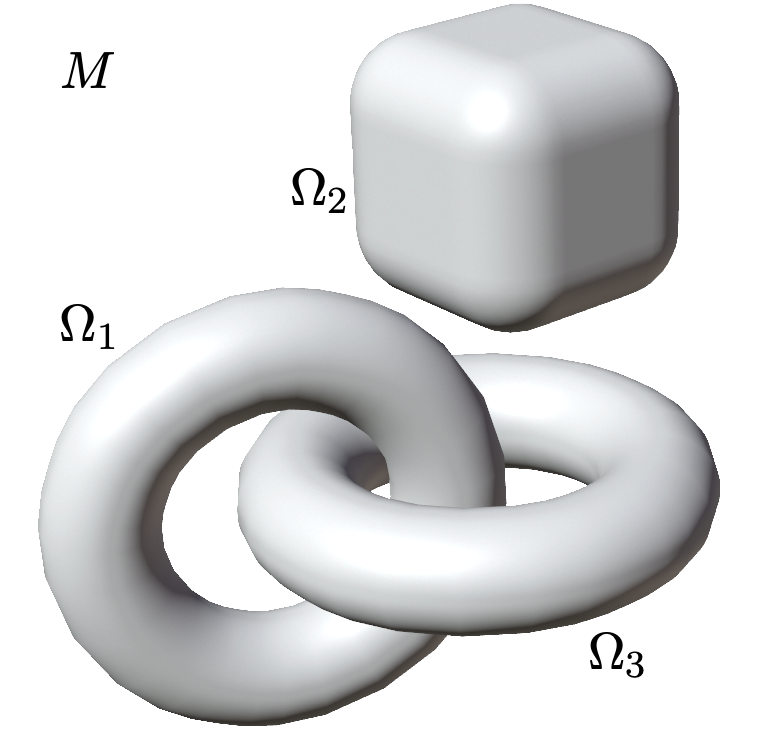
Let $\Omega$ be a bounded open subset of $\mathbb{R}^{d}$ with smooth boundary such that $M=\mathbb{R}^{d}\setminus\overline{\Omega}$ is connected. The domain $\Omega$ will be assumed to consist of $N$ many connected components $\Omega_{1},\ldots,\Omega_{N}$. The space $X=\mathbb{R}^{d}\setminus\partial\Omega$ therefore consists of the $N+1$-many connected components $\Omega_{1},\ldots,\Omega_{N},M$. We think of $\Omega$ as obstacles placed in $\mathbb{R}^{d}$. The open subset $M$ then corresponds to the exterior region of these obstacles. Similarly, we define $M_{i}=\mathbb{R}^{d}\setminus\overline{\Omega_{i}}$ and $X_{i}=\mathbb{R}^{d}\setminus\partial\Omega_{i}$.

Spectral and scattering theory describe the spectral resolution of these operators, which we now explain in more detail. A similar description as below is true in the more general black-box formalism in scattering theory as introduced by Sjöstrand and Zworski [37] and follows from the meromorphic continuation of the resolvent and its consequences. The description below follows [42] and we refer the reader to this article for the details of the spectral decomposition and properties of the scattering matrix.

The operators $\Delta_{\Omega}$ and $\Delta_{\Omega_{i}}$ have purely discrete spectrum, whereas $\Delta_{M}$ has purely absolutely continuous spectrum. The spectral resolution of $\Delta_{\Omega}$ is described by an orthonormal basis $(\phi_{j})$ of smooth eigenfunctions $\phi_{j}\in C^{\infty}(\overline{\Omega})$ with eigenvalues $\lambda_{j}^{2}$, where we assume

The eigenvalue counting function $\mathcal{N}_{\Omega}$ is defined by $\mathcal{N}_{\Omega}(\lambda)=\#\{\lambda_{j}<\lambda\}$ and satisfies a Weyl-law

for $\lambda\to+\infty$, where $C_{d}=(2\pi)^{-d}\omega_{d}$ and $\omega_{d}$ is the Euclidean volume of the unit ball in $\mathbb{R}^{d}$. The continuous spectral resolution of $\Delta_{M}$ is described by generalised eigenfunctions $E_{\lambda}(\Phi)\in C^{\infty}(\overline{M})$ indexed by $\lambda>0$ and $\Phi\in C^{\infty}({\mathbb{S}^{d-1}})$. The are uniquely determined by the following properties

1. (1)

   $(\Delta-\lambda^{2})E_{\lambda}(\Phi)=0$,

2. (2)

   $E_{\lambda}(\Phi)|_{\partial M}=0$

3. (3)

   The asymptotic expansion

   $$E_{\lambda}(\Phi)=\frac{\mathrm{e}^{-\mathrm{i}\lambda r}\mathrm{e}^{\frac{i\pi(d-1)}{4}}}{r^{\frac{d-1}{2}}}\Phi+\frac{\mathrm{e}^{\mathrm{i}\lambda r}\mathrm{e}^{-\frac{i\pi(d-1)}{4}}}{r^{\frac{d-1}{2}}}\Psi_{\lambda}+O\left(\frac{1}{r^{\frac{d+1}{2}}}\right),\quad\textrm{for}\,\,\,r\to\infty$$

   holds for some $\Psi_{\lambda}\in C^{\infty}({\mathbb{S}^{d-1}})$.

As a result $\Psi_{\lambda}$ is uniquely determined and implicitly defines a linear mapping

where $\tau:C^{\infty}({\mathbb{S}^{d-1}})\to C^{\infty}({\mathbb{S}^{d-1}})$ is the pull-back of the antipodal map. The map $\textbf{S}_{\lambda}:C^{\infty}({\mathbb{S}^{d-1}})\to C^{\infty}({\mathbb{S}^{d-1}})$ is called the scattering matrix, and $\textbf{A}_{\lambda}=\textbf{S}_{\lambda}-\mathrm{id}$ is called the scattering amplitude. The scattering matrix extends to a unitary operator $\textbf{S}_{\lambda}:L^{2}({\mathbb{S}^{d-1}})\to L^{2}({\mathbb{S}^{d-1}})$ for $\lambda>0$, and has the following properties depending on whether the dimension is even or odd.

• •

  In case $d$ is odd the scattering matrix $\textbf{S}_{\lambda}$ extends to a meromorphic function on $\mathbb{C}$ which is regular on the real line. It satisfies the functional relation $\textbf{S}_{\lambda}\tau\textbf{S}_{-\lambda}=\tau$ and is unitary in the sense that $(\textbf{S}_{\lambda})^{-1}=\textbf{S}_{\overline{\lambda}}^{*}$.

• •

  In case $d$ is even the scattering matrix $\textbf{S}_{\lambda}$ extends to a meromorphic function on the logarithmic cover of $\mathbb{C}\setminus\{0\}$. It is holomorphic in the upper half-plane and regular on $\mathbb{R}\setminus\{0\}$. We have a functional relation $\textbf{S}_{\lambda}\,\tau\,(2\,\mathrm{id}-\textbf{S}_{-\lambda})=\tau$, where $-\lambda$ is interpreted as $e^{\mathrm{i}\pi}\lambda$. Unitarity holds in the sense that $(\textbf{S}_{\lambda})^{-1}=\textbf{S}_{\overline{\lambda}}^{*}$.

It can be shown that $\textbf{A}_{\lambda}$ extends to a continuous family of trace-class operators on the real line and one has the following estimate on the trace norm

for all $|\lambda|<\frac{1}{2}$ in a fixed sector in the logarithmic cover of the complex plane, c.f. [42, Theorem 1.11] or [6, Lemma 2.5] in case $d\geq 3$.

If $f\in\mathcal{S}(\mathbb{R})$ is a Schwartz function with $f(\lambda)=f(-\lambda)$ we have that $f(\Delta_{X}^{\frac{1}{2}})-f(\Delta_{0}^{\frac{1}{2}})$ is a trace-class operator with trace equal to

for a function $\xi\in L^{1}_{\mathrm{loc}}(\mathbb{R})$ with $\xi(\lambda)=0$ if $\lambda<0$. The function is uniquely determined and called the spectral shift function. The Birman-Krein formula [3] states that for $\lambda>0$ one has

The relative trace and the relative trace formula were introduced in [19]. Suppose that $h$ is a polynomially bounded function and $\Delta_{X_{j}}$ as defined in Definition 1.1. Then each of the operators $h(\Delta_{X})$, $h(\Delta_{X_{j}})$, and $h(\Delta_{0})$ has $C^{\infty}_{0}(X)$ contained in its domain. We define

This operator has dense domain, containing $C^{\infty}_{0}(X)$. Whenever this operator is bounded (which is the only case we consider in this paper), we will denote its closure also by $\mathcal{R}_{h}$. If $h\in\mathcal{S}(\mathbb{R})$ is even then $\mathcal{R}_{h}$ is a trace-class operator and

where the relative spectral shift-function $\xi_{\mathrm{rel}}$ is for $\lambda>0$ given by

Here $\det(\textbf{S}_{j,\lambda})$ correspond to the scattering matrices when only obstacle $\Omega_{j}$ is present, and the other obstacles are removed. Note that the interior contributions cancel out. The main result of [19] is that $\mathcal{R}_{h}$ is trace-class for a much larger class of functions including $h(\lambda)=\lambda^{s}$ for $\operatorname{Re}(s)>0$. We briefly recall the result for a slightly less general class of functions that are sufficient for the purposes of this article. Define

for some $0<\theta\leq\pi$ and let $\mathcal{P}_{\theta}$ be the set of functions that are polynomially bounded, holomorphic in $\mathfrak{S}_{\theta}$, and satisfy the estimate $|g(z)|=O(|z|^{a})$ if $|z|<1$ for some $a>0$. If $f$ is a function such that $f(\lambda)=g(\lambda^{2})$ for some $g$ in $\mathcal{P}_{\theta}$ then $\mathcal{R}_{f}$ is trace-class and its trace can be computed by

for some universal function $\Xi$ that is independent of $f$. Here $\Gamma$ is the path in the complex plane consisting of the rays $(-\infty,0]\to\mathbb{C},t\mapsto-te^{\mathrm{i}\theta/2}$ and $[0,\infty)\to\mathbb{C},t\mapsto te^{\mathrm{i}(\pi-\frac{\theta}{2})}$. The function $\Xi$ is holomorphic in the upper half plane and satisfies on $\mathfrak{D}_{\epsilon}=\{\lambda\in\mathbb{C}\mid\operatorname{Im}(\lambda)>\epsilon|\lambda|\}$ the following bounds

for any $\delta^{\prime}$ with $0<\delta^{\prime}<\delta$ and $\epsilon>0$. In particular $\Xi$ is bounded in each sector near zero and is exponentially decaying at imaginary infinity. Here

denotes the minimum of the distances between distinct objects. The function $\Xi$ has a continuous boundary value on $\mathbb{R}$ and if $\lambda>0$ we have

Moreover, $\Xi(\lambda)$ can be expressed in terms of boundary layer operators as $\Xi(\lambda)=\log\det\left(Q_{\lambda}\tilde{Q}_{\lambda}^{-1}\right)$ (see [19, Theorem 1.7]). Here $Q_{\lambda}$ is the single layer operator for the Helmholtz equation on $\partial\Omega$ and $\tilde{Q}_{\lambda}$ is the direct sum of the single layer operators on the components $\partial\Omega_{j}$. This makes the function accessible both to numerical computation and to explicit estimates.

In this paper we link the asymptotic exponential decay rate of $\Xi$ with wave-trace invariants in the singularity expansion of the Fourier transform $\hat{\xi}_{\mathrm{rel}}$ of the relative spectral shift function $\xi_{\mathrm{rel}}$.

This is achieved by establishing a relationship between $\hat{\xi}_{\mathrm{rel}}$ and $\Xi$. Let $\theta=\chi_{[0,\infty)}$ be the Heaviside step function. Then, $\operatorname{Im}(\hat{\xi}_{\mathrm{rel}})$ vanishes near zero and $-4\pi\theta\cdot\operatorname{Im}(\hat{\xi}_{\mathrm{rel}})$ has a well defined Fourier-Laplace transform. We show in Section 4, that this Fourier-Laplace transform equals $\Xi(\lambda)$. This allows to translate properties of the wave-trace, a well studied object, to results for the function $\Xi(\lambda)$. In particular the singularity of the wave-trace at $t=2\delta$ determines the decay of $\Xi(\lambda)$ at imaginary infinity.

To demonstrate this we focus on the simplest case, when the obstacles are strictly convex near the points that have distance $\delta$ to other boundary components. In this case there exist only finitely many isolated non-degenerate bouncing ball orbits of length $2\delta$ between the obstacles and the corresponding leading wave trace-invariant at $t=2\delta$ can be computed explicitly. This leads to the following asymptotic behaviour for $\Xi$ valid uniformly in any sector of the form $\{\lambda\in\mathbb{C}\mid\operatorname{Im}(\lambda)>\alpha|\operatorname{Re}(\lambda)|\},\alpha>0$, namely

where the sum is over bouncing ball modes of length $2\delta$ and $P_{\gamma_{j}}$ is the associated Poincaré map. The precise formulation is in Theorem 3.7 and 4.1. This improves the a priori bounds (2) from [19] and allows for a geometric interpretation. Without convexity assumptions one has the bound

for any $0<\delta^{\prime}<\delta$ as a consequence of our finite propagation speed estimates uniformly in any sector of the form above.

Since the operator $(\Delta_{X}+1)^{-k}-(\Delta_{0}+1)^{-k}$ is a trace-class operator for all $k>(d-1)/2$ (see [4]), the classical Lifshits-Krein spectral shift function of the pair $(A,B)$ with $A=(\Delta_{X}+1)^{-k}$ and $B=(\Delta_{0}+1)^{-k}$ is the unique $L^{1}$-function $\xi_{AB}(\lambda)\in L^{1}(\mathbb{R})$ such that

for all $g\in C^{\infty}_{0}(\mathbb{R})$. The above identity is known to hold for $g$ in the Besov space $B^{1}_{\infty,1}(\mathbb{R})$, but is certainly true for $L^{1}$-functions whose derivative has $L^{1}$-Fourier transform. In fact, the most general class of admissible functions for $\xi_{AB}$ is the space of operator Lipschitz functions on $\mathbb{R}$ [30, 31]. Changing variables this shows that $f(\Delta_{X}^{\frac{1}{2}})-f(\Delta_{0}^{\frac{1}{2}})$ is trace-class with trace equal to

for all $f\in C^{1}([0,\infty))$ that satisfy

for some $k>(d-1)/2$. This is not the most general class of functions for which the above holds, but it will be sufficient for our purposes. From the above change of variables one obtains $\xi\in L^{1}(\mathbb{R},|\lambda|(1+\lambda^{2})^{-k-1}\mathrm{d}\lambda)$. By the bounds on $\|\textbf{A}_{\lambda}\|_{1}$ one in fact has $\xi\in L^{1}(\mathbb{R},(1+\lambda^{2})^{-k-1}\mathrm{d}\lambda)$ and $\xi$ is a piecewise continuous function vanishing at zero.

This implies that $\hat{\xi}$ is a tempered distribution. Since $\xi$ is supported in $[0,\infty)$ it is completely determined by its odd part $\xi_{\mathrm{o}}(\lambda)=\frac{1}{2}(\xi(\lambda)-\xi(-\lambda))$. Then

The distributional wave trace $w\in\mathcal{S}^{\prime}(\mathbb{R})$ is formally defined by

This formal expression needs to be interpreted in the sense of distributions, i.e. for each test function $\phi\in\mathcal{S}(\mathbb{R})$ one has

is a trace-class operator, and its trace is given by the pairing $(w,\phi)$. Here $\phi_{e}(t)=\frac{1}{2}(\phi(t)+\phi(-t))$ is the even part of $\phi$ and therefore $\hat{\phi}_{e}$ is the cosine transform of $\phi$. By the Birman-Krein formula we have that $(w,\phi)$ is equal to the pairing of $\mathrm{i}t\hat{\xi}_{\mathrm{o}}$ with $\phi$. As an immediate consequence of the definition of the spectral shift function one obtains

Now we would like to separate the absolutely continuous part $\xi_{ac}$ from the piecewise constant part $\xi_{p}$ of the spectral shift function. Let $\Pi_{M}:L^{2}(\mathbb{R}^{d})\to L^{2}(M)$ be the orthogonal projection. Then $\hat{\phi}_{e}(\Delta_{X}^{\frac{1}{2}})$ commutes with $\Pi_{M}$, but $\hat{\phi}_{e}(\Delta_{0}^{\frac{1}{2}})$ does not. However, we still have the decomposition

and

Here

and $\gamma_{d}$ is a homogeneous distribution given by

where $\underline{t}^{-d}$ is the homogeneous distribution defined in [18, Section 3.2] and $\boldsymbol{\delta}^{d-1}$ is the $d-1$-th distributional derivative of the delta distribution. Note that $\gamma_{d}(t)$ is the cosine Fourier transform of $(dC_{d})\lambda_{+}^{d-1}$ [34].

One can also consider the Cauchy evolution operator $U_{X}(t)$ which acts on the Hilbert space $L^{2}(X)\oplus L^{2}(X)$ and is given by

where $\Delta_{X}^{-\frac{1}{2}}\sin(t\Delta_{X}^{\frac{1}{2}})$ is defined by functional calculus with respect to the function $g(x)=x^{-\frac{1}{2}}\sin(x^{\frac{1}{2}}t)$, which is entire in $x$. This operator has finite propagation speed in the sense that its distributional kernel is supported away from the set $\{(x,y)\mid\mathrm{dist}(x,y)>t\}$. We similarly define $U_{X_{j}}$ and $U_{0}$. The corresponding distribution trace

then equals $2w(t)$.

The properties of $u$ (and hence $w$) have been subject to extensive investigation in various settings. This started with the work of Lax-Phillips [24, 25] in odd dimensions. Their method is also known as the Lax-Phillips semigroup construction [44, Chapter 9]. The trace of the Lax-Phillips semigroup can be expressed in terms of the scattering operator. By Lidskii’s theorem, the trace can also be written as a sum of the Fourier transform of the test function over the scattering frequencies (also known as resonances or scattering poles). It turns out that the trace of the Lax-Phillips semigroup is equal to the one of $u(t)$ [44, Chapter 9]. The trace-class property of $u$ on $(0,\infty)$ was shown by Bardos-Guillot-Ralston in [2] using the Birman-Krein formula (see also Melrose in [27] for potential scattering problems). By applying Ivrii’s work on the second Weyl coefficient [21], Melrose extended the trace formula to include $t=0$ for compact obstacles in [29]. There is a rich mathematical literature on estimates of the number of scattering poles in various settings based on trace-formulae, for instance, [28, 29, 32, 37, 38, 39].

The relation to geometry is facilitated by expressing the singular part of the wave-trace in terms of a sum of Lagrangian distributions with supports at the lengths of periodic trajectories. This is sometimes referred to as the Poisson summation formula for the wave trace. Thanks to the work of Chazarain [5], Colin de Verdière [7, 8], Duistermaat [10], Guillemin-Melrose [16], and Andersson-Melrose [1], the Poisson summation formula for the wave trace was derived for compact manifolds with or without boundary. We also refer to [35] for a very detailed treatment containing the case of manifolds with boundary. The standard assumptions for these results is strict geodesic concavity or convexity of the boundary. In the non-compact situation of obstacle scattering of finitely many strictly convex compact objects the Poisson summation formula is due to Bardos, Guillot, and Ralston [2]. We also refer to Petkov and Popov [33] for an overview and further results for non-trapping boundaries.

This theorem can be found in somewhat different language in [1, 16, 33] and is essentially Theorem 5 in [2]. It was first proved in a manifold setting by Melrose and Andersson [1] for compact manifolds. The theorem in the non-compact context can be reduced to the compact case using finite propagation speed arguments. Since such arguments are important in our approach we sketch it here for the sake of completeness.

In this section we assume throughout that number of connected components $N$ is at least two. We will study the singularities of $\hat{\xi}_{\mathrm{rel}}$ and the relative distributional wave-trace

Here $w_{j}(t)=\mathrm{Tr}\left(\cos(t\Delta_{X_{j}}^{\frac{1}{2}})-\cos(t\Delta_{0}^{\frac{1}{2}})\right)$ corresponds to $w(t)$ in the configuration where only the $j$-th obstacle $\Omega_{j}$ is present.

We start by preparing some observations about finite propagation speed which hold independent of convexity assumptions.

References

- [1] K. G. Andersson and R. B. Melrose. The Propagation of Singularities along Gliding Rays. Inventiones Math, 41:197–232, 1977.
- [2] C. Bardos, J.-C. Guillot, and J. Ralston. La relation de Poisson pour l’équation des ondes dans un ouvert non borné. Application à la théorie de la diffusion. Comm. Partial Differential Equations, 7(8):905–958, 1982.
- [3] M. Sh. Birman and M. G. Krein. On the theory of wave operators and scattering operators. Soviet Math. Dokl., 3: 740–744, 1962.
- [4] G. Carron. Déterminant relatif et la fonction xi. American Journal of Mathematics, 124(2): 307–352, 2002.
- [5] J. Chazarain. Formule de Poisson pour les variétés riemanniennes. Inventiones mathematicae, 24:65–82, 1974.
- [6] T. Christiansen. Weyl asymptotics for the Laplacian on asymptotically Euclidean spaces. American journal of mathematics, pages 1–22, 1999.
- [7] Y. Colin de Verdière. Spectre du Laplacien et longueurs des géodésiques périodiques. I. Compositio Mathematica, 27(1):83–106, 1973.
- [8] Y. Colin de Verdière. Spectre du Laplacien et longueurs des géodésiques périodiques. II. Compositio Mathematica, 27(2):159–184, 1973.
- [9] J. J. Duistermaat. On the Morse Index in Variational Calculus. Advances in Mathematics, 21:173–195, 1976.
- [10] J. J. Duistermaat and V. W. Guillemin. The spectrum of positive elliptic operators and periodic bicharacteristics. Inventiones mathematicae, 29:39–79, 1975.
- [11] J. J. Duistermaat and L. Hörmander. Fourier integral operators II. Acta Math., 128:184–269, 1972.
- [12] T. Emig and R.L. Jaffe. Casimir forces between arbitrary compact objects. Journal of Physics A: Mathematical and Theoretical, 41(16):164001, 2008.
- [13] Y. Fang and A. Strohmaier. A mathematical analysis of Casimir interactions I: The scalar field. https://arxiv.org/pdf/2104.09763, 2021.
- [14] Y. Fang and A. Strohmaier. A mathematical analysis of Casimir interactions II, The electromagnetic field. In preparation.
- [15] M. Ghomi. Shortest periodic billiard trajectories in convex bodies. Geom. funct. anal., 14: 295–302, 2004.
- [16] V. Guillemin and R. B. Melrose. The Poisson Summation Formula for Manifolds with Boundary. Adv. in Math., 32:204–232, 1979.
- [17] M. C. Gutzwiller. Periodic Orbits and Classical Quantization Conditions. J. Math. Phys., 12:343, 1971.
- [18] L. Hörmander. The analysis of linear partial differential operators I-IV. Springer-Verlag, Berlin, second edition, 2003.
- [19] F. Hanisch, A. Strohmaier and A. Waters. A relative trace formula for obstacle scattering. https://arxiv.org/pdf/2002.07291, 2020.
- [20] H. Hezari and S. Zelditch. Inverse Spectral Problem for Analytic -Symmetric Domains in . Annals of Mathematics, 170(1): 205–269, 2009.
- [21] V. Ya. Ivrii. Second term of the spectral asymptotic expansion of the Laplace–Beltrami operator on manifolds with boundary. Funktsional. Anal. i Prilozhen., 14(2):25–34, 1980.
- [22] O. Kenneth and I. Klich. Casimir forces in a T-operator approach. Phys. Rev. B, 78:014103, 2008.
- [23] V. V. Kozlov and D. V. Treshchev, translated by J. R. Schulenberger Billiards: A Genetic Introduction to the Dynamics of Systems with Impacts. Translations of Mathematical Monographs, 89, 1991.
- [24] P. Lax and R. Phillips, Scattering theory. Academic Press, New York, 1967.
- [25] P. Lax and R. Phillips, The time delay operator and a related trace formula, in “Topics in Functional Analysis”. Academic Press, New York, 1978.
- [26] R. B. Melrose. Microlocal parametrices for diffractive boundary value problems. Duke Math. J., 42(4):605–635, 1975.
- [27] R. B. Melrose. Scattering theory and the trace of the wave group. Comm. Partial Differential Equations, 45:29–40, 1982.
- [28] R. B. Melrose. Polynomial Bound on the Number of Scattering Poles. J. Funct. Anal., 53:287–303, 1983.
- [29] R. B. Melrose. Weyl asymptotics for the phase in obstacle scattering. Comm. Partial Differential Equations, 13(11):1431–1439, 1988.
- [30] V. V. Peller. The Lifshitz-Krein trace formula and operator Lipschitz functions. Proc. Amer. Math. Soc., 144:5207–5215 , 2016.
- [31] V. V. Peller. Operator Lipschitz functions (English translation). https://arxiv.org/abs/1611.01593, 2016.
- [32] V. Petkov Lower bounds on the number of scattering poles for several strictly convex obstacles. Asymptot. Anal., 30(1):81–91, 2002.
- [33] V. Petkov and G. Popov. Asymptotic behaviour of the scattering phase for non-trapping obstacles. Annales de l’institut Fourier, 32(3):111–149, 1982.
- [34] Y. Safarov. Fourier Tauberian theorems and applications. J. Funct. Anal., 185(1):111–128, 2001.
- [35] Y. Safarov and D. Vassiliev. The asymptotic distribution of eigenvalues of partial differential operators. American Mathematical Soc., 155, 1997.
- [36] Ya. G. Sinai. Dynamical Systems with Elastic Reflections. Russian Math.Surveys, 25(2):137–189, 1970.
- [37] J. Sjöstrand and M. Zworski. Complex scaling and the distribution of scattering poles. J. Amer. Math. Soc., 4(4):729–769, 1991.
- [38] J. Sjöstrand and M. Zworski. Lower bounds on the number of scattering poles. Comm. Partial Differential Equations, 18(5–6):847–857, 1993.
- [39] J. Sjöstrand and M. Zworski. Lower bounds on the number of scattering poles, II. J. Funct. Anal., 123(2):336–357, 1994.
- [40] J. Sjöstrand. A trace formula and review of some estimates for resonances, in Microlocal Analysis and Spectral Theory. NATO Adv. Sci. Inst. Ser. C Math. Phys. Sci., 490:377–437, 1997.
- [41] A. Strohmaier The classical and quantum photon field for non-compact manifolds with boundary and in possibly inhomogeneous media. arXiv:2011.12601
- [42] A. Strohmaier and A. Waters. Geometric and obstacle scattering at low energy. Communications in Partial Differential Equations., 45.11, 1451–1511.
- [43] A. Strohmaier and A. Waters. The Birman-Krein formula for differential forms and electromagnetic scattering. https://arxiv.org/pdf/2104.13589, 2021.
- [44] M. E. Taylor. Partial differential equations II. Qualitative studies of linear equations, volume 116 of Applied Mathematical Sciences. Springer, New York, second edition, 2011.
- [45] A. Wirzba, The Casimir effect as scattering problem. J. Phys. A: Math. Theor., 164003, 2008.
- [46] S. Zelditch. Inverse Spectral Problem for Analytic Domains I: Balian-Bloch Trace Formula. Communications in Mathematical Physics, 248: 357–407, 2004.
- [47] S. Zelditch. Inverse Spectral Problem for Analytic Domains, II: -Symmetric Domains. Annals of Mathematics, 170(1): 205–269, 2009.