Quantum state discrimination for supervised classification
Abstract.
In this paper we investigate the connection between quantum information theory and machine learning. In particular, we show how quantum state discrimination can represent a useful tool to address the standard classification problem in machine learning. Previous studies have shown that the optimal quantum measurement theory developed in the context of quantum information theory and quantum communication can inspire a new binary classification algorithm that can achieve higher inference accuracy for various datasets. Here we propose a model for arbitrary multiclass classification inspired by quantum state discrimination, which is enabled by encoding the data in the space of linear operators on a Hilbert space. While our algorithm is quantum-inspired, it can be implemented on classical hardware, thereby permitting immediate applications.
1. Introduction
Quantum theory constitutes a new paradigm for information processing and provides unconventional ways to address computational problems. Advances in quantum computing have led to the development of algorithms that utilize quantum hardware to solve certain problems dramatically faster than any foreseeable classical hardware [1, 2, 3, 4]. A commercially relevant family of problems for which the application of quantum algorithm promises certain computational benefits are found in the domain of machine learning. This gave birth to the new discipline known as quantum machine learning (QML). Several quantum machine learning algorithms have been proposed with clear quantum advantages [5, 6, 7, 8, 9, 10]. However, the practical application of these algorithms are limited by the development of quantum hardware, which remains a long-term prospect.
Advances in quantum computing have led to another intriguing stream of research which aims to develop new classical algorithms inspired by quantum information processing to outperform existing methods, namely quantum-inspired classical algorithms [11, 12, 13]. The implications of this approach is significant not only for the domain of computational complexity theory, but also for practical applications. The complexity of implementing quantum machine learning algorithms on a quantum hardware and the emergence of quantum-inspired classical algorithms motivate the development of quantum-inspired machine learning (QIML) [14]. In principle, QIML deals only with “mathematically quantum objects”: objects that are formally represented by different elements of the quantum formalism (such as density operators, also known as density matrices), but are not necessarily connected to actual quantum systems. Thus, the information stored in those objects can be formally managed by a classical computer. Recent findings show that the well-developed field of quantum state discrimination in quantum information theory and quantum communication can inspire new pattern recognition algorithms that can improve the binary classification accuracy of existing methods [15, 16, 17, 18].
In this work, we first explain the connection between quantum state discrimination and the quantum-inspired binary classification cited above, and then propose a quantum-inspired supervised machine learning algorithm for arbitrary multiclass classification. Our algorithm is based on using the mathematical framework of quantum mechanics to represent data and a quantum state discrimination technique known as Pretty Good measurement. We show the theoretical derivation of this measurement strategy in the context of multiclass classification tasks in machine learning. We also show the classification accuracy of this quantum-inspired multiclass classifier can be improved by increasing the number of copies of the quantum object that encodes the data, at the cost of increasing the computational time. Since our approach does not require quantum hardware, it can be immediately implemented on existing classical hardware.
The paper is organized as follows. In Section 1, we provide a brief introduction regarding the general setting for supervised classification. In Section 2, the idea of quantum-inspired classifiers are described in detail. Section 3 is devoted to show the connection between quantum state discrimination and supervised classification; in particular, we provide some significant comments about quantum-inspired binary classification and then we introduce a more general quantum-inspired multiclass classification. Some final comments close the paper.
2. General setting for supervised classification
Supervised classification is one of the most important branches in machine learning [19]. It essentially consists of designing algorithms which learns by example in order to classify objects. The term supervised refers to the intuitive idea that the entire process is supervised by an “expert” who first builds up a preliminary set of correctly classified objects and then, on the basis of this dataset (called the training dataset), an algorithm is applied which would then allow one to classify new “unseen” objects (or objects from the training dataset) as accurately as possible.
Objects are described by a sequence number of features considered to be sufficiently relevant to characterize the objects in the classification framework. More formally, any object is associated to a vector (called object-vector or feature-vector) of a -dimensional Hilbert space 11 1 Unlike the standard presentations in machine learning, we do not exclude features which may be represented as complex numbers. The feature-vector can be the raw data itself, or can be obtained via feature mapping from a lower dimensional space.. We define a pattern as a pair
where is a feature-vector and is the class label which denotes the class with which the object is supposed to belong to. For simplicity, we identify the set of all class labels with a finite sequence of natural numbers that are in one-to-one correspondence with the classes which the objects belong to. Thus, a training dataset can be represented as a set
where , . Given any class label , we can define the set of all object-vectors whose associated class label is :
| (2.1) |
The cardinality of is denoted by . Clearly, .
The task of supervised classification is to infer a function from the training dataset using an algorithm (a classifier) which would classify objects into one of the classes that the object is supposed to belong to, thus assigning a class label to an object-vector as accurately as possible.
Formally, a classifier can be defined as a map
There are several well known classification approaches in which different classifiers employ to classify objects, such as distance-based or probability-based classification approaches. In this paper, we present the following probability-based classification approach. Given a training dataset
one defines a map that associates to any feature-vector a sequence of -numbers belonging to the unit real-interval
The -component of will be denoted by .
The meaning of depends on the function . For example, if is assumed to be a probability-vector (i.e. ), the value can be interpreted as the probability that the object (with associated feature-vector ) belongs to the class labelled by .
The classifier determined by (or simply, the -classifier) is the map
that assigns to any feature-vector the class label that is associated to the greatest value of , with . In other words,
Since it may happen that returns more than one class label when there are matching values, we pose by convention
| (2.2) |
A classifier is called probabilistic iff In other words, a classifier is probabilistic iff the sequence is a probability-vector for any .
3. Quantum classifiers
Since object-vectors are defined in the Hilbert space, it is natural to treat it as a quantum state and apply mathematical techniques from quantum information theory. The underlying idea of this work is to encode object-vectors as density operators, and construct a classifier based on the quantum measurement technique developed in the realm of quantum information theory to optimally discriminate quantum states. In the following, we describe our encoding strategy for representing the set of object-vectors as density operators.
3.1. Basic framework
Given a training dataset, the construction of a quantum classifier is based on three fundamental steps: i) obtain a quantum feature map (or encoding) to encode the object-vectors of the training dataset into quantum objects (see Appendix A); ii) find an appropriate function that determines the quantum classifier; iii) apply the quantum classifier to the quantum encoded object-vectors to obtain class labels for the original (classical) objects.
Let us consider a training dataset . A quantum feature map (or encoding) is a map that associates to any object-vector of a pure quantum state (called object quantum-state) of a Hilbert space , whose dimension depends on the number of features. An example of quantum encoding is described in Appendix A (also see [17]). Without loss of generality, we use the density operator denoted by rather than the state vector formalism to describe quantum states. Note that the density operator formalism follows naturally when we describe multiple object-vectors as mixed states in the following. Given a quantum encoding , a quantum pattern is any pair
A quantum training dataset is defined as the set of all quantum patterns
Given any class label , we can also define the set as the set of all object quantum-states that are associated to the set of all -objects vectors:
| (3.1) |
Definition 3.1.
Let be a class label. The quantum centroid associated to denoted by is the uniformly weighted convex combination of all -object quantum-states
where is the cardinality of (which is equivalent to , the cardinality of ).
Thus, the class labels are in one-to-one correspondence with the set for all quantum centroids.
Remark 3.1.
Let us consider the classical centroid and let the quantum encoding of the classical centroid . In general we can see that . In other words, the quantum centroid defined in Def. 3.1 does not correspond to the quantum encoding of the classical centroid.
Remark 3.2.
Let us consider a -dimensional vector . In the classical case, the translation of the object-vector results in the translation of the classical centroid as . However, the quantum centroid related to the object quantum-states turns out to be non-translational invariant. This characteristic is shown to be beneficial for classification tasks [16, 20].
Let be a training dataset with class labels .
Let be the set of bounded and positive semidefinite operators acting on . A quantum classifier is a classifier , where the function is determined by a measurement (see [21], Def. 2.34).
Recall that a measurement is defined as a map from a finite non-empty set representing a set of possible outcomes of a physical quantity into , such that . In the case of von Neumann measurements, every is a projection.
We can now define formally the notion of a quantum classifier.
Definition 3.2.
A quantum classifier is a classifier (see Eq.(2.2)) for which the map satisfies the following condition. There exists a measurement such that
where tr is the trace of a matrix.
By definition of measurement,
. Consequently, a quantum classifier is always probabilistic.
3.2. Encoding in a larger Hilbert space
An interesting question is whether classification accuracy can be improved by increasing the dimension of the state space of density matrices that represents feature-vectors. Since mapping a raw dataset in a low-dimensional feature space to a higher-dimensional feature space is a standard technique in the kernel method, such question arises naturally. Although the computation in the larger feature space increases the run time, the accurate prediction has more value in certain machine learning applications, such as those specialized in medical diagnosis. In particular, we consider encoding object-vectors as the tensor product of copies of object quantum-states , i.e. . In this case, we generalize the set defined in Eq. (3.1) as
Similarly, the copies-centroid can be defined as
| (3.2) |
From the definition above, we should keep in mind that, in general, . With the construction above, the -generalization of a quantum classifier introduced in Def. 3.2 can be defined by a function and by a measurement . As we will show, this procedure turns out to be advantageous in improving classification accuracy.
4. Classification inspired by quantum state discrimination
Since feature-vectors are defined as quantum states, we can conceptualize the machine learning task as finding an optimal quantum measurement for the feature-vectors, with respect to the quantum centroids. This permits the development of the new classification procedure inspired by quantum state discrimination [22, 23, 24], which is a well-established field in the theory of quantum information [21]. To make the connection more apparent, we briefly review quantum state discrimination as follows.
4.1. Quantum state discrimination
The task of discriminating quantum states is a fundamental problem in quantum information theory, with deep implications in quantum cryptography and quantum error correction [25]. The problem of quantum state discrimination can be summarized as follows. Let us suppose that Alice wishes to send a message to Bob by using a quantum channel. To do this, Alice selects a state with an a priori probability from a given set of possible states in the Hilbert space . We indicate the set of these possible states with their respective a priori probabilities as follows
where is a probability-vector (a sequence of positive real numbers such that ).
Bob knows a priori both the set of possible states and the associated probabilities. His task is to determine, by means of a suitably chosen measurement, the state he receives from Alice, and hence, the intended message. But the problem of finding an optimal strategy for discrimination among arbitrary states, has no known solution in the general case. While optimal solutions can be found for some particular cases (as, for example, when contains only mutually orthogonal states), in general, errors will necessarily occur in the discrimination process (see for example [24]). This means that, in general, there exists no measurement such that when , . Thus, once Alice sends the -th state to Bob, he can either conclude (erroneously) that he was given the state or, conversely, he can conclude (correctly) that he was given the state (successful discrimination). The average probability for Bob to perform a successful discrimination by means of a given measurement is given by
| (4.1) |
In order to minimize the error probability in the discrimination problem, it is necessary to find an optimal measurement which maximizes Eq. (4.1). Or equivalently, that minimizes the discrimination error probability . One can prove (see [21]) that, for any ensemble , there exists an optimal measurement (shortened to ), such that
4.2. Helstrom measurement and binary classification
In 1969, Helstrom reported an exact analytical description for the optimal measurement for ensembles of two quantum states [22]. Let
be an ensemble of two quantum states with a priori probabilities and . Let us define the Helstrom observable as
| (4.2) |
Let and be the sets of all the eigenvectors determined by the positive and negative eigenvalues of , respectively. Let and , where indicates the projection associated to the eigenspace determined by the eigenvalue . Intuitively, and represent the property of the measurement to correctly identify a state as being in state or , respectively. The set determines a von Neumann measurement, given that (see Appendix B). Helstrom proved that this measurement is optimal and the probability to successfully discriminate correctly between the two states has an upper bound [22] – called Helstrom bound – given by
| (4.3) |
It turns out (see [21]) that
where is the trace distance induced by the trace norm ,
In the case when , we will simply write instead of . satisfies the following properties (see [21]):
- i)
;
- ii)
iff ;
- iii)
iff is orthogonal to , where is the subspace spanned by the image of .
Under Helstrom’s formalism, let us now consider the particular case for binary classification, where . After quantum encoding, we obtain the quantum training datasets and , defined in accordance with Eq. (3.1), and and as the respective quantum centroids obtained from Def. 3.1. In this way, it is possible to define the Helstrom observable (as in Eq. (4.2)) for the two quantum centroids and , where and are the a priori probabilities given by and , respectively. In this case, the quantum classifier introduced in Def. 3.2 for an arbitrary new “unseen” object quantum-state (or from the quantum training dataset) is given by
An experiment is shown in [15], where the Helstrom Quantum Centroid (HQC) classifier is applied to fourteen different datasets and compared with eleven different standard classifiers, with the HQC classifier exhibiting a high level of accuracy performance when compared to these standard classifiers. In that paper, the application of the quantum state discrimination procedure to the problem of classification tasks gave rise to the following notable observation: the higher the probability of successfully discriminating between quantum centroids, the better the accuracy performance of the quantum classifier. In other words, for the binary classification case, if one manages to increase the Helstrom bound (considered as a measure of distinguishability between the two quantum centroids), then one would expect the accuracy of the quantum classifier to be higher. The experiment given in [15] provides an empirical evidence of this intuition. Also as shown in Fig. 1, for the given fourteen datasets that were investigated, we obtained a Pearson coefficient of which indicates a strong positive (linear) relationship between the Helstrom bound and balanced accuracy score.

4.2.1. Advantages of encoding in a larger Hilbert space
As discussed at the end of Section 3, it is possible to perform the tensor product of copies of each object quantum-state. This allows us to define the new quantum centroids and . Consequently, the respective Helstrom measurement is given by . In this way, the quantum classifier takes the form
The empirical results obtained in [15] strongly suggest that taking tensor products of artificial copies of the object quantum-states turns out to be beneficial for classification tasks. As a theoretical support to this claim, in this paper, we prove the following.
Theorem 4.1.
For any ,
Proof.
See Appendix II. ∎
According to Theorem 4.1, increasing the number of copies of the object quantum-states (and consequently, increasing the number of factors in the tensor product) gives a higher Helstrom bound (which means a higher success probability for discriminating the two quantum centroids). As a result, the accuracy performance of the quantum classifier increases. As an example, by applying the HQC classifier to six different datasets (in the experiment as detailed in [15]), we show in Fig. 2 how the application of this procedure improves the accuracy performance measured by three different statistical scores (balanced accuracy, f1-score and k-Cohen).

Many questions remain open, and an extensive investigation into the relation between the Helstrom bound and the statistical scores in machine learning problems is still ongoing. The results obtained so far motivates further research into this.
It is also relevant to note that, even if increasing the number of copies in the tensor product, in principle, produces an improvement to the accuracy performance of the quantum classifier, at the same time it also produces an additional computational cost (i.e. run time of the algorithm). Hence, depending on the size of the dataset and on the machine being used, the maximum number of tensor copies should be chosen by a user based on practical considerations. This leads to another interesting future work that aims to utilize quantum hardware to speedup the classification protocol.
4.3. Pretty Good measurement and multiclass classification
A common strategy to perform multiclass classification is based on combinatorial compositions of binary classifications (i.e. One-vs-One or One-vs-Rest strategies). One disadvantage with these strategies is that if a dataset contains a large number of classes, it would increase the computational time of the algorithm. In the following, we show how quantum state classification suggests an alternative method which allows us to avoid this combinatorial complexity for multiclass classification.
Given an ensemble of possible states with their respective a priori probabilities
| (4.4) |
it may be difficult to find an analytical description for the exact optimal measurement associated to . One possible solution is to search for a sub-optimal measurement that can be expressed in an analytical form. This is known as the so-called Pretty Good measurement [21], which we will introduce in the following.
Let us define the average state of as
For any , let us define the following operator
where is the pseudoinverse (or Moore-Penrose inverse) of . The operator is well defined. Indeed, by Theorem C.1 (iv) (see Appendix C), is positive since is positive and consequently, the square root of exists and is unique. Since is positive semidefinite and it is enclosed on the left and on the right by a self-adjoint operator , we conclude is also positive semidefinite (see [26], p.431). By Theorem C.1 (vi) (see Appendix C), we have . Consequently, by Theorem 6.6.4 (see [27], p.223), commutes with . As a result, we have
| (4.5) |
by Theorem C.1 (vi), where is the projection onto the subspace spanned by the image of .
From Theorem C.1 (vi), is a projection. Since any is positve semidefinite, we have that is bounded by the identity operator and therefore it is an effect operator: . However, the set does not determine a measurement since in general . The set can easily be transformed into a set of effects that finally induce a measurement.
For any with , let us define the following operators
| (4.6) |
where is the projection associated to the subspace spanned by the kernel of . It turns out that the map
is a measurement since, as we have seen above, and consequently
| (4.7) | ||||
We have now induced a measurement where . Since is invertible iff , we can conclude, from Eqs. (4.5) and (4.7), that iff is invertible.
Let us now turn to the general problem of multiclass classification. We will follow a similar formalism to that of the Helstrom observable (for the binary classification case), but using a classifier based on the Pretty Good measurement formalism. After the quantum encoding procedure, we consider the quantum training datasets as defined in Eq. (3.1) and the respective quantum centroids as defined in Def. 3.1. Hence, it is possible to consider the ensamble as defined in Eq. (4.4) where (for any ). In this way, induces a set of operators as defined in Eq. (4.6). In this case, the multiclass quantum classifier introduced in Def. 3.2 for an arbitrary new “unseen” object quantum-state (or from the quantum training dataset) is given by
| (4.8) |
Notice that if , we can replace by in the above equation.
We can also generalize this framework by taking the tensor product of copies of states. Thus, the definition of the multiclass quantum classifier introduced in Eq. (4.8), can naturally be extended as
As in the Helstrom measurement case, it is possible to define a bound for the Pretty Good measurement as follows
It is currently not known whether it is possible to obtain a general result regarding the relation between the value of the PGM bound and the number of tensor products (as in Theorem 4.1) for the Pretty Good measurement classifier. We present an initial insight and empirical evidence on this, suggesting an analogous result, in Appendix D.
5. Conclusion
In this work we have established a connection between the problems of quantum state discrimination and classification tasks in the machine learning context. Specifically, we assert that the former can provide relevant benefits to the latter. The proposed strategy is based on the following steps. First we obtain a quantum feature map (or encoding) of real feature-vectors to pure quantum states, then to each class we associate a quantum centroid as a mixed quantum state. In other words, the feature space is defined by the space of linear operators on a Hilbert space. Next we develop a quantum version of the supervised classification task that has the general property that the performance of the classification process increases with the capability of distinguishing among the quantum centroids. We have presented theoretical and empirical evidences to support this. Finally, we show that in the quantum framework, making duplicate copies of the initial data turns out to be beneficial for the classification process. This idea is similar to increasing the dimension of the feature space that is encountered in the kernel trick. This strategy, previously provided only for binary classification, is hereby introduced in the general setting for multiclass classification developed using the Pretty Good measurement formalism.
Appendix A Quantum feature maps (encodings)
There are, or course, infinitely many ways to map an object-vector into a density matrix. Different encodings have been already considered in previous works [17]. Here, as an instance, we focus on the following encoding procedure. For each , let
Next, we give the following.
Definition A.1.
The amplitude encoding is the map
Note that is a pure state in . We say that is the object quantum-state associated to object-vector .
Appendix B Helstrom bound and tensor copies
In this Appendix we give the proof of Theorem 4.1:
For any ,
Proof.
Since the Helstrom bound of two density operators and is given by – where is the trace distance induced by the trace norm – in order to prove Theorem 4.1, it suffices to show that
Let us consider the Hilbert space , where and . Let be the partial trace of the first component of , i.e., .
Using linearity of the partial trace operator
| (B.1) |
The above list of equations can be physically interpreted as follows: if one has a product state of components, tracing out the first system will not alter the rest of the states. Similarly,
| (B.2) |
The trace distance satisfies a contractivity property under the action of complete trace preserving of positive maps (i.e., trace preserving quantum operators, see [30]). Since is a trace-preserving quantum operation, we have that
| (B.3) |
Thus, by Eqs. (B.1), (B.2) and (B.3) we can conclude that
∎
Appendix C Mathematical properties of the pseudoinverse
Let be the finite complex Hilbert space of dimension . will denote the set of all positive semidefinite bounded linear operator of . The set of all projections of will be denoted by . Using we will denote the set of all effects of , i.e. the set of all positive operator in that are bounded by the identity operator . Thus, an effect is a an operator of such that .
Definition C.1.
Let be a linear operator of . The pseudoinverse (or Moore-Penrose inverse) of is an operator of such that the following conditions are satisfied:
- i)
;
- ii)
;
- iii)
, where † is the adjoint operation;
- iv)
.
One can prove that the pseudoinverse of any operator exists and is unique. The pseudoinverse of an operator will be denoted by . It turns out that if is invertible, then the inverse of (i.e. ) coincides with .
Theorem C.1.
Let be a linear operator of . The following properties hold:
- i)
is invertible iff ;
- ii)
;
- iii)
;
- iv)
if , then ;
- v)
and are projections;
- vi)
if , then , where is the projection that projects onto the image of .
Appendix D An example of the PGM bound and tensor copies.
Theorem D.1.
Let us consider the special quantum datasets and (representing 2 classes) where and are diagonal matrices, i.e. and , with .
Also lets consider the datasets and .
Let us calculate the quantum centroids for the sets and : and and, analogously, for the sets and : and
Let and , the Pretty Good measurement bound built over and and the Pretty Good measurement bound built over and , respectively.
We show that for any initial sets and .
Proof.
Following the standard procedure of the formalism, we first calculate the average state
Then, we calculate:
and
where represents the pseudoinverse function. Let us notice that, given the fact that has a diagonal form, then the pseudoinverse coincides with the inverse and consequently .
Now let us calculate . By a straightforward calculation, it follows that:
Following the same strategy, it is possible to define , , and . It can be easily shown that the difference between and can be written as: where
It trivially follows that , , and are non-negative and .
It can be seen that for and for these values (which provides the minimum difference) . Hence our claim holds.
∎
In an analogous way, it is possible to define , and so on. We empirically study the effect of increasing the number of tensor copies (i.e. increasing the dimension of the feature space) on the PGM bound via numerical simulations based on random 2-feature vectors. The simulation results are shown in Fig. 3.
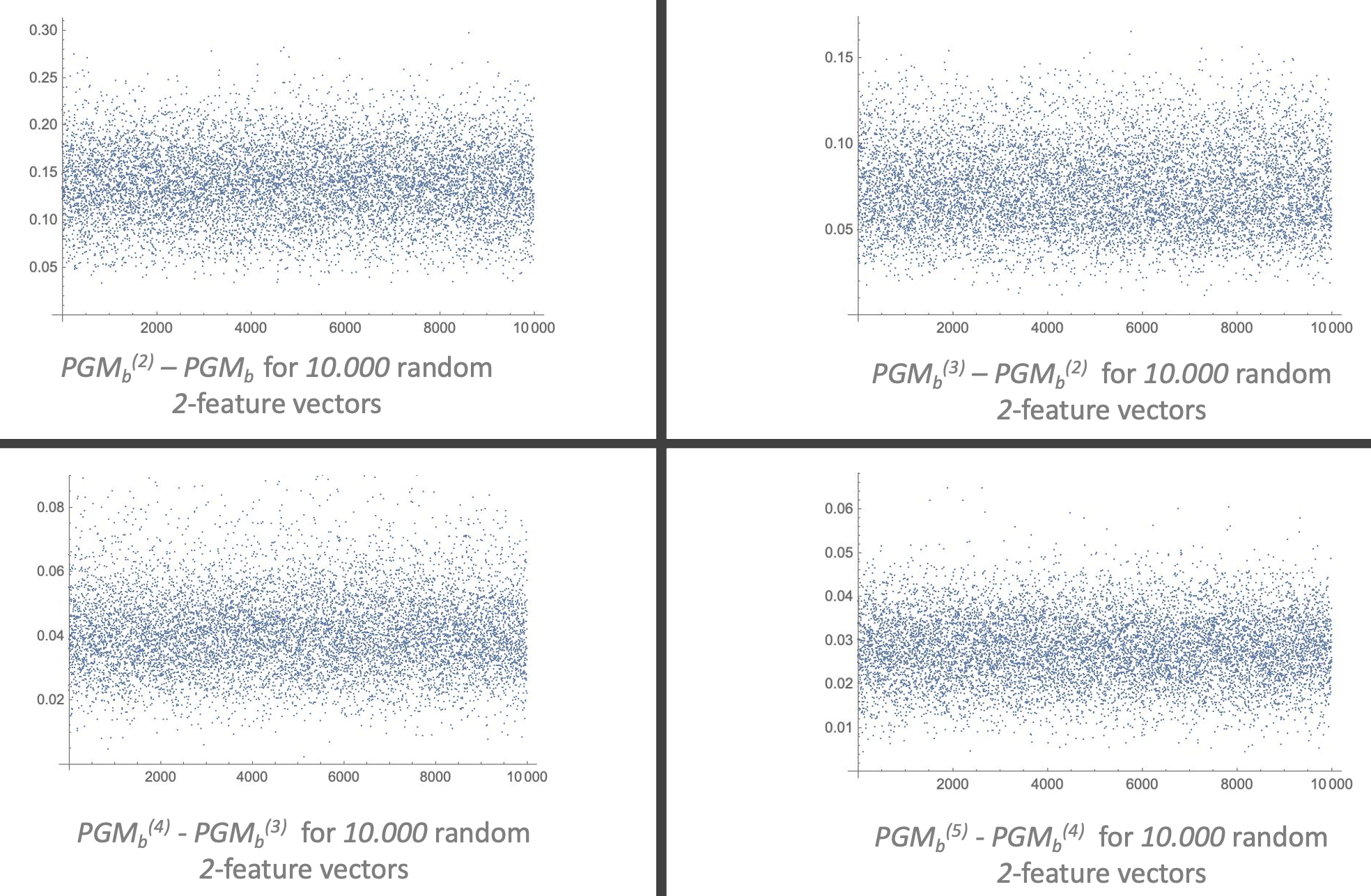
These results show how . A formal and general proof of this observation remains a future work.
Acknowledgments
D.K.P. gratefully acknowledges support from the National Research Foundation of Korea (No. 2019R1I1A1A01050161), and Quantum Computing Development Program (No. 2019M3E4A1080227). R.G gratefully acknowledges support from the R.G. is grateful to the RAS (Regione Autonoma della Sardegna) (project code: RASSR40341, A Semantic Extension of Quantum Computationsl Logic). G.S. is grateful to Fondazione di Sardegna (project code: F71I17000330002) and to the Prin project “Logic and Cognition. Theory, experiments, and applications”.
References
- [1] Seth Lloyd. Universal quantum simulators. Science, 273(5278):1073–1078, 1996.
- [2] Christof Zalka. Simulating quantum systems on a quantum computer. Proceedings of the Royal Society of London. Series A: Mathematical, Physical and Engineering Sciences, 454(1969):313–322, 1998.
- [3] Peter W Shor. Polynomial-time algorithms for prime factorization and discrete logarithms on a quantum computer. SIAM review, 41(2):303–332, 1999.
- [4] Aram W. Harrow, Avinatan Hassidim, and Seth Lloyd. Quantum algorithm for linear systems of equations. Phys. Rev. Lett., 103:150502, Oct 2009.
- [5] Patrick Rebentrost, Masoud Mohseni, and Seth Lloyd. Quantum support vector machine for big data classification. Phys. Rev. Lett., 113:130503, Sep 2014.
- [6] Seth Lloyd, Masoud Mohseni, and Patrick Rebentrost. Quantum principal component analysis. Nature Physics, 10(9):631–633, 2014.
- [7] Maria Schuld, Ilya Sinayskiy, and Francesco Petruccione. Prediction by linear regression on a quantum computer. Phys. Rev. A, 94:022342, Aug 2016.
- [8] Nana Liu and Patrick Rebentrost. Quantum machine learning for quantum anomaly detection. Phys. Rev. A, 97:042315, Apr 2018.
- [9] Carsten Blank, Daniel K. Park, June-Koo Kevin Rhee, and Francesco Petruccione. Quantum classifier with tailored quantum kernel. npj Quantum Information, 6(1):41, May 2020.
- [10] Daniel K. Park, Carsten Blank, and Francesco Petruccione. The theory of the quantum kernel-based binary classifier. Physics Letters A, 384(21):126422, 2020.
- [11] Ewin Tang. A quantum-inspired classical algorithm for recommendation systems. In Proceedings of the 51st Annual ACM SIGACT Symposium on Theory of Computing, STOC 2019, page 217–228, New York, NY, USA, 2019. Association for Computing Machinery.
- [12] Ewin Tang. Quantum-inspired classical algorithms for principal component analysis and supervised clustering, 2019. arXiv:1811.00414.
- [13] Juan Miguel Arrazola, Alain Delgado, Bhaskar Roy Bardhan, and Seth Lloyd. Quantum-inspired algorithms in practice. Quantum, 4:307, August 2020.
- [14] Federico Holik, Giuseppe Sergioli, Hector Freytes, and Angelo Plastino. Pattern recognition in non-kolmogorovian structures. Foundations of Science, 23(1):119–132, 2018.
- [15] Giuseppe Sergioli, Roberto Giuntini, and Hector Freytes. A new quantum approach to binary classification. PLOS ONE, 14(5):1–14, 05 2019.
- [16] Giuseppe Sergioli, Gustavo Martin Bosyk, Enrica Santucci, and Roberto Giuntini. A quantum-inspired version of the classification problem. International Journal of Theoretical Physics, 56(12):3880–3888, 2017.
- [17] Giuseppe Sergioli, Giorgio Russo, Enrica Santucci, Alessandro Stefano, Sebastiano Emanuele Torrisi, Stefano Palmucci, Carlo Vancheri, and Roberto Giuntini. Quantum-inspired minimum distance classification in a biomedical context. International Journal of Quantum Information, 16(08):1840011, 2018.
- [18] Giuseppe Sergioli, Carmelo Militello, Leonardo Rundo, Luigi Minafra, Filippo Torrisi, Giorgio Russo, Keng Loon Chow, and Roberto Giuntini. A quantum-inspired classifier for clonogenic assay evaluations. Scientific Reports, 11(1):2830, 2021.
- [19] Trevor Hastie, Robert Tibshirani, and Jerome Friedman. The Elements of Statistical Learning: Data Mining, Inference, and Prediction, Second Edition. Springer Series in Statistics. Springer New York, 2009.
- [20] Enrica Santucci and Giuseppe Sergioli. Classification problem in a quantum framework. In Andrei Khrennikov and Bourama Toni, editors, Quantum Foundations, Probability and Information, pages 215–228. Springer International Publishing, Cham, 2018.
- [21] John Watrous. The Theory of Quantum Information. Cambridge University Press, 2018.
- [22] Carl W. Helstrom. Quantum detection and estimation theory. Journal of Statistical Physics, 1(2):231–252, Jun 1969.
- [23] Stephen M. Barnett and Sarah Croke. Quantum state discrimination. Adv. Opt. Photon., 1(2):238–278, Apr 2009.
- [24] Joonwoo Bae and Leong-Chuan Kwek. Quantum state discrimination and its applications. Journal of Physics A: Mathematical and Theoretical, 48(8):083001, jan 2015.
- [25] Charles H. Bennett and Gilles Brassard. Quantum cryptography: Public key distribution and coin tossing. Theoretical Computer Science, 560:7–11, 2014. Theoretical Aspects of Quantum Cryptography, celebrating 30 years of BB84.
- [26] Roger A. Horn and Charles R. Johnson. Matrix Analysis. Cambridge University Press, 2 edition, 2012.
- [27] A. Friedman. Foundations of Modern Analysis. Dover Books on Mathematics Series. Dover, 1982.
- [28] Paul Hausladen and William K. Wootters. A pretty good measurement for distinguishing quantum states. Journal of Modern Optics, 41(12):2385–2390, 1994.
- [29] H. Barnum and E. Knill. Reversing quantum dynamics with near-optimal quantum and classical fidelity. Journal of Mathematical Physics, 43(5):2097–2106, 2002.
- [30] Mary Beth Ruskai. Beyond Strong Subadditivity? Improved Bounds on the Contraction of Generalized Relative Entropy, pages 350–366. World Scientific Publishing, 1994.