On cost design in applications of optimal control

Taouba Jouini Anders Rantzer Thanks: *This work has received funding from the European Research Council (ERC) under the European Union’s Horizon 2020 research and innovation program (grant agreement No: 834142) and the Swedish Research Council (grant 2019-0069). Thanks: The authors are with the Department of Automatic Control, LTH, Lund University, Lund, Sweden. E-mails: {taouba.jouini, anders.rantzer}@control.lth.se.

Abstract

A new approach to feedback control design based on optimal control is proposed. Instead of expensive computations of the value function for different penalties on the states and inputs, we use a control Lyapunov function that amounts to be a value function of an optimal control problem with suitable cost design and then study combinations of input and state penalty that are compatible with this value function. This drastically simplifies the role of the Hamilton-Jacobi-Bellman equation, since it is no longer a partial differential equation to be solved, but an algebraic relationship between different terms of the cost. The paper illustrates this idea in different examples, including $\mathcal{H}_{\infty}$ control and optimal control of coupled oscillators.

Index Terms:

Optimal control, Stability of nonlinear systems, Lyapunov methods

I Introduction

The objective in optimal control problems is to transfer the state of a dynamical system with minimum cost from one point to another. The advent of modern control theory, particularly the formulation of the famous Maximum Principle of Pontryagin [1] has had a considerable impact on the treatment of optimization theory. Dynamic programming gives necessary and sufficient conditions for optimality and optimal control laws in feedback form, which are very satisfactory but suffer from several drawbacks [2, 3]. First, analytic solutions can only be obtained in few cases (in particular linear quadratic problems). Second, the Hamilton-Jacobi-Bellman (HJB) partial differential equation (PDE) is in general very hard to solve numerically. The main problem is that the full state space must be discretized and a huge number of samples are needed to get reasonable solutions. This is the curse of dimensionality. For this, many efforts have been dedicated to find solutions of value function for HJB-PDE, either numerically [4] or by relaxing the equality to inequality using approximate dynamic programming [5].

The traditional way to use optimal control is to view the cost function as a set of tuning knobs that can be used to influence the trade-off between control effort and error decay rates. This works well in idealized settings such as linear quadratic control, but for nonlinear problems the map from cost function to the optimal controller could be overwhelmingly complicated. The purpose of this paper is to show that by carefully restricting the choice of the cost function, a simple map from parameters in the cost function to an explicit expression for the optimal controller can be obtained also for nonlinear systems. In fact, our analysis provides a novel perspective for the application of optimal control in engineering systems and makes a significant twist compared to the classical approach. The idea is that, once a stabilizing feedback controller with a (control) Lyapunov function is found, then by appropriate choice of the cost function, involving state and input penalties, the control Lyapunov function satisfies the HJB equation and is a value function of the optimal control problem. As a consequence, a whole family of other cost functions will fit as well for different penalties on the states and inputs. This makes it possible to design stabilizing controllers that are uniquely optimal for nonlinear systems in a manner comparable to linear quadratic control for linear systems. Our approach keeps a simple structure of the cost for nonlinear systems, while adding suitable parametrization and thus circumvents the computational complexity related to solving for a value function by suggesting a fixed (control) Lyapunov function a priori. For this, we showcase the role the cost design plays in two typical settings of optimal control problems: first for nominal or disturbance-free and second for disturbance attenuation or robust $\mathcal{H}_{\infty}$ optimal control [6, 7, 8]. Finally, we clarify our results with examples related to classical equations in linear and nonlinear control theory. As a continuation of ideas from [9], we opt for an application to coupled oscillators that can represent for e.g. controlled inverters in power systems.

The paper unfurls as follows: Section II motivates and provides the main result on cost design for the nominal and disturbance attenuation case. Section III applies our theory to coupled oscillators with numerical simulations.

Notation: Let $\mathds{1}_{n}$ denote the column vector of all ones and $I_{n}$ the $n-$ th dimensional identity matrix. We denote by $P>~0$ a symmetric and positive definite matrix and _>0 be the set of positive real numbers. Let $\lVert\cdot\rVert_{P}=\sqrt{(\cdot)^{\top}P\,(\cdot)}$ . Given a vector $v$ , let $\lVert v\rVert_{\infty}=\sup_{i=1\dots n}|v_{i}|$ , $\underline{\sin}(v)$ and $\underline{\cos}(v)$ be the vector-valued sine and cosine functions. Given a differentiable function $V(x)$ , let $\nabla_{x}V=\frac{\partial V}{\partial x}$ be the the gradient of $V$ at $x$ and $\nabla^{2}_{x}V$ is the Hessian of $V$ at x. Given a matrix $A$ , let $\text{Im}(A)$ denote its image space. Consider a connected undirected graph $G=(\mathcal{V},\mathcal{E})$ consisting of $|\mathcal{V}|=n$ nodes and $|\mathcal{E}|=m$ edges. By assigning an arbitrary orientation to the $m$ edges, the incidence matrix $\mathcal{B}\in\real^{n\times m}$ is defined element-wise as $\mathcal{B}_{il}=1$ , if node $i$ is the sink of the $l-$ th edge, $\mathcal{B}_{il}=-1$ if $i$ is the source of the $l-$ th edge, and $\mathcal{B}_{il}=0$ otherwise. We denote by $\mathcal{N}_{i}$ the neighbor set of node $i\in\mathcal{V}$ .

II Main result

We start our analysis with the following motivating example.

Example 1: For the matrices $R=R^{\top}>0$ , consider the following nonlinear optimal control problem

	$\displaystyle V(x_{0}):=$	$\displaystyle\min_{u}\int^{\infty}_{0}\left(q(x(s))+\lVert u(s)\rVert^{2}_{R}\right)\mathrm{d}s,$
		$\displaystyle\text{s.t. }\dot{x}=-\underline{\sin}(x)+u,\quad x(0)=x_{0},$
		$\displaystyle x\in\mathcal{X}=\{x\in\real^{n}:\{\lVert x\rVert_{\infty}<\pi/2:\mathds{1}^{\top}\underline{\cos}(x)\geq c\},$

for some $0<c<n$ , for two different cases,

		Case 1:	$\displaystyle q(x)$	$\displaystyle=\lVert x\rVert^{2},$
		Case 2:	$\displaystyle q(x)$	$\displaystyle=\lVert\underline{\sin}(x)\rVert^{2}_{I_{n}+R^{-1}/4}.$

The first case may look simpler on the surface, since the cost function is quadratic in $x$ . However, a closer look at Case 1 leads to a HJB partial differential equation, that is difficult to solve. At the same time, as we will see in the remainder, Case 2 is a special case of a rich class of problems that have a simple explicit solution. In fact, the optimal control law is given by

\displaystyle u^{*}(x)

\displaystyle={-\frac{1}{2}}R^{-1}\underline{\sin}(x),

and the value function amounts to

\displaystyle V(x)=-\mathds{1}^{\top}_{n}\underline{\cos}(x)+n,

To see that $V$ is positive definite, note that $V(0)=0$ and $V(x)$ is strictly convex and thus positive definite ( $\nabla^{2}_{x}V(x)>0$ for all $x\in\mathcal{X}$ ). Notice that the matrix $R$ appears in the expression for $q$ , but not in the value function $V$ . Hence, when the penalty on the input is increased, the penalty on the corresponding state is decreased. This makes it convenient to use $R$ for tuning with appropriate trade-offs between control effort and error decay.

Motivated by the previous example, we consider the following nonlinear optimal control problem


$\displaystyle\min_{u}\max_{w}$	$\displaystyle\int_{0}^{\infty}q(x,R,S)+\,\lVert u\rVert^{2}_{R}-\xi\lVert w\rVert^{2}_{S}\,\mathrm{d}s,$	(1a)
s.t.	$\displaystyle\dot{x}=f(x)+G^{\top}(x)\,u+\overline{G}^{\top}(x)\,w,$	(1b)
$\displaystyle x(0)$	$\displaystyle=x_{0}.$

Here, $x\in\real^{n}$ denotes the state vector, $x(0)=x_{0}$ is the initial state and $f(x)$ is a nonlinear vector field representing a mapping from ⁿ to ⁿ. We assume that $f(x)$ is continuous and locally Lipschitz with $f(0)=0$ , that is the zero state is a steady state when no inputs are applied. The input matrix $G(x)=[g^{\top}_{1}(x),\dots,g^{\top}_{m}(x)]^{\top}\in\real^{m\times n}$ is given by the nonlinear functions $g_{i}(x),\,i=1,\dots m$ that are mappings from ⁿ to ⁿ and continuous over ⁿ. The disturbance input matrix $\overline{G}(x)=[\overline{g}^{\top}_{1}(x),\dots,\overline{g}^{\top}_{n_{w}}(x)]^{\top}\in\real^{{n_{w}}\times n}$ and given by the nonlinear functions $\overline{g}_{i}(x),\,i=1,\dots n_{w}$ , that are mappings from ⁿ to ⁿ and continuous over ⁿ. We denote by $w\in\real^{n_{w}}$ an unknown disturbance, $\xi$ is a positive constant, $R=R^{\top}>0,\,S=S^{\top}>0$ are design matrices. Moreover, the mapping $q:\real^{n}\to\real_{>0}$ vanishes only at the origin, that is $q(0)=0$ and will be determined in the remainder.

Our goal is to find a state feedback controller $u^{*}(x)\in\real^{m}$ that solves the following Hamiltonian-Jacobi-Isaacs-Equation (HJIE) to optimality.

\displaystyle\!\!\!\!\!\!\min_{u}{\max_{w}}\left\{L(x,u,w,R,S)+\nabla^{\top}_{x}V\left(f(x)+\;G^{\top}(x)\,u\right)\right\}=0,

(2)

where $L(x,u,w,R,S)={q(x,R,S)}+\,\lVert u\rVert^{2}_{R}-\xi\lVert w\rVert^{2}_{S}$ , and $V:\real^{n}\mapsto\real_{>0}$ is a the value function of the optimal control problem, defined as [8, Ch.2]

V(x_{0}):=\inf_{u}\sup_{w}\int_{0}^{\infty}\left(q(x,R,S)+\,\lVert u\rVert^{2}_{R}-\xi\lVert w\rVert^{2}_{S}\right)\mathrm{d}s.

Throughout this work, we illustrate feedback control synthesis via cost design and using a control Lyapunov function [10], i.e., a Lyapunov function for the closed-loop system associated with some choice of the control law.

II-A Cost design for optimal control

We start our analysis with the nominal optimal control problem (1) and set $w=0$ . In the subsequent analysis, we propose an approach to solve the nonlinear control problem (1) to optimality with an appropriate choice of the function $q(x,R)$ in the following theorem.

Theorem II.1.

Consider the nominal optimal control problem (1), i.e., when $w=0$ . Let $V:\mathds{R}^{n}\mapsto\mathds{R}_{{>}0}$ be a continuously differentiable function associated with a stabilizing feedback control law

\displaystyle u^{*}(x,R)

\displaystyle=-\frac{1}{2}\,R^{-1}G(x)\,\nabla_{x}V,

(3)

where,

\displaystyle\nabla_{x}V^{\top}\left(f(x){+}G^{\top}(x)\,u^{*}(x,R)\right)<-\lVert u^{*}(x,R)\rVert^{2}_{R}.

(4)

Define

\displaystyle q(x,R)=-\nabla_{x}V^{\top}\left(f(x){+}G^{\top}(x)u^{*}(x,R)\right)-\lVert u^{*}(x,R)\rVert^{2}_{R}.

(5)

Then, the following statements hold:

1.

The unique optimal control is given by $u^{*}$ in (3).
2.

The optimal control problem (1) has the optimal value $V(x_{0})$ .

Proof.

Consider the Hamiltonian function

H(x,u,\lambda)=L(x,u)+\lambda^{\top}(f(x)+G^{\top}(x)\,u),

where $\lambda\in\real^{n}$ is the vector of co-state variables. We minimize $H(x,\lambda)$ by calculating,

\displaystyle\frac{{\partial}H(x,u,\lambda)}{{\partial}u}

\displaystyle=2\,R\,u^{*}(x)+\;G(x)\,\lambda.

The optimal controller reads as,

\displaystyle u^{*}(x)

\displaystyle=-\frac{1}{2}R^{-1}G(x)\,\lambda=-\frac{1}{2}R^{-1}G(x)\nabla_{x}V,

where we set $\lambda=\nabla_{x}V$ , following [11, Ch.1.4]. This coincides with the stabilizing controller (3).

For the sufficiency for optimality of (3), we plug-in the controller (3) into (2) and obtain,

\displaystyle q(x,R)-\lVert G(x)\nabla_{x}V\rVert^{2}_{R^{-1}}+\nabla^{\top}_{x}Vf(x)=0.

By choice of the function $q(x,R)$ in (5), the HJBE is satisfied. The positive definiteness of $q(x,R)$ follows from the inequality (4). We conclude that $V$ is a value function and the control law (3) is sufficient for optimality. The optimal value is given by $V(x_{0})$ and the proof is standard. See e.g. [3, Ch 5.]

∎

Remark 1.

We make the following observations:

•

The inequality (4) is equivalent to,

$\dot{V}(x)<-\lVert u^{*}(x)\rVert^{2}_{R}.$

This implies by Lyapunov’s second method that the origin is asymptotically stable for all system trajectories in closed-loop with (3).
•

Our approach relies on feedback design via a control Lyapunov function $V(x)$ to find a stabilizing controller $u^{*}(x)$ of the form (3). By cost design of $q(x,R)$ as defined in (5), $V(x)$ is a value function of (1) and we recover the optimal controller (3).
•

Given a control Lyapunov function $V$ , the matrix $R>0$ represents a tuning knob that can be used to improve the error decay or minimize the control effort. Note that $V$ is a value function of the optimal control problem (1) with any positive definite matrix $R^{\prime}$ , where ${R}^{\prime}\leq R$ and associated with the cost function $L(\cdot,R^{\prime})$ given in (1).
•

The cost design in (5) exploits the intrinsic properties of the origin of the open-loop or unforced system (1b) (i.e., when $u=0$ ) to achieve optimality. In particular, if $\nabla^{\top}_{x}Vf(x)<0$ , then the inequality (4) is always satisfied (for any positive definite $R$ ) and the origin of the unforced system is asymptotically stable with the Lyapunov function $V(x)$ . In this case, the matrix $R>0$ can be tuned arbitrarily with the same fixed $V(x)$ .

Example 2 (Linear systems) Consider the following LTI system together with $q(x,R)=x^{\top}Q{(R)}\,x$ , where $Q(R)\in\real^{n\times n}$ is a matrix to be determined with $R=R^{\top}>0$ .

\displaystyle\dot{x}=A\,x+B\,u,\ x(0)=x_{0},

(6)

where $A\in\real^{n\times n},\,B\in\real^{n\times m},\;u\in\real^{m}$ and $x_{0}\in\real^{n}$ . Given the Lyapunov function defined by

V(x)=\frac{1}{2}\,x^{\top}P\,x,\,P=P^{\top}>0,

we apply Theorem II.1 and the optimal controller is given by,

\displaystyle u^{*}(x,{R})=-\frac{1}{2}R^{-1}B^{\top}P\,x.

(7)

We demonstrate in the sequel, that the application of optimal control theory is simplified, if we keep $P$ fixed and only tune the matrices $R$ and consequently $Q(R)$ given as in (5) by,

\displaystyle{Q(R)}=\frac{1}{4\,}P\,B\,R^{-1}B^{\top}P-A^{\top}\,P-P\,A.

(8)

Given a positive definite ${Q}$ defined in (8), the matrix $R$ can be tuned by choice of any positive definite matrices $R^{\prime}\leq~R$ with $Q({R^{\prime}})$ in (8). Thus, we do not need to resolve the algebraic Riccati equation (8) for every value of the input matrix $R$ , while fixing the positive definite matrix $P$ .

Special case: Under the assumption that $A$ is asymptotically stable, let $P>0$ satisfy,

\displaystyle P\,A+A^{\top}P=-Q^{*},\,Q^{*}=Q^{*\top}>0.

(9)

Then, the matrix $Q(R^{\prime})$ in (8) is a positive definite matrix for any other positive definite matrix $R^{\prime}>0$ . The resulting control law (7) is optimal using the matrix $P$ in (9).

The following illustrative example is taken from [9].

Example 3 (no dynamics): Consider the optimal control problem described by,

	$\displaystyle\min\limits_{u}$	$\displaystyle\int_{0}^{\infty}q(x(s))+\lVert u(s)\rVert^{2}_{R}\;\mathrm{d}s,\,R=R^{\top}>0,$		(10)
		$\displaystyle\dot{x}=u,\quad{x(0)=x_{0},}$

where $x\in\real^{n}$ is the state vector, $u\in\real^{n}$ is the control input and the mapping $q(x,R)$ is to be determined. Given a continuously differentiable function $V(x)>0$ with $V(0)=0$ , we arrive at the optimal feedback controller,

\displaystyle u^{*}(x,{R})=-\frac{1}{2}R^{-1}\,\nabla_{x}V,

(11)

associated with the cost function given by Theorem II.1 as

q(x,{R})=\frac{1}{4}\lVert\nabla_{x}V\rVert^{2}_{R^{-1}}.

Observe that, due to the trivial system dynamics, i.e., $f(x)=0$ , we can select any other control input matrix $R^{\prime}>0$ with $L(x,{R^{\prime}})$ , while assuring optimality of $u^{*}(x,R^{\prime})$ in (11).

II-B Cost design for $\mathcal{H}_{\infty}-$ control

We now turn our attention to the disturbed/robust optimal control problem (1) by setting $w\neq 0$ . We arrive to the following result.

Proposition II.2.

Consider the robust optimal control problem (22) together with continuously differentiable function $V:\mathds{R}^{n}\mapsto\mathds{R}_{>0}$ associated with a controller $u^{*}$ in (3). Let $w^{*}(x)=\frac{1}{2\,\xi}S^{-1}\overline{G}(x)\nabla_{x}V$ . Assume that,

		$\displaystyle\nabla_{x}V^{\top}\left(f(x){\,+\,}G^{\top}(x)\,u^{}(x)+\overline{G}^{\top}(x)\,w^{}(x)\right)$		(12)
		$\displaystyle<-\lVert u^{}(x)\rVert^{2}_{R}+\xi\,\lVert w^{}(x)\rVert^{2}_{S},$

and define

	$\displaystyle q(x,{R,S)}=$	$\displaystyle-\nabla_{x}V^{\top}\left(f(x){\,+\,}G^{\top}(x)\,u^{}(x)+\overline{G}^{\top}(x)\,w^{}(x)\right)$		(13)
		$\displaystyle-\lVert u^{}(x)\rVert^{2}_{R}+\xi\,\lVert w^{}(x)\rVert^{2}_{S}.$

Then,

1.

The optimal control $u^{*}$ is given by (3).
2.

The robust optimal control problem (22) has the optimal value $V(x_{0})$ .

Proof.

For $w=0$ , the optimal controller is given by (3). For $u=0$ , we determine the worst case disturbance $w=w^{*}$ , i.e., that maximizes the Hamiltonian function,

H(x,u,\nabla_{x}V)=\max_{w}\{L(x,u,w)+\nabla^{\top}_{x}V(f(x)+G^{\top}_{w}(x)\,w)\}.

This is achieved at $w=w^{*}$ , where

\displaystyle-2\,\xi\,Sw^{*}+\overline{G}(x)\nabla_{x}V=0,

which in turn implies that,

\displaystyle w^{*}(x)=\frac{1}{2\,\xi}S^{-1}\overline{G}(x)\nabla_{x}V.

(14)

Next, we plug in (3) into HJIE (2) and obtain,

		$\displaystyle q(x,{R,S)}+\nabla^{\top}_{x}V\left(f(x)-\frac{1}{4}G^{\top}(x)R^{-1}G(x)\nabla_{x}V\right)$
		$\displaystyle+\nabla^{\top}_{x}V\overline{G}^{\top}(x)\,w^{}(x)-\xi\lVert w^{}(x)\rVert^{2}_{S}=0.$

By letting $w^{*}(x)$ as in (14), we arrive at the function $q(x,{R,S)}$ in (13) and the HJIE in (2) is satisfied. The positive definiteness of $q(x,R,S)$ is guaranteed by (12). This shows that $V$ is a value function of the robust optimal control problem (22). The optimal value is given by $V(x_{0})$ and the proof is standard. See e.g. [8, Thm 4.15].

∎

Remark 2.

We have the following observations:

•

The system in closed-loop with (3) is finite-gain $\mathcal{L}_{2}-$ stable with $\mathcal{L}_{2}$ gain less than or equal to $2\sqrt{\xi}$ .
•

For a given value function $V(x)$ , the design matrices $R>~0$ and $S>0$ are tuning knobs that can be exploited to penalize the control input and disturbance deviations with the same $V$ and any positive definite matrices $R^{\prime}$ and $S^{\prime}$ with $R^{\prime}\leq R$ , $S^{\prime}\geq S$ and $L(\cdot,R^{\prime},S^{\prime})$ in (1).
•

If it holds that,

$\nabla^{\top}_{x}V(f(x){+\,\overline{G}^{\top}}(x)\,w^{*}(x))<0,$

then, the origin is asymptotically stable for the worst case disturbance $w^{*}(x)$ and $V(x)$ is a Lyapunov function of the unforced system. Thus, condition (12) is always satisfied and $q(x,R^{\prime},S^{\prime})$ in (17) is positive definite independently of the choice of $R^{\prime}$ and $S^{\prime}$ and we can tune these design matrices arbitrarily using the same fixed $V$ .

We illustrate our approach using the following example.

Example 4 (Linear systems) Given the LTI system,

\displaystyle\dot{x}

\displaystyle=A\,x+B\,u+{\overline{B}}\,w,\quad{x(0)=x_{0}}

(15)

where $\overline{B}\in\real^{n\times n_{w}}$ is disturbance input matrix and $w\in\real^{n_{w}}$ is unknown additive disturbance. We define the cost function,

\displaystyle L(x,u,w,R,S)=\lVert x\rVert^{2}_{Q}+\,\lVert u\rVert^{2}_{R}-\xi\,\lVert w\rVert^{2}_{S},\,\xi>0.

(16)

Following Proposition II.2, we select

\displaystyle\!\!\!{Q(R,S)}=\frac{1}{4\,}PBR^{-1}B^{\top}P-\frac{1}{4\xi}P\overline{B}S^{-1}\overline{B}^{\top}P-P\,A-A^{\top}P.

(17)

Given a positive definite matrix $P$ , so that $Q>0$ , where $Q$ is given in (17). Then we can tune the design matrices $S$ and $R$ by choice of positive definite matrices $R^{\prime}$ and $S^{\prime}$ with $R^{\prime}{\leq}R$ and $S^{\prime}{\geq}S$ using the same matrix $P$ with $L(\cdot,R^{\prime},S^{\prime})$ in (16).

Special case: Under the assumption that $A$ is asymptotically stable, given a positive definite solution $P=K^{-1}$ where,

A\,K+K\,A^{\top}+\frac{1}{4\,\xi}\overline{B}^{\top}\,S^{-1}\,\overline{B}<0,

then $Q(R^{\prime},S^{\prime})>0$ as given in (17) and for any other positive definite matrices $R^{\prime}$ and $S^{\prime}$ , the control law (7) is optimal using the same matrix $P$ with $L(\cdot,R^{\prime},S^{\prime})$ in (16).

III Application

III-A Optimal control of coupled oscillators

Consider a network of $n-$ coupled oscillators whose $i-$ th oscillator dynamics are described by the following differential equations.

	$\displaystyle\dot{\theta}_{i}$	$\displaystyle=\omega_{i},{\qquad i=1\dots n,}$		(18)
	$\displaystyle M_{i}\dot{\omega}_{i}$	$\displaystyle=-D_{i}\,\omega_{i}-\sum_{j\in\mathcal{N}_{i}}b_{ij}\left(\sin(\theta_{ij})-\sin(\theta_{ij}^{*})\right),$

with $M_{i}>0$ and $D_{i}>0$ and $b_{ij}>0$ denotes the coupling strength between the oscillators $i$ and $j$ . Each oscillator is represented by its phase angle $\theta_{i}\in\real$ and frequency $\omega_{i}\in\real$ . Let $\omega=[\omega_{1},\dots,\omega_{n}]^{\top}$ , $\theta=[\theta_{1},\dots,\theta_{n}]^{\top}$ and $\theta^{*}=[\theta^{*}_{1},\dots,\theta^{*}_{n}]^{\top}$ be the vector of the relative (to a nominal) oscillator frequencies, oscillator angles and nominal steady state angles respectively. Define $\theta_{ij}=\theta_{i}-\theta_{j}$ and $\theta^{*}_{ij}=\theta^{*}_{i}-\theta^{*}_{j}$ . Let $\mathcal{B}$ be the incidence matrix of the underlying graph $G$ .

Given a trajectory $[\theta(t)^{\top},\omega(t)^{\top}]^{\top}$ of (18), then $[(\theta(t)+\alpha\mathds{1}_{n})^{\top},\omega(t)^{\top}]^{\top},\,\alpha\in\real$ is also a trajectory of the system (18). To eliminate this rotational invariance, we consider the following coordinate transformation,

\displaystyle\delta(t)=\mathcal{B}^{\top}\theta(t)\in\real^{m}.

(19)

Let $\theta^{s}$ be an induced steady state angle of (III-A) with steady state frequency $\omega^{*}=0$ , $\delta^{s}=\mathcal{B}^{\top}\theta^{s}$ and $\delta^{*}=\mathcal{B}^{\top}\theta^{*}\in\real^{m}$ be the nominal angle differences. Observe that local asymptotic stability of $[\delta^{s\top},0^{\top}]^{\top}$ is equivalent to local asymptotic convergence of the solutions of (18) to $[\theta^{s\top},0^{\top}]^{\top}$ . See for e.g. [12]. Next, we make the following assumption.

Assumption 1 ([12]).

Assume that the steady state vector $\delta^{s}\in\real^{m}$ satisfies,

\displaystyle\mathcal{B}\;\Xi\;\sin(\delta^{s})=\mathcal{B}\;\Xi\sin(\delta^{*}),

for all $\delta^{s}\in\text{Im}(B^{\top})\cap(-\frac{\pi}{2},\frac{\pi}{2})^{m}$ .

Next, consider the following optimization problem,

$\displaystyle\min\limits_{u}$	$\displaystyle\int_{0}^{\infty}q(\delta(s),\omega(s))+\lVert u(s)\rVert^{2}_{R}\,-\xi\,\lVert w(s)\rVert^{2}_{S}\;\mathrm{d}s$
$\displaystyle\mathrm{s.t.}$	$\displaystyle\quad\dot{\delta}=\mathcal{B}^{\top}\omega+u,$
	$\displaystyle M\dot{\omega}=-D\,\omega-\mathcal{B}\,\Xi\,\left(\underline{\sin}(\delta)-\underline{\sin}(\delta^{*})\right)+w,$	(20)
	$\displaystyle(\delta(0),\omega(0))=(\delta_{0},\omega_{0}),$

where $M>0$ and $D>0$ are diagonal matrices of inertia and damping coefficients and the coupling strengths $b_{ij}>0$ are collected in the diagonal matrix $\Xi=\mathrm{diag}(b_{ij})$ . Let $\xi$ be a positive constant and $R=R^{\top}$ and $S=S^{\top}$ be positive definite matrices, $u=[u_{1},\dots,u_{m}]^{\top}\in\real^{m}$ be the input and $w=[w_{1},\dots,w_{n}]^{\top}\in\real^{n}$ the disturbance vector. Furthermore, consider the following function (see e.g. [12, 13]) given by,

	$\displaystyle\!\!V(\delta{-\delta^{s}},\omega)=$	$\displaystyle\frac{1}{2}\lVert\omega\rVert^{2}_{M}\,-\mathds{1}^{\top}_{n}\,\,\Xi\,\,(\underline{\cos}(\delta)-\underline{\cos}(\delta^{s}))$
		$\displaystyle-\,\,(\delta-\delta^{s})^{\top}\,\Xi\,\,\underline{\sin}(\delta^{s}).\!\!$		(21)

It is noteworthy that under Assumption 1, $V(\delta-\delta^{s},\omega)$ in (21) is locally (i.e., in a neighborhood $\Omega$ of $(\delta^{s},0)$ ) positive definite. Next, we have the following corollary.

Corollary III.1.

Consider the optimal control problem (III-A) under Assumption 1. The value function $V(\delta{-\delta^{s}},\omega)$ given by (21) satisfies the HJBE (2) together with the following formulas for the cost functions.

For $w=0$ , then

\displaystyle q(\delta,\omega,R)=

\displaystyle\frac{1}{4}\lVert\underline{\sin}(\delta)-\underline{\sin}(\delta^{s})\rVert_{\Xi\;R^{-1}\;\Xi}^{2}+\lVert\omega\rVert^{2}_{D}.

For $w\neq 0$ , if $D-\frac{1}{4\,\xi}S^{-1}>0$ , then

\displaystyle q(\delta,\omega,R,S)=

\displaystyle\frac{1}{4}\lVert\underline{\sin}(\delta)-\underline{\sin}(\delta^{s})\rVert_{\Xi\;R^{-1}\;\Xi}^{2}+\lVert\omega\rVert^{2}_{D-\frac{1}{4\xi}S^{-1}}.

Moreover, the optimal controller is uniquely given by

\displaystyle u^{*}(\delta{,R})=-\frac{1}{2}\,R^{-1}\,\Xi\,(\underline{\sin}(\delta)-\underline{\sin}(\delta^{s})).

(22)

Proof.

The two statements follow directly from Theorem II.1 and Proposition II.2 with the Lyapunov function (21). To see this, Lie derivative of $V$ is given by

\dot{V}(\delta{-\delta^{s}},\omega)=-\lVert\omega\rVert^{2}_{D}\,\leq 0.

Under Assumption 1, the sub-level sets of $V$ are bounded in a neighborhood $\Omega$ of $[\delta^{s\top},0^{\top}]^{\top}$ . By applying Lasalle’s invariance principle [14], the trajectories of the dynamical system (III-A) starting at $\Omega$ converge to the set where $\omega=0$ , which in turn implies that $\delta=\delta^{s}$ , where $\delta^{s}-\delta^{*}$ is a constant angle vector. This establishes that $[\delta^{s\top},0^{\top}]^{\top}$ is locally asymptotically stable and $V$ in (21) is a Lyapunov function for the system dynamics (III-A), for all $x\in\Omega$ . For the second statement, the condition $D>\frac{1}{4\xi}S^{-1}$ ensures that $q(\cdot,{R,S})>0$ as in Proposition II.2. ∎

Note that the controller $u^{*}(\delta{,R})$ in (22) is locally optimal, i.e., valid in a neighborhood $\Omega$ of $[\delta^{s\top},0^{\top}]^{\top}$ and distributed, i.e., depends on the angle differences of the neighboring oscillator angles and the functions $q(\cdot,R^{\prime})$ and $q(\cdot,R^{\prime},S^{\prime})$ remain positive for any other positive definite matrices $R^{\prime},S^{\prime}>0$ .

III-B Simulations

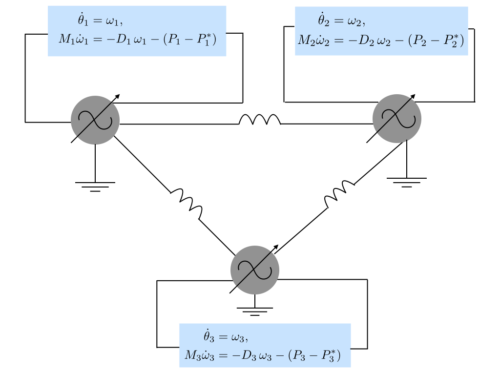
Refer to caption — Fig. 1: Three inverter system with dynamics given in (18), where $P_{i}=\sum_{j\in\mathcal{N}_{i}}b_{ij}\sin(\theta_{ij})$ and $P^{*}_{i}=\sum_{j\in\mathcal{N}_{i}}b_{ij}\sin(\theta^{*}_{ij})$ for $i=1,2,3$ .

We adopt the same setup as in [9] and consider a network of three inverters with system dynamics (18). The parameters $M_{i}$ and $D_{i}$ represent inertia and damping coefficients. The inverters are connected by purely inductive transmission lines with line susceptance $b_{ij}>0$ as shown in Figure 1. We test numerically the derived optimal controller (22) for nominal $(w=0)$ and disturbance attenuation $(w\neq 0)$ settings. The disturbance $w=[w_{1},\dots,w_{n}]^{\top}\in\real^{n}$ models for e.g. DC-side generation and AC side fluctuations [15]. For simplicity, we set all line susceptances $b_{ij}$ to one per unit (p.u.). The parameters in (18) are chosen uniformly with $M_{1}=M_{2}=M_{3}=0.01\mathrm{[s^{2}/rad]}$ and $D_{1}=D_{2}=D_{3}=0.1\mathrm{[s/rad]}$ .

Time-domain simulations of the open-loop angle differences and frequencies of the three inverter system with the unforced inverter system (i.e., $u=0$ ) in (18) and the desired steady state angle differences $\delta^{*}=[0,0,0]^{\top}$ , starting at $\delta(0)=[0.02;0.015,0,0]$ show that $\delta^{s}=[0.0113,0.0113,-0.0113]$ and thus satisfy Assumption 1. Moreover, the inverters frequencies synchronize at $\omega^{*}=0$ .

Next, we consider the optimal control problem (III-A) and implement the control law (22) both for nominal $(w=0)$ and disturbance attenuation $(w\neq 0)$ . We additionally verify the optimal controller for two examples of the design matrix $R_{1}$ and $R_{2}$ . Once in closed-loop with the optimal controller (22), all frequencies synchronize at nominal with a decay towards zero and improved transient behavior both for $R_{1}=0.1\cdot I_{3}$ and $R_{2}=0.01\cdot I_{3}$ in Figures 2 and 3 respectively. Compared to the input matrix $R_{1}$ , the matrix $R_{2}$ penalizes less the input variations and thus allows for more control input effort leading to faster error decay rate. In the presence of non-zero, additive and randomly generated disturbances $w=[w_{3},w_{2},w_{1}]^{\top}$ , Figure 4 shows that the frequencies remain bounded, albeit non-synchronized, which is in accordance with our theory. The nominal and disturbed cost functions are decreasing towards a value that is nearby zero.

Fig. 2: Simulations for

w=0

of angle differences, frequencies, inputs and the cost function of the three inverter system described in Figure 1 for

w=0

after closing the loop with the optimal control (22) with

R_{1}=0.1\cdot I_{3}

. The angles are stabilized at the specified steady state and the frequencies synchronize and decay towards zero. The cost function

L(\delta,\omega,R_{1})

strictly decreases towards a nearby zero value.

Fig. 3: Simulations for

w=0

of angle differences, frequencies, inputs and the cost function after closing the loop with the optimal control (22) for

R_{2}=0.1\cdot R_{1}

. The error decay transients of the angles and frequencies improve significantly with more control effort (compared to Figure 2). The nominal cost function

L(\delta,\omega,R_{2})

decays towards a nearby zero value.

Fig. 4: Simulations of the frequencies, input and cost function of the three-inverter system for constant non-zero disturbance

w

in closed-loop with (22) for

R=0.01\cdot I_{3},\,S=I_{3}

and

\xi=2.8>\frac{1}{4\,D}

. The frequencies remain bounded and the cost function

L(\delta,\omega,w,R,S)

in (1) takes negative values with a randomly generated disturbance

w\neq w^{*}(x)

IV Conclusion

We studied the role of cost design for optimal feedback control in satisfying HJBE or HJIE in theory and via examples and an application to control of oscillatory systems. The optimal control problem reduces to a decision on how to tune the control gains, while the value function remains unchanged. The optimal controller is thus comparable to a linear quadratic regulator. It is in our future interest to investigate the ramifications of the proposed design method on the study of passive systems and constrained optimal control problems.

References

[1] M. Sassano and A. Astolfi, “Combining Pontryagin’s Principle and dynamic programming for linear and nonlinear systems,” IEEE Transactions on Automatic Control, vol. 65, no. 12, pp. 5312–5327, 2020.
[2] D. P. Bertsekas, “Dynamic programming and optimal control 3rd edition, volume ii,” Belmont, MA: Athena Scientific, 2011.
[3] D. Liberzon, Calculus of variations and optimal control theory: a concise introduction. Princeton University Press, 2011.
[4] D. L. Lukes, “Optimal regulation of nonlinear dynamical systems,” SIAM Journal on Control, vol. 7, no. 1, pp. 75–100, 1969.
[5] W. B. Powell, Approximate Dynamic Programming: Solving the curses of dimensionality. John Wiley & Sons, 2007, vol. 703.
[6] C. Scherer, “Theory of robust control,” Delft University of Technology, pp. 1–160, 2001.
[7] K. Zhou and J. C. Doyle, Essentials of robust control. Prentice hall Upper Saddle River, NJ, 1998, vol. 104.
[8] T. Başar and P. Bernhard, H-infinity optimal control and related minimax design problems: a dynamic game approach. Springer Science & Business Media, 2008.
[9] T. Jouini and E. Tegling, “Optimal control for power converters based on phase angle feedback,” arXiv preprint arXiv:2101.11141, 2021.
[10] E. D. Sontag, Control-Lyapunov functions. London: Springer London, 1999, pp. 211–216.
[11] R. Vinter, Optimal control. Springer Science & Business Media, 2010.
[12] P. Monshizadeh, C. De Persis, T. Stegink, N. Monshizadeh, and A. van der Schaft, “Stability and frequency regulation of inverters with capacitive inertia,” in 2017 IEEE 56th Annual Conference on Decision and Control (CDC). IEEE, 2017, pp. 5696–5701.
[13] F. Dörfler and F. Bullo, “Synchronization and transient stability in power networks and nonuniform kuramoto oscillators,” SIAM Journal on Control and Optimization, vol. 50, no. 3, pp. 1616–1642, 2012.
[14] H. K. Khalil, Nonlinear systems, 3rd ed. Prentice hall New Jersey, 2002.
[15] P. Kundur, J. Paserba, V. Ajjarapu, G. Andersson, A. Bose, C. Canizares, N. Hatziargyriou, D. Hill, A. Stankovic, C. Taylor, et al., “Definition and classification of power system stability,” IEEE transactions on Power Systems, vol. 19, no. 2, pp. 1387–1401, 2004.

On cost design in applications of optimal control

Abstract

Index Terms:

I Introduction

II Main result

II-A Cost design for optimal control

Theorem II.1.

Proof.

Remark 1.

II-B Cost design for ℋ∞−\mathcal{H}_{\infty}-control

Proposition II.2.

Proof.

Remark 2.

III Application

III-A Optimal control of coupled oscillators

Assumption 1 ([12]).

Corollary III.1.

Proof.

III-B Simulations

IV Conclusion

References

II-B Cost design for $\mathcal{H}_{\infty}-$ control