跳到论文正文
W Papers独立论文阅读器 arXiv:2104.00661 论文正文 计算阅读时间 · 0%
引用这篇论文根据当前论文元数据生成,正式投稿前建议核对。


License: arXiv.org perpetual non-exclusive license
arXiv:2104.00661v2 [math.PR] 12 Apr 2021

Upper-tail Large Deviation Principle for the ASEP

Sayan Das Address: S. Das, Department of Mathematics, Columbia University,
  S. Das 2990 Broadway, New York, NY 10027 USA
Email address: sayan.das@columbia.edu
and Weitao Zhu Address: W. Zhu, Department of Mathematics, Columbia University,
  S. Das 2990 Broadway, New York, NY 10027 USA
Email address: weitao.zhu@columbia.edu
Abstract.

We consider the asymmetric simple exclusion process (ASEP) on ℤ\mathbb{Z} started from step initial data and obtain the exact Lyapunov exponents for H0​(t)H_{0}(t), the integrated current of ASEP. As a corollary, we derive an explicit formula for the upper-tail large deviation rate function for −H0​(t)-H_{0}(t). Our result matches with the rate function for the integrated current of the totally asymmetric simple exclusion process (TASEP) obtained in [Joh00].

Key words and phrases: 
ASEP, Lyapunov exponents, large deviations, Fredholm determinants.
2010 Mathematics Subject Classification
Primary 60F10, Secondary 82C22.

1. Introduction

1.1. The ASEP and main results

In this paper, we study the upper-tail Large Deviation Principle (LDP) of the asymmetric simple exclusion process (ASEP) with step initial data. The ASEP is a continuous-time Markov chain on particle configurations x=(x1>x2>⋯)\textbf{x}=(\textbf{x}_{1}>\textbf{x}_{2}>\cdots) in ℤ\mathbb{Z}. The process can be described as follows. Each site i∈ℤi\in\mathbb{Z} can be occupied by at most one particle, which has an independent exponential clock with exponential waiting time of mean 11. When the clock rings, the particle jumps to the right with probability qq or to the left with probability p=1−qp=1-q. However, the jump is only permissible when the target site is unoccupied. For our purposes, it suffices to consider configurations with a rightmost particle. At any time t∈ℝ>0t\in\mathbb{R}_{>0}, the process has the configuration x⁡(t)=(x1​(t)>x2​(t)>⋯)x(t)=(x_{1}(t)>x_{2}(t)>\cdots) in ℤ\mathbb{Z}, where xj​(t)x_{j}(t) denotes the location of the jj-th rightmost particle at this time. Appearing first in the biology work of Macdonald, Gibbs, and Pipkin [MGP68] and introduced to the mathematics community two years later by [Spi70], the ASEP has since become the “default stochastic model to study transport phenomena”, including mass transport, traffic flow, queueing behavior, driven lattices and turbulence. We refer to [BCS14, Lig05, Lig13, Spo91] for the mathematical study of and related to the ASEP.

When q=1,q=1, we obtain the totally asymmetric simple exclusion process (TASEP), which allows jumps only to the right. It connects to several other physical systems such as the exponential last-passage percolation, zero-temperature directed polymer in a random environment, the corner growth process and is known to possess complete determinantal structure (free-fermionicity). We refer the readers to [Joh00, Lig05, Lig13, PS02] and the references therein for more thorough treatises of the TASEP.

The dynamics of ASEP are uniquely determined once we specify its initial state. In the present paper, we restrict our attention to the ASEP started from the step initial configuration, i.e. xj​(0)=−jx_{j}(0)=-j, j=1,2,…j=1,2,\ldots. We set γ=q−p\gamma=q-p and assume q>12q>\frac{1}{2}, i.e., ASEP has a drift to the right. An observable of interest in ASEP is H0​(t)H_{0}(t), the integrated current through 0 which is defined as:

(1.1) H0​(t):= the number of particles to the right of zero at time ​t.\displaystyle H_{0}(t):=\mbox{ the number of particles to the right of zero at time }t.

H0​(t)H_{0}(t) can also be interpreted as the one-dimensional height function of the interface growth of the ASEP and thus carries significance in the broader context of the Kardar-Parisi-Zhang (KPZ) universality class. We will elaborate on the connection to KPZ universality class later in Section 1.3. As a well-known random growth model itself, the large-time behaviors of ASEP with step initial conditions have been well-studied. Indeed, it is known [Lig05, Chapter VIII, Theorem 5.12] that the current satisfies the following strong law of large numbers:

1t​H0​(tγ)→14, almost surely as ​t→∞.\displaystyle\tfrac{1}{t}{H_{0}\big(\tfrac{t}{\gamma}\big)}\rightarrow\tfrac{1}{4},\mbox{ almost surely as }t\to\infty.

The strong law has been later complemented by fluctuation results in the seminal works by Tracy and Widom. In a series of papers [TW08a], [TW08b] [TW09], Tracy and Widom exploit the integrability of ASEP with step initial data and establish via contour analysis that H0​(t)H_{0}(t) when centered by t4\frac{t}{4} has typical deviations of the order t1/3t^{1/3} and has the following asymptotic fluctuations:

(1.2) 1t1/3​24/3​(−H0​(tγ)+t4)⟹ξGUE,\displaystyle{\tfrac{1}{t^{1/3}}2^{4/3}\big(-H_{0}\big(\tfrac{t}{\gamma}\big)+\tfrac{t}{4}\big)\implies\xi_{\operatorname{GUE}},}

where ξGUE\xi_{\operatorname{GUE}} is the GUE Tracy-Widom distribution [TW94]. When q=1q=1, (1.2) recovers the same result on TASEP, which has been proved earlier by [Joh00].

Given the existing fluctuation results on the ASEP with step initial data, it is natural to inquire into its Large Deviation Principle (LDP). Namely, we seek to find the probability of when the event −H0​(tγ)+t4-H_{0}(\frac{t}{\gamma})+\frac{t}{4} has deviations of order tt. Intriguingly, one expects the lower- and upper-tail LDPs to have different speeds: the upper-tail deviation is expected to occur at speed tt whereas the lower-tail has speed t2t^{2}:

(Lower Tail) ℙ⁡(−H0​(tγ)+t4<−t4​y)≈e−t2​Φ−​(y);\displaystyle{\mathbb{P}\left(-H_{0}\big(\tfrac{t}{\gamma}\big)+\tfrac{t}{4}<-\tfrac{t}{4}y\right)\approx e^{-t^{2}\Phi_{-}(y)};}
(Upper Tail) ℙ⁡(−H0​(tγ)+t4>+t4​y)≈e−t​Φ+​(y).\displaystyle{\mathbb{P}\left(-H_{0}\big(\tfrac{t}{\gamma}\big)+\tfrac{t}{4}>+\tfrac{t}{4}y\right)\approx e^{-t\Phi_{+}(y)}.}

Thus, the upper tail corresponds to ASEP being “too slow” while the lower tail corresponds to ASEP being “too fast”. Heuristically, we can make sense of such speed differentials. Because of the nature of the exclusion process, when a single particle is moving slower than the usual, it forces all the particles on the left of it to be automatically slower. Hence ASEP becomes slow if only one particle is moving slow. This event has probability of the order exp⁡(−O⁡(t))\exp(-O(t)). However, in order to ensure that there are many particles on the right side of origin (this corresponds to ASEP being fast), it requires a large number of particles to move fast simulatenously. This event is much more unlikely and happens with probability exp⁡(−O⁡(t2))\exp(-O(t^{2})).

In this article, we focus on the upper-tail deviations of the ASEP with step initial data and present the first proof of the ASEP upper-tail LDP on the complete real line. Consider ASEP with q∈(12,1)q\in(\frac{1}{2},1) and set p=1−qp=1-q and τ=p/q∈(0,1)\tau=p/q\in(0,1). Our first theorem computes the ssth-Lyapunov exponent of τH0​(t)\tau^{H_{0}(t)}, which is the limit of the logarithm of 𝔼⁡[τs​H0​(t)]\mathbb{E}[\tau^{sH_{0}(t)}] scaled by time:

Theorem 1.1.

For s∈(0,∞)s\in(0,\infty) we have

(1.3) limt→∞1t​log⁡𝔼⁡[τs​H0​(t)]=−hq​(s)=:−(q−p)​1−τs21+τs2.\displaystyle\lim_{t\to\infty}\frac{1}{t}\log\mathbb{E}[\tau^{sH_{0}(t)}]=-h_{q}(s)=:-(q-p)\frac{1-\tau^{\frac{s}{2}}}{1+\tau^{\frac{s}{2}}}.

It is well known (see Proposition 1.12 in [GL20] for example) that the upper-tail large deviation principle of the stochastic process log⁡τH0​(t)\log\tau^{H_{0}(t)} is the Legendre-Fenchel dual of the Lyapunov exponent in (1.3). Since τ<1\tau<1, as a corollary, we obtain the following upper-tail large deviation rate function for −H0​(t)-H_{0}(t).

Theorem 1.2.

For any y∈(0,1)y\in(0,1) we have

(1.4) limt→∞1t​log⁡ℙ⁡(−H0​(tγ)+t4>t4​y)=−[y−(1−y)​tanh−1⁡(y)]=:−Φ+​(y),\displaystyle\lim_{t\to\infty}\frac{1}{t}\log\mathbb{P}\left(-H_{0}\big(\tfrac{t}{\gamma}\big)+\tfrac{t}{4}>\tfrac{t}{4}y\right)=-[\sqrt{y}-(1-y)\tanh^{-1}(\sqrt{y})]=:-\Phi_{+}(y),

where γ=2​q−1\gamma=2q-1. Furthermore, we have the following asymptotics near zero:

(1.5) limy→0+y−3/2Φ+(y)=23.\displaystyle\lim_{y\to 0^{+}}y^{-3/2}\Phi_{+}(y)=\tfrac{2}{3}.
Refer to caption

Refer to caption

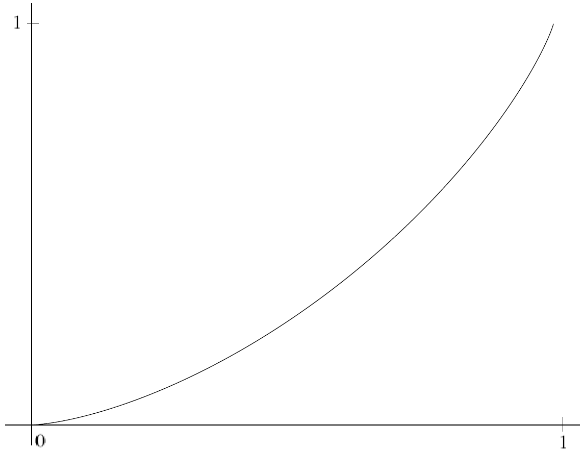
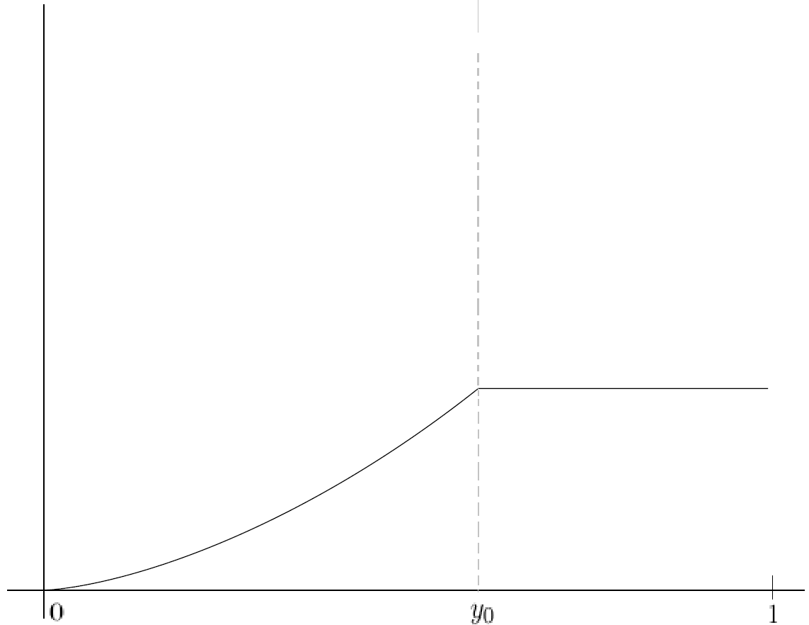
Figure 1. The figure on the left is the plot of Φ+​(y)\Phi_{+}(y). The right one is the plot of Φ~+​(y)\widetilde{\Phi}_{+}(y).
Remark 1.3.

Note that our large deviation result is restricted to y∈(0,1)y\in(0,1) as ℙ⁡(−H0​(tγ)+t4>t4​y)=0\mathbb{P}(-H_{0}\big(\tfrac{t}{\gamma}\big)+\tfrac{t}{4}>\tfrac{t}{4}y)=0 for y≥1y\geq 1. Furthermore, although Theorem 1.2 makes sense when q=1q=1, one cannot recover it from Theorem 1.1, which only makes sense for τ=(1−q)/q∈(0,1)\tau=(1-q)/q\in(0,1). However, as mentioned before, [Joh00] has already settled the q=1q=1 TASEP case and obtained the upper-tail rate function in a variational form. We will later show in Appendix A that [Joh00] variational formula for TASEP matches with our rate function in (1.4).

Remark 1.4.

Recently, the work [DPS18] has obtained a one-sided large deviation bound for the upper tail of the ASEP. In particular, they showed

(1.6) ℙ⁡(−H0​(tγ)+t4>t4​y)≤C​e−t​Φ~+​(y),y∈(0,1).\displaystyle\mathbb{P}\left(-H_{0}\big(\tfrac{t}{\gamma}\big)+\tfrac{t}{4}>\tfrac{t}{4}y\right)\leq\mathrm{C}e^{-t\widetilde{\Phi}_{+}(y)},\quad y\in(0,1).

The function Φ~+\widetilde{\Phi}_{+} coincides with the correct rate function Φ+\Phi_{+} defined in (1.4) only for y≤y0:=1−2​q⁡(1−q)1+2​q⁡(1−q)y\leq y_{0}:=\frac{1-2\sqrt{q(1-q)}}{1+2\sqrt{q(1-q)}}, as captured by Figure 1. We will further compare and contrast our results and method with [DPS18] later in Section 1.3.

Remark 1.5.

For yy small enough, following (1.2) and upper tail decay of GUE Tracy-Widom distribution [DV13], one expects

ℙ(−H0(tγ)+t4>t4y)≈ℙ(ξGUE>2−2/3yt2/3)≈e−23​y3/2​t\mathbb{P}\left(-H_{0}\big(\tfrac{t}{\gamma}\big)+\tfrac{t}{4}>\tfrac{t}{4}y\right)\approx\mathbb{P}(\xi_{\operatorname{GUE}}>2^{-2/3}yt^{2/3})\approx e^{-\frac{2}{3}y^{3/2}t}

Thus the asymptotics in (1.5) shows that Φ+​(y)\Phi_{+}(y) indeed recovers the expected GUE Tracy-Widom tails as y→0+y\to 0^{+}.

1.2. Sketch of proof

In this section we present a sketch of the proof of our main results. As explained before, Theorem 1.2 can be obtained from Theorem 1.1 by standard Legendre-Fenchel transform technique. So here we only give a brief account of the proof idea of Theorem 1.1. A more detailed overview of the proofs of our main results can be found in Section 2.

The main component of our proof is the following τ\tau-Laplace transform formula for H0​(t){H_{0}(t)} that appears in Theorem 5.3 in [BCS14]:

Theorem 1.6 (Theorem 5.3 in [BCS14]).

Fix any δ∈(0,1)\delta\in(0,1). For ζ>0\zeta>0 we have

(1.7) 𝔼⁡[Fq​(ζ​τH0​(t))]=det(I+Kζ,t),Fq​(ζ):=∏n=0∞11+ζ​τn.\displaystyle\mathbb{E}\left[F_{q}(\zeta\tau^{H_{0}(t)})\right]=\det(I+K_{\zeta,t}),\quad F_{q}(\zeta):=\prod_{n=0}^{\infty}\frac{1}{1+\zeta\tau^{n}}.

Here det(I+Kζ,t)\det(I+K_{\zeta,t}) is the Fredholm determinant of Kζ,t:L2​(ℭ⁡(τ1−δ2))→L2​(ℭ⁡(τ1−δ2)),K_{\zeta,t}:L^{2}(\mathfrak{C}(\tau^{1-\frac{\delta}{2}}))\rightarrow L^{2}(\mathfrak{C}(\tau^{1-\frac{\delta}{2}})), and ℭ⁡(τ1−δ2)\mathfrak{C}(\tau^{1-\frac{\delta}{2}}) denotes a positively-oriented circular contour centered at 0 with radius τ1−δ2.\tau^{1-\frac{\delta}{2}}. The operator Kζ,tK_{\zeta,t} is defined through the integral kernel

(1.8) Kζ,t​(w,w′)\displaystyle K_{\zeta,t}(w,w^{\prime}) :=12​π​𝐢​∫δ−𝐢​∞δ+𝐢​∞Γ⁡(−u)​Γ​(1+u)​ζu​gt​(w)gt​(τu​w)​d​uw′−τu​w, for ​gt​(z)=exp⁡((q−p)​t1+zτ).\displaystyle:=\frac{1}{2\pi\mathbf{i}}\int\limits_{\delta-\mathbf{i}\infty}^{\delta+\mathbf{i}\infty}\Gamma(-u)\Gamma(1+u)\zeta^{u}\frac{g_{t}({w})}{g_{t}({\tau^{u}w})}\frac{\mathrm{d}u}{w^{\prime}-\tau^{u}w},\ \mbox{ for }g_{t}(z)=\exp\left(\frac{(q-p)t}{1+\frac{z}{\tau}}\right).
Remark 1.7.

The original statement of the above theorem in [BCS14] appears in a much more general setup with general conditions on the contours. We will explain the choice of our contours stated above in Section 3 and check that it satisfies the general criterion for contours as stated in Theorem 5.3 in [BCS14].

We next recall that the Fredholm determinant is defined as a series as follows.

(1.9) det(I+Kζ,t)\displaystyle\det(I+K_{\zeta,t}) :=1+∑L=1∞tr⁡(Kζ,t∧L)\displaystyle:=1+\sum_{L=1}^{\infty}\mathrm{tr}(K_{\zeta,t}^{\wedge L})
(1.10) :=1+∑L=1∞1L!∫ℭ⁡(τ1−δ2)⋯∫ℭ⁡(τ1−δ2)det(Kζ,t(wi,wj))i,j=1L∏i=1Ldwi.\displaystyle:=1+\sum_{L=1}^{\infty}\frac{1}{L!}\int_{\mathfrak{C}(\tau^{1-\frac{\delta}{2}})}\cdots\int_{\mathfrak{C}(\tau^{1-\frac{\delta}{2}})}\det(K_{\zeta,t}(w_{i},w_{j}))_{i,j=1}^{L}\prod_{i=1}^{L}\mathrm{d}w_{i}.

The notation Kζ,t∧LK_{\zeta,t}^{\wedge L} comes from the exterior algebra definition, which we refer to [Sim77] for more details. As a clarifying remark, we use this exterior algebra notation only for the simplicity of its expression and rely essentially on the definition in (1.10) throughout the rest of the paper.

To extract information on the fractional moments of τH0​(t)\tau^{H_{0}(t)}, we combine the formula in (1.7) with the following elementary identity, which is a generalized version of Lemma 1.4 in [DT19].

Lemma 1.8.

Fix n∈ℤ>0n\in\mathbb{Z}_{>0} and α∈[0,1)\alpha\in[0,1). Let UU be a nonnegative random variable with finite nn-th moment. Let F:[0,∞)→[0,1]F:[0,\infty)\to[0,1] be a nn-times differentiable function such that ∫0∞ζ−α​F(n)​(ζ)​𝑑ζ\int_{0}^{\infty}\zeta^{-\alpha}F^{(n)}(\zeta)\mathrm{d}\zeta is finite. Assume further that ‖F(k)‖∞<∞\|F^{(k)}\|_{\infty}<\infty for all 1≤k≤n1\leq k\leq n. Then the (n−1+α)(n-1+\alpha)-th moment of UU is given by

𝔼⁡[Un−1+α]=∫0∞ζ−α​𝔼​[Un​F(n)​(ζ​U)]​𝑑ζ∫0∞ζ−α​F(n)​(ζ)​𝑑ζ=∫0∞ζ−α​dnd​ζn​𝔼​[F⁡(ζ​U)]​𝑑ζ∫0∞ζ−α​F(n)​(ζ)​𝑑ζ.\displaystyle\mathbb{E}[U^{n-1+\alpha}]=\dfrac{\int\limits_{0}^{\infty}\zeta^{-\alpha}\mathbb{E}[U^{n}F^{(n)}(\zeta U)]\mathrm{d}\zeta}{\int\limits_{0}^{\infty}\zeta^{-\alpha}F^{(n)}(\zeta)\mathrm{d}\zeta}=\dfrac{\int\limits_{0}^{\infty}\zeta^{-\alpha}\frac{\mathrm{d}^{n}}{\mathrm{d}\zeta^{n}}\mathbb{E}[F(\zeta U)]\mathrm{d}\zeta}{\int\limits_{0}^{\infty}\zeta^{-\alpha}F^{(n)}(\zeta)\mathrm{d}\zeta}.

The proof of this lemma follows by an interchange of measure justified by Fubini’s theorem and the dominated convergence theorem, as 𝔼⁡[Un]\mathbb{E}[U^{n}] and ‖F(k)‖∞<∞\|F^{(k)}\|_{\infty}<\infty for all 1≤k≤n.1\leq k\leq n.

For s>0s>0, we apply this lemma with U=τH0​(t)U=\tau^{H_{0}(t)}, n=⌊s⌋+1n=\lfloor s\rfloor+1 and α=s−⌊s⌋\alpha=s-\lfloor s\rfloor. We take F​(x)=Fq​(x)F(x)=F_{q}(x) defined in (1.7) which is shown to be satisfy the hypothesis of Lemma 1.8 (see Proposition 2.2). As a result, we transform the computation of 𝔼⁡[τs​H0​(t)]\mathbb{E}[\tau^{sH_{0}(t)}] into that of

(1.11) ∫0∞ζ−α​dnd​ζn​𝔼​[Fq​(ζ​τH0​(t))]​𝑑ζ.\displaystyle\int_{0}^{\infty}\zeta^{-\alpha}\frac{\mathrm{d}^{n}}{\mathrm{d}\zeta^{n}}\mathbb{E}[F_{q}(\zeta\tau^{H_{0}(t)})]\mathrm{d}\zeta.

Utilizing the exact formula from (1.7) and the definition of Fredholm determinant from (1.10), we can write the above expression as a series where we identify the leading term (corresponding to L=1L=1 term of the series) and a higher-order term (corresponding to L≥2L\geq 2 terms of the series). We eventually show that the asymptotics of the leading term matches with the exact asymptotics in (1.3) while the higher-order term decays much faster. This leads to the proof of Theorem 1.1.

The above description of our method is in line with the Lyapunov moment approach adopted in the works of [DT19], [GL20] and [Lin20] to obtain upper-tail large deviation results of other integrable models, such as the KPZ equation. Namely, we extract fractional moments from the (τ\tau-)Laplace transform such as (1.7) according to Lemma 1.8. In particular, our work draws from those of [DT19] and [Lin20], which studied the fractional moments of the Stochastic Heat Equation (SHE) and the half-line Stochastic Heat Equation, respectively. We will further contextualize the connections of our work to [DT19], [GL20] and [Lin20] in Section 1.3. In the following text, however, we emphasize a few key differences and technical challenges unique to the ASEP that we have encountered and resolved in our proof.

First, unlike SHE or half-line SHE, the usual Laplace transform is not available in case of the ASEP. Instead, we only have the τ\tau-Laplace transform for our observable of interest. As a result, we have formulated Lemma 1.8 in our paper, which is more generalized than its prototype in [DT19, Lemma 1.4], to feed in the τ\tau-Laplace transform. Consequently, we have worked with τ\tau-exponential functions in our analysis.

Another key difference is that the kernel Kζ,tK_{\zeta,t} in (1.8) in our model is much more intricate than its counterpart in the KPZ model and leads to much more involved analysis of the leading term. Indeed, Kζ,tK_{\zeta,t} is asymmetric and as uu varies in (δ−𝐢​∞,δ+𝐢​∞)(\delta-\mathbf{i}\infty,\delta+\mathbf{i}\infty), the function gt​(w)gt​(τu​w)\frac{g_{t}(w)}{g_{t}(\tau^{u}w)} appearing in the kernel Kζ,tK_{\zeta,t}, exhibits a periodic behavior, whereas the kernel in the KPZ models involves Airy functions in its integrand which have a unique maximum and are much easier to analyze. Furthermore, our model exhibits exponentially decaying moments of τH0​(t)\tau^{H_{0}(t)} as opposed to the exponentially increasing ones of the KPZ models in [DT19] and [Lin20] and this demands a more precise understanding of the trace term of our Fredholm determinant expansion. For instance in Section 3, to obtain the precise asymptotics for our leading term, we have performed steepest descent analysis on the kernel Kζ,tK_{\zeta,t}, where the periodic nature of gt​(w)gt​(τu​w)\frac{g_{t}(w)}{g_{t}(\tau^{u}w)} results in infinitely many critical points. A major technical challenge in our proof is to argue how the contribution from only one of the critical points dominates the those from the rest and this is accomplished in the proof of Proposition 2.4. Similarly, the asymmetry of the kernel in the ASEP model has led us to opt for the Hadamard’s inequality approach as exemplified in Section 4 of [Lin20], instead of the operator theory argument in [DT19], to obtain a sufficient upper bound for the higher-order terms in our paper in Section 4.

1.3. Comparison to Previous Works

In a broader context, our main result on the Lyapunov exponent for the ASEP with step initial data and its upper-tail large deviation belongs to the undertakings of studying the intermittency phenomenon and large deviation problems of integrable models in the KPZ universality class. As we have previously alluded to, the KPZ universality class contains a collection of random growth models that are characterized by scaling exponent of 1/31/3 and certain universal non-Gaussian large time fluctuations. We refer to [ACQ11, Cor12, TS19] and the references therein for more details. The ASEP is one of the standard one-dimensional models of the KPZ universality class and bears connection to several other integrable models in this class, such as the stochastic six-vertex model [BCG16, Agg17, CD18], KPZ equation [CLDR10, Dot10, SS10, ACQ11, Cor12], and qq-TASEP [BCS14].

On the other hand, the intermittency property is a universal phenomenon that captures high population concentrations on small spatial islands over large time. Mathematically, the intermittency of a random field is defined in terms of its Lyapunov exponents. In particular, the connection between integer Lyapunov moments and intermittency has long been an active area of study in the SPDE community in last few decades [GM90, CM94, BC95, FK09, HHNT15, CJK13, CD15, BC16]. For the KPZ equation, [Kar87] predicted the integer Lyapunov exponents for the SHE using replica Bethe anstaz techniques. This result was later first rigorously attempted in [BC95] and correctly proven in [Che15]. Similar formulas were shown for the moments of the parabolic Anderson model, semi-discrete directed polymers, q-Whittaker process (see [BC14a] and [BC14b]). For the ASEP, integer moments formula for τH0​(t)\tau^{H_{0}(t)} were obtained in [BCS14] using nested contour integral ansatz.

From the perspective of tail events, by studying the asymptotics of integer Lyapunov exponents formulas, one can extract one-sided bounds on the upper tails of integrable models. However, these integer Lyapunov exponents alone are not sufficient to provide the exact large deviation rate function.

Recently, a stream of effort has been devoted to studying large deviations for some KPZ class models by explicitly computing the fractional Lyapunov exponents. The work of [DT19] set this series of effort in motion by solving the KPZ upper-tail large deviation principle through the fractional Lyapunov exponents of the SHE with delta initial data. [GL20] soon extended the same result for the SHE for a large class of initial data, including any random bounded positive initial data and the stationary initial data. An exact way to compute every positive Lyapunov exponent of the half-line SHE was also uncovered in [Lin20]. In lieu of these developments, our main result for the ASEP with step initial data and its upper-tail large deviation fits into this broader endeavor of studying large deviation problems of integrable models with the Lyapunov exponent appproach.

Meanwhile, in the direction of the ASEP, as mentioned before, [DPS18] has produced a one-sided large deviation bound for the upper-tail probability appearing in (1.4) which coincides with the correct rate function Φ+\Phi_{+} defined in (1.4) for y≤y0:=1−2​q⁡(1−q)1+2​q⁡(1−q)y\leq y_{0}:=\frac{1-2\sqrt{q(1-q)}}{1+2\sqrt{q(1-q)}}. This result was sufficient for their purpose of establishing a near-exponential fixation time for the coarsening model on ℤ2\mathbb{Z}^{2} and [DPS18] obtained it via steepest descent analysis on the exact formula for the probability of H0​(t/γ)H_{0}(t/\gamma). More specially, they worked with the following result from [TW09, Lemma 4] as input:

(1.12) ℙ⁡(−H0​(tγ)+t4>t4​y)=12​π​𝐢​∫|μ|=R(μ,τ)∞​det(1+μ​Jm,t(μ))​d​μμ,\mathbb{P}\left(-H_{0}\big(\tfrac{t}{\gamma}\big)+\tfrac{t}{4}>\tfrac{t}{4}y\right)=\frac{1}{2\pi\mathbf{i}}\int_{|\mu|=R}(\mu;\tau)_{\infty}\det(1+\mu J_{m,t}^{(\mu)})\frac{\mathrm{d}\mu}{\mu},

where m=⌊14​t​(1−y)⌋m=\lfloor\frac{1}{4}t(1-y)\rfloor, R∈(τ,∞)∖{1,τ−1,τ−2,…}R\in(\tau,\infty)\setminus\{1,\tau^{-1},\tau^{-2},\ldots\} is fixed, (μ,τ)∞:=(1−μ)​(1−μ​τ)​(1−μ​τ2)​…(\mu;\tau)_{\infty}:=(1-\mu)(1-\mu\tau)(1-\mu\tau^{2})\ldots is the infinite τ\tau-Pochhammer symbol and Jm,t(μ)J_{m,t}^{(\mu)} is the kernel defined in Equation (3.4) of [DPS18]. Analyzing the exact pre-limit Fredholm determinant det(1+μ​Jm,t(μ))\det(1+\mu J_{m,t}^{(\mu)}), [DPS18] chose appropriate contours for the kernel Jm,t(μ)J_{m,t}^{(\mu)} that pass through its critical points and performed a steepest descent analysis. However, their choice of contours was unattainable beyond the threshold y0y_{0}. Namely, if we attempted to deform the same contours for y>y0y>y_{0}, we would inevitably cross poles, which rendered the steepest descent analysis much trickier. By adopting the Lyapunov moment approach, we have avoided this problem when looking for the precise large deviation rate function.

In addition to the relavence of our upper-tail LDP result, it is also worthy to remark on the difficulty of obtaining a lower-tail LDP of the ASEP with step initial data. As explained before, the lower-tail ℙ⁡(−H0​(tγ)+t4<−t4​y)\mathbb{P}(-H_{0}\big(\tfrac{t}{\gamma}\big)+\tfrac{t}{4}<-\tfrac{t}{4}y) is expected to go to zero at a much faster rate of exp⁡(−t2​Φ−​(y))\exp(-t^{2}\Phi_{-}(y)). The existence of the lower-tail rate function has so far only been shown in the case of TASEP in [Joh00] through its connection to continuous log-gases. The functional LDPs for TASEP for both tails have been studied in [Jen00], [Var04], [QT21] (upper tail), and [OT19] (lower-tail). Large deviations for open systems with boundaries in contact with stochastic reservoirs has also been studied in physics literature. We mention [DL98], [DLS03], [BD05] and the references therein for works in these directions.

More broadly for integrable models in the KPZ universality class, lower tail of the KPZ equation has been extensively studied in both mathematics and physics communities. In the physics literature, [LDMS16a] provided the first prediction of the large deviation tails of the KPZ equation for narrow wedge initial data. For the upper tail, their analysis also yields subdominant corrections ([LDMS16b, Supp. Mat.]). Furthermore, the physics work of [SMP17] first predicted lower-tail rate function of the KPZ equation for narrow wedge initial data in an analytical form, followed by the derivations in [CGK+18] and [KLDP18] via different methods. The asymptotics of deep lower tail of KPZ equation was later obtained in [KLD18b] for a wide class of initial data. From the mathematics front, the work [CG20] provided detailed, rigorous tail bounds for the lower tail of the KPZ equation for narrow wedge initial data. The precise rate function of its lower-tail LDP was later proved in [Tsa18] and [CC19], which confirmed the prediction of existing physics literature. The four different routes of deriving the lower-tail LDP in [SMP17], [CGK+18], [KLDP18] and [Tsa18] were later shown to be closely related in [KLD18a]. A new route has also been recently obtained in the physics work of [LD20] (see also [Pro20]).

In the short time regime, large deviations for the KPZ equation has been studied extensively in physics literature (see [LDMRS16], [KLD17], [Kra20] and the references therein for a review). Recently, [LT21] rigorously derived the large deviation rate function of the KPZ equation in the short-time regime in a variational form and recovered deep lower-tail asymptotics, confirming existing physics predictions. For non-integrable models, large deviations of first-passage percolation were studied in [CZ03] and more recently [BGS17]. For last-passage percolation with general weights, recently, geometry of polymers under lower tail large deviation regime has been studied in [BGS19].

Notation

Throughout the rest of the paper, we use C=C⁡(a,b,c,…)>0\mathrm{C}=\mathrm{C}(a,b,c,\ldots)>0 to denote a generic deterministic positive finite constant that is dependent on the designated variables a,b,c,…a,b,c,\ldots. However, its particular content may change from line to line. We also use the notation ℭ⁡(r)\mathfrak{C}(r) to denote a positively oriented circle with center at origin and radius r>0r>0.

Outline

The rest of this article is organized as follows. In Section 2, we introduce the main ingredients for the proofs of Theorem 1.1 and 1.2. In particular, we reduce the proof of our main results to Proposition 2.4 (asymptotics of the leading order) and Proposition 2.5 (estimates for the higher order), which are proved in Sections 3 and 4 respectively. Finally, in Appendix A we compare our rate function Φ+​(y)\Phi_{+}(y), defined in (1.4), to that of TASEP.

Acknowledgements

We are grateful to Ivan Corwin for suggesting the problem and providing numerous stimulating discussions. His encouragement and inputs on earlier drafts of the paper have been invaluable. We also thank Evgeni Dimitrov, Li-Cheng Tsai, Yier Lin and Mark Rychnovsky for helpful conversations and Pierre Le Doussal and Alexandre Krajenbrink for providing many valuable references to the physics literature. The authors were partially supported by Ivan Corwin’s NSF grant DMS:1811143 as well as the Fernholz Foundation’s “Summer Minerva Fellows” program.

2. Proof of Main Results

In this section, we give a detailed outline of the proofs of Theorems 1.1 and 1.2. In Section 2.1 we collect some useful properties of hqh_{q} and FqF_{q} functions defined in (1.4) and (1.7) respectively. In Section 2.2 we complete the proof of Theorems 1.1 and 1.2 assuming technical estimates on the leading order term (Proposition 2.4) and higher order term (Proposition 2.5).

Throughout this paper, we fix s>0s>0 and set n=⌊s⌋+1≥1n=\lfloor s\rfloor+1\geq 1 and α=s−⌊s⌋\alpha=s-\lfloor s\rfloor so that s=n−1+αs=n-1+\alpha. We also fix q∈(12,1)q\in(\frac{1}{2},1) and set p=1−qp=1-q and τ=p/q∈(0,1)\tau=p/q\in(0,1) for the rest of the article.

2.1. Properties of hq​(x)h_{q}(x) and Fq​(x)F_{q}(x)

Recall the Lyapunov exponent hq​(x)h_{q}(x) defined in (1.3) and the Fq​(x)F_{q}(x) function defined in (1.7). The following two propositions investigates various properties of these two functions which are necessary for our later proofs.

Proposition 2.1 (Properties of hqh_{q}).

Consider the function hq:(0,∞)→ℝh_{q}:(0,\infty)\to\mathbb{R} defined by hq​(x)=(q−p)​1−τx21+τx2h_{q}(x)=(q-p)\frac{1-\tau^{\frac{x}{2}}}{1+\tau^{\frac{x}{2}}}. Then, the following properties hold true:

  1. (a)

    Bq​(x):=hq​(x)xB_{q}(x):=\frac{h_{q}(x)}{x} is strictly positive and strictly decreasing with

    limx→0+Bq​(x)=14​(p−q)​log⁡τ>0.\lim_{x\to 0^{+}}B_{q}(x)=\tfrac{1}{4}(p-q)\log\tau>0.
  2. (b)

    hqh_{q} is strictly subadditive in the sense that for any x,y∈(0,∞)x,y\in(0,\infty) we have

    hq​(x+y)<hq​(x)+hq​(y).h_{q}(x+y)<h_{q}(x)+h_{q}(y).
  3. (c)

    hqh_{q} is related to Φ+\Phi_{+} defined in (1.4) via the following Legendre-Fenchel type transformation:

    Φ+​(y)=sups∈ℝ>0{s​1−y4​log⁡τ+1q−p​hq​(s)},y∈(0,1).\displaystyle\Phi_{+}(y)=\sup_{s\in\mathbb{R}_{>0}}\left\{s\frac{1-y}{4}\log\tau+\frac{1}{q-p}h_{q}(s)\right\},\quad y\in(0,1).
Proof.

For (a), first, the positivity of Bq​(x)B_{q}(x) follows from the positivity of hq​(x).h_{q}(x). To see its growth, taking the derivative of Bq​(x)B_{q}(x) we obtain

(2.1) Bq′​(x)=(q−p)​(−x​τx2​log⁡τ−1+τx)(1+τx2)2​x2.\displaystyle B_{q}^{\prime}(x)=\frac{(q-p)(-x\tau^{\frac{x}{2}}\log\tau-1+\tau^{x})}{(1+\tau^{\frac{x}{2}})^{2}x^{2}}.

Note that the numerator on the r.h.s of (2.1) is 0 when x=0x=0 and its derivative against xx is τx2​log⁡τ⁡(τx2−x2​log⁡τ−1)<0\tau^{\frac{x}{2}}\log\tau(\tau^{\frac{x}{2}}-\frac{x}{2}\log\tau-1)<0 for x>0x>0. Thus Bq′​(x)B_{q}^{\prime}(x) is strictly negative when x>0x>0 and Bq​(x)B_{q}(x) is strictly decreasing for x>0x>0. L’Hôpital’s rule yields that limx→0+Bq​(x)=hq′​(0)=14​(q−p)​log⁡τ.\lim_{x\to 0^{+}}B_{q}(x)=h_{q}^{\prime}(0)=\frac{1}{4}(q-p)\log\tau.

For (b), direct computation yields

(2.2) hq​(x+y)−hq​(x)−hq​(y)=−(q−p)​(1−τy2)​(1−τx2)​(1−τx+y2)(1+τx+y2)​(1+τx2)​(1+τy2)<0.\displaystyle h_{q}(x+y)-h_{q}(x)-h_{q}(y)=-(q-p)\frac{(1-\tau^{\frac{y}{2}})(1-\tau^{\frac{x}{2}})(1-\tau^{{\frac{x+y}{2}}})}{(1+\tau^{{\frac{x+y}{2}}})(1+\tau^{{\frac{x}{2}}})(1+\tau^{{\frac{y}{2}}})}<0.

Lastly, for part (c), we fix y∈(0,1)y\in(0,1) and define

gy​(s):=s​1−y4​log⁡τ+1q−p​hq​(s),s>0.\displaystyle g_{y}(s):=s\frac{1-y}{4}\log\tau+\frac{1}{q-p}h_{q}(s),\quad s>0.

Direct computation yields gy′​(s)=(1−y4−τs2(1+τs2)2)​log⁡τg_{y}^{\prime}(s)=(\frac{1-y}{4}-\frac{\tau^{\frac{s}{2}}}{(1+\tau^{\frac{s}{2}})^{2}})\log\tau and gy′′​(s)=τs2​(τs2−1)​log2​τ2​(1+τs2)3<0g_{y}^{\prime\prime}(s)=\frac{\tau^{\frac{s}{2}}(\tau^{\frac{s}{2}}-1)\log^{2}\tau}{2(1+\tau^{\frac{s}{2}})^{3}}<0. Thus gy​(s)g_{y}(s) is concave on (0,∞)(0,\infty) and hence attains its unique maxima when gy′​(s)=0g_{y}^{\prime}(s)=0 or equivalently 1−y4=τs2(1+τs2)2.\frac{1-y}{4}=\frac{\tau^{\frac{s}{2}}}{(1+\tau^{\frac{s}{2}})^{2}}. The last equation has s=2​logτ​(1−y1+y)s=2\log_{\tau}(\frac{1-\sqrt{y}}{1+\sqrt{y}}) as the only positive solution and hence it defines the unique maximum. Substituting this ss back into gy​(s)g_{y}(s) generates the final result as Φ+​(y).\Phi_{+}(y). ∎

Proposition 2.2 (Properties of Fq​(ζ)F_{q}(\zeta)).

Consider the function Fq:[0,∞)→[0,1]F_{q}:[0,\infty)\to[0,1] defined by Fq​(ζ):=∏n=0∞(1+ζ​τn)−1F_{q}(\zeta):=\prod_{n=0}^{\infty}(1+\zeta\tau^{n})^{-1}. Then, the following properties hold true:

  1. (a)

    FqF_{q} is an infinitely differentiable function with (−1)n​Fq(n)​(ζ)≥0(-1)^{n}F_{q}^{(n)}(\zeta)\geq 0 for all x>0x>0. Furthermore, ‖Fq(n)‖∞<∞\|F_{q}^{(n)}\|_{\infty}<\infty for each nn.

  2. (b)

    For each n∈ℤ>0n\in\mathbb{Z}_{>0}, and α∈[0,1)\alpha\in[0,1), (−1)n​∫0∞ζ−α​Fq(n)​(ζ)​𝑑ζ(-1)^{n}\int_{0}^{\infty}\zeta^{-\alpha}F_{q}^{(n)}(\zeta)\mathrm{d}\zeta is positive and finite.

  3. (c)

    All the derivatives of FqF_{q} have superpolynomial decay. In other words for any m,n∈ℤ≥0m,n\in\mathbb{Z}_{\geq 0} we have

    supζ>0|ζm​Fq(n)​(ζ)|<∞.\sup_{\zeta>0}|\zeta^{m}F_{q}^{(n)}(\zeta)|<\infty.
Proof.

(a) Note that Fq​(ζ)=∏n=0∞(1+ζ​τn)−1=(−ζ,τ)∞−1F_{q}(\zeta)=\prod_{n=0}^{\infty}(1+\zeta\tau^{n})^{-1}=(-\zeta;\tau)_{\infty}^{-1} where we recall that (−ζ,τ)∞(-\zeta;\tau)_{\infty} is the τ\tau-Pochhammer symbol. As (−ζ,τ)∞(-\zeta;\tau)_{\infty} is analytic [AAR99, Corollary A.1.6.] and nonzero for ζ∈[0,∞),\zeta\in[0,\infty), its inverse Fq​(ζ)F_{q}(\zeta) is analytic.

We next rewrite Fq​(ζ)=∏n=0∞fn​(ζ),F_{q}(\zeta)=\prod_{n=0}^{\infty}f_{n}(\zeta), where fn​(ζ)=(1+ζ​τn)−1f_{n}(\zeta)=(1+\zeta\tau^{n})^{-1}. Denote H⁡(ζ):=log⁡Fq​(ζ).H(\zeta):=\log F_{q}(\zeta). Since each fn​(ζ)∈(0,1)f_{n}(\zeta)\in(0,1) is analytic for ζ∈[0,∞)\zeta\in[0,\infty) and the product ∏n=0∞fn​(ζ)∈(0,1)\prod_{n=0}^{\infty}f_{n}(\zeta)\in(0,1) converges locally and uniformly, H⁡(ζ)H(\zeta) is well-defined and H⁡(ζ)=∑n=0∞log⁡fn​(ζ).H(\zeta)=\sum_{n=0}^{\infty}\log f_{n}(\zeta). Given that |∑n=0∞1fn​(ζ)​fn′​(ζ)|=∑n=0∞τn(1+ζ​τn)<11−τ,|\sum_{n=0}^{\infty}\frac{1}{f_{n}(\zeta)}f_{n}^{\prime}(\zeta)|=\sum_{n=0}^{\infty}\frac{\tau^{n}}{(1+\zeta\tau^{n})}<\frac{1}{1-\tau}, we have

(2.3) H′​(ζ)=Fq′​(ζ)Fq​(ζ)=∑n=1∞fn′​(ζ)fn​(ζ)=:G⁡(ζ).H^{\prime}(\zeta)=\frac{F_{q}^{\prime}(\zeta)}{F_{q}(\zeta)}=\sum_{n=1}^{\infty}\frac{f_{n}^{\prime}(\zeta)}{f_{n}(\zeta)}=:G(\zeta).

Note that G(ζ)=−∑j=1∞τjfj(ζ)G(\zeta)=-\sum_{j=1}^{\infty}\tau^{j}f_{j}(\zeta) and |G⁡(ζ)|<∞.|G(\zeta)|<\infty. For each m∈ℤ>0m\in\mathbb{Z}_{>0}, let us set G(m)(ζ):=−∑j=1∞τjfj(m)(ζ).G^{(m)}(\zeta):=-\sum_{j=1}^{\infty}\tau^{j}f_{j}^{(m)}(\zeta). As fj(m)​(ζ)=(−1)m​m!​τm​j(1+ξ​τj)m+1,f_{j}^{(m)}(\zeta)=(-1)^{m}m!\frac{\tau^{mj}}{(1+\xi\tau^{j})^{m+1}}, we obtain |G(m)​(ζ)|≤m!1−τm+1<∞|G^{(m)}(\zeta)|\leq\frac{m!}{1-\tau^{m+1}}<\infty converges locally and uniformly. Induction on mm gives us that G⁡(ζ)G(\zeta) is infinitely differentiable and the mm-th derivative of GG is G(m)G^{(m)}. It follows that Fq​(ζ)F_{q}(\zeta) is infinitely differentiable too. In particular, for any finite n∈ℤ≥0n\in\mathbb{Z}_{\geq 0}, by Leibniz’s rule on the relation (2.3) we obtain

(2.4) Fq(n+1)​(ζ)=∑k=0n(nk)​Fq(n−k)​(ζ)​G(k)​(ζ).\displaystyle F_{q}^{(n+1)}(\zeta)=\sum_{k=0}^{n}\binom{n}{k}F_{q}^{(n-k)}(\zeta)G^{(k)}(\zeta).

Observe that (−1)k+1​G(k)(-1)^{k+1}G^{(k)} is positive and finite. As FqF_{q} is positive and finite, using (2.4), induction gives us that (−1)n​Fq(n)(-1)^{n}F_{q}^{(n)} is also positive and finite. As ‖G(m)‖∞\|G^{(m)}\|_{\infty} and ‖Fq‖∞\|F_{q}\|_{\infty} are finite, using (2.4), induction gives us that ‖Fq(n)‖∞\|F_{q}^{(n)}\|_{\infty} is finite for any n∈ℤ≥0.n\in\mathbb{Z}_{\geq 0}.

(b) For α∈[0,1)\alpha\in[0,1), positivity of the integral (−1)n​∫0∞ζ−α​Fq(n)​(ζ)​𝑑ζ(-1)^{n}\int_{0}^{\infty}\zeta^{-\alpha}F_{q}^{(n)}(\zeta)\mathrm{d}\zeta follows from part (a). To check the integrability, we first verify the n=0n=0 case. Since ζ≥0\zeta\geq 0 and τ∈(0,1),\tau\in(0,1),

0<∫0∞ζ−α​Fq​(ζ)​𝑑ζ=∫0∞ζ−α​∏m=0∞11+ζ​τm​𝑑ζ<∫0∞ζ−α​11+ζ​𝑑ζ=∫01ζ−α​11+ζ​dζ+∫1∞d​ζζα​(1+ζ)<∫01ζ−α​dζ+∫1∞d​ζζα+1<∞.\begin{split}0&<\int_{0}^{\infty}\zeta^{-\alpha}F_{q}(\zeta)\mathrm{d}\zeta=\int_{0}^{\infty}\zeta^{-\alpha}\prod_{m=0}^{\infty}\frac{1}{1+\zeta\tau^{m}}\mathrm{d}\zeta<\int_{0}^{\infty}\zeta^{-\alpha}\frac{1}{1+\zeta}\mathrm{d}\zeta\\ &=\int_{0}^{1}\zeta^{-\alpha}\frac{1}{1+\zeta}\mathrm{d}\zeta+\int_{1}^{\infty}\frac{\mathrm{d}\zeta}{\zeta^{\alpha}(1+\zeta)}<\int_{0}^{1}\zeta^{-\alpha}\mathrm{d}\zeta+\int_{1}^{\infty}\frac{\mathrm{d}\zeta}{\zeta^{\alpha+1}}<\infty.\end{split}

When n>0n>0, using (2.4) and the fact the |G(m)​(ζ)|<m!1−τm+1|G^{(m)}(\zeta)|<\frac{m!}{1-\tau^{m+1}}, the finiteness of (−1)n​∫0∞ζ−α​Fq(n)​(ζ)​𝑑ζ(-1)^{n}\int_{0}^{\infty}\zeta^{-\alpha}F_{q}^{(n)}(\zeta)\mathrm{d}\zeta follows from induction.

(c) Clearly for each mm we have Fq​(ζ)≤1(1+ζ​τm)m+1F_{q}(\zeta)\leq\frac{1}{(1+\zeta\tau^{m})^{m+1}} forcing superpolynomial decay of FqF_{q}. The superpolynomial decay of higher order derivative now follows via induction using (2.4). ∎

2.2. Proof of Theorem 1.1 and Theorem 1.2

Recall H0​(t)H_{0}(t) from (1.1). As explained in Section 1.2, the main idea is to use Lemma 1.8 with U=τH0​(t)U=\tau^{H_{0}(t)} and F=FqF=F_{q} defined in (1.7). Observe that Proposition 2.2 guarantees F=FqF=F_{q} can be chosen in Lemma 1.8. In the following proposition, we show that limiting behavior of 𝔼⁡[τs​H0​(t)]\mathbb{E}[\tau^{sH_{0}(t)}] is governed by the integral in (1.11) restricted to [1,∞)[1,\infty).

Proposition 2.3.

For any s>0s>0, we have

(2.5) limt→∞1t​log⁡𝔼⁡[τs​H0​(t)]=limt→∞1t​log⁡[(−1)n​∫1∞ζ−α​dnd​ζn​𝔼​[Fq​(ζ​τH0​(t))]​𝑑ζ],\displaystyle\lim_{t\to\infty}\frac{1}{t}\log\mathbb{E}[\tau^{sH_{0}(t)}]=\lim_{t\to\infty}\frac{1}{t}\log\left[(-1)^{n}\int_{1}^{\infty}\zeta^{-\alpha}\frac{\mathrm{d}^{n}}{\mathrm{d}\zeta^{n}}\mathbb{E}[F_{q}(\zeta\tau^{H_{0}(t)})]\mathrm{d}\zeta\right],

where n=⌊s⌋+1≥1n=\lfloor s\rfloor+1\geq 1 and α=s−⌊s⌋\alpha=s-\lfloor s\rfloor so that s=n−1+αs=n-1+\alpha.

Proof.

Let U=τH0​(t)U=\tau^{H_{0}(t)}. In this proof, we find an upper and a lower bound of 𝔼⁡[Us]\mathbb{E}[U^{s}] and show that as t→∞,t\rightarrow\infty, after taking logarithm of 𝔼⁡[Us]\mathbb{E}[U^{s}] and dividing by tt, the two bounds give matching results. Note that as τ∈(0,1)\tau\in(0,1) and H0​(t)≥0H_{0}(t)\geq 0 for any n∈ℤ≥0n\in\mathbb{Z}_{\geq 0} and t>0,t>0, UU has finite nn-th moment. By Proposition 2.2, FqF_{q} is nn-times differentiable and |∫0∞x−α​Fq(n)​(x)​𝑑x|<∞.|\int_{0}^{\infty}x^{-\alpha}F_{q}^{(n)}(x)\mathrm{d}x|<\infty. Denoting d​ℙU​(u)\mathrm{d}\mathbb{P}_{U}(u) as the measure corresponding to the random variable UU we have

(2.6) (−1)n​∫1∞ζ−α​dnd​ζn​𝔼​[Fq​(ζ​τH0​(t))]​𝑑ζ\displaystyle(-1)^{n}\int_{1}^{\infty}\zeta^{-\alpha}\frac{\mathrm{d}^{n}}{\mathrm{d}\zeta^{n}}\mathbb{E}[F_{q}(\zeta\tau^{H_{0}(t)})]\mathrm{d}\zeta =(−1)n​∫1∞ζ−α​∫0∞un​Fq(n)​(ζ​u)​d​ℙU​(u)​𝑑ζ.\displaystyle=(-1)^{n}\int_{1}^{\infty}\zeta^{-\alpha}\int_{0}^{\infty}u^{n}F_{q}^{(n)}(\zeta u)\mathrm{d}\mathbb{P}_{U}(u)\mathrm{d}\zeta.

The (−1)n(-1)^{n} factor ensures that the above quantities are nonnegative via Proposition 2.2 (a). By the finiteness of the nn-th moment of UU, ‖Fq(n)‖∞<∞\|F_{q}^{(n)}\|_{\infty}<\infty (by Proposition 2.2 (a)), and Fubini’s theorem, we can interchange the integrals and obtain

r.h.s of (2.6) =(−1)n​∫0∞un−1+α​∫1∞(ζ​u)−α​Fq(n)​(ζ​u)​d​(u​ζ)​d​ℙU​(u)\displaystyle=(-1)^{n}\int_{0}^{\infty}u^{n-1+\alpha}\int_{1}^{\infty}(\zeta u)^{-\alpha}F_{q}^{(n)}(\zeta u)\mathrm{d}(u\zeta)\mathrm{d}\mathbb{P}_{U}(u)
(2.7) =(−1)n​∫0∞un−1+α​∫u∞x−α​Fq(n)​(x)​𝑑x​d​ℙU​(u)\displaystyle=(-1)^{n}\int_{0}^{\infty}u^{n-1+\alpha}\int_{u}^{\infty}x^{-\alpha}F_{q}^{(n)}(x)\mathrm{d}x\ \mathrm{d}\mathbb{P}_{U}(u)

Since the random variable U∈[0,1]U\in[0,1], we can lower bound the inner integral on the r.h.s. of (2.7) by restricting the xx-integral to [1,∞)[1,\infty). Recalling that s=n−1+αs=n-1+\alpha we have

(2.8) r.h.s. of (2.6)≥(−1)n​(∫1∞x−α​Fq(n)​(x)​𝑑x)​𝔼​[τs​H0​(t)].\displaystyle\mbox{r.h.s.~of \eqref{eq:sim}}\geq(-1)^{n}\left(\int_{1}^{\infty}x^{-\alpha}F_{q}^{(n)}(x)\mathrm{d}x\right)\mathbb{E}[\tau^{sH_{0}(t)}].

As for the upper bound for r.h.s. of (2.6), we may extend the range of integration to [0,∞)[0,\infty). Apply Lemma 1.8 with F↦FqF\mapsto F_{q} and U↦τs​H0​(t)U\mapsto\tau^{sH_{0}(t)} to get

(2.9) r.h.s. of (2.6)≤(−1)n​∫0∞ζ−α​dnd​ζn​𝔼​[Fq​(ζ​U)]​𝑑ζ=[(−1)n​∫0∞ζ−α​Fq(n)​(ζ)​𝑑ζ]​𝔼​[τs​H0​(t)]\displaystyle\mbox{r.h.s.~of \eqref{eq:sim}}\leq(-1)^{n}\int_{0}^{\infty}\zeta^{-\alpha}\frac{\mathrm{d}^{n}}{\mathrm{d}\zeta^{n}}\mathbb{E}\left[F_{q}(\zeta U)\right]\mathrm{d}\zeta=\left[(-1)^{n}\int_{0}^{\infty}\zeta^{-\alpha}F_{q}^{(n)}(\zeta)\mathrm{d}\zeta\right]\mathbb{E}[\tau^{sH_{0}(t)}]

Noting that both the prefactors in (2.8) and (2.9) are positive and free of tt. Taking logarithms and dividing by tt, we get the desired result. ∎

Next we truncate the integral in r.h.s. of (2.5) further. Recall the function Bq​(x)B_{q}(x) defined in Proposition 2.1 (a). We separate the range of integration [1,∞)[1,\infty) into [1,et​Bq​(s/2)][1,e^{tB_{q}(s/2)}] and (et​Bq​(s/2),∞)(e^{tB_{q}(s/2)},\infty) and make use of the Fredholm determinant formula for 𝔼⁡[Fq​(ζ​τH0​(t))]\mathbb{E}[F_{q}(\zeta\tau^{H_{0}(t)})] from Theorem 1.6 to write the integral in r.h.s. of (2.5) as follows.

(−1)n​∫1∞ζ−α​dnd​ζn​𝔼​[Fq​(ζ​τH0​(t))]​𝑑ζ\displaystyle(-1)^{n}\int_{1}^{\infty}\zeta^{-\alpha}\frac{\mathrm{d}^{n}}{\mathrm{d}\zeta^{n}}\mathbb{E}[F_{q}(\zeta\tau^{H_{0}(t)})]\mathrm{d}\zeta =(−1)n​∫1et​Bq​(s2)ζ−α​dnd​ζn​𝔼​[Fq​(ζ​τH0​(t))]​𝑑ζ+ℛs​(t)\displaystyle=(-1)^{n}\int_{1}^{e^{tB_{q}(\frac{s}{2})}}\zeta^{-\alpha}\frac{\mathrm{d}^{n}}{\mathrm{d}\zeta^{n}}\mathbb{E}[F_{q}(\zeta\tau^{H_{0}(t)})]\mathrm{d}\zeta+\mathcal{R}_{s}(t)
(2.10) =(−1)n​∫1et​Bq​(s2)ζ−α​dnd​ζn​det(I+Kζ,t)​𝑑ζ+ℛs​(t),\displaystyle=(-1)^{n}\int_{1}^{e^{tB_{q}(\frac{s}{2})}}\zeta^{-\alpha}\frac{\mathrm{d}^{n}}{\mathrm{d}\zeta^{n}}\det(I+K_{\zeta,t})\mathrm{d}\zeta+\mathcal{R}_{s}(t),

where

(2.11) ℛs​(t):=(−1)n​∫et​Bq​(s2)∞ζ−α​dnd​ζn​𝔼​[Fq​(ζ​τH0​(t))]​𝑑ζ\displaystyle\mathcal{R}_{s}(t):=(-1)^{n}\int_{e^{tB_{q}(\frac{s}{2})}}^{\infty}\zeta^{-\alpha}\frac{\mathrm{d}^{n}}{\mathrm{d}\zeta^{n}}\mathbb{E}[F_{q}(\zeta\tau^{H_{0}(t)})]\mathrm{d}\zeta

Recall the definition of Fredholm determinant from (1.10). Assuming tr⁡(Kζ,t)\mathrm{tr}(K_{\zeta,t}) to be differentiable for a moment we may split the first term in (2.10) into two parts and write

(2.12) (−1)n​∫1et​Bq​(s2)ζ−α​dnd​ζn​det(I+Kζ,t)​𝑑ζ=𝒜s​(t)+ℬs​(t)\displaystyle(-1)^{n}\int_{1}^{e^{tB_{q}(\frac{s}{2})}}\zeta^{-\alpha}\frac{\mathrm{d}^{n}}{\mathrm{d}\zeta^{n}}\det(I+K_{\zeta,t})\mathrm{d}\zeta=\mathcal{A}_{s}(t)+\mathcal{B}_{s}(t)

where

(2.13) 𝒜s​(t)\displaystyle\mathcal{A}_{s}(t) :=(−1)n​∫1et​Bq​(s2)ζ−α​dnd​ζn​tr​(Kζ,t)​𝑑ζ,\displaystyle:=(-1)^{n}\int_{1}^{e^{tB_{q}(\frac{s}{2})}}\zeta^{-\alpha}\frac{\mathrm{d}^{n}}{\mathrm{d}\zeta^{n}}\mathrm{tr}(K_{\zeta,t})\,\mathrm{d}\zeta,
(2.14) ℬs​(t)\displaystyle\mathcal{B}_{s}(t) :=(−1)n​∫1et​Bq​(s2)ζ−α​dnd​ζn​[det(I+Kζ,t)−tr⁡(Kζ,t)]​𝑑ζ.\displaystyle:=(-1)^{n}\int_{1}^{e^{tB_{q}(\frac{s}{2})}}\zeta^{-\alpha}\frac{\mathrm{d}^{n}}{\mathrm{d}\zeta^{n}}[\det(I+K_{\zeta,t})-\mathrm{tr}(K_{\zeta,t})]\,\mathrm{d}\zeta.

The next two propositions verify that both 𝒜s​(t)\mathcal{A}_{s}(t) and ℬs​(t)\mathcal{B}_{s}(t) are well-defined and we defer their proofs to Sections 3 and 4, respectively. The first one guarantees that tr⁡(Kζ,t)\mathrm{tr}(K_{\zeta,t}) is indeed infinitely differentiable and provides the asymptotics for Re⁡[𝒜s​(t)]\operatorname{Re}[\mathcal{A}_{s}(t)].

Proposition 2.4.

For each ζ>0\zeta>0, the function ζ↦tr⁡(Kζ,t)\zeta\mapsto\mathrm{tr}(K_{\zeta,t}) is infinitely differentiable and thus 𝒜s​(t)\mathcal{A}_{s}(t) in (2.13) is well defined. Furthermore, for any s>0s>0, we have

(2.15) limt→∞log⁡(Re⁡[𝒜s​(t)])=−hq​(s).\displaystyle\lim_{t\to\infty}\log\left(\operatorname{Re}[\mathcal{A}_{s}(t)]\right)=-h_{q}(s).

From (2.10), we know that the Fredholm determinant det(I+Kζ,t)\det(I+K_{\zeta,t}) is infinitely differentiable. Thus, proposition 2.4 renders (det(I+Kζ,t)−tr⁡(Kζ,t))(\det(I+K_{\zeta,t})-\mathrm{tr}(K_{\zeta,t})) infinitely differentiable as well. Hence ℬs​(t)\mathcal{B}_{s}(t) is well-defined. In fact, we have the following asymptotics for ℬs​(t)\mathcal{B}_{s}(t).

Proposition 2.5.

Fix any s>0s>0 so that s−⌊s⌋>0s-\lfloor s\rfloor>0. Recall ℬs​(t)\mathcal{B}_{s}(t) from (2.14). There exists a constant C=C⁡(q,s)>0\mathrm{C}=\mathrm{C}(q,s)>0 such that for all t>0t>0, we have

(2.16) |ℬs​(t)|≤C​exp⁡(−t​hq​(s)−1C​t),\displaystyle|\mathcal{B}_{s}(t)|\leq\mathrm{C}\exp(-th_{q}(s)-\tfrac{1}{\mathrm{C}}t),

where hq​(s)h_{q}(s) is defined in (1.3).

Note that Proposition 2.5 in its current form does not cover integer ss. We later explain in Section 4 why s−⌊s⌋>0s-\lfloor s\rfloor>0 is necessary for our proof. However, this does not effect our main results as one can deduce Theorem 1.1 for integer ss as well via a simple continuity argument, which we present below. Assuming Propositions 2.4 and 2.5, we now complete the proof of Theorem 1.1 and Theorem 1.2.

Proof of Theorem 1.1.

Fix s>0s>0 so that s−⌊s⌋>0s-\lfloor s\rfloor>0. Appealing to Proposition 2.3 and (2.10) and (2.12) we see that

limt→∞1t​log⁡𝔼⁡[τs​H0​(t)]=limt→∞1t​log⁡[𝒜s​(t)+ℬs​(t)+ℛs​(t)],\lim_{t\to\infty}\frac{1}{t}\log\mathbb{E}[\tau^{sH_{0}(t)}]=\lim_{t\to\infty}\frac{1}{t}\log\left[\mathcal{A}_{s}(t)+\mathcal{B}_{s}(t)+\mathcal{R}_{s}(t)\right],

where 𝒜s​(t)\mathcal{A}_{s}(t), ℬs​(t)\mathcal{B}_{s}(t), and ℛs​(t)\mathcal{R}_{s}(t) are defined in (2.13), (2.14) and (2.11) respectively. For ℛs​(t)\mathcal{R}_{s}(t), setting V=ζ​τH0​(t)V=\zeta\tau^{H_{0}(t)} and noting s=n−1+α,s=n-1+\alpha, we see that

|ℛs​(t)|=∫et​Bq​(s2)∞ζ−α−n​𝔼​[|Vn​Fq(n)​(V)|]​𝑑ζ≤[supv>0|vn​Fq(n)​(v)|]​s−1​exp⁡(−t​s​Bq​(s2)).\displaystyle|\mathcal{R}_{s}(t)|=\int_{e^{tB_{q}(\frac{s}{2})}}^{\infty}\zeta^{-\alpha-n}\mathbb{E}\left[|V^{n}F_{q}^{(n)}\left(V\right)|\right]\mathrm{d}\zeta\leq\left[\sup_{v>0}|v^{n}F_{q}^{(n)}(v)|\right]s^{-1}\exp(-tsB_{q}(\tfrac{s}{2})).

The fact that supv>0|vn​Fq(n)​(v)|\sup_{v>0}|v^{n}F_{q}^{(n)}(v)| is finite follows from Proposition 2.2 (c). Note that s​Bq​(s2)sB_{q}(\tfrac{s}{2}) is strictly bigger than hq​(s)=s​Bq​(s)>0h_{q}(s)=sB_{q}(s)>0 via Proposition 2.1 (a). By Proposition 2.4, when tt is large, we see that Re⁡[𝒜s​(t)]\operatorname{Re}[\mathcal{A}_{s}(t)] grows like exp⁡(−t​hq​(s))>exp⁡(−t​s​Bq​(s2))\exp(-th_{q}(s))>\exp(-tsB_{q}(\frac{s}{2})). Similarly, Proposition 2.5 shows that Re⁡[ℬs​(t)]\operatorname{Re}[\mathcal{B}_{s}(t)] is bounded from above by C​exp⁡(−t​hq​(s)−1C​t)\mathrm{C}\exp(-th_{q}(s)-\frac{1}{\mathrm{C}}t) for some constant C=C⁡(q,s)\mathrm{C}=\mathrm{C}(q,s), which is strictly less than exp⁡(−t​hq​(s))\exp(-th_{q}(s)) for large enough tt. Indeed for all large enough tt, we have

12​Re⁡[𝒜s​(t)]≤Re⁡[𝒜s​(t)+ℬs​(t)+ℛs​(t)]≤32​Re⁡[𝒜s​(t)].\frac{1}{2}\operatorname{Re}[\mathcal{A}_{s}(t)]\leq\operatorname{Re}[\mathcal{A}_{s}(t)+\mathcal{B}_{s}(t)+\mathcal{R}_{s}(t)]\leq\frac{3}{2}\operatorname{Re}[\mathcal{A}_{s}(t)].

Taking logarithms and dividing by tt, and noting that 𝒜s​(t)+ℬs​(t)+ℛs​(t)\mathcal{A}_{s}(t)+\mathcal{B}_{s}(t)+\mathcal{R}_{s}(t) is always real, we get (1.3) for any noninteger positive ss.

To prove (1.3) for positive integer ss, we fix s∈ℤ>0s\in\mathbb{Z}_{>0}. For any K>2K>2, observe that as H0​(t)H_{0}(t) is a non-negative random variable (recall the definition from (1.1)) we have

τ(s−K−1)​H0​(t)≥τs​H0​(t)≥τ(s+K−1)​H0​(t).\tau^{(s-K^{-1})H_{0}(t)}\geq\tau^{sH_{0}(t)}\geq\tau^{(s+K^{-1})H_{0}(t)}.

Taking expectations, then logarithms and dividing by tt, in view of noninteger version of (1.3) we have

−hq​(s−K−1)≥lim supt→∞1t​log⁡𝔼⁡[τs​H0​(t)]≥lim inft→∞1t​log⁡𝔼⁡[τs​H0​(t)]≥−hq​(s+K−1).-h_{q}(s-K^{-1})\geq\limsup_{t\to\infty}\frac{1}{t}\log\mathbb{E}[\tau^{sH_{0}(t)}]\geq\liminf_{t\to\infty}\frac{1}{t}\log\mathbb{E}[\tau^{sH_{0}(t)}]\geq-h_{q}(s+K^{-1}).

Taking K→∞K\to\infty we get the desired result for integer ss. ∎

Proof of Theorem 1.2.

For the large deviation result, applying Proposition 1.12 in [GL20], with X⁡(t)=H0​(t/γ)⋅log⁡τX(t)=H_{0}(t/\gamma)\cdot\log\tau, and noting the Legendre-Fenchel type identity for Φ+​(y)\Phi_{+}(y) from Proposition 2.1 (c), we arrive at (1.4). To prove (1.5), applying L-Hôpital rule a couple of times we get

limy→0+Φ+​(y)y3/2=limy→0+23​Φ+′​(y)y=limx→0+23​tanh−1⁡(x)x=limx→0+23⋅11−x2=23.\lim_{y\to 0^{+}}\frac{\Phi_{+}(y)}{y^{3/2}}=\lim_{y\to 0^{+}}\frac{2}{3}\frac{\Phi_{+}^{\prime}(y)}{\sqrt{y}}=\lim_{x\to 0^{+}}\frac{2}{3}\frac{\tanh^{-1}(x)}{x}=\lim_{x\to 0^{+}}\frac{2}{3}\cdot\frac{1}{1-x^{2}}=\frac{2}{3}.

This completes the proof of the theorem. ∎

3. Asymptotics of the Leading Term

The goal of this section is to obtain exact asymptotics of Re⁡[𝒜s​(t)]\operatorname{Re}[\mathcal{A}_{s}(t)] defined in (2.13) as t→∞t\to\infty. Recall the definition of the kernel Kζ,tK_{\zeta,t} from (1.8). We employ a standard idea that the asymptotic behavior of the kernel Kζ,tK_{\zeta,t} and its ‘derivative’ (see (3.8)) and subsequently that of Re⁡[𝒜s​(t)]\operatorname{Re}[\mathcal{A}_{s}(t)] can be derived by the steepest descent method.

Towards this end, we first collect all the technical estimates related to the kernel Kζ,tK_{\zeta,t} in Section 3.1 and go on to complete the proof of Proposition 2.4 in Section 3.2.

3.1. Technical estimates of the Kernel

In this section, we analyze the kernel Kζ,tK_{\zeta,t}. Much of our subsequent analysis boils down to understanding the function gt​(z)g_{t}(z), defined in (1.8), that appears in the kernel Kζ,tK_{\zeta,t}. Towards this end, we consider

(3.1) f⁡(u,z):=(q−p)1+zτ−(q−p)1+τu​zτ,\displaystyle f(u,z):=\frac{(q-p)}{1+\frac{z}{\tau}}-\frac{(q-p)}{1+\frac{\tau^{u}z}{\tau}},

so that the ratio gt​(z)gt​(τu​z)\frac{g_{t}(z)}{g_{t}(\tau^{u}z)} that appears in the kernel Kζ,tK_{\zeta,t} defined in (1.8) equals to exp⁡(t​f​(u,z))\exp\left(tf(u,z)\right). Below we collect some useful properties of this function f⁡(u,z)f(u,z). First note that ∂zf⁡(u,z)=0\partial_{z}f(u,z)=0 has two solutions z=±τ1−u2z=\pm\tau^{1-\frac{u}{2}}, and

(3.2) ∂z2f⁡(u,z)|z=−τ1−u2=−2​(q−p)​τ3​u2−2+τ2​u−2(1−τu2)3,∂z2f⁡(u,z)|z=τ1−u2=2​(q−p)​τ3​u2−2−τ2​u−2(1+τu2)3.\displaystyle\partial_{z}^{2}f(u,z)\big|_{z=-\tau^{1-\frac{u}{2}}}=-2(q-p)\frac{\tau^{\frac{3u}{2}-2}+\tau^{2u-2}}{(1-\tau^{\frac{u}{2}})^{3}},\ \ \partial_{z}^{2}f(u,z)\big|_{z=\tau^{1-\frac{u}{2}}}=2(q-p)\frac{\tau^{\frac{3u}{2}-2}-\tau^{2u-2}}{(1+\tau^{\frac{u}{2}})^{3}}.

The following lemma tells us how the maximum of Re⁡[f⁡(u,z)]\operatorname{Re}[f(u,z)] behaves.

Lemma 3.1.

Fix ρ>0\rho>0. For any u∈ℂu\in\mathbb{C}, with Re⁡[u]=ρ\operatorname{Re}[u]=\rho and z∈ℭ⁡(τ1−ρ2)z\in\mathfrak{C}(\tau^{1-\frac{\rho}{2}}), we have

(3.3) Re⁡[f⁡(u,z)]≤f⁡(ρ,τ1−ρ2)=−hq​(ρ)\displaystyle\operatorname{Re}[f(u,z)]\leq f(\rho,\tau^{1-\frac{\rho}{2}})=-h_{q}(\rho)

where hq​(ρ)h_{q}(\rho) is defined in (1.3) and ℭ⁡(τ1−ρ2)\mathfrak{C}(\tau^{1-\frac{\rho}{2}}) is the circle with center at the origin and radius τ1−ρ2\tau^{{}^{1-\frac{\rho}{2}}}. Equality in (3.3) holds if and only if τ𝐢​Im⁡u=1\tau^{\mathbf{i}\operatorname{Im}u}=1, and z=τ1−ρ2z=\tau^{1-\frac{\rho}{2}} simultaneously. Furthermore, for the same range of uu and zz, we have the following inequality:

(3.4) f⁡(ρ,τ1−ρ2)−Re⁡[f⁡(u,z)]≥(q−p)​(1−τρ2)​τρ24​(1+τρ2)2​(2​τρ2−1​|z−τ1−ρ2|+|τ𝐢​Im⁡u−1|).\displaystyle f(\rho,\tau^{1-\frac{\rho}{2}})-\operatorname{Re}[f(u,z)]\geq\frac{(q-p)(1-\tau^{\frac{\rho}{2}})\tau^{\frac{\rho}{2}}}{4(1+\tau^{\frac{\rho}{2}})^{2}}(2\tau^{\frac{\rho}{2}-1}|z-\tau^{1-\frac{\rho}{2}}|+|\tau^{\mathbf{i}\operatorname{Im}u}-1|).
Proof.

Set u=ρ+𝐢​yu=\rho+\mathbf{i}y and z=τ1−ρ2​e𝐢​θz=\tau^{1-\frac{\rho}{2}}e^{\mathbf{i}\theta} with x∈ℝx\in\mathbb{R} and θ∈[0,2​π]\theta\in[0,2\pi]. Note that f⁡(ρ,τ1−ρ2)=−hq​(ρ)f(\rho,\tau^{1-\frac{\rho}{2}})=-h_{q}(\rho), where hq​(x)h_{q}(x) is defined in (1.3). Direct computation yields

(3.5) Re⁡[f⁡(u,z)]=(q−p)​(τρ−1)​(|1+τρ2​e−𝐢​θ|2+|1+τρ2+𝐢​y​e𝐢​θ|2)2​|1+τρ2​e−𝐢​θ|2​|1+τρ2+𝐢​y​e𝐢​θ|2.\displaystyle\operatorname{Re}[f(u,z)]=\frac{(q-p)(\tau^{\rho}-1)(|1+\tau^{\frac{\rho}{2}}e^{-\mathbf{i}\theta}|^{2}+|1+\tau^{\frac{\rho}{2}+\mathbf{i}y}e^{\mathbf{i}\theta}|^{2})}{2|1+\tau^{\frac{\rho}{2}}e^{-\mathbf{i}\theta}|^{2}|1+\tau^{\frac{\rho}{2}+\mathbf{i}y}e^{\mathbf{i}\theta}|^{2}}.

Since τ<1\tau<1, applying the inequality |1+τρ2​e−𝐢​θ|2+|1+τρ2+𝐢​y​e𝐢​θ|2≥2​|1+τρ2​e−𝐢​θ|​|1+τρ2+𝐢​y​e𝐢​θ|,|1+\tau^{\frac{\rho}{2}}e^{-\mathbf{i}\theta}|^{2}+|1+\tau^{\frac{\rho}{2}+\mathbf{i}y}e^{\mathbf{i}\theta}|^{2}\geq 2|1+\tau^{\frac{\rho}{2}}e^{-\mathbf{i}\theta}||1+\tau^{\frac{\rho}{2}+\mathbf{i}y}e^{\mathbf{i}\theta}|, and then noting that |1+τρ2​e−𝐢​θ|​|1+τρ2+𝐢​y​e𝐢​θ|≤(1+τρ2)2|1+\tau^{\frac{\rho}{2}}e^{-\mathbf{i}\theta}||1+\tau^{\frac{\rho}{2}+\mathbf{i}y}e^{\mathbf{i}\theta}|\leq(1+\tau^{\frac{\rho}{2}})^{2}, we see (r.h.s. of (3.5))≤−(q−p)​1−τρ21+τρ2(\mbox{r.h.s.~of \eqref{eq:rl}})\leq-(q-p)\frac{1-\tau^{\frac{\rho}{2}}}{1+\tau^{\frac{\rho}{2}}}. Clearly equality holds if and only if θ=0\theta=0 and τ𝐢​y=1\tau^{\mathbf{i}y}=1 simultaneously. Furthermore, following the above inequalities, we have Re⁡[f⁡(ρ+𝐢​y,z)]≤−(q−p)​1−τρ2|1+τρ2​e𝐢​θ|\operatorname{Re}[f(\rho+\mathbf{i}y,z)]\leq-(q-p)\frac{1-\tau^{\frac{\rho}{2}}}{|1+\tau^{\frac{\rho}{2}}e^{\mathbf{i}\theta}|} and Re⁡[f⁡(ρ+𝐢​y,z)]≤−(q−p)​1−τρ2|1+τρ2+𝐢​y​e𝐢​θ|\operatorname{Re}[f(\rho+\mathbf{i}y,z)]\leq-(q-p)\frac{1-\tau^{\frac{\rho}{2}}}{|1+\tau^{\frac{\rho}{2}+\mathbf{i}y}e^{\mathbf{i}\theta}|}. This yields

(3.6) f⁡(ρ,τ1−ρ2)−Re⁡[f⁡(ρ+𝐢​y,z)]\displaystyle f(\rho,\tau^{1-\frac{\rho}{2}})-\operatorname{Re}[f(\rho+\mathbf{i}y,z)] ≥(q−p)​[1−τρ2|1+τρ2​e𝐢​θ|−1−τρ21+τρ2]≥(q−p)​(τρ2−τρ)​|e𝐢​θ−1|(1+τρ2)2\displaystyle\geq(q-p)\left[\frac{1-\tau^{\frac{\rho}{2}}}{|1+\tau^{\frac{\rho}{2}}e^{\mathbf{i}\theta}|}-\frac{1-\tau^{\frac{\rho}{2}}}{1+\tau^{\frac{\rho}{2}}}\right]\hskip-1.9919pt\geq\hskip-1.9919pt\frac{(q-p)(\tau^{\frac{\rho}{2}}-\tau^{\rho})|e^{\mathbf{i}\theta}-1|}{(1+\tau^{\frac{\rho}{2}})^{2}}

and

f⁡(ρ,τ1−ρ2)−Re⁡[f⁡(ρ+𝐢​y,z)]\displaystyle f(\rho,\tau^{1-\frac{\rho}{2}})-\operatorname{Re}[f(\rho+\mathbf{i}y,z)] ≥(q−p)​[1−τρ2|1+τρ2+𝐢​y​e𝐢​θ|−1−τρ21+τρ2]≥(q−p)​(1−τρ2)​τρ2​|τ𝐢​y​e𝐢​θ−1|(1+τρ2)2.\displaystyle\geq(q-p)\left[\frac{1-\tau^{\frac{\rho}{2}}}{|1+\tau^{\frac{\rho}{2}+\mathbf{i}y}e^{\mathbf{i}\theta}|}-\frac{1-\tau^{\frac{\rho}{2}}}{1+\tau^{\frac{\rho}{2}}}\right]\geq\frac{(q-p)(1-\tau^{\frac{\rho}{2}})\tau^{\frac{\rho}{2}}|\tau^{\mathbf{i}y}e^{\mathbf{i}\theta}-1|}{(1+\tau^{\frac{\rho}{2}})^{2}}.

Adding the above two inequalities we have f⁡(ρ,τ1−ρ2)−Re⁡[f⁡(ρ+𝐢​y,z)]≥(q−p)​(1−τρ2)​τρ2​|τ𝐢​y−1|2​(1+τρ2)2f(\rho,\tau^{1-\frac{\rho}{2}})-\operatorname{Re}[f(\rho+\mathbf{i}y,z)]\geq\frac{(q-p)(1-\tau^{\frac{\rho}{2}})\tau^{\frac{\rho}{2}}|\tau^{\mathbf{i}y}-1|}{2(1+\tau^{\frac{\rho}{2}})^{2}}. Combining this with (3.6) and the substitution τ1−ρ2​e𝐢​θ=z\tau^{1-\frac{\rho}{2}}e^{\mathbf{i}\theta}=z we get (3.4). This completes the proof. ∎

Using the above technical lemma we can now explain the proof of Theorem 1.6.

Proof of Theorem 1.6.

Due to Theorem 5.3 in [BCS14], the only thing that we need to verify is

(3.7) infw,w′∈ℭ⁡(τ1−δ2)u∈δ+𝐢​ℝ|w′−τu​w|>0andsupw,w′∈ℭ⁡(τ1−δ2)u∈δ+𝐢​ℝ|gt​(w)gt​(τu​w)|>0.\displaystyle\inf_{\begin{subarray}{c}w,w^{\prime}\in\mathfrak{C}({\tau^{1-\frac{\delta}{2}}})\\ u\in\delta+\mathbf{i}\mathbb{R}\end{subarray}}|w^{\prime}-\tau^{u}w|>0\quad\mbox{and}\quad\sup_{\begin{subarray}{c}w,w^{\prime}\in\mathfrak{C}({\tau^{1-\frac{\delta}{2}}})\\ u\in\delta+\mathbf{i}\mathbb{R}\end{subarray}}\left|\frac{g_{t}(w)}{g_{t}(\tau^{u}w)}\right|>0.

Indeed, for every u∈δ+𝐢​ℝu\in\delta+\mathbf{i}\mathbb{R} and w,w′∈ℭ⁡(τ1−δ2)w,w^{\prime}\in\mathfrak{C}(\tau^{1-\frac{\delta}{2}}), we have |w′−τu​w|≥|w′|−|τu​w|=τ1−δ2−τ1+δ2>0|w^{\prime}-\tau^{u}w|\geq|w^{\prime}|-|\tau^{u}w|=\tau^{1-\frac{\delta}{2}}-\tau^{1+\frac{\delta}{2}}>0. Recall f⁡(u,z)f(u,z) from (3.1). Applying Lemma 3.1 with ρ↦δ\rho\mapsto\delta yields

|gt​(w)gt​(τu​w)|=|exp⁡(t​f​(u,w))|=exp⁡(t​Re⁡[f⁡(u,w)])≤exp⁡(t​f​(δ,τ1−δ2))=exp⁡(−t​hq​(δ)),\left|\frac{g_{t}(w)}{g_{t}(\tau^{u}w)}\right|=|\exp(tf(u,w))|=\exp(t\operatorname{Re}[f(u,w)])\leq\exp(tf(\delta,\tau^{1-\frac{\delta}{2}}))=\exp(-th_{q}(\delta)),

where hqh_{q} is defined in (1.3). This verifies (3.7) and completes the proof. ∎

Remark 3.2.

We now explain our choice of the contour Kζ,tK_{\zeta,t} defined in (1.8), which comes from the method of steepest descent. Suppose Re⁡[u]=δ\operatorname{Re}[u]=\delta. As noted before, directly taking derivative of f⁡(u,z)=exp⁡(gt​(z)gt​(τu​z))f(u,z)=\exp(\frac{g_{t}(z)}{g_{t}(\tau^{u}z)}), with respect to zz suggests that critical points are at z=±τ1−u2z=\pm\tau^{1-\frac{u}{2}}, and thus we take our contour to be ℭ⁡(τ1−δ2),\mathfrak{C}(\tau^{1-\frac{\delta}{2}}), so that it passes through the critical points.

Next we turn to the case of differentiability of tr⁡(Kζ,t)\mathrm{tr}(K_{\zeta,t}) where Kζ,tK_{\zeta,t} is defined in (1.8). Using the function ff defined in (3.1), we rewrite the kernel as follows.

Kζ,t​(w,w′)=12​π​𝐢​∫δ−𝐢​∞δ+𝐢​∞Γ⁡(−u)​Γ​(1+u)​ζu​et​f​(u,w)​d​uw′−τu​w.K_{\zeta,t}(w,w^{\prime})=\frac{1}{2\pi\mathbf{i}}\int_{\delta-\mathbf{i}\infty}^{\delta+\mathbf{i}\infty}\Gamma(-u)\Gamma(1+u)\zeta^{u}e^{tf(u,w)}\frac{\mathrm{d}u}{w^{\prime}-\tau^{u}w}.

Differentiating the integrand inside the integral in Kζ,t(w.w′)K_{\zeta,t}(w.w^{\prime}) nn-times defines a sequence of kernel {Kζ,t(n)}n≥1:L2​(ℭ⁡(τ1−δ2))→L2​(ℭ⁡(τ1−δ2))\{K_{\zeta,t}^{(n)}\}_{n\geq 1}:L^{2}(\mathfrak{C}(\tau^{1-\frac{\delta}{2}}))\rightarrow L^{2}(\mathfrak{C}(\tau^{1-\frac{\delta}{2}})) given by the kernel:

(3.8) Kζ,t(n)​(w,w′):=12​π​𝐢​∫δ−𝐢​∞δ+𝐢​∞Γ⁡(−u)​Γ​(1+u)​(u)n​ζu−n​et​f​(u,w)​d​uw′−τu​w,\displaystyle K_{\zeta,t}^{(n)}(w,w^{\prime}):=\frac{1}{2\pi\mathbf{i}}\int_{\delta-\mathbf{i}\infty}^{\delta+\mathbf{i}\infty}\Gamma(-u)\Gamma(1+u)(u)_{n}\zeta^{u-n}e^{tf(u,w)}\frac{\mathrm{d}u}{w^{\prime}-\tau^{u}w},

where (a)n:=∏i=0n−1(a−i)(a)_{n}:=\prod_{i=0}^{n-1}(a-i) for n∈ℤ>0n\in\mathbb{Z}_{>0} and (a)0=1(a)_{0}=1 is the Pochhammmer symbol and δ∈(0,1)\delta\in(0,1). We also set Kζ,t(0):=Kζ,tK_{\zeta,t}^{(0)}:=K_{\zeta,t}.

Remark 3.3.

We remark that unlike Lemma 3.1 in [DT19], we do not aim to show that Kζ,tK_{\zeta,t} is differentiable as an operator, or its higher order derivatives are equal to the operator Kζ,t(n)K_{\zeta,t}^{(n)}. Indeed, showing convergence in the trace class norm is more involved because of the lack of symmetry and positivity of the operator Kζ,tK_{\zeta,t}. However, since we are dealing with the Fredholm determinant series only, for our analysis it is enough to investigate how each term of the series are differentiable and how their derivatives are related to Kζ,t(n)K_{\zeta,t}^{(n)}.

Remark 3.4.

Note that when viewing Kζ,t(n)K_{\zeta,t}^{(n)} as a complex integral, we can deform its uu-contour to ρ+𝐢​ℝ\rho+\mathbf{i}\mathbb{R} for any ρ∈(0,n∨1)\rho\in(0,n\vee 1). This is due to the analytic continuity of the integrand as the factor (u)n(u)_{n} removes the poles at 1,…,n−11,\ldots,n-1 of Γ⁡(−u).\Gamma(-u).

The following lemma provides estimates of Kζ,t(n)K^{(n)}_{\zeta,t} that is useful for the subsequent analysis in Sections 3 and 4.

Lemma 3.5.

Fix n∈ℤ≥0,t>0,δ,ρ∈(0,n∨1),n\in\mathbb{Z}_{\geq 0},t>0,\delta,\rho\in(0,n\vee 1), and consider any borel set A⊂ℝA\subset\mathbb{R}. Recall hq​(x)h_{q}(x) and Bq​(x)B_{q}(x) from Proposition 2.1 and Kζ,t(n)K_{\zeta,t}^{(n)} from (3.8). For any w∈ℭ⁡(τ1−δ2)w\in\mathfrak{C}(\tau^{1-\frac{\delta}{2}}) and w′∈ℂw^{\prime}\in\mathbb{C} and ζ∈[1,et​Bq​(s2)]\zeta\in[1,e^{tB_{q}(\frac{s}{2})}], there exists a constant C=C⁡(n,δ,q)>0\mathrm{C}=\mathrm{C}(n,\delta,q)>0 such that whenever |w′|≠τ1+δ2|w^{\prime}|\neq\tau^{1+\frac{\delta}{2}} we have

(3.9) ∫A|(δ+𝐢​y)n​ζρ−n+𝐢​ysin⁡(−π⁡(δ+𝐢​y))​et​f​(δ+𝐢​y,w)|​d​y|w′−τδ+𝐢​y​w|≤C​ζρ−n||w′|−τ1+δ2|​exp⁡(t⋅supy∈ARe⁡[f⁡(δ+𝐢​y,w)])≤C​ζρ−n||w′|−τ1+δ2|​exp⁡(−t​hq​(δ))..\begin{aligned} \int_{A}\left|\frac{(\delta+\mathbf{i}y)_{n}\zeta^{\rho-n+\mathbf{i}y}}{\sin(-\pi(\delta+\mathbf{i}y))}e^{tf({\delta+\mathbf{i}y},w)}\right|\frac{\mathrm{d}y}{|w^{\prime}-\tau^{\delta+\mathbf{i}y}w|}&\leq\frac{\mathrm{C}\zeta^{\rho-n}}{||w^{\prime}|-\tau^{1+\frac{\delta}{2}}|}\exp(t\cdot\sup_{y\in A}{\operatorname{Re}[f({\delta+\mathbf{i}y},w)]})\\ &\leq\frac{\mathrm{C}\zeta^{\rho-n}}{||w^{\prime}|-\tau^{1+\frac{\delta}{2}}|}\exp(-th_{q}(\delta)).\end{aligned}.

In particular when w′∈ℭ⁡(τ1−δ2)w^{\prime}\in\mathfrak{C}(\tau^{1-\frac{\delta}{2}}) we have

(3.10) |Kζ,t(n)​(w,w′)|≤C​ζδ−n​exp⁡(−t​hq​(δ)).|K_{\zeta,t}^{(n)}(w,w^{\prime})|\leq\mathrm{C}\zeta^{\delta-n}\exp(-th_{q}(\delta)).

Consequently, Kζ,t(n)​(w,w′)K_{\zeta,t}^{(n)}(w,w^{\prime}) is continuous in the ζ\zeta-variable.

Proof.

Fix n∈ℤ≥0,t>0,n\in\mathbb{Z}_{\geq 0},t>0, δ,ρ∈(0,n∨1)\delta,\rho\in(0,n\vee 1) and w∈ℭ⁡(τ1−δ2)w\in\mathfrak{C}(\tau^{1-\frac{\delta}{2}}) and w′∈ℂw^{\prime}\in\mathbb{C} such that |w′|≠τ1+δ2|w^{\prime}|\neq\tau^{1+\frac{\delta}{2}}. Throughout the proof the constant C>0\mathrm{C}>0 depends on n,δ,n,\delta, and qq – we will not mention it further.

Consider the integral on the r.h.s. of (3.9). Observe that when δ∉ℤ\delta\notin\mathbb{Z}, |(δ+𝐢​y)n|≤C​|y|n|(\delta+\mathbf{i}y)_{n}|\leq\mathrm{C}|y|^{n} and 1|sin⁡(−π⁡(δ+𝐢​y))|≤Ce−|y|/C\frac{1}{|\sin(-\pi(\delta+\mathbf{i}y))|}\leq\mathrm{C}e^{-|y|/\mathrm{C}}. For n≥2n\geq 2, and δ∈ℤ>0∩(0,n)\delta\in\mathbb{Z}_{>0}\cap(0,n), we observe that the product (δ+𝐢​y)n(\delta+\mathbf{i}y)_{n} contains the term 𝐢​y\mathbf{i}y. Hence |𝐢​ysin⁡(−π⁡(δ+𝐢​y))|=|𝐢​ysin⁡(−π⁡(𝐢​y))|≤Ce−|y|/C|\frac{\mathbf{i}y}{\sin(-\pi(\delta+\mathbf{i}y))}|=|\frac{\mathbf{i}y}{\sin(-\pi(\mathbf{i}y))}|\leq\mathrm{C}e^{-|y|/\mathrm{C}} for such an integer δ\delta. Whereas, |δ+𝐢​y𝐢​y|≤C​|y|n−1|\frac{\delta+\mathbf{i}y}{\mathbf{i}y}|\leq\mathrm{C}|y|^{n-1} for such an integer δ\delta. Finally, |w′−τδ+𝐢​y​w|≥||w′|−|τδ​w||=||w′|−τ1+δ2||w^{\prime}-\tau^{\delta+\mathbf{i}y}w|\geq||w^{\prime}|-|\tau^{\delta}w||=||w^{\prime}|-\tau^{1+\frac{\delta}{2}}|. Combining the aforementioned estimates, we obtain that

r.h.s. of (3.9)≤∫AC|y|ne−|y|/Cζρ−n|et​f​(δ+𝐢​y,w)|d​y||w′|−τ1+δ2|.\displaystyle\mbox{r.h.s. of }(\ref{eq: idbd})\leq\int_{A}\mathrm{C}|y|^{n}e^{-|y|/\mathrm{C}}\zeta^{\rho-n}|e^{tf({\delta+\mathbf{i}y},w)}|\frac{\mathrm{d}y}{||w^{\prime}|-\tau^{1+\frac{\delta}{2}}|}.

Since ∫ℝ|y|ne−|y|/Cdy\int_{\mathbb{R}}|y|^{n}e^{-|y|/\mathrm{C}}\mathrm{d}y converges applying |et​f​(δ+𝐢​y,w)|≤et​Re⁡[f⁡(δ+𝐢​y,w)]|e^{tf({\delta+\mathbf{i}y},w)}|\leq e^{t\operatorname{Re}[f({\delta+\mathbf{i}y},w)]} we arrive at the first inequality in (3.9). The second inequality follows by observing Re⁡[f⁡(δ+𝐢​y,w)]≤−hq​(δ)\operatorname{Re}[f({\delta+\mathbf{i}y},w)]\leq-h_{q}(\delta) by Lemma 3.1.

Recall Kζ,t(n)K_{\zeta,t}^{(n)} from (3.8). Recall from Remark 3.4 that the δ\delta appearing in (3.8) can be chosen in (0,n∨1)(0,n\vee 1). Pushing the absolute value sign inside the explicit formula in (3.8) and applying Euler’s reflection principle with change of variables u=δ+𝐢​yu=\delta+\mathbf{i}y yield

|Kζ,t(n)​(w,w′)|≤12​π​∫ℝ|(δ+𝐢​y)n​ζδ−n+𝐢​ysin⁡(−π⁡(δ+𝐢​y))​et​f​(δ+𝐢​y,w)|​d​y|w′−τδ+𝐢​y​w|.|K_{\zeta,t}^{(n)}(w,w^{\prime})|\leq\frac{1}{2\pi}\int_{\mathbb{R}}\left|\frac{(\delta+\mathbf{i}y)_{n}\zeta^{\delta-n+\mathbf{i}y}}{\sin(-\pi(\delta+\mathbf{i}y))}e^{tf({\delta+\mathbf{i}y},w)}\right|\frac{\mathrm{d}y}{|w^{\prime}-\tau^{{\delta}+\mathbf{i}y}w|}.

(3.10) now follows from (3.9) by taking ρ=δ\rho=\delta. To see the continuity of Kζ,t(n)​(w,w′)K_{\zeta,t}^{(n)}(w,w^{\prime}) in ζ,\zeta, we fix ζ1<ζ2<ζ1+1.\zeta_{1}<\zeta_{2}<\zeta_{1}+1. By repeating the same set of arguments as above we arrive at

(3.11) |Kζ2,t(n)​(w,w′)−Kζ1,t(n)​(w,w′)|≤C​|ζ2δ−n−ζ1δ−n|​exp⁡(−t​hq​(δ))\displaystyle|K_{\zeta_{2},t}^{(n)}(w,w^{\prime})-K_{\zeta_{1},t}^{(n)}(w,w^{\prime})|\leq C|\zeta_{2}^{\delta-n}-\zeta_{1}^{\delta-n}|\exp(-th_{q}(\delta))

with the same constant C\mathrm{C} in (3.10). Clearly l.h.s. of (3.11) converges to 0 when ζ2→ζ1\zeta_{2}\rightarrow\zeta_{1}, which confirms the kernel’s ζ\zeta-continuity. ∎

3.2. Proof of Proposition 2.4

The goal of this section is to prove Proposition 2.4. Before diving into the proof, we first settle the infinite differentiability separately in the next proposition.

Proposition 3.6.

For any n∈ℤ≥0n\in\mathbb{Z}_{\geq 0} and t>0t>0, the operator Kζ,t(n)K_{\zeta,t}^{(n)} defined in (3.8) is a trace-class operator with

(3.12) tr⁡(Kζ,t(n))=12​π​𝐢​∫ℭ⁡(τ1−δ2)Kζ,t(n)​(w,w)​𝑑w.\displaystyle\mathrm{tr}(K_{\zeta,t}^{(n)})=\frac{1}{2\pi\mathbf{i}}\int_{\mathfrak{C}(\tau^{1-\frac{\delta}{2}})}K_{\zeta,t}^{(n)}(w,w)\mathrm{d}w.

Furthermore, tr⁡(Kζ,t(n))\mathrm{tr}(K_{\zeta,t}^{(n)}) is differentiable in ζ\zeta at each ζ>0\zeta>0 and we have ∂ζtr⁡(Kζ,t(n))=tr⁡(Kζ,t(n+1))\partial_{\zeta}\mathrm{tr}(K_{\zeta,t}^{(n)})=\mathrm{tr}(K_{\zeta,t}^{(n+1)}).

Proof.

Fix n∈ℤ≥0,t>0n\in\mathbb{Z}_{\geq 0},t>0, and ζ>0\zeta>0. Kζ,t(n)​(w,w′)K_{\zeta,t}^{(n)}(w,w^{\prime}) is simultaneously continuous in both ww and w′w^{\prime} and ∂w′Kζ,t(n)​(w,w′)\partial_{w^{\prime}}K_{\zeta,t}^{(n)}(w,w^{\prime}) is continuous in w′w^{\prime}. By Lemma 3.2.7 in [BC14a] (also see [Lax02, page 345] or [Bor10]) we see that Kζ,t(n)K_{\zeta,t}^{(n)} is indeed trace-class, and thus (3.12) follows from Theorem 12 in [Lax02, Chapter 30]. To show differentiability of tr⁡(Kζ,t(n))\mathrm{tr}(K_{\zeta,t}^{(n)}) in variable ζ\zeta, we fix ζ1,ζ2>0\zeta_{1},\zeta_{2}>0. Without loss of generality we may assume ζ1+1>ζ2>ζ1\zeta_{1}+1>\zeta_{2}>\zeta_{1}. Let us define

Dζ1,ζ2:=tr⁡(Kζ2,t(n))−tr⁡(Kζ1,t(n))ζ2−ζ1−tr⁡(Kζ1,t(n+1))=1(2​π​𝐢)2​∫ℭ⁡(τ1−δ2)∫δ−𝐢​∞δ+𝐢​∞Γ⁡(−u)​Γ​(1+u)​Rζ1,ζ2;n​(u)​et​f​(u,w)​d​uw−τu​w​dw,\begin{split}D_{\zeta_{1},\zeta_{2}}&:=\frac{\mathrm{tr}(K_{\zeta_{2},t}^{(n)})-\mathrm{tr}(K_{\zeta_{1},t}^{(n)})}{\zeta_{2}-\zeta_{1}}-\mathrm{tr}(K_{\zeta_{1},t}^{(n+1)})\\ &=\frac{1}{(2\pi\mathbf{i})^{2}}\int_{\mathfrak{C}(\tau^{1-\frac{\delta}{2}})}\int_{\delta-\mathbf{i}\infty}^{\delta+\mathbf{i}\infty}\Gamma(-u)\Gamma(1+u)R_{\zeta_{1},\zeta_{2};n}(u)e^{tf(u,w)}\frac{\mathrm{d}u}{w-\tau^{u}w}\mathrm{d}w,\end{split}

where

(3.13) Rζ1,ζ2;n​(u):=(u)n​[ζ2u−n−ζ1u−nζ2−ζ1−(u−n)​ζ1u−n−1]=∫ζ1ζ2(ζ2−σ)ζ2−ζ1​(u)n+2​σu−n−2​𝑑σ\displaystyle R_{\zeta_{1},\zeta_{2};n}(u):=(u)_{n}\left[\frac{\zeta_{2}^{u-n}-\zeta_{1}^{u-n}}{\zeta_{2}-\zeta_{1}}-(u-n)\zeta_{1}^{u-n-1}\right]=\int_{\zeta_{1}}^{\zeta_{2}}\frac{(\zeta_{2}-\sigma)}{{\zeta_{2}-\zeta_{1}}}(u)_{n+2}\sigma^{u-n-2}\mathrm{d}\sigma

Taking absolute value and appealing to Euler’s reflection principle, we obtain

(3.14) |Dζ1,ζ2|\displaystyle|D_{\zeta_{1},\zeta_{2}}| ≤|1(2​π​𝐢)2​∫ℭ⁡(τ1−δ2)∫δ−𝐢​∞δ+𝐢​∞∫ζ1ζ2(u)n+2sin⁡(−π​u)​(ζ2−σ)ζ2−ζ1​σu−n−2​et​f​(u,w)​d​σ​d​uw−τu​w​𝑑w|\displaystyle\leq\left|\frac{1}{(2\pi\mathbf{i})^{2}}\int_{\mathfrak{C}(\tau^{1-\frac{\delta}{2}})}\int_{\delta-\mathbf{i}\infty}^{\delta+\mathbf{i}\infty}\int_{\zeta_{1}}^{\zeta_{2}}\frac{(u)_{n+2}}{\sin(-\pi u)}\frac{(\zeta_{2}-\sigma)}{{\zeta_{2}-\zeta_{1}}}\sigma^{u-n-2}e^{tf(u,w)}\frac{\mathrm{d}\sigma\mathrm{d}u}{w-\tau^{u}w}\mathrm{d}w\right|
≤τ1−δ22​π​∫ζ1ζ2|σδ+𝐢​y−n−2|​𝑑σ⋅max⁡∫ℝw∈ℭ⁡(τ1−δ2)⁡(δ+𝐢​y)n+2sin⁡(−π⁡(δ+𝐢​y))​|et​f​(δ+𝐢​y,w)|​d​y|w−τδ+𝐢​y​w|.\displaystyle\leq\frac{\tau^{1-\frac{\delta}{2}}}{2\pi}\int_{\zeta_{1}}^{\zeta_{2}}|\sigma^{\delta+\mathbf{i}y-n-2}|\mathrm{d}\sigma\cdot\max_{w\in\mathfrak{C}(\tau^{1-\frac{\delta}{2}})}\int_{\mathbb{R}}\frac{(\delta+\mathbf{i}y)_{n+2}}{\sin(-\pi(\delta+\mathbf{i}y))}|e^{tf(\delta+\mathbf{i}y,w)}|\frac{\mathrm{d}y}{|w-\tau^{\delta+\mathbf{i}y}w|}.

Note that Lemma 3.5 ((3.9) specifically) we see that the above maximum is bounded by C​exp⁡(−t​hq​(δ))\mathrm{C}\exp(-th_{q}(\delta)) where the constant C\mathrm{C} is same as in (3.9). Since |σu−n−2|=|σδ−n−2|≤|ζ1δ−n−2||\sigma^{u-n-2}|=|\sigma^{\delta-n-2}|\leq|\zeta_{1}^{\delta-n-2}| over the interval [ζ1,ζ2][\zeta_{1},\zeta_{2}] for δ∈(0,n∨1)\delta\in(0,n\vee 1), we obtain

|Dζ1,ζ2|≤C​exp⁡(−hq​(δ))​∫ζ1ζ2|σu−n−2|​𝑑σ≤C​exp⁡(−t​hq​(δ))​(ζ2−ζ1)​|ζ1δ−n−2|.|D_{\zeta_{1},\zeta_{2}}|\leq\mathrm{C}\exp(-h_{q}(\delta))\int_{\zeta_{1}}^{\zeta_{2}}|\sigma^{u-n-2}|\mathrm{d}\sigma\leq\mathrm{C}\exp(-th_{q}(\delta))(\zeta_{2}-\zeta_{1})|\zeta_{1}^{\delta-n-2}|.

Thus, taking the limit as ζ2−ζ1→0\zeta_{2}-\zeta_{1}\rightarrow 0 yields |Dζ1,ζ2|→0|D_{\zeta_{1},\zeta_{2}}|\rightarrow 0 and completes the proof. ∎

Remark 3.7.

We prove a higher order version of Proposition 3.6 later in Section 4 as Proposition 4.1 which includes the statement of the above Proposition when L=1L=1. However, we keep the above simple version for reader’s convenience, which will serve as a guide in proving Proposition 4.1.

With the above results in place, we can now turn towards the main technical component of the proof of Proposition 2.4.

Proof of Proposition 2.4.

Before proceeding with the proof, we fix some notations. Fix s>0s>0, and set n=⌊s⌋+1≥1n=\lfloor s\rfloor+1\geq 1 and α=s−⌊s⌋∈[0,1)\alpha=s-\lfloor s\rfloor\in[0,1) so that s=n−1+αs=n-1+\alpha. Throughout the proof, we will denote C\mathrm{C} to be positive constant depending only on s,qs,q – we will not mention this further. We will also use the big OO notation. For two complex-valued functions f1​(t)f_{1}(t) and f2​(t)f_{2}(t) and β∈ℝ\beta\in\mathbb{R}, the equations f1​(t)=(1+O⁡(tβ))​f2​(t)f_{1}(t)=(1+O(t^{\beta}))f_{2}(t) and f1​(t)=f2​(t)+O⁡(tβ)f_{1}(t)=f_{2}(t)+O(t^{\beta}) have the following meaning: there exists a constant C>0\mathrm{C}>0 such that for all large enough tt,

|f1​(t)f2​(t)−1|≤C⋅tβ, and ​|f1​(t)−f2​(t)|≤C⋅tβ,\left|\frac{f_{1}(t)}{f_{2}(t)}-1\right|\leq\mathrm{C}\cdot t^{\beta},\mbox{ and }|f_{1}(t)-f_{2}(t)|\leq\mathrm{C}\cdot t^{\beta},

respectively. The constant C>0\mathrm{C}>0 value may change from line to line.

For clarity we divide the proof into seven steps. In Steps 1 and 2, we provide the upper and lower bounds for |𝒜s​(t)||\mathcal{A}_{s}(t)| and Re⁡[𝒜s​(t)]\operatorname{Re}[\mathcal{A}_{s}(t)] respectively and complete the proof of (2.15); in Steps 3–7, we verify the technical estimates assumed in the previous steps.

Step 1. Recall 𝒜s​(t)\mathcal{A}_{s}(t) from (2.13). The goal of this step is to provide a different expression for 𝒜s​(t)\mathcal{A}_{s}(t), which will be much more amenable to our analysis, as well as an upper bound for |𝒜s​(t)||\mathcal{A}_{s}(t)|. By Proposition 3.6, we have dnd​ζn​tr​(Kζ,t)=tr⁡(Kζ,t(n))\frac{\mathrm{d}^{n}}{\mathrm{d}\zeta^{n}}\mathrm{tr}(K_{\zeta,t})=\mathrm{tr}(K_{\zeta,t}^{(n)}) and consequently using the expression in (3.8) we have

𝒜s​(t):=(−1)n​∫1et​Bq​(s2)ζ−α(2​π​𝐢)2​∫ℭ⁡(τ1−δ2)∫δ−𝐢​∞δ+𝐢​∞Γ⁡(−u)​Γ​(1+u)​(u)n​ζu−n​et​f​(u,w)​d​uw−τu​w​𝑑w​𝑑ζ.\displaystyle\mathcal{A}_{s}(t):=(-1)^{n}\int_{1}^{e^{tB_{q}(\frac{s}{2})}}\frac{\zeta^{-\alpha}}{(2\pi\mathbf{i})^{2}}\int_{\mathfrak{C}(\tau^{1-\frac{\delta}{2}})}\int_{\delta-\mathbf{i}\infty}^{\delta+\mathbf{i}\infty}\Gamma(-u)\Gamma(1+u)(u)_{n}\zeta^{u-n}\frac{e^{tf(u,w)}\mathrm{d}u}{w-\tau^{u}w}\mathrm{d}w\mathrm{d}\zeta.

where δ∈(0,1)\delta\in(0,1) is chosen to be less than ss. We now proceed to deform the uu-contour and ww-contour sequentially. As we explained in Remark 3.4, the integrand has no poles when u=1,2,…,n−1u=1,2,\ldots,n-1. Hence uu-contour can be deformed to (s−𝐢​∞,s+𝐢​∞)(s-\mathbf{i}\infty,s+\mathbf{i}\infty) as s=n−1+α∈(0,n).s=n-1+\alpha\in(0,n).

Next, for the ww-contour, we wish to deform it from ℭ⁡(τ1−δ2)\mathfrak{C}(\tau^{1-\frac{\delta}{2}}) to ℭ⁡(τ1−s2)\mathfrak{C}(\tau^{1-\frac{s}{2}}). In order to do so, we need to ensure that we do not cross any poles. We observe that the potential sources of poles lie in the exponent f⁡(u,w):=(q−p)1+w​τ−1−(q−p)1+τu−1​wf(u,w):=\frac{(q-p)}{1+w\tau^{-1}}-\frac{(q-p)}{1+\tau^{u-1}w} (recalled from (3.1)) and in the denominator w−τu​w.w-\tau^{u}w. Since for any w∈ℭ⁡(τ1−δ′2),w\in\mathfrak{C}(\tau^{1-\frac{\delta^{\prime}}{2}}), where δ′∈(δ,s)\delta^{\prime}\in(\delta,s), and u∈(s−𝐢​∞,s+𝐢​∞),u\in(s-\mathbf{i}\infty,s+\mathbf{i}\infty), we have

|w−τu​w|≥|w|−|τu​w|=τ1−δ′2​(1−τs)>0,|1+w​τ−1|≥|w​τ−1|−1=τ−δ′2−1>0,|w-\tau^{u}w|\geq|w|-|\tau^{u}w|=\tau^{1-\frac{\delta^{\prime}}{2}}(1-\tau^{s})>0,\quad|1+w\tau^{-1}|\geq|w\tau^{-1}|-1=\tau^{-\frac{\delta^{\prime}}{2}}-1>0,
 and ​|1+τu−1​w|≥1−|τu−1​w|=1−τs−δ′2>0.\mbox{ and }|1+\tau^{u-1}w|\geq 1-|\tau^{u-1}w|=1-\tau^{s-\frac{\delta^{\prime}}{2}}>0.

Thus, we can deform the ww-contour to ℭ⁡(τ1−s2)\mathfrak{C}(\tau^{1-\frac{s}{2}}) as well without crossing any poles. With the change of variable u=s+𝐢​yu=s+\mathbf{i}y, w=τ1−s2​e𝐢​θw=\tau^{1-\frac{s}{2}}e^{\mathbf{i}\theta}, and Euler’s reflection formula we have

(3.15) 𝒜s​(t)=(−1)n​∫1et​Bq​(s2)ζ−14​π2​∫−ππ∫ℝ(s+𝐢​y)n​ζ𝐢​ysin⁡(−π⁡(s+𝐢​y))​et​f​(s+𝐢​y,τ1−s2​e𝐢​θ)​d​y1−τs+𝐢​y​𝑑θ​𝑑ζ.\displaystyle\mathcal{A}_{s}(t)=(-1)^{n}\int_{1}^{e^{tB_{q}(\frac{s}{2})}}\frac{\zeta^{-1}}{4\pi^{2}}\int_{-\pi}^{\pi}\int_{\mathbb{R}}\frac{(s+\mathbf{i}y)_{n}\zeta^{\mathbf{i}y}}{\sin(-\pi(s+\mathbf{i}y))}e^{tf(s+\mathbf{i}y,\tau^{1-\frac{s}{2}}e^{\mathbf{i}\theta})}\frac{\mathrm{d}y}{1-\tau^{s+\mathbf{i}y}}\mathrm{d}\theta\mathrm{d}\zeta.

With this expression in hand, upper bound is immediate. By Lemma 3.5 ((3.9) specifically with ρ↦n−1\rho\mapsto n-1, δ↦s\delta\mapsto s) pushing the absolute value inside the integrals we see that

(3.16) |𝒜s​(t)|≤C​exp⁡(−t​hq​(s))​∫1et​Bq​(s2)1ζ​𝑑ζ=C⋅t​Bq​(s2)​exp⁡(−t​hq​(s))\displaystyle|\mathcal{A}_{s}(t)|\leq\mathrm{C}\exp(-th_{q}(s))\int_{1}^{e^{tB_{q}(\frac{s}{2})}}\frac{1}{\zeta}\mathrm{d}\zeta=\mathrm{C}\cdot tB_{q}(\tfrac{s}{2})\exp(-th_{q}(s))

for some constant C=C⁡(q,s)>0\mathrm{C}=\mathrm{C}(q,s)>0. Hence taking logarithm and dividing by tt, we get

(3.17) lim supt→∞|𝒜s​(t)|≤−hq​(s)=−(q−p)​1−τs21+τs2.\displaystyle\limsup\limits_{t\to\infty}|\mathcal{A}_{s}(t)|\leq-h_{q}(s)=-(q-p)\frac{1-\tau^{\frac{s}{2}}}{1+\tau^{\frac{s}{2}}}.

Step 2. In this step, we provide a lower bound for Re⁡[𝒜s​(t)]\operatorname{Re}[\mathcal{A}_{s}(t)]. Set ε=t−2/5>0\varepsilon=t^{-2/5}>0. For each k∈ℤk\in\mathbb{Z}, set vk=−2​πlog⁡τ​kv_{k}=-\frac{2\pi}{\log\tau}k and consider the interval Vk:=[vk−ε2,vk+ε2].V_{k}:=[v_{k}-\varepsilon^{2},v_{k}+\varepsilon^{2}]. Also set Aε:={θ∈[−π,π]:|e𝐢​θ−1|≤ε​|log⁡τ|}A_{\varepsilon}:=\{\theta\in[-\pi,\pi]:|e^{\mathbf{i}\theta}-1|\leq\varepsilon|\log\tau|\}. We divide the triple integral in (3.15) into following parts

(3.18) 𝒜s​(t)=∑k∈ℤ(𝐈)k+(𝐈𝐈)+(𝐈𝐈𝐈),\mathcal{A}_{s}(t)=\sum_{k\in\mathbb{Z}}(\mathbf{I})_{k}+(\mathbf{II})+(\mathbf{III}),

where

(3.19) (𝐈)k\displaystyle(\mathbf{I})_{k} :=∫1et​Bq​(s2)∫Aε∫Vk(−1)n4​π2​ζ​(s+𝐢​y)n​ζ𝐢​ysin⁡(−π⁡(s+𝐢​y))​et​f​(s+𝐢​y,τ1−s2​e𝐢​θ)​d​y1−τs+𝐢​y​𝑑θ​𝑑ζ,\displaystyle:=\int_{1}^{e^{tB_{q}(\frac{s}{2})}}\int_{A_{\varepsilon}}\int_{V_{k}}\frac{(-1)^{n}}{4\pi^{2}\zeta}\frac{(s+\mathbf{i}y)_{n}\zeta^{\mathbf{i}y}}{\sin(-\pi(s+\mathbf{i}y))}\frac{e^{tf(s+\mathbf{i}y,\tau^{1-\frac{s}{2}}e^{\mathbf{i}\theta})}\mathrm{d}y}{1-\tau^{s+\mathbf{i}y}}\mathrm{d}\theta\mathrm{d}\zeta,
(3.20) (𝐈𝐈)\displaystyle(\mathbf{II}) :=∫1et​Bq​(s2)∫Aε∫ℝ∖∪kVk(−1)n4​π2​ζ(s+𝐢​y)n​ζ𝐢​ysin⁡(−π⁡(s+𝐢​y))et​f​(s+𝐢​y,τ1−s2​e𝐢​θ)​d​y1−τs+𝐢​ydθdζ,\displaystyle:=\int_{1}^{e^{tB_{q}(\frac{s}{2})}}\int_{A_{\varepsilon}}\int_{\mathbb{R}\setminus\cup_{k}V_{k}}\frac{(-1)^{n}}{4\pi^{2}\zeta}\frac{(s+\mathbf{i}y)_{n}\zeta^{\mathbf{i}y}}{\sin(-\pi(s+\mathbf{i}y))}\frac{e^{tf(s+\mathbf{i}y,\tau^{1-\frac{s}{2}}e^{\mathbf{i}\theta})}\mathrm{d}y}{1-\tau^{s+\mathbf{i}y}}\mathrm{d}\theta\mathrm{d}\zeta,
(3.21) (𝐈𝐈𝐈)\displaystyle(\mathbf{III}) :=∫1et​Bq​(s2)∫[−π,π]∩Aεc∫ℝ(−1)n4​π2​ζ​(s+𝐢​y)n​ζ𝐢​ysin⁡(−π⁡(s+𝐢​y))​et​f​(s+𝐢​y,τ1−s2​e𝐢​θ)​d​y1−τs+𝐢​y​𝑑θ​𝑑ζ.\displaystyle:=\int_{1}^{e^{tB_{q}(\frac{s}{2})}}\int_{[-\pi,\pi]\cap A_{\varepsilon}^{c}}\int_{\mathbb{R}}\frac{(-1)^{n}}{4\pi^{2}\zeta}\frac{(s+\mathbf{i}y)_{n}\zeta^{\mathbf{i}y}}{\sin(-\pi(s+\mathbf{i}y))}\frac{e^{tf(s+\mathbf{i}y,\tau^{1-\frac{s}{2}}e^{\mathbf{i}\theta})}\mathrm{d}y}{1-\tau^{s+\mathbf{i}y}}\mathrm{d}\theta\mathrm{d}\zeta.

In subsequent steps we obtain the following estimates for each integral. We claim that we have

(3.22) (𝐈)0=(1+O⁡(t−15))​C0t​exp⁡(−t​hq​(s)),\displaystyle(\mathbf{I})_{0}=(1+O(t^{-\frac{1}{5}}))\frac{\mathrm{C}_{0}}{\sqrt{t}}\exp(-th_{q}(s)),

where hq​(s)h_{q}(s) is defined in (1.3) and

(3.23) C0:=(1+τs2)34​π​(q−p)​(τ3​s2−2−τ2​s−2)​(−1)n​(s)nsin⁡(−π​s)​(1−τs)>0.\displaystyle\mathrm{C}_{0}:=\sqrt{\frac{(1+\tau^{\frac{s}{2}})^{3}}{4\pi(q-p)(\tau^{\frac{3s}{2}-2}-\tau^{2s-2})}}\frac{(-1)^{n}(s)_{n}}{\sin(-\pi s)(1-\tau^{s})}>0.

When ss is an integer the above constant is defined in a limiting sense. Note that C0\mathrm{C}_{0} is indeed positive as n=⌊s⌋+1n=\lfloor s\rfloor+1. Furthermore, we claim that we have the following upper bounds for the other integrals:

(3.24) ∑k∈ℤ∖{0}|(𝐈)k|≤C​t−1310​exp⁡(−t​hq​(s)).\displaystyle\sum_{k\in\mathbb{Z}\setminus\{0\}}|(\mathbf{I})_{k}|\leq\mathrm{C}t^{-\frac{13}{10}}\exp(-th_{q}(s)).

where vk=−2​πlog⁡τ​kv_{k}=-\frac{2\pi}{\log\tau}k and

(3.25) |(𝐈𝐈)|,|(𝐈𝐈𝐈)|≤C​t​exp⁡(−t​hq​(s))​exp⁡(−1C​t15).\displaystyle|(\mathbf{II})|,|(\mathbf{III})|\leq\mathrm{C}t\exp\left(-th_{q}(s)\right)\exp(-\tfrac{1}{\mathrm{C}}t^{\frac{1}{5}}).

Assuming the validity of (3.22), (3.24) and (3.25) we can complete the proof of lower bound for (2.15). Following the decomposition in (3.18) we see that for all large enough tt,

Re⁡[𝒜s​(t)]\displaystyle\operatorname{Re}[\mathcal{A}_{s}(t)] ≥Re⁡[(𝐈)0]−∑k∈Z∖{0}|(𝐈)k|−|(𝐈𝐈)|−|(𝐈𝐈𝐈)|\displaystyle\geq\operatorname{Re}[(\mathbf{I})_{0}]-\sum_{k\in Z\setminus\{0\}}|(\mathbf{I})_{k}|-|(\mathbf{II})|-|(\mathbf{III})|
≥1t​exp⁡(−t​hq​(s))​[12​C0−C​t−45−C​t32​exp⁡(−1C​t35)]≥C04​t​exp⁡(−t​hq​(s)).\displaystyle\geq\tfrac{1}{\sqrt{t}}\exp(-th_{q}(s))\left[\tfrac{1}{2}\mathrm{C}_{0}-\mathrm{C}t^{-\frac{4}{5}}-\mathrm{C}t^{\frac{3}{2}}\exp(-\tfrac{1}{\mathrm{C}}t^{\frac{3}{5}})\right]\geq\tfrac{\mathrm{C}_{0}}{4\sqrt{t}}\exp(-th_{q}(s)).

Taking logarithms and dividing by tt we get that lim inft→∞Re⁡[𝒜s​(t)]≥−hq​(s)\liminf_{t\to\infty}\operatorname{Re}[\mathcal{A}_{s}(t)]\geq-h_{q}(s). Combining with (3.17) we arrive at (2.15).

Step 3. In this step, we prove (3.25). Recall (𝐈𝐈)(\mathbf{II}) and (𝐈𝐈𝐈)(\mathbf{III}) defined in (3.20) and (3.21). For each of them, we push the absolute value around each term of the integrand. We use (3.9) from Lemma 3.5 to get

(3.26) |(𝐈𝐈)|≤C​exp⁡(t​supy∈ℝ∖∪kVk|e𝐢​θ−1|≤ε​|log⁡τ|Re⁡[f⁡(s+𝐢​y,τ1−s2​e𝐢​θ)])​∫1et​Bq​(s2)d​ζζ,\displaystyle|(\mathbf{II})|\leq\mathrm{C}\exp\bigg(t\sup_{\begin{subarray}{c}y\in\mathbb{R}\setminus\cup_{k}V_{k}\\ |e^{\mathbf{i}\theta}-1|\leq\varepsilon|\log\tau|\end{subarray}}\operatorname{Re}[f(s+\mathbf{i}y,\tau^{1-\frac{s}{2}}e^{\mathbf{i}\theta})]\bigg)\int_{1}^{e^{tB_{q}(\frac{s}{2})}}\frac{\mathrm{d}\zeta}{\zeta},
(3.27) |(𝐈𝐈𝐈)|≤C​exp⁡(t​supy∈ℝ|e𝐢​θ−1|>ε​|log⁡τ|Re⁡[f⁡(s+𝐢​y,τ1−s2​e𝐢​θ)])​∫1et​Bq​(s2)d​ζζ.\displaystyle|(\mathbf{III})|\leq\mathrm{C}\exp\bigg(t\sup_{\begin{subarray}{c}y\in\mathbb{R}\\ |e^{\mathbf{i}\theta}-1|>\varepsilon|\log\tau|\end{subarray}}\operatorname{Re}[f(s+\mathbf{i}y,\tau^{1-\frac{s}{2}}e^{\mathbf{i}\theta})]\bigg)\int_{1}^{e^{tB_{q}(\frac{s}{2})}}\frac{\mathrm{d}\zeta}{\zeta}.

Note that in (3.26), we have |τ𝐢​y−1|≥|τ𝐢​t−45−1|≥12​|log⁡τ|​t−45|\tau^{\mathbf{i}y}-1|\geq|\tau^{\mathbf{i}t^{-\frac{4}{5}}}-1|\geq\frac{1}{2}|\log\tau|t^{-\frac{4}{5}} for all large enough tt. Meanwhile in (3.27), |τ1−s2​(e𝐢​θ−1)|≥τ1−s2​ε​|log⁡τ|=τ1−s2​|log⁡τ|​t−25|\tau^{1-\frac{s}{2}}(e^{\mathbf{i}\theta}-1)|\geq\tau^{1-\frac{s}{2}}\varepsilon|\log\tau|=\tau^{1-\frac{s}{2}}|\log\tau|t^{-\frac{2}{5}}. In either case, appealing to (3.4) in Lemma 3.1 with ρ↦s\rho\mapsto s gives us that

f⁡(s,τ1−s2)−Re⁡[f⁡(s+𝐢​y,τ1−s2​e𝐢​θ)]≥1C⋅t−45.\displaystyle f(s,\tau^{1-\frac{s}{2}})-\operatorname{Re}[f(s+\mathbf{i}y,\tau^{1-\frac{s}{2}}e^{\mathbf{i}\theta})]\geq\tfrac{1}{\mathrm{C}}\cdot t^{-\frac{4}{5}}.

Substituting f⁡(s,τ1−s2)f(s,\tau^{1-\frac{s}{2}}) with −hq​(s)-h_{q}(s) and evaluating the integrals in (3.26) and (3.27) gives us (3.25).

Step 4. In this step and subsequent steps we prove (3.22) and (3.24). Recall that vk=−2​πlog⁡τ​kv_{k}=-\frac{2\pi}{\log\tau}k and ε=t−25\varepsilon=t^{-\frac{2}{5}}. We focus on the (𝐈)k(\mathbf{I})_{k} integral defined in (3.30). Our goal in this and next step is to show

(3.28) (𝐈)k=(1+O⁡(t−15))​C0​(k)2​π​t​∫1et​Bq​(s2)ζ𝐢​vkζ​∫−ε2ε2ζ𝐢​y​exp⁡(−t​hq​(s+𝐢​y))​𝑑y​𝑑ζ.\displaystyle(\mathbf{I})_{k}=(1+O(t^{-\frac{1}{5}}))\frac{\mathrm{C}_{0}(k)}{2\pi\sqrt{t}}\int_{1}^{e^{tB_{q}(\frac{s}{2})}}\frac{\zeta^{\mathbf{i}v_{k}}}{\zeta}\int_{-\varepsilon^{2}}^{\varepsilon^{2}}\zeta^{\mathbf{i}y}\exp(-th_{q}(s+\mathbf{i}y))\mathrm{d}y\mathrm{d}\zeta.

where

(3.29) C0​(k):=(1+τs2)34​π​(q−p)​(τ3​s2−2−τ2​s−2)​(−1)n​(s+𝐢​vk)nsin⁡(−π⁡(s+𝐢​vk))​(1−τs)\displaystyle\mathrm{C}_{0}(k):=\sqrt{\frac{(1+\tau^{\frac{s}{2}})^{3}}{4\pi(q-p)(\tau^{\frac{3s}{2}-2}-\tau^{2s-2})}}\frac{(-1)^{n}(s+\mathbf{i}v_{k})_{n}}{\sin(-\pi(s+\mathbf{i}v_{k}))(1-\tau^{s})}

Towards this end, note that in the argument for (3.16), we push the absolute value around each term of the integrand. Thus, the upper bound achieved in (3.16) guarantees that the triple integral in (𝐈)k(\mathbf{I})_{k} is absolutely convergent. Thereafter, Fubini’s theorem allows us to switch the order of integration inside (𝐈)k(\mathbf{I})_{k}. By a change-of-variables, we see that

(𝐈)k=(−1)n​∫1et​Bq​(s2)ζ𝐢​vk−14​π2​∫−ε2ε2(s+𝐢​y+𝐢​vk)n​ζ𝐢​ysin⁡(−π⁡(s+𝐢​y+𝐢​vk))​∫Aεet​f​(s+𝐢​y,τ1−s2​e𝐢​θ)​d​θ1−τs+𝐢​y​𝑑y​𝑑ζ,\displaystyle(\mathbf{I})_{k}=(-1)^{n}\int_{1}^{e^{tB_{q}(\frac{s}{2})}}\frac{\zeta^{\mathbf{i}v_{k}-1}}{4\pi^{2}}\int_{-\varepsilon^{2}}^{\varepsilon^{2}}\frac{(s+\mathbf{i}y+\mathbf{i}v_{k})_{n}\zeta^{\mathbf{i}y}}{\sin(-\pi(s+\mathbf{i}y+\mathbf{i}v_{k}))}\int_{A_{\varepsilon}}\frac{e^{tf(s+\mathbf{i}y,\tau^{1-\frac{s}{2}}e^{\mathbf{i}\theta})}\mathrm{d}\theta}{1-\tau^{s+\mathbf{i}y}}\mathrm{d}y\mathrm{d}\zeta,

where recall Aε={θ∈[−π,π]:|e𝐢​θ−1|≤ε​|log⁡τ|}A_{\varepsilon}=\{\theta\in[-\pi,\pi]:|e^{\mathbf{i}\theta}-1|\leq\varepsilon|\log\tau|\}. Note that in this case range of yy lies in a small window of [−t−45,t−45][-t^{-\frac{4}{5}},t^{-\frac{4}{5}}]. As ss is fixed, one can replace (s+𝐢​y+𝐢​vk)n(s+\mathbf{i}y+\mathbf{i}v_{k})_{n}, sin⁡(−π⁡(s+𝐢​y+𝐢​vk))\sin(-\pi(s+\mathbf{i}y+\mathbf{i}v_{k})), and 1−τs+𝐢​y1-\tau^{s+\mathbf{i}y} by (s+𝐢​vk)n(s+\mathbf{i}v_{k})_{n}, sin⁡(−π⁡(s+𝐢​vk))\sin(-\pi(s+\mathbf{i}v_{k})), and 1−τs1-\tau^{s} with an expense of O⁡(t−45)O(t^{-\frac{4}{5}}) term (which can be chosen independent of kk). We thus obtain

(3.30) (𝐈)k=(−1)n​(s+𝐢​vk)n​(1+O⁡(t−45))sin⁡(−π⁡(s+𝐢​vk))​(1−τs)​∫1et​Bq​(s2)ζ𝐢​vk4​π2​ζ​∫−ε2ε2ζ𝐢​y​∫Aεet​f​(s+𝐢​y,τ1−s2​e𝐢​θ)​𝑑θ​𝑑y​𝑑ζ.\displaystyle(\mathbf{I})_{k}=\frac{(-1)^{n}(s+\mathbf{i}v_{k})_{n}(1+O(t^{-\frac{4}{5}}))}{\sin(-\pi(s+\mathbf{i}v_{k}))(1-\tau^{s})}\int_{1}^{e^{tB_{q}(\frac{s}{2})}}\frac{\zeta^{\mathbf{i}v_{k}}}{4\pi^{2}\zeta}\int_{-\varepsilon^{2}}^{\varepsilon^{2}}\zeta^{\mathbf{i}y}\int_{A_{\varepsilon}}e^{tf(s+\mathbf{i}y,\tau^{1-\frac{s}{2}}e^{\mathbf{i}\theta})}\mathrm{d}\theta\mathrm{d}y\mathrm{d}\zeta.

We now evaluate the θ\theta-integral in the above expression. We claim that

(3.31) ∫Aεet​f​(s+𝐢​y,τ1−s2​e𝐢​θ)​𝑑θ\displaystyle\int_{A_{\varepsilon}}e^{tf(s+\mathbf{i}y,\tau^{1-\frac{s}{2}}e^{\mathbf{i}\theta})}\mathrm{d}\theta =(1+O⁡(t−15))​π​(1+τs2)3t⁡(q−p)​(τ3​s2−2−τ2​s−2)​exp⁡(−t​hq​(s+𝐢​y))\displaystyle=(1+O(t^{-\frac{1}{5}}))\sqrt{\frac{\pi(1+\tau^{\frac{s}{2}})^{3}}{t(q-p)(\tau^{\frac{3s}{2}-2}-\tau^{2s-2})}}\exp(-th_{q}(s+\mathbf{i}y))

Note that (3.28) follows from (3.31). Hence we focus on proving (3.31) in next step.

Step 5. In this step we prove (3.31). For simplicity we let u=s+𝐢​yu=s+\mathbf{i}y temporarily. Taylor expanding the exponent appearing in l.h.s. of (3.31) around θ=−y2​log⁡τ\theta=-\frac{y}{2}\log\tau and using the fact ∂zf⁡(u,z)|z=τ1−u2=0\partial_{z}f(u,z)|_{z=\tau^{1-\frac{u}{2}}}=0, we get

l.h.s. of (3.31) =∫Aεet​f​(u,τ1−u2​e𝐢⁡(θ+y2​log⁡τ))​𝑑θ\displaystyle=\int_{A_{\varepsilon}}e^{tf(u,\tau^{1-\frac{u}{2}}e^{\mathbf{i}(\theta+\frac{y}{2}\log\tau)})}\mathrm{d}\theta
(3.32) =exp(tf(u,τ1−u2))∫Aεexp(−t2∂z2f(u,τ1−u2)(θ+y2logτ)2+O(t−15))dθ.\displaystyle=\exp(tf(u,\tau^{1-\frac{u}{2}}))\int_{A_{\varepsilon}}\exp\left(-\frac{t}{2}\partial_{z}^{2}f(u,\tau^{1-\frac{u}{2}})(\theta+\tfrac{y}{2}\log\tau)^{2}+O(t^{-\frac{1}{5}})\right)\mathrm{d}\theta.

Note that we have replaced the higher order terms by O⁡(t−15)O(t^{-\frac{1}{5}}) in the exponent above as θ,y\theta,y are at most of the order O⁡(t−25)O(t^{-\frac{2}{5}}). Furthermore, for all tt large enough,

Aε\displaystyle A_{\varepsilon} ={θ∈[−π,π]:|e𝐢​θ−1|≤ε​|log⁡τ|}\displaystyle=\{\theta\in[-\pi,\pi]:|e^{\mathbf{i}\theta}-1|\leq\varepsilon|\log\tau|\}
={θ∈[−π,π]:|sin⁡θ2|≤12​ε​|log⁡τ|}⊃{θ∈[−π,π]:|θ|≤ε​|log⁡τ|}\displaystyle=\{\theta\in[-\pi,\pi]:|\sin\tfrac{\theta}{2}|\leq\tfrac{1}{2}\varepsilon|\log\tau|\}\supset\{\theta\in[-\pi,\pi]:|\theta|\leq\varepsilon|\log\tau|\}

As y∈[−ε2,ε2]y\in[-\varepsilon^{2},\varepsilon^{2}], we see that Aε⊃{θ∈[−π,π]:|θ+y2​log⁡τ|≤12​ε​|log⁡τ|}A_{\varepsilon}\supset\{\theta\in[-\pi,\pi]:|\theta+\frac{y}{2}\log\tau|\leq\frac{1}{2}\varepsilon|\log\tau|\} for all large enough tt. Thus on AεcA_{\varepsilon}^{c} we have |θ+y2​log⁡τ|≥12​t−25​|log⁡τ||\theta+\frac{y}{2}\log\tau|\geq\frac{1}{2}t^{-\frac{2}{5}}|\log\tau|. Furthermore for small enough yy, by (3.2), we have Re⁡[∂z2f⁡(u,τ1−u2)]>0\operatorname{Re}[\partial_{z}^{2}f(u,\tau^{1-\frac{u}{2}})]>0. Hence the above integral can be approximated by Gaussian integral. In particular, we have

(3.33) r.h.s. of (3.32) =(1+O⁡(t−15))​exp⁡(t​f​(u,τ1−u2))​2​πt​∂z2f⁡(u,τ1−u2)\displaystyle=(1+O(t^{-\frac{1}{5}}))\exp(tf(u,\tau^{1-\frac{u}{2}}))\sqrt{\frac{2\pi}{t\partial_{z}^{2}f(u,\tau^{1-\frac{u}{2}})}}

Observe that as u=s+𝐢​yu=s+\mathbf{i}y and yy is at most O⁡(t−45)O(t^{-\frac{4}{5}}), ∂z2f⁡(u,τ1−u2)\partial_{z}^{2}f(u,\tau^{1-\frac{u}{2}}) in r.h.s. of (3.33) can be replaced by ∂z2f⁡(s,τ1−s2)\partial_{z}^{2}f(s,\tau^{1-\frac{s}{2}}) by adjusting the order term. Recall the expression for ∂z2f⁡(s,τ1−s2)\partial_{z}^{2}f(s,\tau^{1-\frac{s}{2}}) from (3.2) and observe that from the definition of ff and hqh_{q} from (3.1) and (1.3) we have f⁡(u,τ1−u2)=hq​(s+𝐢​y)f(u,\tau^{1-\frac{u}{2}})=h_{q}(s+\mathbf{i}y). We thus arrive at (3.31).

Step 6. In this step and we prove (3.22) and (3.24) starting from the expression of (𝐈)k(\mathbf{I})_{k} obtained in (3.28). As yy varies in the window of y∈[t−45,t−45]y\in[t^{-\frac{4}{5}},t^{-\frac{4}{5}}], by Taylor expansion we may replace t​hq​(s+𝐢​y)th_{q}(s+\mathbf{i}y) appearing in the r.h.s. of (3.28) by t⁡(hq​(s)+𝐢​y​hq′​(s))t(h_{q}(s)+\mathbf{i}yh_{q}^{\prime}(s)) at the expense of an O⁡(t−35)O(t^{-\frac{3}{5}}) term. Upon making a change of variable r=log⁡ζ−t​hq′​(s)r=\log\zeta-th_{q}^{\prime}(s) we thus have

(𝐈)k\displaystyle(\mathbf{I})_{k} =(1+O⁡(t−15))​C0​(k)2​π​t​exp⁡(−t​hq​(s))​∫−t​hq′​(s)t​Bq​(s2)−t​hq′​(s)e𝐢​vk​(r+t​hq′​(s))​∫−ε2ε2e𝐢​y​r​𝑑y​𝑑r\displaystyle=(1+O(t^{-\frac{1}{5}}))\frac{\mathrm{C}_{0}(k)}{2\pi\sqrt{t}}\exp(-th_{q}(s))\int_{-th_{q}^{\prime}(s)}^{{tB_{q}(\frac{s}{2})}-th_{q}^{\prime}(s)}e^{\mathbf{i}v_{k}(r+th_{q}^{\prime}(s))}\int_{-\varepsilon^{2}}^{\varepsilon^{2}}e^{\mathbf{i}yr}\mathrm{d}y\mathrm{d}r
(3.34) =(1+O⁡(t−15))​C0​(k)2​π​t​exp⁡(−t​hq​(s))​∫−t​hq′​(s)t​Bq​(s2)−t​hq′​(s)e𝐢​vk​(r+t​hq′​(s))​e𝐢​ε2​r−e−𝐢​ε2​r𝐢​r​𝑑r.\displaystyle=(1+O(t^{-\frac{1}{5}}))\frac{\mathrm{C}_{0}(k)}{2\pi\sqrt{t}}\exp(-th_{q}(s))\int_{-th_{q}^{\prime}(s)}^{{tB_{q}(\frac{s}{2})}-th_{q}^{\prime}(s)}e^{\mathbf{i}v_{k}(r+th_{q}^{\prime}(s))}\frac{e^{\mathbf{i}\varepsilon^{2}r}-e^{-\mathbf{i}\varepsilon^{2}r}}{\mathbf{i}r}\mathrm{d}r.

We claim that for k=0k=0, (which implies vk=0v_{k}=0) we have

(3.35) ∫−t​hq′​(s)t​Bq​(s2)−t​hq′​(s)e𝐢​ε2​r−e−𝐢​ε2​r𝐢​r​𝑑r=2​π​(1+O⁡(t−15))\displaystyle\int_{-th_{q}^{\prime}(s)}^{{tB_{q}(\frac{s}{2})}-th_{q}^{\prime}(s)}\frac{e^{\mathbf{i}\varepsilon^{2}r}-e^{-\mathbf{i}\varepsilon^{2}r}}{\mathbf{i}r}\mathrm{d}r=2\pi(1+O(t^{-\frac{1}{5}}))

For k≠0k\neq 0, we have

(3.36) |∫−t​hq′​(s)t​Bq​(s2)−t​hq′​(s)e𝐢​vk​(r+t​hq′​(s))​e𝐢​ε2​r−e−𝐢​ε2​r𝐢​r​𝑑r|≤C​t−45\displaystyle\left|\int_{-th_{q}^{\prime}(s)}^{{tB_{q}(\frac{s}{2})}-th_{q}^{\prime}(s)}e^{\mathbf{i}v_{k}(r+th_{q}^{\prime}(s))}\frac{e^{\mathbf{i}\varepsilon^{2}r}-e^{-\mathbf{i}\varepsilon^{2}r}}{\mathbf{i}r}\mathrm{d}r\right|\leq\mathrm{C}t^{-\frac{4}{5}}

where C>0\mathrm{C}>0 can be chosen free of kk. Assuming (3.35) and (3.36) we may now complete the proof of (3.22) and (3.24). Indeed, for k=0k=0 upon observing that C0=C0​(0)\mathrm{C}_{0}=\mathrm{C}_{0}(0) (recall (3.23) and (3.29)), in view of (3.34) and (3.35) we get (3.22). Whearas for k≠0k\neq 0, thanks to the estimate in (3.36), in view of (3.34), we have

(3.37) ∑k∈ℤ∖{0}|(𝐈)k|≤C​t−1310​exp⁡(−t​hq​(s))​∑k∈ℤ∖{0}|C0​(k)|.\displaystyle\sum_{k\in\mathbb{Z}\setminus\{0\}}|(\mathbf{I})_{k}|\leq\mathrm{C}t^{-\frac{13}{10}}\exp(-th_{q}(s))\sum_{k\in\mathbb{Z}\setminus\{0\}}|\mathrm{C}_{0}(k)|.

For y≠0y\neq 0, |(s+𝐢​y)nsin⁡(−π⁡(s+𝐢​y))|≤C|y|ne−|y|/C|\frac{(s+\mathbf{i}y)_{n}}{\sin(-\pi(s+\mathbf{i}y))}|\leq\mathrm{C}|y|^{n}e^{-|y|/\mathrm{C}} forces r.h.s. of (3.37) to be summable proving (3.24).

Step 7. In this step we prove (3.35) and (3.36). Recalling that ε2=t−45\varepsilon^{2}=t^{-\frac{4}{5}}, we see that

(3.38) ∫−t​hq′​(s)t​Bq​(s2)−t​hq′​(s)e𝐢​ε2​r−e−𝐢​ε2​r𝐢​r​𝑑r=∫−t1/5​hq′​(s)t1/5​Bq​(s2)−t1/5​hq′​(s)2​sin⁡rr​𝑑r.\displaystyle\int_{-th_{q}^{\prime}(s)}^{{tB_{q}(\frac{s}{2})}-th_{q}^{\prime}(s)}\frac{e^{\mathbf{i}\varepsilon^{2}r}-e^{-\mathbf{i}\varepsilon^{2}r}}{\mathbf{i}r}\mathrm{d}r=\int_{-t^{1/5}h_{q}^{\prime}(s)}^{{t^{1/5}B_{q}(\frac{s}{2})}-t^{1/5}h_{q}^{\prime}(s)}\frac{2\sin r}{r}\mathrm{d}r.

Following the definition of hqh_{q} and BqB_{q} in Proposition 2.1 we observe that that −hq′​(s)=τs2​log⁡τ(1+τs2)2<0-h_{q}^{\prime}(s)=\frac{\tau^{\frac{s}{2}}\log\tau}{(1+\tau^{\frac{s}{2}})^{2}}<0 and

Bq​(s)−hq′​(s)=1−τs+τs2​s​log⁡τs⁡(1+τs2)=−s​Bq′​(s)>0,B_{q}(s)-h_{q}^{\prime}(s)=\frac{1-\tau^{s}+\tau^{\frac{s}{2}}s\log\tau}{s(1+\tau^{\frac{s}{2}})}=-sB_{q}^{\prime}(s)>0,

where Bq′​(s)<0B_{q}^{\prime}(s)<0 follows from (2.1). Thus as BqB_{q} is strictly decreasing (Proposition 2.1 (a)) we have Bq​(s2)>Bq​(s)>hq′​(s)B_{q}(\frac{s}{2})>B_{q}(s)>h_{q}^{\prime}(s). Thus the integral on r.h.s. of (3.38) can be approximated by (1+O(t−1/5))∫ℝ2​sin⁡rrdr=2π(1+O(t−1/5))(1+O(t^{-1/5}))\int_{\mathbb{R}}\frac{2\sin r}{r}\mathrm{d}r=2\pi(1+O(t^{-1/5})). This proves (3.35). We now focus on proving (3.36). Towards this end, we divide the integral appearing in (3.36) into three regions as follows

(3.39) l.h.s. of (3.36)\displaystyle\mbox{l.h.s.~of \eqref{eq:c2}} ≤|∫−t​hq′​(s)−1e𝐢​vk​(r+t​hq′​(s))​e𝐢​ε2​r−e−𝐢​ε2​r𝐢​r​dr|+|∫−11e𝐢​vk​(r+t​hq′​(s))​e𝐢​ε2​r−e−𝐢​ε2​r𝐢​r​dr|\displaystyle\leq\left|\int_{-th_{q}^{\prime}(s)}^{-1}e^{\mathbf{i}v_{k}(r+th_{q}^{\prime}(s))}\frac{e^{\mathbf{i}\varepsilon^{2}r}-e^{-\mathbf{i}\varepsilon^{2}r}}{\mathbf{i}r}\mathrm{d}r\right|+\left|\int_{-1}^{1}e^{\mathbf{i}v_{k}(r+th_{q}^{\prime}(s))}\frac{e^{\mathbf{i}\varepsilon^{2}r}-e^{-\mathbf{i}\varepsilon^{2}r}}{\mathbf{i}r}\mathrm{d}r\right|
+|∫1t​Bq​(s2)−t​hq′​(s)e𝐢​vk​(r+t​hq′​(s))​e𝐢​ε2​r−e−𝐢​ε2​r𝐢​r​dr|.\displaystyle+\left|\int_{1}^{{tB_{q}(\frac{s}{2})}-th_{q}^{\prime}(s)}e^{\mathbf{i}v_{k}(r+th_{q}^{\prime}(s))}\frac{e^{\mathbf{i}\varepsilon^{2}r}-e^{-\mathbf{i}\varepsilon^{2}r}}{\mathbf{i}r}\mathrm{d}r\right|.

Note that for the second term appearing in r.h.s. of (3.39) can be bounded by 4​t−454t^{-\frac{4}{5}} using

|∫−11e𝐢​vk​(r+t​hq′​(s))​2​sin⁡(ε2​r)r​𝑑r|≤∫−11|2​sin⁡(ε2​r)r|​𝑑r≤4​ε2=4​t−45.\left|\int_{-1}^{1}e^{\mathbf{i}v_{k}(r+th_{q}^{\prime}(s))}\frac{2\sin(\varepsilon^{2}r)}{r}\mathrm{d}r\right|\leq\int_{-1}^{1}\left|\frac{2\sin(\varepsilon^{2}r)}{r}\right|\mathrm{d}r\leq 4\varepsilon^{2}=4t^{-\frac{4}{5}}.

For the first term appearing in r.h.s. of (3.39), by making a change of variable r↦r​vk−ε2vk+ε2r\mapsto r\frac{v_{k}-\varepsilon^{2}}{v_{k}+\varepsilon^{2}} we observe the following identity.

∫−t​hq′​(s)−1e𝐢​vk​(r+t​hq′​(s))​e𝐢​ε2​r𝐢​r​𝑑r=∫−t​hq′​(s)​vk+ε2vk−ε2−vk+ε2vk−ε2e𝐢​vk​(r+t​hq′​(s))​e−𝐢​ε2​r𝐢​r​𝑑r\displaystyle\int_{-th_{q}^{\prime}(s)}^{-1}e^{\mathbf{i}v_{k}(r+th_{q}^{\prime}(s))}\frac{e^{\mathbf{i}\varepsilon^{2}r}}{\mathbf{i}r}\mathrm{d}r=\int_{-th_{q}^{\prime}(s)\frac{v_{k}+\varepsilon^{2}}{v_{k}-\varepsilon^{2}}}^{-\frac{v_{k}+\varepsilon^{2}}{v_{k}-\varepsilon^{2}}}e^{\mathbf{i}v_{k}(r+th_{q}^{\prime}(s))}\frac{e^{-\mathbf{i}\varepsilon^{2}r}}{\mathbf{i}r}\mathrm{d}r

This leads to

∫−t​hq′​(s)−1e𝐢​vk​(r+t​hq′​(s))​e𝐢​ε2​r−e−𝐢​ε2​r𝐢​r​𝑑r\displaystyle\int_{-th_{q}^{\prime}(s)}^{-1}e^{\mathbf{i}v_{k}(r+th_{q}^{\prime}(s))}\frac{e^{\mathbf{i}\varepsilon^{2}r}-e^{-\mathbf{i}\varepsilon^{2}r}}{\mathbf{i}r}\mathrm{d}r =∫−t​hq′​(s)−t​hq′​(s)​vk+ε2vk−ε2e𝐢​vk​(r+t​hq′​(s))​e−𝐢​ε2​r𝐢​r​𝑑r\displaystyle=\int_{-th_{q}^{\prime}(s)}^{-th_{q}^{\prime}(s)\frac{v_{k}+\varepsilon^{2}}{v_{k}-\varepsilon^{2}}}e^{\mathbf{i}v_{k}(r+th_{q}^{\prime}(s))}\frac{e^{-\mathbf{i}\varepsilon^{2}r}}{\mathbf{i}r}\mathrm{d}r
+∫−vk+ε2vk−ε2−1e𝐢​vk​(r+t​hq′​(s))e−𝐢​ε2​r𝐢​rdr\displaystyle\hskip 56.9055pt+\int_{-\frac{v_{k}+\varepsilon^{2}}{v_{k}-\varepsilon^{2}}}^{-1}e^{\mathbf{i}v_{k}(r+th_{q}^{\prime}(s))}\frac{e^{-\mathbf{i}\varepsilon^{2}r}}{\mathbf{i}r}\mathrm{d}r

In the first integral the length of the interval is O⁡(t1/5)O(t^{1/5}). However, the integrand itself is O⁡(t−1)O(t^{-1}). For the second integral, the length of the interval is O(t−4/5)O(t^{-4/5}), and the integrand itself is O⁡(1)O(1). Note that this is only possible when k≠0k\neq 0 (forcing vk≠0v_{k}\neq 0). And indeed all the OO terms can be taken to be free of vkv_{k} (and hence of kk). Combining this we get that the first term appearing in r.h.s of (3.39) can be bounded by C​t−45\mathrm{C}t^{-\frac{4}{5}}. An exact analogous argument provides the same bound for the third term in r.h.s. of (3.39) as well. This proves (3.36) completing the proof. ∎

4. Bounds for the Higher order terms

The goal of this section is to establish bounds for the higher-order term ℬs​(t)\mathcal{B}_{s}(t) defined in (2.14). First, recall the Fredholm determinant formula from (1.10). Using the tr⁡(Kζ,t∧L)\mathrm{tr}(K_{\zeta,t}^{\wedge L}) notation from (1.9) we may rewrite ℬs​(t)\mathcal{B}_{s}(t) as follows.

(4.1) ℬs​(t)=(−1)n​∫1et​Bq​(s2)ζ−α​dnd​ζn​[1+∑L=2∞tr⁡(Kζ.t∧L)]​𝑑ζ.\displaystyle\mathcal{B}_{s}(t)=(-1)^{n}\int_{1}^{e^{tB_{q}(\frac{s}{2})}}\zeta^{-\alpha}\frac{\mathrm{d}^{n}}{\mathrm{d}\zeta^{n}}\bigg[1+\sum_{L=2}^{\infty}\mathrm{tr}(K^{\wedge L}_{\zeta.t})\bigg]\mathrm{d}\zeta.

We claim that we could exchange the various integrals, derivatives and sums appearring in the r.h.s. of (4.1) and obtain ℬs​(t)\mathcal{B}_{s}(t) through term-by-term differentiation, i.e.

(4.2) ℬs​(t)=(−1)n​∑L=2∞∫1et​Bq​(s2)ζ−α​∂ζn(tr⁡(Kζ,t∧L))​𝑑ζ.\displaystyle\mathcal{B}_{s}(t)=(-1)^{n}\sum_{L=2}^{\infty}\int_{1}^{e^{tB_{q}(\frac{s}{2})}}\zeta^{-\alpha}\partial_{\zeta}^{n}(\mathrm{tr}(K_{\zeta,t}^{\wedge L}))\mathrm{d}\zeta.

Towards this end, we devote Section 4.1 to its justification. Following the technical lemmas in Section 4.1, we proceed to prove Proposition 2.5 in Section 4.2.

4.1. Interchanging sums, integrals and derivatives

Recall from (3.8) the definition of Kζ,t(n).K_{\zeta,t}^{(n)}. As a starting point of our analysis, we introduce the following notations before providing the bounds on |∂ζntr⁡(Kζ,t∧L)|.|\partial_{\zeta}^{n}\mathrm{tr}(K_{\zeta,t}^{\wedge L})|. For any n,L∈ℤ>0n,L\in\mathbb{Z}_{>0}, define

(4.3) 𝔐⁡(L,n):={m→=(m1,…,mL)∈(ℤ≥0)L:m1+⋯+mL=n}​ and ​(nm→):=n!m1!⋯mL!.\mathfrak{M}(L,n):=\{\vec{m}=(m_{1},\ldots,m_{L})\in(\mathbb{Z}_{\geq 0})^{L}:m_{1}+\cdots+m_{L}=n\}\mbox{ and }\binom{n}{\vec{m}}:=\frac{n!}{m_{1}!\cdots m_{L}!}.

Furthermore, for any L∈ℤ>0,L\in\mathbb{Z}_{>0}, ζ∈ℝ>0\zeta\in\mathbb{R}_{>0} and m→∈𝔐⁡(L,n)\vec{m}\in\mathfrak{M}(L,n), let

(4.4) Iζ​(m→):=∫…​∫det(Kζ,t(mi)​(wi,wj))i,j=1L​∏i=1Ld​wiI_{\zeta}(\vec{m}):={\int\ldots\int}\det(K_{\zeta,t}^{(m_{i})}(w_{i},w_{j}))_{i,j=1}^{L}\prod_{i=1}^{L}\mathrm{d}w_{i}

where wiw_{i}-contour lies on ℭ⁡(τ1−δ2)\mathfrak{C}(\tau^{1-\frac{\delta}{2}}). We also set |m→|>0:=|{i∣i∈ℤ∩[1,L],mi>0}|,|\vec{m}|_{>0}:=|\{i\mid i\in\mathbb{Z}\cap[1,L],m_{i}>0\}|, i.e. the number of positive mim_{i} in m→.\vec{m}.

To begin with, the next two lemma investigate the term-by-term nn-th derivatives of tr⁡(Kζ,t∧L)\mathrm{tr}(K^{\wedge L}_{\zeta,t}) that appear on the r.h.s. of (4.2). The following should be regarded as a higher order version of Proposition 3.6.

Proposition 4.1.

Fix n,L∈ℤ>0n,L\in\mathbb{Z}_{>0} and let 𝔐⁡(L,n)\mathfrak{M}(L,n) be defined as in (4.3).(\ref{mln}). Recall the function Bq​(x)B_{q}(x) from Proposition 2.1. For any t>0t>0, the function ζ↦tr⁡(Kζ,t∧L)\zeta\mapsto\mathrm{tr}(K_{\zeta,t}^{\wedge L}) is infinitely differentiable at each ζ∈[1,et​Bq​(s2)]\zeta\in[1,e^{tB_{q}(\frac{s}{2})}], with

(4.5) ∂ζntr⁡(Kζ,t∧L)=1L!​∑m→∈𝔐⁡(L,n)(nm→)​Iζ​(m→),\partial_{\zeta}^{n}\mathrm{tr}(K_{\zeta,t}^{\wedge L})=\frac{1}{L!}\sum_{\vec{m}\in\mathfrak{M}(L,n)}\binom{n}{\vec{m}}I_{\zeta}(\vec{m}),

where the r.h.s of (4.5) converges absolutely uniformly. Furthermore, there exists a constant C=C⁡(n,δ,q)>0\mathrm{C}=\mathrm{C}(n,\delta,q)>0 such that for all m→∈𝔐⁡(L,n)\vec{m}\in\mathfrak{M}(L,n) we have

(4.6) |Iζ​(m→)|≤CL​LL2​ζL​δ−n​exp⁡(−t​hq​(δ)),|∂ζntr⁡(Kζ,t∧L)|≤1L!​CL​Ln​LL2​ζL​δ−n​exp⁡(−t​L​hq​(δ)).|I_{\zeta}(\vec{m})|\leq\mathrm{C}^{L}L^{\frac{L}{2}}\zeta^{L\delta-n}\exp(-th_{q}(\delta)),\quad|\partial_{\zeta}^{n}\mathrm{tr}(K_{\zeta,t}^{\wedge L})|\leq\frac{1}{L!}\mathrm{C}^{L}L^{n}L^{\frac{L}{2}}\zeta^{L\delta-n}\exp(-tLh_{q}(\delta)).
Proof.

The proof idea is same as that of Proposition 3.6, but it’s more cumbersome notationally. For clarity we split the proof into four steps. In the first step, we introduce some necessary notations. In Steps 2-3, we prove (4.5) and in the final step, we prove (4.6).

Step 1. In this step we summarize the notation we will require in the proof of (4.5). We fix L∈ℤ>0,δ∈(0,1),t>0L\in\mathbb{Z}_{>0},\delta\in(0,1),t>0, and ζ1,ζ2>0\zeta_{1},\zeta_{2}>0 and recall Bq​(x)B_{q}(x) from Proposition 2.1.

We define ξ→k∈[1,et​Bq​(s2)]L\vec{\xi}_{k}\in[1,e^{tB_{q}(\frac{s}{2})}]^{L} to be the vector whose first kk entries are ζ2\zeta_{2} and the rest L−kL-k entries are ζ1\zeta_{1}:

ξ→k:=(ξk,1,ξk,2,…,ξk,L):=(ζ2,ζ2,…,ζ2⏟k​ times,ζ1,ζ1,…,ζ1⏟L−k​ times),k=0,1,…,L.\vec{\xi}_{k}:=(\xi_{k,1},\xi_{k,2},\ldots,\xi_{k,L}):=(\ \underbrace{\zeta_{2}\ ,\ \zeta_{2}\ ,\ \ldots\ ,\ \zeta_{2}}_{k\mbox{ times}}\ ,\ \underbrace{\zeta_{1}\ ,\ \zeta_{1}\ ,\ \ldots\ ,\ \zeta_{1}}_{L-k\mbox{ times}}\ ),\quad k=0,1,\ldots,L.

For any m→=(m1,m2,…,mL)∈(ℤ≥0)L\vec{m}=(m_{1},m_{2},\ldots,m_{L})\in(\mathbb{Z}_{\geq 0})^{L} we define the following integral of mixed parameters

(4.7) Iζ1,ζ2(k)​(m→):=∫…​∫det(Kξk,i,t(mi)​(wi,wj))i,j=1L​∏i=1Ld​wi.I_{\zeta_{1},\zeta_{2}}^{(k)}(\vec{m}):={\int\ldots\int}\det(K_{\xi_{k,i},t}^{(m_{i})}(w_{i},w_{j}))_{i,j=1}^{L}\prod_{i=1}^{L}\mathrm{d}w_{i}.

where wiw_{i}-contour lies on ℭ⁡(τ1−δ2)\mathfrak{C}(\tau^{1-\frac{\delta}{2}}). Iζ1,ζ2(k)​(m→)I_{\zeta_{1},\zeta_{2}}^{(k)}(\vec{m}) serves as an interpolation between Iζ1​(m→)I_{\zeta_{1}}(\vec{m}) and Iζ2​(m→)I_{\zeta_{2}}(\vec{m}) defined in (4.4) as kk increases from 0 to LL where the parameters ζ\zeta are now allowed to be different for different rows in the determinant.

We next define e→k=(ek,1,ek,2,…,ek,L)\vec{e}_{k}=(e_{k,1},e_{k,2},\ldots,e_{k,L}) to be the unit vector with 11 in the kk-th position and 00 elsewhere. With the above notations in place, for each j,k∈{1,2,…,L}j,k\in\{1,2,\ldots,L\} and m→∈(ℤ≥0)L\vec{m}\in(\mathbb{Z}_{\geq 0})^{L} we set

(4.8) 𝔏ζ1,ζ2(1)​(m→,k):=1ζ2−ζ1​[Iζ1,ζ2(k)​(m→)−Iζ1,ζ2(k−1)​(m→)−(ζ2−ζ1)​Iζ1,ζ2(k−1)​(m→+e→k)],\displaystyle\mathfrak{L}_{\zeta_{1},\zeta_{2}}^{(1)}(\vec{m};k):=\frac{1}{\zeta_{2}-\zeta_{1}}\left[I_{\zeta_{1},\zeta_{2}}^{(k)}(\vec{m})-I_{\zeta_{1},\zeta_{2}}^{(k-1)}(\vec{m})-(\zeta_{2}-\zeta_{1})I_{\zeta_{1},\zeta_{2}}^{(k-1)}(\vec{m}+\vec{e}_{k})\right],
(4.9) 𝔏ζ1,ζ2(2)​(m→,j,k):=Iζ1,ζ2(j)​(m→+e→k)−Iζ1,ζ2(j−1)​(m→+e→k).\displaystyle\mathfrak{L}_{\zeta_{1},\zeta_{2}}^{(2)}(\vec{m};j,k):=I_{\zeta_{1},\zeta_{2}}^{(j)}(\vec{m}+\vec{e}_{k})-I_{\zeta_{1},\zeta_{2}}^{(j-1)}(\vec{m}+\vec{e}_{k}).

Note that we define (4.8) modelling after Dζ1,ζ2D_{\zeta_{1},\zeta_{2}} in the proof of Proposition 3.6. Here, the only differences between the three determinants of the respective Iζ1,ζ2(k)​(m→)I_{\zeta_{1},\zeta_{2}}^{(k)}(\vec{m})’s lie in the kk-th row, i.e. Kζ2,t(mk)K_{\zeta_{2},t}^{(m_{k})} v.s. Kζ1,t(mk)K_{\zeta_{1},t}^{(m_{k})} v.s. Kζ1,t(mk+1).K_{\zeta_{1},t}^{(m_{k}+1)}. So we have isolated the differences and tried to reduce the question of differentiability to row-wise in (4.8). Meanwhile, (4.9) “measures” the distance between Iζ1,ζ2(k)​(m→+e→k)I_{\zeta_{1},\zeta_{2}}^{(k)}(\vec{m}+\vec{e}_{k}) and Iζ1,ζ2(k−1)​(m→+e→k)I^{(k-1)}_{\zeta_{1},\zeta_{2}}(\vec{m}+\vec{e}_{k}) where they differ only in ξk,k=ζ2\xi_{k,k}=\zeta_{2} or ζ1\zeta_{1} for Kξk,k,t(mk)K_{\xi_{k,k},t}^{(m_{k})} on the kk-th row of the determinant.

We finally remark that all the wiw_{i}-contours in the integrals appearing throughout the proof are on ℭ⁡(τ1−δ2)\mathfrak{C}(\tau^{1-\frac{\delta}{2}}) – we will not mention this further. We would also drop (wi,wj)(w_{i},w_{j}) from K∙,t(mi)​(wi,wj)K_{\bullet,t}^{(m_{i})}(w_{i},w_{j}) when it is clear from the context.

Step 2. We show the infinite differentiability of tr⁡(Kζ,t∧L)\mathrm{tr}(K_{\zeta,t}^{\wedge L}) by proving (4.5) in this step. The proof proceeds via induction on nn. When n=0n=0, observe that (4.5) recovers the formula of tr⁡(Kζ,t∧L).\mathrm{tr}(K_{\zeta,t}^{\wedge L}). This constitutes the base case. To prove the induction step, suppose (4.5) holds for n=Nn=N. Then for n=N+1n=N+1, we fix ζ1,ζ2>0\zeta_{1},\zeta_{2}>0. Without loss of generality, we assume ζ1+1>ζ2>ζ1\zeta_{1}+1>\zeta_{2}>\zeta_{1} and consider

(4.10) Dζ1,ζ2\displaystyle D_{\zeta_{1},\zeta_{2}} :=∂ζNtr⁡(Kζ2,t∧L)−∂ζNtr⁡(Kζ1,t∧L)ζ2−ζ1−1L!​∑m→∈𝔐⁡(L,N+1)(N+1m→)​Iζ1​(m→).\displaystyle:=\frac{\partial_{\zeta}^{N}\mathrm{tr}(K_{\zeta_{2},t}^{\wedge L})-\partial_{\zeta}^{N}\mathrm{tr}(K_{\zeta_{1},t}^{\wedge L})}{\zeta_{2}-\zeta_{1}}-\frac{1}{L!}\sum_{\vec{m}\in\mathfrak{M}(L,N+1)}\binom{N+1}{\vec{m}}I_{\zeta_{1}}(\vec{m}).

To prove (4.5), it suffices to show |Dζ1,ζ2|→0|D_{\zeta_{1},\zeta_{2}}|\to 0 as ζ2→ζ1\zeta_{2}\to\zeta_{1}. Towards this end, we first claim that for all m→∈𝔐⁡(L,N)\vec{m}\in\mathfrak{M}(L,N) and for all j,k∈{1,2,…,L}j,k\in\{1,2,\ldots,L\} we have

(4.11) |𝔏ζ1,ζ2(1)​(m→,k)|→0, and ​|𝔏ζ1,ζ2(2)​(m→,j,k)|→0, as ​ζ2→ζ1,\displaystyle\big|\mathfrak{L}_{\zeta_{1},\zeta_{2}}^{(1)}(\vec{m};k)\big|\to 0,\mbox{ and }\big|\mathfrak{L}_{\zeta_{1},\zeta_{2}}^{(2)}(\vec{m};j,k)\big|\to 0,\mbox{ as }\zeta_{2}\to\zeta_{1},

where 𝔏ζ1,ζ2(1)​(m→,k)\mathfrak{L}_{\zeta_{1},\zeta_{2}}^{(1)}(\vec{m};k) and 𝔏ζ1,ζ2(2)​(m→,j,k)\mathfrak{L}_{\zeta_{1},\zeta_{2}}^{(2)}(\vec{m};j,k) are defined in (4.8) and (4.9) respectively. We postpone the proof of (4.11) to the next step. Assuming its validity, we now proceed to complete the induction step.

Towards this end, we first manipulate the expression appearing in r.h.s. of (4.10). A simple combinatorial fact shows

∑m→∈𝔐⁡(L,N+1)(N+1m→)​Iζ1​(m→)=∑k=1L∑m→∈𝔐⁡(L,N)(Nm→)​Iζ1​(m→+e→k),\sum_{\vec{m}\in\mathfrak{M}(L,N+1)}\binom{N+1}{\vec{m}}I_{\zeta_{1}}(\vec{m})=\sum_{k=1}^{L}\sum_{\vec{m}\in\mathfrak{M}(L,N)}\binom{N}{\vec{m}}I_{\zeta_{1}}(\vec{m}+\vec{e}_{k}),

where e→k\vec{e}_{k} is defined in Step 1. Substituting this combinatorics back into the r.h.s. of (4.10) and using the induction step for n=Nn=N, allows us to rewrite Dζ1,ζ2D_{\zeta_{1},\zeta_{2}} as follows:

(4.12) r.h.s. of (4.10)=1L!​∑m→∈𝔐⁡(L,N)(Nm→)⁡[Iζ2​(m→)−Iζ1​(m→)ζ2−ζ1−∑k=1LIζ1​(m→+e→k)].\displaystyle\mbox{r.h.s. of }\eqref{eq:d0}=\frac{1}{L!}\sum_{\vec{m}\in\mathfrak{M}(L,N)}\binom{N}{\vec{m}}\left[\frac{I_{\zeta_{2}}(\vec{m})-I_{\zeta_{1}}(\vec{m})}{\zeta_{2}-\zeta_{1}}-\sum_{k=1}^{L}I_{\zeta_{1}}(\vec{m}+\vec{e}_{k})\right].

Recalling the definition of Iζ​(m→)I_{\zeta}(\vec{m}) in (4.4) and that of Iζ1,ζ2(k)​(m→)I_{\zeta_{1},\zeta_{2}}^{(k)}(\vec{m}) in (4.7), we see that ∑k=1L[Iζ1,ζ2(k)​(m→)−Iζ1,ζ2(k−1)​(m→)]\sum_{k=1}^{L}[I_{\zeta_{1},\zeta_{2}}^{(k)}(\vec{m})-I_{\zeta_{1},\zeta_{2}}^{(k-1)}(\vec{m})] telescopes to Iζ2​(m→)−Iζ1​(m→)I_{\zeta_{2}}(\vec{m})-I_{\zeta_{1}}(\vec{m}). Furthermore, if we recall 𝔏ζ1,ζ2(1)​(m→,k)\mathfrak{L}_{\zeta_{1},\zeta_{2}}^{(1)}(\vec{m};k) and 𝔏ζ1,ζ2(2)​(m→,j,k)\mathfrak{L}_{\zeta_{1},\zeta_{2}}^{(2)}(\vec{m};j,k) from (4.8) and (4.9) respectively, we observe that

Iζ1,ζ2(k−1)​(m→+e→k)−Iζ1​(m→+e→k)=Iζ1,ζ2(k−1)​(m→+e→k)−Iζ1,ζ2(0)​(m→+e→k)=∑j=1k𝔏ζ1,ζ2(2)​(m→,j,k).I_{\zeta_{1},\zeta_{2}}^{(k-1)}(\vec{m}+\vec{e}_{k})-I_{\zeta_{1}}(\vec{m}+\vec{e}_{k})=I_{\zeta_{1},\zeta_{2}}^{(k-1)}(\vec{m}+\vec{e}_{k})-I_{\zeta_{1},\zeta_{2}}^{(0)}(\vec{m}+\vec{e}_{k})=\sum_{j=1}^{k}\mathfrak{L}_{\zeta_{1},\zeta_{2}}^{(2)}(\vec{m};j,k).

Combining these observations, we have

r.h.s. of (4.12) =1L!​∑m→∈𝔐⁡(L,N)(Nm→)​∑k=1L[Iζ1,ζ2(k)​(m→)−Iζ1,ζ2(k−1)​(m→)−(ζ2−ζ1)​Iζ1​(m→+e→k)]ζ2−ζ1\displaystyle=\frac{1}{L!}\sum_{\vec{m}\in\mathfrak{M}(L,N)}\binom{N}{\vec{m}}\sum_{k=1}^{L}\frac{\left[I_{\zeta_{1},\zeta_{2}}^{(k)}(\vec{m})-I_{\zeta_{1},\zeta_{2}}^{(k-1)}(\vec{m})-(\zeta_{2}-\zeta_{1})I_{\zeta_{1}}(\vec{m}+\vec{e}_{k})\right]}{\zeta_{2}-\zeta_{1}}
(4.13) =1L!​∑m→∈𝔐⁡(L,N)(Nm→)​∑k=1L[𝔏ζ1,ζ2(1)​(m→,k)+∑j=1k−1𝔏ζ1,ζ2(2)​(m→,j,k)].\displaystyle=\frac{1}{L!}\sum_{\vec{m}\in\mathfrak{M}(L,N)}\binom{N}{\vec{m}}\sum_{k=1}^{L}\left[\mathfrak{L}^{(1)}_{\zeta_{1},\zeta_{2}}(\vec{m};k)+\sum_{j=1}^{k-1}\mathfrak{L}_{\zeta_{1},\zeta_{2}}^{(2)}(\vec{m};j,k)\right].

Clearly r.h.s. of (4.13) goes to zero as ζ2→ζ1\zeta_{2}\to\zeta_{1} whenever (4.11) is true. Thus by induction we have (4.5).

Step 3. In this step we prove (4.11). Recall 𝔏ζ1,ζ2(1)​(m→,k)\mathfrak{L}_{\zeta_{1},\zeta_{2}}^{(1)}(\vec{m};k) from (4.8). Following the definition of Iζ1,ζ2(k)​(m→)I_{\zeta_{1},\zeta_{2}}^{(k)}(\vec{m}) from (4.7) we have

|𝔏ζ1,ζ2(1)​(m→,k)|\displaystyle\big|\mathfrak{L}_{\zeta_{1},\zeta_{2}}^{(1)}(\vec{m};k)\big| ≤∫⋯∫1ζ2−ζ1|det(Kξk,i,t(mi))i,j=1L−det(Kξk−1,i,t(mi))i,j=1L\displaystyle\leq\int\cdots\int\frac{1}{\zeta_{2}-\zeta_{1}}\left|\det(K_{\xi_{k,i},t}^{(m_{i})})_{i,j=1}^{L}-\det(K_{\xi_{k-1,i},t}^{(m_{i})})_{i,j=1}^{L}\right.
−(ζ2−ζ1)det(Kξk−1,i,t(mi+ek,i))i,j=1L|∏i=1Ldwi.\displaystyle\left.-(\zeta_{2}-\zeta_{1})\det(K_{\xi_{k-1,i},t}^{(m_{i}+e_{k,i})})_{i,j=1}^{L}\right|\prod_{i=1}^{L}\mathrm{d}w_{i}.

Recall that in the above expression, up to a constant, the three determinants differ only in the kk-th row. Hence the above expression can be written as ∫⋯∫|det(A)|∏i=1Ldwi\int\cdots\int|\det(A)|\prod_{i=1}^{L}\mathrm{d}w_{i}, where the entries of AA are given as follows:

Ai,j\displaystyle A_{i,j} =Kζ2,t(mi)​(wi,wj),i<k,Ai,j=Kζ1,t(mi)​(wi,wj),i>k,\displaystyle=K_{\zeta_{2},t}^{(m_{i})}(w_{i},w_{j}),\quad i<k,\quad A_{i,j}=K_{\zeta_{1},t}^{(m_{i})}(w_{i},w_{j}),\quad i>k,
Ak,j\displaystyle A_{k,j} =1ζ2−ζ1​[Kζ2,t(mk)​(wk,wj)−Kζ1,t(mk)​(wk,wj)−(ζ2−ζ1)​Kζ1,t(mk+1)​(wk,wj)]\displaystyle=\frac{1}{\zeta_{2}-\zeta_{1}}[K_{\zeta_{2},t}^{(m_{k})}(w_{k},w_{j})-K_{\zeta_{1},t}^{(m_{k})}(w_{k},w_{j})-(\zeta_{2}-\zeta_{1})K_{\zeta_{1},t}^{(m_{k}+1)}(w_{k},w_{j})]
=12​π​𝐢​∫δ−𝐢​∞δ+𝐢​∞Γ⁡(−u)​Γ​(1+u)​Rζ1,ζ2;mk​(u)​et​f​(u,wk)​d​uwj−τu​wk\displaystyle=\frac{1}{2\pi\mathbf{i}}\int_{\delta-\mathbf{i}\infty}^{\delta+\mathbf{i}\infty}\Gamma(-u)\Gamma(1+u)R_{\zeta_{1},\zeta_{2};m_{k}}(u)e^{tf(u,w_{k})}\frac{\mathrm{d}u}{w_{j}-\tau^{u}w_{k}}

where Rζ1,ζ2;mk​(u)R_{\zeta_{1},\zeta_{2};m_{k}}(u) is same as in (3.13). As mim_{i}’s are at most nn, by Lemma 3.5 ((3.10) specifically), we can get a constant C>0\mathrm{C}>0 depending only on n,δ,n,\delta, and qq, so that

|Ai,j|≤C⁡(ζ1δ−mk+ζ2δ−mk)​exp⁡(−t​hq​(δ))≤C⁡(1+ζ2δ)​exp⁡(−t​hq​(δ))|A_{i,j}|\leq\mathrm{C}(\zeta_{1}^{\delta-m_{k}}+\zeta_{2}^{\delta-m_{k}})\exp(-th_{q}(\delta))\leq\mathrm{C}(1+\zeta_{2}^{\delta})\exp(-th_{q}(\delta))

for all i≠ki\neq k. For Ak,jA_{k,j}, we follow the same argument as in Proposition 3.6 (along the lines of (3.14)) to get

|Ak,j|\displaystyle|A_{k,j}| ≤τ1−δ22​π​∫ζ1ζ2|σδ+𝐢​y−mk−2|​𝑑σ⋅max⁡∫ℝwj,wk∈ℭ⁡(τ1−δ2)⁡|(δ+𝐢​y)mk+2sin⁡(−π⁡(δ+𝐢​y))​et​f​(δ+𝐢​y,wk)|​d​y|wj−τδ+𝐢​y​wk|.\displaystyle\leq\frac{\tau^{1-\frac{\delta}{2}}}{2\pi}\int_{\zeta_{1}}^{\zeta_{2}}\left|\sigma^{\delta+\mathbf{i}y-m_{k}-2}\right|\mathrm{d}\sigma\cdot\max_{w_{j},w_{k}\in\mathfrak{C}(\tau^{1-\frac{\delta}{2}})}\int_{\mathbb{R}}\left|\frac{(\delta+\mathbf{i}y)_{m_{k}+2}}{\sin(-\pi(\delta+\mathbf{i}y))}e^{tf(\delta+\mathbf{i}y,w_{k})}\right|\frac{\mathrm{d}y}{|w_{j}-\tau^{\delta+\mathbf{i}y}w_{k}|}.

Note that by Lemma 3.5 ((3.9) specifically) we see that the above maximum is bounded by C​exp⁡(−t​hq​(δ))\mathrm{C}\exp(-th_{q}(\delta)) where again as mim_{i}’s are at most nn, the constant C\mathrm{C} can be chosen dependent only on nn,δ,\delta, and qq. Since |σu−n−2|=|σδ−mk−2|≤|ζ1δ−mk−2|≤|ζ1δ−2||\sigma^{u-n-2}|=|\sigma^{\delta-m_{k}-2}|\leq|\zeta_{1}^{\delta-m_{k}-2}|\leq|\zeta_{1}^{\delta-2}| over the interval [ζ1,ζ2][\zeta_{1},\zeta_{2}] for δ∈(0,1)\delta\in(0,1), we obtain

|Ak,j|≤C​exp⁡(−t​hq​(δ))​∫ζ1ζ2|σ|δ−mk−2​𝑑σ≤C​exp⁡(−t​hq​(δ))​ζ1δ−2​(ζ2−ζ1).|A_{k,j}|\leq\mathrm{C}\exp(-th_{q}(\delta))\int_{\zeta_{1}}^{\zeta_{2}}|\sigma|^{\delta-m_{k}-2}\mathrm{d}\sigma\leq\mathrm{C}\exp(-th_{q}(\delta))\zeta_{1}^{\delta-2}(\zeta_{2}-\zeta_{1}).

As all the above estimates on |Ai,j||A_{i,j}| are uniform in wiw_{i}’s, using Hadamard inequality we have

∫⋯∫|det(A)|∏i=1Ldwi\displaystyle\int\cdots\int|\det(A)|\prod_{i=1}^{L}\mathrm{d}w_{i} ≤CL​LL2​exp⁡(−t​L​hq​(δ))​(1+ζ2δ)L−1​ζ1δ−2​(ζ2−ζ1)\displaystyle\leq\mathrm{C}^{L}L^{\frac{L}{2}}\exp(-tLh_{q}(\delta))(1+\zeta_{2}^{\delta})^{L-1}\zeta_{1}^{\delta-2}(\zeta_{2}-\zeta_{1})

Taking ζ2→ζ1\zeta_{2}\to\zeta_{1} above, we get the first part of (4.11). The proof of the second part of (4.11) follows similarly by observing that the corresponding determinants also differ only in one row. One can then deduce the second part of (4.11) using the uniform estimates of the kernel and difference of kernels given in (3.10) and (3.11) respectively. As the proof follows exactly in the lines of above arguments, we omit the technical details.

Step 4. In this step we prove (4.6).

Recall the definition of Iζ​(m→)I_{\zeta}(\vec{m}) from (4.4). By Hadamard’s inequality and Lemma 3.5 we have

(4.14) |det(Kζ,t(mi))i,j=1L|\displaystyle|\det(K_{\zeta,t}^{(m_{i})})_{i,j=1}^{L}| ≤LL2​∏i=1Lmaxwi,wj∈ℭ⁡(τ1−δ2)⁡|Kζ,t(mi)​(wi,wj)|\displaystyle\leq L^{\frac{L}{2}}\prod_{i=1}^{L}\max_{w_{i},w_{j}\in\mathfrak{C}(\tau^{1-\frac{\delta}{2}})}|K_{\zeta,t}^{(m_{i})}(w_{i},w_{j})|
≤LL2​∏i=1LC​ζδ−mi​exp⁡(−t​hq​(δ))=CL​LL2​ζL​δ−n​exp⁡(−t​hq​(δ)),\displaystyle\leq L^{\frac{L}{2}}\prod_{i=1}^{L}\mathrm{C}\zeta^{\delta-m_{i}}\exp(-th_{q}(\delta))=\mathrm{C}^{L}L^{\frac{L}{2}}\zeta^{L\delta-n}\exp(-th_{q}(\delta)),

where the last equality follows as ∑i=1Lmi=n\sum_{i=1}^{L}m_{i}=n. Note that here also C>0\mathrm{C}>0 can be chosen to be dependent only on nn, δ\delta, and qq as mim_{i}’s are at most nn. Recall that wiw_{i}-contour in Iζ​(m→)I_{\zeta}(\vec{m}) lies on ℭ⁡(τ1−δ2)\mathfrak{C}(\tau^{1-\frac{\delta}{2}}). Thus in view of (4.14) adjusting the constant C\mathrm{C} we obtain first inequality of (4.6).

For the second inequality, We observe the following recurrence relation:

(4.15) |𝔐(L,n)|=|{m→=(m1,…,mL)∈ℤ≥0L,∑i=1Lmi=n}|≤L⋅|𝔐(L,n−1)|.|\mathfrak{M}(L,n)|=|\{\vec{m}=(m_{1},\ldots,m_{L})\in\mathbb{Z}_{\geq 0}^{L},\sum_{i=1}^{L}m_{i}=n\}|\leq L\cdot|\mathfrak{M}(L,n-1)|.

It follows immediately that |𝔐⁡(L,n)|≤Ln.|\mathfrak{M}(L,n)|\leq L^{n}. Observe that for each m→∈𝔐⁡(L,n),\vec{m}\in\mathfrak{M}(L,n), (nm→)\binom{n}{\vec{m}} is bounded from above by n!n!. Thus collectively with (4.5) we have

|∂ζntr⁡(Kζ,t∧L)|≤n!​LnL!​maxm→∈𝔐⁡(L,n)​|Iζ​(m→)|.\displaystyle|\partial_{\zeta}^{n}\mathrm{tr}(K_{\zeta,t}^{\wedge L})|\leq\frac{n!L^{n}}{L!}\max_{\vec{m}\in\mathfrak{M}(L,n)}|I_{\zeta}(\vec{m})|.

Applying the first inequality of (4.6) above leads to the second inequality of (4.6) completing the proof.

∎

Lemma 4.2.

Fix n∈ℤ>0n\in\mathbb{Z}_{>0}, ζ∈[1,et​Bq​(s2)],\zeta\in[1,e^{tB_{q}(\frac{s}{2})}], and t>0t>0. Then

∂ζn(∑L=1∞tr⁡(Kζ,t∧L))=∑L=1∞∂ζn(tr⁡(Kζ,t∧L)).\partial_{\zeta}^{n}\bigg(\sum_{L=1}^{\infty}\mathrm{tr}(K_{\zeta,t}^{\wedge L})\bigg)=\sum_{L=1}^{\infty}\partial_{\zeta}^{n}(\mathrm{tr}(K_{\zeta,t}^{\wedge L})).
Proof.

On account of [DT19, Proposition 4.2]), it suffices to verify the following conditions:

  1. (1)

    ∑L=1∞tr⁡(Kζ,t∧L)\sum_{L=1}^{\infty}\mathrm{tr}(K_{\zeta,t}^{\wedge L}) converges absolutely pointwise for ζ∈[1,et​Bq​(s2)];\zeta\in[1,e^{tB_{q}(\frac{s}{2})}];

  2. (2)

    the absolute derivative series ∑L=1∞∂ζn(tr⁡(Kζ,t∧L))\sum_{L=1}^{\infty}\partial_{\zeta}^{n}(\mathrm{tr}(K_{\zeta,t}^{\wedge L})) converges uniformly for ζ∈[1,et​Bq​(s2)].\zeta\in[1,e^{tB_{q}(\frac{s}{2})}].

By Proposition 4.1, we can pass the derivative inside the trace in (2).(2). Both (1)(1) and (2)(2) follow from (4.6) in Proposition 4.1 as ∑L=1∞1L!​CL​Ln​LL2​ζL​δ−n​exp⁡(−t​L​hq​(δ))<∞\sum_{L=1}^{\infty}\frac{1}{L!}\mathrm{C}^{L}L^{n}L^{\frac{L}{2}}\zeta^{L\delta-n}\exp(-tLh_{q}(\delta))<\infty for each ζ∈[1,et​Bq​(s2)]\zeta\in[1,e^{tB_{q}(\frac{s}{2})}]. ∎

Now, with the results from Lemmas 4.1 and 4.2, we are poised to justify the interchanges of operations leading to (4.2).

Proposition 4.3.

For fixed n,L∈ℤ≥0n,L\in\mathbb{Z}_{\geq 0}, ζ∈[1,et​Bq​(s2)]\zeta\in[1,e^{tB_{q}(\frac{s}{2})}] and t>0t>0,

(4.16) ∫1et​Bq​(s2)ζ−α​∂ζn[1+∑L=2∞tr⁡(Kζ,t∧L)]​𝑑ζ=∑L=2∞∑m→∈𝔐⁡(L,n)(nm→)​1L!​∫1et​Bq​(s2)ζ−α​Iζ​(m→)​𝑑ζ.\int_{1}^{e^{tB_{q}(\frac{s}{2})}}\zeta^{-\alpha}\partial_{\zeta}^{n}\bigg[1+\sum_{L=2}^{\infty}\mathrm{tr}(K_{\zeta,t}^{\wedge L})\bigg]\mathrm{d}\zeta=\sum_{L=2}^{\infty}\sum_{\vec{m}\in\mathfrak{M}(L,n)}\binom{n}{\vec{m}}\frac{1}{L!}\int_{1}^{e^{tB_{q}(\frac{s}{2})}}\zeta^{-\alpha}I_{\zeta}(\vec{m})\mathrm{d}\zeta.
Proof.

Thanks to Lemma 4.2 we can switch the order of derivative and sum to get

l.h.s. of (4.16)=∫1et​Bq​(s2)∑L=2∞ζ−α​∂ζn(tr⁡(Kζ,t∧L))​𝑑ζ.\displaystyle\mbox{l.h.s.~of \eqref{eq: intrchge}}=\int_{1}^{e^{tB_{q}(\frac{s}{2})}}\sum_{L=2}^{\infty}\zeta^{-\alpha}\partial_{\zeta}^{n}(\mathrm{tr}(K_{\zeta,t}^{\wedge L}))\mathrm{d}\zeta.

We next justify the interchange of the integral and the sum in above expression. Note that via the estimate in (4.6) we have

∫1et​Bq​(s2)∑L=2∞ζ−α​|∂ζn(tr⁡(Kζ,t∧L))|​𝑑ζ≤∑L=2∞1L!​CL​Ln​LL2​exp⁡(−t​hq​(δ))​∫1et​Bq​(s2)ζL​δ−n−α​𝑑ζ<∞.\displaystyle\int_{1}^{e^{tB_{q}(\frac{s}{2})}}\sum_{L=2}^{\infty}\zeta^{-\alpha}|\partial_{\zeta}^{n}(\mathrm{tr}(K_{\zeta,t}^{\wedge L}))|\mathrm{d}\zeta\leq\sum_{L=2}^{\infty}\frac{1}{L!}\mathrm{C}^{L}L^{n}L^{\frac{L}{2}}\exp(-th_{q}(\delta))\int_{1}^{e^{tB_{q}(\frac{s}{2})}}\zeta^{L\delta-n-\alpha}\mathrm{d}\zeta<\infty.

Hence Fubini’s theorem justifies the exchange of summation and integration. Finally we arrive at r.h.s.  of (4.16) by using the higher order derivative identity (see (4.5)) from Proposition 4.1.

∎

4.2. Proof of Proposition 2.5

Finally, in this subsection we present the proof of Proposition 2.5 via obtaining an upperbound for |ℬs​(t)||\mathcal{B}_{s}(t)|, defined in (2.14).

Recall Iζ​(m→)I_{\zeta}(\vec{m}) from (4.4). We first introduce the following technical lemma that upper bounds the absolute value of the integral ∫1et​Bq​(s2)ζ−α​Iζ​(m→)​𝑑ζ\int_{1}^{e^{tB_{q}(\frac{s}{2})}}\zeta^{-\alpha}I_{\zeta}(\vec{m})\mathrm{d}\zeta and will be an important ingredient in the proof of Proposition 2.5.

Lemma 4.4.

Fix s>0s>0 so that α:=s−⌊s⌋>0\alpha:=s-\lfloor s\rfloor>0. Set n=⌊s⌋+1n=\lfloor s\rfloor+1. Fix L∈ℤ>0L\in\mathbb{Z}_{>0} with L≥2L\geq 2 and m→∈𝔐⁡(L,n)\vec{m}\in\mathfrak{M}(L,n), where 𝔐⁡(L,n)\mathfrak{M}(L,n) is defined in (4.3). There exists a constant C=C⁡(q,s)>0\mathrm{C}=\mathrm{C}(q,s)>0 such that

(4.17) ∫1et​Bq​(s2)ζ−α​|Iζ​(m→)|​𝑑ζ≤CL​LL2​exp⁡(−t​hq​(s)−1C​t).\int_{1}^{e^{tB_{q}(\frac{s}{2})}}\zeta^{-\alpha}|I_{\zeta}(\vec{m})|\mathrm{d}\zeta\leq\mathrm{C}^{L}L^{\frac{L}{2}}\exp(-th_{q}(s)-\tfrac{1}{\mathrm{C}}t).

where Iζ​(m→)I_{\zeta}(\vec{m}) is defined in (4.4) and the functions BqB_{q} and hqh_{q} are defined in Proposition 2.1.

Proof.

We split the proof into two steps as follows. Fix L0=2​(n+1)L_{0}=2(n+1). In Step 1, we prove the inequality for when 2≤L≤L02\leq L\leq L_{0} and in Step 2, we consider the case when L>L0L>L_{0}. In both steps, we deform the ww-contours in Iζ​(m→)I_{\zeta}(\vec{m}) appropriately to achieve its upper bound.

Step 1. 2≤L≤L0.2\leq L\leq L_{0}. Fix m→=(m1,…,mL)∈𝔐⁡(L,n),\vec{m}=(m_{1},\ldots,m_{L})\in\mathfrak{M}(L,n), where 𝔐⁡(L,n)\mathfrak{M}(L,n) is defined in (4.3) and set

(4.18) ρi:={mi+αL−1|m→|>0 if ​mi>0αL if ​mi=0.\rho_{i}:=\begin{cases}m_{i}+\frac{\alpha}{L}-\frac{1}{|\vec{m}|_{>0}}&\text{ if }m_{i}>0\\ \frac{\alpha}{L}&\text{ if }m_{i}=0.\end{cases}

where recall that |m→|>0=|{i∣i∈ℤ,mi>0}|\vec{m}|_{>0}=|\{i\mid i\in\mathbb{Z},m_{i}>0\}.

Recall the definition of Iζ​(m→)I_{\zeta}(\vec{m}) in (4.4). Note that each Kζ,t(mi)​(wi,wj)K_{\zeta,t}^{(m_{i})}(w_{i},w_{j}) (see (3.8)) are themselves are complex integral over δ+𝐢​ℝ\delta+\mathbf{i}\mathbb{R}. As α>0\alpha>0 and L≤L0=2​(n+1)L\leq L_{0}=2(n+1) we may take the δ\delta appearing in the kernel in Kζ,t(mi)K_{\zeta,t}^{(m_{i})} is less than all the ρi\rho_{i}’s. Note that this is only possible when α>0\alpha>0. This is why we assumed this in the hypothesis here and as well as in the statement of Proposition 2.5.

In what follows we show that the contours of Kζ,t(mi)​(wi,wj)K_{\zeta,t}^{(m_{i})}(w_{i},w_{j}) followed by wiw_{i}-contours can be deformed appropriately without crossing any pole in Iζ​(m→)I_{\zeta}(\vec{m}). Indeed for each Kζ,t(mi)K_{\zeta,t}^{(m_{i})} in Iζ​(m→)I_{\zeta}(\vec{m}) we can write

Kζ,t(mi)​(wi,wj)=12​π​𝐢​∫ρi−𝐢​∞ρi+𝐢​∞Γ⁡(−ui)​Γ​(1+ui)​(ui)n​ζui−n​ef⁡(ui,wi)​d​uiwj−τui​wi.K_{\zeta,t}^{(m_{i})}(w_{i},w_{j})=\frac{1}{2\pi\mathbf{i}}\int_{\rho_{i}-\mathbf{i}\infty}^{\rho_{i}+\mathbf{i}\infty}\Gamma(-u_{i})\Gamma(1+u_{i})(u_{i})_{n}\zeta^{u_{i}-n}e^{f(u_{i},w_{i})}\frac{\mathrm{d}u_{i}}{w_{j}-\tau^{u_{i}}w_{i}}.

As each ρi∈(0,mi∨1)\rho_{i}\in(0,m_{i}\vee 1) (see (4.18)), by Remark 3.4, the above equality is true as we do not cross any poles in the integrand. Ensuing this change, we claim that we can deform the wiw_{i}-contour to ℭ⁡(τ1−ρi2)\mathfrak{C}(\tau^{1-\frac{\rho_{i}}{2}}) one by one without crossing any pole in Iζ​(m→)I_{\zeta}(\vec{m}). Similar to the argument given in the beginning of the proof of Proposition 2.4, we note that as we deform the wiw_{i}-contours potential sources of poles in Iζ​(m→)I_{\zeta}(\vec{m}) lie in the exponent f⁡(ui,wi):=(q−p)1+wi​τ−1−(q−p)1+τui−1​wif(u_{i},w_{i}):=\frac{(q-p)}{1+w_{i}\tau^{-1}}-\frac{(q-p)}{1+\tau^{u_{i}-1}w_{i}} (recalled from (3.1)) and in the denominator wj−τui​wi.w_{j}-\tau^{u_{i}}w_{i}.

Take wi∈ℭ⁡(τ1−δi2),w_{i}\in\mathfrak{C}(\tau^{1-\frac{\delta_{i}}{2}}), δi,∈[δ,ρi]\delta_{i},\in[\delta,\rho_{i}], and ui∈ρi+𝐢​ℝu_{i}\in\rho_{i}+\mathbf{i}\mathbb{R}. Observe that

|wj−τui​wi|≥|wj|−|τui​wi|≥τ1−δj2−τ1+ρi−δi2>0,|w_{j}-\tau^{u_{i}}w_{i}|\geq|w_{j}|-|\tau^{u_{i}}w_{i}|\geq\tau^{1-\frac{\delta_{j}}{2}}-\tau^{1+\rho_{i}-\frac{\delta_{i}}{2}}>0,
|1+wi​τ−1|≥|wi​τ−1|−1≥τ−δi2−1,|1+τui−1​wi|≥1−|τui−1​wi|≥1−τρi−δi2.|1+w_{i}\tau^{-1}|\geq|w_{i}\tau^{-1}|-1\geq\tau^{-\frac{\delta_{i}}{2}}-1,\quad|1+\tau^{u_{i}-1}w_{i}|\geq 1-|\tau^{u_{i}-1}w_{i}|\geq 1-\tau^{\rho_{i}-\frac{\delta_{i}}{2}}.

This ensures that each wiw_{i}-contour can be taken as ℭ⁡(τ1−ρi2)\mathfrak{C}(\tau^{1-\frac{\rho_{i}}{2}}) without crossing any pole.

Permitting these contour deformations, we wish to apply Lemma 3.5, (3.9) specifically. Indeed we apply (3.9) with ρ,δ↦ρi\rho,\delta\mapsto\rho_{i}, w↦w′w\mapsto w^{\prime}, w′↦wjw^{\prime}\mapsto w_{j}. Note that we indeed have |wj|≠τ1+ρi2|w_{j}|\neq\tau^{1+\frac{\rho_{i}}{2}} here. We thus obtain

(4.19) |Kζ,t(mi)​(wi,wj)|≤C​ζρi−mi​exp⁡(−t​hq​(ρi)).|K^{(m_{i})}_{\zeta,t}(w_{i},w_{j})|\leq\mathrm{C}\zeta^{\rho_{i}-m_{i}}\exp(-th_{q}(\rho_{i})).

Here, C\mathrm{C} is supposed to be dependent on mi,ρi,m_{i},\rho_{i}, and qq. Note that ρi\rho_{i} are in turn dependent on mim_{i}, ss and LL. Since LL is at most L0=2​(n+1)L_{0}=2(n+1), there are at most finitely many choices of mim_{i}’s which in turn produced finitely many choices of ρi\rho_{i}’s. As ss is fixed, all of the ρi\rho_{i}’s are uniformly bounded away from 0. Hence we can choose the constant C\mathrm{C} to be dependent only ss and qq (recall that nn is also dependent on ss).

Observe that as m→∈𝔐⁡(L,n)\vec{m}\in\mathfrak{M}(L,n) defined in (4.3), we have ∑mi=n\sum m_{i}=n and consequently ∑ρi=n−1+α=s\sum\rho_{i}=n-1+\alpha=s. In view of the estimate in (4.19) and the definition of Iζ​(m→)I_{\zeta}(\vec{m}) from (4.4), by Hadamard’s inequality, we obtain

|Iζ(m→)|≤CLLL2ζs−nexp(−t∑i=1Lhq(ρi))=CLLL2ζ−1+αexp(−t∑i=1Lhq(ρi)).|I_{\zeta}(\vec{m})|\leq\mathrm{C}^{L}L^{\frac{L}{2}}\zeta^{s-n}\exp\left(-t\sum_{i=1}^{L}h_{q}(\rho_{i})\right)=\mathrm{C}^{L}L^{\frac{L}{2}}\zeta^{-1+\alpha}\exp\left(-t\sum_{i=1}^{L}h_{q}(\rho_{i})\right).

Thus

(4.20) ∫1et​Bq​(s2)ζ−α|Iζ(m→)|dζ≤CLLL2exp(−t∑i=1Lhq(ρi))∫1et​Bq​(s2)ζ−1dζ.\int_{1}^{e^{tB_{q}(\frac{s}{2})}}\zeta^{-\alpha}|I_{\zeta}(\vec{m})|\mathrm{d}\zeta\leq\mathrm{C}^{L}L^{\frac{L}{2}}\exp\left(-t\sum_{i=1}^{L}h_{q}(\rho_{i})\right)\int_{1}^{e^{tB_{q}(\frac{s}{2})}}\zeta^{-1}\mathrm{d}\zeta.

Observe that ∫xyζ−1​𝑑ζ=log⁡yx\int_{x}^{y}\zeta^{-1}d\zeta=\log\frac{y}{x}. We appeal to the subadditivity hq​(x)+hq​(y)>hq​(x+y)h_{q}(x)+h_{q}(y)>h_{q}(x+y) in Proposition 2.1 to get that ∑i=1Lhq​(ρi)≥hq​(s−ρ1)+hq​(ρ1)\sum_{i=1}^{L}h_{q}(\rho_{i})\geq h_{q}(s-\rho_{1})+h_{q}(\rho_{1}). Note that here we used the fact that L≥2L\geq 2. This leads to

(4.21) r.h.s. of (4.20)≤CL​LL2​t​Bq​(s2)​exp⁡(−t​hq​(s))​exp⁡(−t⁡(hq​(s−ρ1)+hq​(ρ1)−hq​(s)))\displaystyle\mbox{r.h.s.~of \eqref{eq: hoitmd}}\leq\mathrm{C}^{L}L^{\frac{L}{2}}tB_{q}(\tfrac{s}{2})\exp(-th_{q}(s))\exp(-t(h_{q}(s-\rho_{1})+h_{q}(\rho_{1})-h_{q}(s)))

Note that from (4.18), ρi≥αL≥αL0\rho_{i}\geq\frac{\alpha}{L}\geq\frac{\alpha}{L_{0}}, this forces αL0≤s−ρ1,ρ1≤s−αL0\frac{\alpha}{L_{0}}\leq s-\rho_{1},\rho_{1}\leq s-\frac{\alpha}{L_{0}}. Appealing to the strict subadditivity in (2.2) gives us that hq​(s−ρ1)+hq​(ρ1)−hq​(s)h_{q}(s-\rho_{1})+h_{q}(\rho_{1})-h_{q}(s) can be lower bounded by a constant 1C>0\frac{1}{\mathrm{C}}>0 depending only on ss and qq. Adjusting the constant C\mathrm{C} we can absorb t​Bq​(s2)tB_{q}(\frac{s}{2}) appearing in r.h.s. of (4.21), to get (4.17), completing our work for this step.

Step 2. L>L0L>L_{0}. Fix m→=(m1,…,mL)∈𝔐⁡(L,n).\vec{m}=(m_{1},\ldots,m_{L})\in\mathfrak{M}(L,n). Recall the definition of Iζ​(m→)I_{\zeta}(\vec{m}) in (4.4). Note that each Kζ,t(mi)​(wi,wj)K_{\zeta,t}^{(m_{i})}(w_{i},w_{j}) (see (3.8)) are themselves are complex integral over δ+𝐢​ℝ\delta+\mathbf{i}\mathbb{R}. Here we set δ=min⁡(12,s2)\delta=\min(\frac{1}{2},\frac{s}{2}). Thanks to (4.6) we have

|Iζ​(m→)|≤CL​LL2​ζL​δ−n​exp⁡(−t​L​hq​(δ)),|I_{\zeta}(\vec{m})|\leq\mathrm{C}^{L}L^{\frac{L}{2}}\zeta^{L\delta-n}\exp(-tLh_{q}(\delta)),

where the constant C\mathrm{C} depends only on n,δ,n,\delta, and qq and thus only on ss and qq. This leads to

(4.22) ∫1et​Bq​(s2)ζ−α​|Iζ​(m→)|​𝑑ζ≤CL​LL2​exp⁡(−t​L​hq​(δ))​∫1et​Bq​(s2)ζ−α−n+L​δ​𝑑ζ.\int_{1}^{e^{tB_{q}(\frac{s}{2})}}\zeta^{-\alpha}|I_{\zeta}(\vec{m})|\mathrm{d}\zeta\leq\mathrm{C}^{L}L^{\frac{L}{2}}\exp(-tLh_{q}(\delta))\int_{1}^{e^{tB_{q}(\frac{s}{2})}}\zeta^{-\alpha-n+L\delta}\mathrm{d}\zeta.

Recall that s=n−1+αs=n-1+\alpha. As L≥2​(n+1)L\geq 2(n+1) and δ=min⁡(12,s2)\delta=\min(\frac{1}{2},\frac{s}{2}) we have L​δ−n−α>0L\delta-n-\alpha>0 in this case. Thus, we can upper bound the integral in (4.22) to get

(4.23) r.h.s. of (4.22)≤CL​LL2​exp⁡(−t​L​hq​(δ))​exp⁡(t​Bq​(s2)​(−s+L​δ))−s+L​δ.\mbox{r.h.s.~of \eqref{eq: shoitmd}}\leq\mathrm{C}^{L}L^{\frac{L}{2}}\exp(-tLh_{q}(\delta))\frac{\exp(tB_{q}(\frac{s}{2})(-s+L\delta))}{-s+L\delta}.

We incorporate 1−s+L​δ\frac{1}{-s+L\delta} into the constant C\mathrm{C}, Recall the definition of Bq​(x)B_{q}(x) from Proposition (2.1). We have x​Bq​(x)=hq​(x)xB_{q}(x)=h_{q}(x). As Bq​(x)B_{q}(x) is strictly decreasing for x>0x>0, (Proposition 2.1 (a), (b)) we have

r.h.s. of (4.23)≤CL​LL2​exp⁡(−2​t​hq​(s2)−t​L​δ​(Bq​(δ)−Bq​(s2)))≤CL​LL2​exp⁡(−2​t​hq​(s2))≤CL​LL2​exp⁡(−t​hq​(s)−1C​t),\begin{split}\mbox{r.h.s.~of \eqref{eq: shoitmd2}}&\leq\mathrm{C}^{L}L^{\frac{L}{2}}\exp(-2th_{q}(\tfrac{s}{2})-tL\delta(B_{q}(\delta)-B_{q}(\tfrac{s}{2})))\\ &\leq\mathrm{C}^{L}L^{\frac{L}{2}}\exp(-2th_{q}(\tfrac{s}{2}))\leq\mathrm{C}^{L}L^{\frac{L}{2}}\exp(-th_{q}(s)-\tfrac{1}{\mathrm{C}}t),\end{split}

where the last inequality above follows from (2.2) by observing that by subadditivity we can get a constant C=C⁡(q,s)>0\mathrm{C}=\mathrm{C}(q,s)>0 such that 2​hq​(s2)−hq​(s)≥1C2h_{q}(\frac{s}{2})-h_{q}(s)\geq\frac{1}{\mathrm{C}}. This completes the proof. ∎

With Lemma 4.4, we are now ready to prove Proposition 2.5.

Proof of Proposition 2.5.

Recall the definition of ℬs​(t)\mathcal{B}_{s}(t) as defined in (2.14). Appealing to (4.1) and Proposition (4.3) we get that

(4.24) |ℬs​(t)|=∑L=2∞1L!​∑m→∈𝔐⁡(L,n)(nm→)​∫1et​Bq​(s2)ζ−α​|Iζ​(m→)|​𝑑ζ\displaystyle|\mathcal{B}_{s}(t)|=\sum_{L=2}^{\infty}\frac{1}{L!}\sum_{\vec{m}\in\mathfrak{M}(L,n)}\binom{n}{\vec{m}}\int_{1}^{e^{tB_{q}(\frac{s}{2})}}\zeta^{-\alpha}|I_{\zeta}(\vec{m})|\mathrm{d}\zeta

Note that (nm→)\binom{n}{\vec{m}} is bounded from above by n!n!, and by (4.15) we have |𝔐⁡(L,n)|≤Ln|\mathfrak{M}(L,n)|\leq L^{n}. Applying these inequalities along with the estimate in Lemma 4.4 we have that

r.h.s. of (4.24)≤exp⁡(−t​hq​(s)−1C​t)​∑L=2∞1L!​CL​LL2​Ln\begin{split}\mbox{r.h.s.~of \eqref{bsl}}\leq\exp(-th_{q}(s)-\tfrac{1}{\mathrm{C}}t)\sum_{L=2}^{\infty}\frac{1}{L!}\mathrm{C}^{L}L^{\frac{L}{2}}L^{n}\end{split}

for some constant C=C⁡(q,s)>0.\mathrm{C}=\mathrm{C}(q,s)>0. By Stirling’s formula, ∑L=2∞1L!​CL​LL2​Ln\sum_{L=2}^{\infty}\frac{1}{L!}\mathrm{C}^{L}L^{\frac{L}{2}}L^{n} converges and hence adjusting the constant C\mathrm{C}, we obtain (2.16) completing the proof of the proposition. ∎

Appendix A Comparison to TASEP

In this section, we compute explicit expression for the upper tail rate function for TASEP (ASEP with q=1q=1) with step initial data and show that it matches with general ASEP rate function Φ+\Phi_{+} defined in (1.4).

Indeed, the large deviation problem for TASEP is already solved in [Joh00] and is formulated in terms of Exponential Last Passage Percolation (LPP) model (Theorem 1.6 in [Joh00]).

In order to state the connection between TASEP and Exponential LPP, we briefly recall the Exponential LPP model. Let ΠN\Pi_{N} be the set of all upright paths π\pi in ℤ>02\mathbb{Z}_{>0}^{2} from (1,1)(1,1) to (N,N)(N,N). Let w⁡(i,j),(i,j)∈ℤ>02w(i,j),(i,j)\in\mathbb{Z}_{>0}^{2} be independent exponential distributed random variables with parameter 11. The last passage value for (N,N)(N,N) is defined to be

ℋ⁡(N):=max⁡{∑(i,j)∈πw⁡(i,j);π∈ΠN}.\displaystyle\mathcal{H}(N):=\max\big\{\sum_{(i,j)\in\pi}w(i,j);\pi\in\Pi_{N}\big\}.

As with the ASEP, for TASEP, we also set H0q=1​(t)H_{0}^{q=1}(t) to be the number of particles to the right of origin at time tt. It is well known (see [Joh00] for example) that H0q=1​(t)H_{0}^{q=1}(t) is related to the last passage value ℋ⁡(N)\mathcal{H}(N) in the following way

(A.1) ℙ⁡(−H0q=1​(t)+t4≥t4​y)=ℙ⁡(ℋ⁡(Mt)≥t),where ​Mt=⌊t4​(1−y)⌋+1.\displaystyle\mathbb{P}\left(-H_{0}^{q=1}(t)+\tfrac{t}{4}\geq\tfrac{t}{4}y\right)=\mathbb{P}(\mathcal{H}(M_{t})\geq t),\quad\mbox{where }M_{t}=\lfloor\tfrac{t}{4}(1-y)\rfloor+1.
Theorem A.1.

For y∈(0,1)y\in(0,1) we have

(A.2) limt→∞1t​log⁡ℙ⁡(−H0q=1​(t)+t4≥t4​y)=−Φ+​(y).\displaystyle\lim_{t\to\infty}\frac{1}{t}\log\mathbb{P}\left(-H_{0}^{q=1}(t)+\tfrac{t}{4}\geq\tfrac{t}{4}y\right)=-\Phi_{+}(y).

where Φ+\Phi_{+} is defined in (1.4).

The idea of the proof of Theorem A.1 is to use large deviation principle for ℋ⁡(N)\mathcal{H}(N) which appears in Theorem 1.6 in [Joh00] followed by an application of the relation (A.1). The only impediment is that the Johansson result appears in a variational form.

Let us recall Theorem 1.6 in [Joh00]. According to Eq (1.21) in [Joh00] (with γ=1\gamma=1), the upper tail of ℋ⁡(N)\mathcal{H}(N) satisfy the following large deviation principle

(A.3) limN→∞1N​log⁡ℙ⁡(ℋ⁡(N)≥N​z)=−J⁡(z),z≥4.\displaystyle\lim_{N\to\infty}\tfrac{1}{N}\log\mathbb{P}(\mathcal{H}(N)\geq Nz)=-J(z),\quad z\geq 4.

where the rate function JJ is given by

(A.4) J(t):=infx≥t[GV(x)−GV(4)],t≥4,GV(x):=−2∫ℝlog|x−r|dμV(r)+V(r),x≥4.\displaystyle J(t):=\inf_{x\geq t}[G_{V}(x)-G_{V}(4)],\ t\geq 4,\ \ \ G_{V}(x):=-2\int_{\mathbb{R}}\log|x-r|\mathrm{d}\mu_{V}(r)+V(r),\ x\geq 4.

Here V⁡(x)=xV(x)=x is defined on [0,∞)[0,\infty), and the measure μV\mu_{V} is the unique minimizer of IV​(μ)I_{V}(\mu) over ℳ⁡(ℝ≥0)\mathcal{M}(\mathbb{R}_{\geq 0}), the set of probability measures on [0,∞)[0,\infty). IV​(⋅)I_{V}(\cdot) is known as the logarithmic entropy in presence of the external field VV and is given by

IV(μ):=−∬ℝ2log|x1−x2|dμ(x1)dμ(x2)+∫ℝV(x)dμ(x),μ∈ℳ(ℝ≥0).\displaystyle I_{V}(\mu):=-\iint_{\mathbb{R}^{2}}\log|x_{1}-x_{2}|\mathrm{d}\mu(x_{1})\mathrm{d}\mu(x_{2})+\int_{\mathbb{R}}V(x)\mathrm{d}\mu(x),\quad\mu\in\mathcal{M}(\mathbb{R}_{\geq 0}).

The logarithmic entropy IV​(μ)I_{V}(\mu) is well studied in both mathematical and physics literature and has several applications to random matrix theory and related models. We refer to [ST13] and [HP00] and the references there in for more details.

The form of the rate function defined in (A.4) is not exactly same as in [Joh00]. However, one can show the rate function JJ defined in (A.4) is same as Eq (2.15) in [Joh00] using the properties of minimizing measure (see Theorem 1.3 in [ST13] or Eq (1.6) in [DS97]). Such an expression for the rate function is derived using Coulomb gas theory. We refer to [Joh00], [Fér08], and [DD21] for treatment on the LDP problems of such nature.

Proof of Theorem A.1.

For clarity we split the proof into two steps.

Step 1. We claim that JJ defined in (A.4) has the following explicit expression.

(A.5) J⁡(t)=t2−4​t−2​log⁡t−2+t2−4​t2,t≥4.\displaystyle J(t)=\sqrt{t^{2}-4t}-2\log\frac{t-2+\sqrt{t^{2}-4t}}{2},\quad t\geq 4.

We will prove (A.5) in Step 2. Here we assume its validity and conclude the proof of (A.2).

Towards this end, fix y∈(0,1)y\in(0,1) and KK large enough such that [y−1K,y+1K]⊂(0,1)[y-\frac{1}{K},y+\frac{1}{K}]\subset(0,1). Recall the definition of MtM_{t} from (A.1). Note that for all large enough tt, we have 41−y+K−1​Mt≤t≤41−y−K−1​Mt\tfrac{4}{1-y+K^{-1}}M_{t}\leq t\leq\tfrac{4}{1-y-K^{-1}}M_{t}. Thus

ℙ⁡(ℋ⁡(Mt)≥41−y+K−1​Mt)≥ℙ⁡(−H0q=1​(t)+t4≥t4​y)≥ℙ⁡(ℋ⁡(Mt)≥41−y−K−1​Mt).\displaystyle\mathbb{P}\big(\mathcal{H}(M_{t})\geq\tfrac{4}{1-y+K^{-1}}M_{t}\big)\geq\mathbb{P}\left(-H_{0}^{q=1}(t)+\tfrac{t}{4}\geq\tfrac{t}{4}y\right)\geq\mathbb{P}\big(\mathcal{H}(M_{t})\geq\tfrac{4}{1-y-K^{-1}}M_{t}\big).

Taking logarithms on each side, dividing by MtM_{t} and then taking t→∞t\to\infty we get

(A.6) −J⁡(41−y+K−1)\displaystyle-J\big(\tfrac{4}{1-y+K^{-1}}\big) ≥lim supt→∞1Mt​ℙ​(−H0q=1​(t)+t4≥t4​y)\displaystyle\geq\limsup_{t\to\infty}\frac{1}{M_{t}}\mathbb{P}\left(-H_{0}^{q=1}(t)+\tfrac{t}{4}\geq\tfrac{t}{4}y\right)
≥lim inft→∞1Mt​ℙ​(−H0q=1​(t)+t4≥t4​y)≥−J⁡(41−y−K−1).\displaystyle\geq\liminf_{t\to\infty}\frac{1}{M_{t}}\mathbb{P}\left(-H_{0}^{q=1}(t)+\tfrac{t}{4}\geq\tfrac{t}{4}y\right)\geq-J\big(\tfrac{4}{1-y-K^{-1}}\big).

where we used the upper tail large deviation principle for ℋ⁡(N)\mathcal{H}(N) from (A.3). Observe that Mtt→1−y4\frac{M_{t}}{t}\to\frac{1-y}{4}, and using (A.5) we see that

1−y4​J​(41−y)=1−y4​(4​y1−y−2​log⁡2​(1+y)−4​y2​(1−y))=Φ+​(y),\displaystyle\frac{1-y}{4}J\big(\frac{4}{1-y}\big)=\frac{1-y}{4}\left(\frac{4\sqrt{y}}{1-y}-2\log\frac{2(1+y)-4\sqrt{y}}{2(1-y)}\right)=\Phi_{+}(y),

where Φ+\Phi_{+} is defined in (1.4). Thus taking K→∞K\to\infty in (A.6) we arrive at (A.2).

Step 2. We now turn our attention to prove (A.5). It is well known that for V⁡(x)=xV(x)=x, the minimizer μV\mu_{V} is given by the Marchenko-Pastur measure (see Equation 3.3.2 and Proposition 5.3.7 in [HP00] with λ=1\lambda=1):

d​μV​(x)\displaystyle\mathrm{d}\mu_{V}(x) =4​x−x22​π​x​𝟏x∈[0,4]​d​x.\displaystyle=\frac{\sqrt{4x-x^{2}}}{2\pi x}\mathbf{1}_{x\in[0,4]}\mathrm{d}x.

Recall GV​(x)G_{V}(x) defined in (A.4). Using the Cauchy Transform for μV\mu_{V} (see the last unnumbered equation in Page 200 of [HP00]) we get that for x>4x>4,

dd​x​∫log⁡|x−r|​d​μV​(r)=12−x2−4​x2​x,\displaystyle\frac{\mathrm{d}}{\mathrm{d}x}\int\log|x-r|\mathrm{d}\mu_{V}(r)=\frac{1}{2}-\frac{\sqrt{x^{2}-4x}}{2x},

which implies GV​(z)−GV​(4)=∫4zx2−4​xx​𝑑x.G_{V}(z)-G_{V}(4)=\int_{4}^{z}\frac{\sqrt{x^{2}-4x}}{x}\mathrm{d}x. Thus GV​(z)−GV​(4)G_{V}(z)-G_{V}(4) is strictly increasing in yy and whence by (A.4) we have

J⁡(t)=∫4tx2−4​xx​𝑑x.\displaystyle J(t)=\int_{4}^{t}\frac{\sqrt{x^{2}-4x}}{x}\mathrm{d}x.

To compute the above integral, we make the change of variable x↦(z+1)2zx\mapsto\frac{(z+1)^{2}}{z} so that d​x=(1−1z2)​d​z\mathrm{d}x=(1-\frac{1}{z^{2}})\mathrm{d}z and x2−4​x=(z2−1)2z2x^{2}-4x=\frac{(z^{2}-1)^{2}}{z^{2}}. Set a=t−22+t2−4​t2a=\frac{t-2}{2}+\frac{\sqrt{t^{2}-4t}}{2} to get

∫4tx2−4​xx​𝑑x=∫1a(z−1)2z2​𝑑z\displaystyle\int_{4}^{t}\frac{\sqrt{x^{2}-4x}}{x}\mathrm{d}x=\int_{1}^{a}\frac{(z-1)^{2}}{z^{2}}\mathrm{d}z =[z−1z−2​log⁡z]1a=a−1a−2​log⁡a.\displaystyle=\left[z-\frac{1}{z}-2\log z\right]_{1}^{a}=a-\frac{1}{a}-2\log a.

Plugging the value of aa we get (A.5) completing the proof. ∎

References

  • [AAR99] G. E. Andrews, R. Askey, and R. Roy. Special functions. Number 71. Cambridge university press, 1999.
  • [ACQ11] G. Amir, I. Corwin, and J. Quastel. Probability distribution of the free energy of the continuum directed random polymer in 1+ 1 dimensions. Communications on pure and applied mathematics, 64(4):466–537, 2011.
  • [Agg17] A. Aggarwal. Convergence of the stochastic six-vertex model to the ASEP. Mathematical Physics, Analysis and Geometry, 20(2):3, 2017.
  • [BC95] L. Bertini and N. Cancrini. The stochastic heat equation: Feynman-Kac formula and intermittence. Journal of statistical Physics, 78(5):1377–1401, 1995.
  • [BC14a] A. Borodin and I. Corwin. Macdonald processes. Probability Theory and Related Fields, 158(1-2):225–400, 2014.
  • [BC14b] A. Borodin and I. Corwin. Moments and lyapunov exponents for the parabolic anderson model. Annals of Applied Probability, 24(3):1172–1198, 2014.
  • [BC16] R. M. Balan and D. Conus. Intermittency for the wave and heat equations with fractional noise in time. Annals of Probability, 44(2):1488–1534, 2016.
  • [BCG16] A. Borodin, I. Corwin, and V. Gorin. Stochastic six-vertex model. Duke Mathematical Journal, 165(3):563–624, 2016.
  • [BCS14] A. Borodin, I. Corwin, and T. Sasamoto. From duality to determinants for q-TASEP and ASEP. The Annals of Probability, 42(6):2314–2382, 2014.
  • [BD05] T. Bodineau and B. Derrida. Current large deviations for asymmetric exclusion processes with open boundaries. arXiv preprint cond-mat/0509179, 2005.
  • [BGS17] R. Basu, S. Ganguly, and A. Sly. Upper tail large deviations in first passage percolation. arXiv preprint arXiv:1712.01255, 2017.
  • [BGS19] R. Basu, S. Ganguly, and A. Sly. Delocalization of polymers in lower tail large deviation. Communications in Mathematical Physics, 370(3):781–806, 2019.
  • [Bor10] F. Bornemann. On the numerical evaluation of fredholm determinants. Mathematics of Computation, 79(270):871 – 915, 2010.
  • [CC19] M. Cafasso and T. Claeys. A riemann-hilbert approach to the lower tail of the KPZ equation. arXiv preprint arXiv:1910.02493, 2019.
  • [CD15] L. Chen and R. C. Dalang. Moments and growth indices for the nonlinear stochastic heat equation with rough initial conditions. Annals of Probability, 43(6):3006–3051, 2015.
  • [CD18] I. Corwin and E. Dimitrov. Transversal fluctuations of the ASEP, stochastic six vertex model, and hall-littlewood gibbsian line ensembles. Communications in Mathematical Physics, 363(2):435–501, 2018.
  • [CG20] I. Corwin and P. Ghosal. Lower tail of the KPZ equation. Duke Mathematical Journal, 169(7):1329–1395, 2020.
  • [CGK+18] I. Corwin, P. Ghosal, A. Krajenbrink, P. L. Doussal, and L.-C. Tsai. Coulomb-gas electrostatics controls large fluctuations of the Kardar-Parisi-Zhang equation. Phys. Rev. Lett. 121, 060201, 2018.
  • [Che15] X. Chen. Precise intermittency for the parabolic anderson equation with an (1+1)(1+1)-dimensional time–space white noise. In Annales de l’IHP Probabilités et statistiques, volume 51, pages 1486–1499, 2015.
  • [CJK13] D. Conus, M. Joseph, and D. Khoshnevisan. On the chaotic character of the stochastic heat equation, before the onset of intermitttency. The Annals of Probability, 41(3B):2225–2260, 2013.
  • [CLDR10] P. Calabrese, P. Le Doussal, and A. Rosso. Free-energy distribution of the directed polymer at high temperature. EPL (Europhysics Letters), 90(2):20002, 2010.
  • [CM94] R. Carmona and S. A. Molchanov. Parabolic Anderson problem and intermittency, volume 518. American Mathematical Soc., 1994.
  • [Cor12] I. Corwin. The kardar-parisi-zhang equation and universality class. Random Matrices: Theory and Applications, 01(01), 2012.
  • [CZ03] Y. Chow and Y. Zhang. Large deviations in first-passage percolation. Annals of Applied Probability, 13(4):1601–1614, 2003.
  • [DD21] S. Das and E. Dimitrov. Large deviations for discrete β\beta-ensembles. arXiv preprint arXiv:2103.15227, 2021.
  • [DL98] B. Derrida and J. L. Lebowitz. Exact large deviation function in the asymmetric exclusion process. Physical review letters, 80(2):209, 1998.
  • [DLS03] B. Derrida, J. Lebowitz, and E. Speer. Exact large deviation functional of a stationary open driven diffusive system: the asymmetric exclusion process. Journal of statistical physics, 110(3):775–810, 2003.
  • [Dot10] V. Dotsenko. Bethe ansatz derivation of the Tracy-Widom distribution for one-dimensional directed polymers. EPL (Europhysics Letters), 90(2):20003, 2010.
  • [DPS18] M. Damron, L. Petrov, and D. Sivakoff. Coarsening model on ℤd\mathbb{Z}^{d} with biased zero-energy flips and an exponential large deviation bound for ASEP. Commun. Math. Phys., 362(1):185–217, 2018.
  • [DS97] P. Dragnev and E. Saff. Constrained energy problems with applications to orthogonal polynomials of a discrete variable. Journal d’Analyse Mathematique, 72(1):223–259, 1997.
  • [DT19] S. Das and L.-C. Tsai. Fractional moments of the stochastic heat equation. arXiv preprint arXiv:1910.09271, 2019.
  • [DV13] L. Dumaz and B. Virág. The right tail exponent of the Tracy-Widom β\beta distribution. In Annales de l’IHP Probabilités et statistiques, volume 49, pages 915–933, 2013.
  • [Fér08] D. Féral. On large deviations for the spectral measure of discrete coulomb gas. In Séminaire de probabilités XLI, pages 19–49. Springer, 2008.
  • [FK09] M. Foondun and D. Khoshnevisan. Intermittence and nonlinear parabolic stochastic partial differential equations. Electronic Journal of Probability, 14:548–568, 2009.
  • [GL20] P. Ghosal and Y. Lin. Lyapunov exponents of the SHE for general initial data. arXiv preprint arXiv:2007.06505, 2020.
  • [GM90] J. Gärtner and S. A. Molchanov. Parabolic problems for the anderson model. Communications in mathematical physics, 132(3):613–655, 1990.
  • [HHNT15] Y. Hu, J. Huang, D. Nualart, and S. Tindel. Stochastic heat equations with general multiplicative gaussian noises: Hölder continuity and intermittency. Electronic Journal of Probability, 20, 2015.
  • [HP00] F. Hiai and D. Petz. The semicircle law, free random variables and entropy. Number 77. American Mathematical Soc., 2000.
  • [Jen00] L. Jensen. The asymmetric exclusion process in one dimension. PhD thesis, 2000.
  • [Joh00] K. Johansson. Shape fluctuations and random matrices. Communications in Mathematical Physics, 209:437 – 476, 2000.
  • [Kar87] M. Kardar. Replica bethe ansatz studies of two-dimensional interfaces with quenched random impurities. Nuclear Physics B, 290:582–602, 1987.
  • [KLD17] A. Krajenbrink and P. Le Doussal. Exact short-time height distribution in the one-dimensional Kardar-Parisi-Zhang equation with brownian initial condition. Physical Review E, 96(2):020102, 2017.
  • [KLD18a] A. Krajenbrink and P. Le Doussal. Linear statistics and pushed coulomb gas at the edge of the β\beta-random matrices: four paths to large deviations. Europhysics Letters 125 20009, Supplementary materials available at arXiv:1811.00509, 2018.
  • [KLD18b] A. Krajenbrink and P. Le Doussal. Simple derivation of the (−λ​h)5/2(-\lambda h)^{5/2} large deviation tail for the 1D KPZ equation. J. Stat. Mech. 063210, 2018.
  • [KLDP18] A. Krajenbrink, P. Le Doussal, and S. Prolhac. Systematic time expansion for the Kardar-Parisi-Zhang equation, linear statistics of the gue at the edge and trapped fermions. Nuclear Physics B, 936 239–305, 2018.
  • [Kra20] A. Krajenbrink. Beyond the typical fluctuations : a journey to the large deviations in the Kardar-Parisi-Zhang growth model. PhD thesis, 2020.
  • [Lax02] P. Lax. Functional Analysis. Wiley-Interscience, 2002.
  • [LD20] P. Le Doussal. Large deviations for the Kardar– Parisi–Zhang equation from the Kadomtsev–Petviashvili equation. Journal of Statistical Mechanics: Theory and Experiment, 2020(4):043201, 2020.
  • [LDMRS16] P. Le Doussal, S. N. Majumdar, A. Rosso, and G. Schehr. Exact short-time height distribution in the one-dimensional Kardar-Parisi-Zhang equation and edge fermions at high temperature. Physical review letters, 117(7):070403, 2016.
  • [LDMS16a] P. Le Doussal, S. N. Majumdar, and G. Schehr. Large deviations for the height in 1D Kardar-Parisi-Zhang growth at late times. Europhys. Lett. 113, 60004, 2016.
  • [LDMS16b] P. Le Doussal, S. N. Majumdar, and G. Schehr. Large deviations for the height in 1D Kardar-Parisi-Zhang growth at late times. arXiv preprint arXiv:1601.05957, 2016.
  • [Lig05] T. Liggett. Interacting Particle Systems. Springer, 2005.
  • [Lig13] T. M. Liggett. Stochastic interacting systems: contact, voter and exclusion processes, volume 324. springer science & Business Media, 2013.
  • [Lin20] Y. Lin. Lyapunov exponents of the half-line SHE. arXiv preprint arxiv:2007.10212, 2020.
  • [LT21] Y. Lin and L.-C. Tsai. Short time large deviations of the KPZ equation. Communications in Mathematical Physics, pages 1–35, 2021.
  • [MGP68] C. T. MacDonald, J. H. Gibbs, and A. C. Pipkin. Kinetics of biopolymerization on nucleic acid templates. Biopolymers: Original Research on Biomolecules, 6(1):1–25, 1968.
  • [OT19] S. Olla and L.-C. Tsai. Exceedingly large deviations of the totally asymmetric exclusion process. Electronic Journal of Probability, 24:1–71, 2019.
  • [Pro20] S. Prolhac. Riemann surfaces for KPZ with periodic boundaries. SciPost Phys. 8, 008, 2020.
  • [PS02] M. Prähofer and H. Spohn. Current fluctuations for the totally asymmetric simple exclusion process. In In and out of equilibrium, pages 185–204. Springer, 2002.
  • [QT21] J. Quastel and L.-C. Tsai. Hydrodynamic large deviations of TASEP. arXiv preprint arXiv:2104.04444, 2021.
  • [Sim77] B. Simon. Notes on infinite determinants of hilbert space operators. Advances in Mathematics, 24(3):244–273, 1977.
  • [SMP17] P. Sasorov, B. Meerson, and S. Prolhac. Large deviations of surface height in the 1+1 dimensional Kardar-Parisi-Zhang equation: exact long-time results for λ​h<0\lambda h<0. J. Stat. Mech. 063203, 2017.
  • [Spi70] F. Spitzer. Interaction of markov processes. Advances in Mathematics, 5(2):246–290, 1970.
  • [Spo91] H. Spohn. Large Scale Dynamics of Interacting Particles. Springer, 1991.
  • [SS10] T. Sasamoto and H. Spohn. Exact height distributions for the KPZ equation with narrow wedge initial condition. Nuclear Physics B, 834(3):523–542, 2010.
  • [ST13] E. B. Saff and V. Totik. Logarithmic potentials with external fields, volume 316. Springer Science & Business Media, 2013.
  • [TS19] I. Takashi and T. Sasamoto. Fluctutations of stationary qq-TASEP. Probability Theory and Related Fields, 174(69), 2019.
  • [Tsa18] L.-C. Tsai. Exact lower tail large deviations of the KPZ equation. arXiv preprint arXiv:1809.03410, 2018.
  • [TW94] C. A. Tracy and H. Widom. Level-spacing distributions and the airy kernel. Communications in Mathematical Physics, 159:151–174, 1994.
  • [TW08a] C. A. Tracy and H. Widom. A fredholm determinant representation in ASEP. Journal of Statistical Physics, 132:291 – 300, 2008.
  • [TW08b] C. A. Tracy and H. Widom. Integral formulas for the asymmetric simple exclusion process. Communications in Mathematical Physics, 279:815–844, 2008.
  • [TW09] C. A. Tracy and H. Widom. Asymptotics in ASEP with step initial condition. Communications in Mathematical Physics, 290:129–154, 2009.
  • [Var04] S. Varadhan. Large deviations for the asymmetric simple exclusion process. Advanced Studies in Pure Mathematics, 39:1–27, 2004.