The Dominant Eigenvector of a Noisy Quantum State
Abstract
Although near-term quantum devices have no comprehensive solution for correcting errors, numerous techniques have been proposed for achieving practical value. Two works have recently introduced the very promising Error Suppression by Derangements (ESD) and Virtual Distillation (VD) techniques. The approach exponentially suppresses errors and ultimately allows one to measure expectation values in the pure state as the dominant eigenvector of the noisy quantum state. Interestingly this dominant eigenvector is, however, different than the ideal computational state and it is the aim of the present work to comprehensively explore the following fundamental question: how significantly different are these two pure states? The motivation for this work is two-fold. First, comprehensively understanding the effect of this coherent mismatch is of fundamental importance for the successful exploitation of noisy quantum devices. As such, the present work rigorously establishes that in practically relevant scenarios the coherent mismatch is exponentially less severe than the incoherent decay of the fidelity – where the latter can be suppressed exponentially via the ESD/VD technique. Second, the above question is closely related to central problems in mathematics, such as bounding eigenvalues of a sum of two matrices (Weyl inequalities) – solving of which was a major breakthrough. The present work can be viewed as a first step towards extending the Weyl inequalities to eigenvectors of a sum of two matrices – and completely resolves this problem for the special case of the considered density matrices.
I Introduction
Quantum devices can already prepare complex quantum states whose behaviour cannot be simulated using classical computers with practical levels of resource Arute et al. 2019; Zhong et al. 2020. Sufficiently advanced quantum computers may have the potential to perform useful tasks of value to society that cannot be performed by other means, such as simulating molecular systems McArdle et al. 2020. However, the early devices are incapable of error correction as required for fault-tolerant universal systems that we expect to emerge eventually. Since the implementation of general quantum error correcting codes (QECs) is prohibitively expensive, the early machines do not have a comprehensive solution to accumulating noise Preskill 2018. Nevertheless, very promising applications have been proposed for exploiting Noisy Intermediate-Scale Quantum (NISQ) devices: variational quantum eigensolvers VQE and similar variants are expected to be able to solve important, practically relevant problems, such as finding ground states or optimising probe states for quantum metrology and beyond Farhi et al. 2014; Peruzzo et al. 2014; O’Malley et al. 2016; McClean et al. 2016; Paesani et al. 2017; Li and Benjamin 2017; Colless et al. 2018; Santagati et al. 2018; Kandala et al. 2017; Kandala et al. 2019; Hempel et al. 2018; Kokail et al. 2019; Koczor et al. 2020; Koczor and Benjamin 2019; Koczor and Benjamin 2020. Refer also to the recent reviews Endo et al. 2020; Cerezo et al. 2020; Bharti et al. 2021.
The control of errors is thus fundamental to the successful exploitation of quantum devices and numerous proposals have been put forward to mitigating errors in noisy machines. These typically aim to learn the effect of imperfections on expectation values of observables and try to predict their ideal, noise-free values. A very promising approach has recently been introduced by two independent works and was named Error Suppression by Derangements (ESD Koczor 2021) and Virtual Distillation (VD Huggins et al. 2020). This technique prepares copies of the noisy quantum state and in turn allows to suppress errors in expectation values exponentially when increasing . The approach relies on the assumption that the dominant eigenvector of a noisy quantum state, as modelled by a density matrix , approximates the ideal computational state.
This brings us to the core question of the present work. Given a noisy quantum state , how well does its dominant eigenvector approximate the state that one would obtain from a perfect, noise-free computation? It was already noted in refs. Koczor 2021; Huggins et al. 2020 that even incoherent errors will in general introduce a drift in the dominant eigenvector. This drift was named ‘coherent mismatch’ and ‘noise floor’ by the two works. The aim of the present work is to comprehensively answer the above question by deriving rigorous lower and upper bounds and scaling results. The motivation for this work is two-fold.
First, the very promising ESD/VD approach crucially relies on the above assumption that the dominant eigenvector is a good approximation of the ideal computational state. However, a drift in the dominant eigenvector, the coherent mismatch, can crucially influence the efficacy of the error suppression as illustrated in Fig. 1. It is therefore vital for the successful exploitation of the technique to comprehensively understand the drift in the dominant eigenvector. Fig. 1 also shows that the previous ‘pessimistic’ upper bound is quadratically reduced as if the aim is to prepare eigenstates (see Sec. II.1). This is very encouraging since in fact most near-term quantum algorithms aim to prepare eigenstates Endo et al. 2020; Cerezo et al. 2020; Bharti et al. 2021.
Second, understanding how noise affects quantum states is of fundamental importance. While the mathematical formalism for describing noise processes has been much investigated in the literature, there are still open questions. Indeed, understanding noise in quantum systems is vital for the successful exploitation of noisy quantum devices, however, the appropriate modelling of quantum systems has significant implications in mathematics. As such, the present work makes exciting connections to important problems in mathematics, such as bounding eigenvalues of a sum of two matrices and bounding norms of commutators.
Let us now briefly summarise the most important results in relation to the above two points ordering them thematically – while a more detailed discussion of the results is presented in Sec. V that follows their order of appearance in the manuscript. In Sec. III we explicitly construct a family of worst/best-case extremal quantum states that saturate the present upper and lower bounds of the coherent mismatch. These extremal states then allow us to generally understand the coherent effect of incoherent noise channels in quantum systems and to argue about the efficacy of the ESD/VD approach in complete generality – and prior perturbative approximations fail in this regime Koczor 2021; Huggins et al. 2020 which is discussed in Sec. III.1.2. As such, in Sec. III.1.5 we rigorously prove that even in the worst-case scenario one needs at least 3-4 copies in practice to suppress incoherent errors to the level of the coherent mismatch: thus near term quantum devices will be guaranteed to be oblivious to such coherent effects if they are limited in preparing a large number of copies.
In Sec. IV we analyse typical quantum circuits used in near-term quantum devices: We derive guarantees that the coherent mismatch decreases when increasing the size of the computation (even exponentially when increasing Rényi entropies of the errors, see Sec. III.1.3). We finally conclude that the coherent mismatch is exponentially less severe when increasing the circuit error rate than the severity of the incoherent decay of the fidelity – where the latter can be suppressed exponentially with the ESD/VD approach. We also prove in Sec. III.2 that our lower and upper bounds nearly coincide in the practically most important regions thus tightly confining the possible values the coherent mismatch can take up.
As mentioned above, the present work is closely related to important themes in mathematics, such as bounding the eigenvalues of a sum of two matrices (Weyl’s inequalities) and we discuss these connections in Sec. II.2. As such, the present work can be viewed as a first step towards extending Weyl’s inequalities for eigenvalues to the highly non-trivial case of the eigenvectors of a sum of two matrices – and we present a complete resolution of this problem for the special case of the considered density matrices. Furthermore, another open question in mathematics was concerned with bounding the norm of a commutator and this problem was only very recently solved Böttcher and Wenzel 2008; Vong and Jin 2008; Wu and Liu 2010; Böttcher and Wenzel 2005; László 2007; Cheng et al. 2010; Wenzel and Audenaert 2010. The present work significantly tightens those bounds for the special case of the considered density matrices in Sec. III.2.1.
We note that the following sections of the manuscript will gradually build on each other and the appearance of results might differ from the thematic ordering of the above summary. Let us now introduce the core problem in more detail in Sec. I.1 and then recapitulate the most important notions in the context of the ESD/VD approach in Sec. I.2.

I.1 Problem definition
Let us first introduce the most important notions used in this work. Recall that a pure quantum state is an element of a -dimensional Hilbert space. In an ideal quantum computation this quantum state is prepared by a unitary quantum circuit (unitary transformation) as that acts on a reference state. The quantum circuit is typically decomposed into a product of (universal) gates as .
In a realistic setting where the quantum gates are imperfect (or when the errors are not corrected) the actual quantum state needs to be modelled by a density matrix that is prepared via a CPTP Nielsen and Chuang 2011 map . For example, this noisy circuit is typically decomposed into a series of individual noisy gates as , but this in general is only an approximation due to the presence of possible correlated noise.
Let us introduce another ‘representation of noise’: We show in Appendix A that a large class of density matrices admit the decomposition for some constant . Here is a valid density matrix that can be interpreted as an error state that occurs with probability and is incoherently superimposed (mixed) with the ideal computational state which occurs with probability .
Let us now consider a simple, but practically very important example to illustrate the previous point: an error model in which errors happen during the execution of an individual quantum gate with probability and thus the corresponding Kraus-map representation of the noisy quantum gate can be defined as
| (1) |
Here corresponds to some (arbitrary) error event and determines the Kraus rank of the error model while is the ideal unitary gate. A large class of noise channels that are typically used to model errors in quantum circuits admit this form, for example dephasing, bit flip and depolarising errors Nielsen and Chuang 2011. Within this error model we can straightforwardly obtain the decomposition in Eq. (4) into an ideal state and an error density matrix via the probability ; indeed the error matrix via can be shown to be a valid density matrix. The completely general case is discussed in Appendix A.
Before stating our main problem, let us recall that a density matrix is a trace-class operator with trace norm and trace , and thus it can be written in terms of its spectral resolution as
| (2) |
where , are eigenvectors and , are non-negative eigenvalues. We assume descending order throughout this work as and assume that the density matrix has a distinguished, unique dominant eigenvalue (no degeneracy).
The core problem considered in the present work is the following: the dominant eigenvector of the noisy quantum state will be different from the ideal computational state (and from eigenvectors of ), except in the special case when and commute. The reason is that in the commuting case the two density matrices share the same eigenvectors and thus their sum will share the same eigenvectors too. However, in realistic physical systems and are highly unlikely to commute. Surprisingly, even a completely incoherent noise channel—such as depolarising and dephasing as described below Eq. (1)—can introduce a coherent mismatch resulting in a coherently shifted dominant eigenvector as in Eq. (2). Our aim is to characterise and generally upper bound this coherent mismatch . Let us first formalise our definition of the coherent mismatch and then briefly motivate this work via important scenarios where this coherent mismatch plays a crucial role. For example, the present problem is very closely related to the well-known case of bounding the eigenvalues of a sum of two matrices which we discuss in Sec. II.2
Definition 1.
We define the coherent mismatch as the infidelity between the dominant eigenvector of a noisy quantum state from Eq. 2 and the ideal computational state as
| (3) |
Here we also define the fidelity . For some of the arguments later we will make use of the decomposition into a sum (for some )
| (4) | ||||
of the ideal computational state and a suitable error density matrix (see text above). For this decomposition we can define the ratio of eigenvalues as , where is the largest eigenvalue of .
Notice that the the eigenvectors above are generally different than the ones in Eq. (2) (non-commuting case). Let us remark that while the decomposition in Eq. (4) is very useful for illustrating and motivating the present problem, it is not necessary and some of the later results in this work will be independent of this decomposition. Refer to Appendix A for more details.
I.2 Error suppression
Two recent works Koczor 2021; Huggins et al. 2020 have introduced an approach which can suppress errors exponentially when preparing copies of a noisy quantum state – and which was named error suppression by derangements (ESD) and virtual distillation (VD). The core idea behind the approach is that it prepares identical copies of a noisy computational quantum state and uses the copies to ‘verify each other’ by applying a derangement operation (generalisation of the SWAP operation that permutes the registers). This filters out all error contributions that break global permutation symmetry among the copies, hence allows for exponential suppression when increasing .
While ref. Huggins et al. 2020 mostly focuses on the scenario and proposes a resource efficient variant that does not require an ancilla qubit when , ref. Koczor 2021 presents explicit constructions of the approach for . A possible implementation is illustrated in Fig. 2 which uses a controlled-derangement operation and allows one to measure expectation values of the form with respect to an observable . In this regard ref. Koczor 2021 notes that for a large number of possible derangement patterns exist while a qubit-efficient one was proposed in the follow-up work Czarnik et al. 2021.
When increasing the number of copies , the ‘virtual’ quantum state approaches the dominant eigenvector from Definition 1 in exponential order. Since the dominant eigenvector is generally different from the ideal computational state via Definition 1, the coherent mismatch limits the ultimate precision of the ESD and VD approaches. Ref. Koczor 2021 defined the coherent mismatch (see Definition 1) to determine this discrepancy.
Similarly, the ‘noise floor’ was defined in ref Huggins et al. 2020 to express the discrepancy between the ‘virtual’ quantum state and the ideal computational state in the limit of a large number of copies via the trace distance . We prove in Appendix B that this noise floor is equivalent to the coherent mismatch up to a square-root as
which confirms that indeed the notions of the coherent mismatch and noise floor are equivalent: ultimately they both express the infidelity between the pure states and .
Both works used a perturbative expansion of the dominant eigenvector to approximate this infidelity. While such perturbative series may be accurate in the limit of very low noise in Eq. (4), they are not applicable to the practically relevant scenario when quantum states accumulate a large amount of noise. Furthermore, we establish in Remark 2 that the perturbative series diverges in the worst-case scenario region. It is thus the aim of the present work to derive generally applicable upper bounds and approximations of the coherent mismatch that are generally applicable in any scenario. As such, our bounds in Sec. III are saturated by extremal worst-case quantum states. We will use these bounds to generally argue about the efficacy (number of copies, entropies etc.) of the error suppression technique in complete generality in Sec. III – which is beyond the scope of perturbation theory.
Ref. Huggins et al. 2020 argued that the coherent mismatch is zero if the error channel maps only to orthogonal states. Indeed such special density matrices are an instance of the general class when and commute as discussed above. Interestingly, we show that the worst case scenario quantum states, which maximise the coherent mismatch in Theorem 2, have eigenvectors that are all orthogonal to the ideal state except for the dominant error eigenvector. This highlights that, somewhat counter-intuitively, the orthogonal error models proposed in ref Huggins et al. 2020 produce quantum states (with ) that are actually close in state space to the worst-case quantum states (with almost all eigenvectors orthogonal to the ideal state) that maximise .
Ref. Koczor 2021 noted that the coherent mismatch is necessarily zero when noise density matrices commute with the ideal state, and gave the example of single qubit systems undergoing depolarising noise. Ref. Huggins et al. 2020 numerically simulated this kind of scenario via non-entangling (random) circuits undergoing depolarising noise and found that the noise floor is indeed zero. Indeed, local depolarising noise in single-qubit systems maps to errors that commute with the ideal, unentangled state and one trivially finds that , regardless of whether the circuits are random or not. As such, ref. Huggins et al. 2020 demonstrated that the noise floor is indeed non-zero and significant even for relatively deep, random entangling circuits. Results in Sec. IV can be applied to such random circuits and confirm the numerical observations that the coherent mismatch is non-zero and decreases when increasing the depth of the circuit.
Ref. Koczor 2021 additionally observed numerical scaling results of the coherent mismatch in terms of the number of gates and number of qubits in noisy quantum circuits. We confirm these scaling results in Sec. IV using general upper bounds. Before stating the main results, let us first motivate the practical relevance of the present work.
II Motivation
II.1 Ultimate precision in error suppression
The previously introduced ESD and VD approaches allow one to estimate the expectation value for sufficiently large . This expectation value can be biased due to the coherent mismatch of the state and will generally deviate from the ideal expectation value .
While we define and compute the coherent mismatch in terms of distance measures on the quantum states, one can indeed relate it to the more practical question of how much error the discrepancy between and introduces into the measurement of an observable . Ref. Huggins et al. 2020 proposed that the trace distance generally upper bounds these observable measurement errors as
| (5) |
where is the absolute largest eigenvalue of the observable, refer to Appendix B for a proof. The second equality relates the trace distance to the coherent mismatch .
While this trace-distance measure is a general upper bound, it was already noted in ref. Huggins et al. 2020 that this bound is very pessimistic in practically relevant scenarios. We demonstrate this in Fig. 1 (blue): We randomly generate quantum states and normalised observables (i.e., ) for randomly selected dimensions between and compute the actual error in the observable measurements as . While in Fig. 1 (blue) some random states get relatively close, indeed, most of the randomly generated states are orders of magnitude below the upper bound.
To support the observation of ref. Huggins et al. 2020 with a rigorous statement, we determine an alternative bound in Appendix B for the specific but pivotal case when the aim is to prepare eigenstates of the observable. Note that the majority of quantum algorithms that target early quantum devices actually aim to prepare eigenstates of certain Hamiltonian operators as , see e.g., the review articles Endo et al. 2020; Cerezo et al. 2020; Bharti et al. 2021. Remarkably, we show in Appendix B that if the quantum device prepares an eigenstate of the observable then the error in estimating the ideal expectation value is upper bounded as
which is a quadratically smaller (in ) bound than the one in Eq. (5). We demonstrate in Fig. 1 (orange) that the measurement errors in case of eigenstates are indeed orders of magnitude below the pessimistic bounds (blue) and are generally upper bounded by the orange line. Furthermore, in Fig. 6 we illustrate that in practical applications, such as the variational quantum eigensolver (VQE), even approximate ground states produce errors significantly below the general bound.
The above bounds all depend on the actual value of , and it is thus the aim of the present work to comprehensively determine the coherent mismatch.
II.2 Related problems in mathematics
Let us now relate the present work to important themes in mathematics. In particular, it is a well-known problem in mathematics to generally bound eigenvalues of a sum of two Hermitian matrices. The problem was first proposed by Weyl in 1912 Weyl 1912: given two Hermitian matrices and with eigenvalues and , how does one determine the eigenvalues of the sum of the two matrices ? Weyl’s partial solution to this problem determines the possible range that the eigenvalues of can take via the inequalities
where is the dimension of the matrices and the eigenvalues are arranged in descending order. A typical application of these inequalities is to bound the possible eigenvalues of the sum as with . These partial results can be proven by minmax methods which can already be a considerable task.
Following a series of major breakthroughs in mathematics, this problem has only been solved relatively recently to a full extent using honeycomb structures Klyachko 1998; Helmke and Rosenthal 1995; Knutson and Tao 1999; Knutson et al. 2004. The final resolution specifies a set of inequalities in terms of the eigenvalues . We refer the interested reader to the excellent article Knutson and Tao 2001.
This highlights the complex and difficult nature of predicting the eigensystem of the sum of two matrices. While bounds on eigenvalues have been completely solved by the application of the honeycomb structures, much less is known about the eigenvectors of the sum of two matrices. It is the aim of the present work to determine general bounds on the dominant eigenvector of the sum of two matrices as introduced in Definition 1.
The current problem is, however, special: while we do not make any assumption about the matrix , our matrix is a rank-1 projector and thus its eigenvalues are for all . Due to this special structure, Weyl’s inequalities are significantly simplified in the present scenario, and this allows us to obtain the following straightforward bounds.
Remark 1.
Straightforwardly applying Weyl’s inequalities generally guarantees that and thus the dominant eigenvector corresponds to as long as due to the following bounds. In particular, applying Weyl’s inequalities to Definition 1 suffices to generally upper bound the two largest eigenvalues and of the noisy density matrix from Eq. (2) (or similarly any other eigenvalues) as
Here and were defined in Definition 1.
Although this work considers relatively special matrices, it is a considerable task to go beyond eigenvalues and to determine eigenvectors of a sum of two matrices, i.e., as relevant for the coherent mismatch. Let us highlight how the present problem crucially deviates from the previously discussed case of eigenvalues.
The Weyl inequality in the above remark is saturated when the two matrices have the same dominant eigenvectors leading to an extremal shift in the dominant eigenvalue. This however implies that and commute thus leading to a coherent mismatch that is zero, i.e., no shift in the dominant eigenvector. On the other hand, in Sec. III.1.3 we determine extremal states that maximise the coherent mismatch and their structure is indeed in stark contrast to the case of the eigenvalues.
It is worth noting that the present work makes connections to and uses results from other topics in mathematics: analytical results are used for computing eigenvalues and eigenvectors of arrowhead matrices in Sec. III.1.1 and new bounds are established in Sec. III.2.1 for the matrix norm of commutators – this improves upon known general results in the considered specific scenarios. Let us now derive our results.
III Results
III.1 General upper bounds and extremal states
Let us first exploit that the present work considers a relatively special structure since the matrix is a rank-1 projector: we now introduce a special decomposition of the matrix which will allow us to compute analytically and thus to construct extremal, worst-case scenario quantum states, i.e., families of quantum states that are guaranteed to saturate upper bounds on .
III.1.1 Arrowhead matrices
Statement 1.
The quantum state in Definition 1 is unitarily equivalent to a real, symmetric, non-negative arrowhead matrix and can be decomposed into the sum of matrices as
| (6) |
We have applied a unitary transformation such that while with with denoting the dimension, and all other matrix entries are zero.
Refer to Appendix C for a proof. These so-called arrowhead matrices have unique properties and have been investigated in the literature extensively. For example, certain matrix algorithms use arrowhead matrices to speed up computations Gu and Eisenstat 1995 and further applications include, e.g., the description of radiationless transitions in isolated molecules Bixon and Jortner 1968 or of oscillators vibrationally coupled with a Fermi liquid Gadzuk 1981. Let us mention two remarkable properties of these special matrices.
First, Cauchy’s interlacing theorem guarantees that the entries satisfy the general interlacing inequalities with the eigenvalues from Eq (2) as
| (7) |
refer to, e.g., ref. O’leary and Stewart 1990 for more details.
Second, if one knows the explicit representation of the arrowhead matrix, i.e., knowing the matrix entries , and , then the eigenvalues and can be obtained as roots of the secular function O’leary and Stewart 1990
| (8) |
III.1.2 Analytically solving the coherent mismatch
The most important consequence of the previously introduced arrowhead structure is that, given the knowledge of the decomposition of the density matrix into the arrowhead form, we can analytically solve its eigenvectors and obtain an analytical expression for the coherent mismatch.
Statement 2.
Refer to Appendix D for a proof. The above formula allows us to analytically compute the coherent mismatch if the arrowhead form of the density matrix is known. Even though we do not necessarily know such a decomposition explicitly for arbitrary quantum states , the above formula is a very important ingredient for our following derivations and allows us to derive general upper and lower bounds on the coherent mismatch. Before stating these results, let us briefly remark on the striking resemblance of the above equation to perturbation theory.
Remark 2.
Using first-order perturbation in order to approximate the dominant eigenvector (refer to, e.g., Eq. (5.1.44) in Sakurai 1994 and to Eq. (10.2) in Wilkinson 1965) enables us to estimate the coherent mismatch as
This approximation is formally similar to the exact analytical formula of the coherent mismatch from Statement 2, but note that here we need to divide with the factor and not with . This approximation breaks down in the region when quantum states accumulate a large amount of noise and .
III.1.3 Upper bound via extremal states
We will now use the above introduced arrowhead decomposition of density matrices and derive a family of quantum states that maximise the coherent mismatch. We analytically solve this optimisation problem in Appendix F and find that the maximum of the coherent mismatch is attained only by the following extremal density matrices: In the arrowhead representation of these states the only non-zero off-diagonal component is given by (all other off-diagonal components are zero as for ) while the diagonal entries and can be arbitrary.
Due to this simplified structure, we can analytically compute the coherent mismatch which then serves as a general upper bound.
Theorem 1.
The coherent mismatch is generally upper bounded as
where was defined in Definition 1. This upper bound is saturated by an infinite number of worst-case error density matrices whose dominant eigenvector has a non-zero overlap with the ideal state as
and all other eigenvectors of are orthogonal to the ideal state . The coherent mismatch is maximised when and note that the two basis vectors are orthogonal .
The above theorem establishes that the worst kind of error density matrices are the ones in which only the dominant eigenvector has a non-zero overlap with the ideal state while all other eigenvectors are orthogonal to the ideal state. Only these kind of errors can saturate the general upper bound on , however in stark contrast, quantum circuits in near-term quantum devices typically produce error density matrices whose eigenvectors are highly unlikely to be orthogonal to the ideal state. It thus stands to reason that the extremal error density matrices are highly unlikely to appear in practice, and thus practically relevant noisy quantum states are expected to be significantly below this bound.
An important implication of the above theorem for practical applications is that the error bound depends on the dominant eigenvalue of the noise state (since is proportional to ). This eigenvalue depends exponentially on the Rényi entropy which generally lower bounds all other Rényi entropies as . We are thus guaranteed that the coherent mismatch decreases exponentially with Rényi entropies of the error density matrix eigenvalues. Similar exponential scaling results were obtained in ref. Koczor 2021 for the ESD approach and it was noted that near quantum hardware are be expected to produce large entropy quantum states. As such, a significant advantage of the present upper bound is that the parameter depends only on spectral properties of the quantum state, i.e., eigenvalues and Rényi entropies, which may be estimated in experiments Ekert et al. 2002; Keyl and Werner 2001; Marvian and Spekkens 2014; Acharya et al. 2020; Tanaka et al. 2014; Christandl et al. 2007; Christandl and Mitchison 2006.
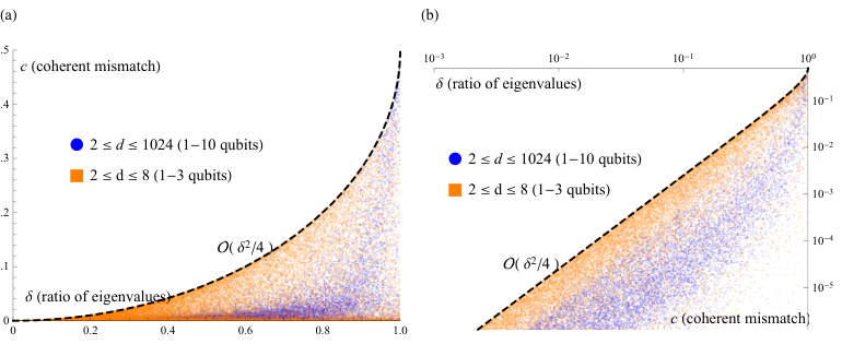
Fig. 3 shows the coherent mismatch in case of randomly generated quantum states. Orange rectangles (blue dots) in Fig. 3 correspond to quantum states whose dimension was generated uniformly randomly in the range (). Indeed, saturating the upper bound (dashed black line) is significantly less likely in larger dimensions (blue rectangles are significantly below upper bound). This is expected since the extremal quantum states occupy a rapidly decreasing portion of the full volume of state space. Refer to Appendix L for more details.
III.1.4 Limiting scenarios
We have found in the previous section that the error states that saturate the error bound depend on the parameter which quantifies the ratio of the eigenvalues (ideal state vs. dominant eigenvalue of the error state , see Definition 1).
In the limiting scenario when the contribution of the error density matrix is much smaller than the ideal state we obtain the limit . In this limit the dominant eigenvector of the extremal error state is an equal superposition
| (10) |
due to Theorem 1 where is an arbitrary error state that is orthogonal to . This also informs us that the extremal quantum states in the practically relevant regime (i.e., for small ) have dominant error vectors of the form, i.e., .
On the other hand, when the contribution of the error state is as strong as the ideal state via then the worst-case error vector is almost orthogonal to the ideal state via some small
Surprisingly, we find that the global worst-case error, i.e., when , can only be saturated by the quantum state in the limit when (one must compute the limit only after computing ) as
To illustrate this, in the second equation above we have computed the matrix representation of the quantum state in the -dimensional subspace spanned by the orthonormal vectors and to leading order in . Indeed, the dominant eigenvector of this density matrix is the vector (up to an error ) and this vector has a fidelity to the ideal computational state . The limit of the coherent mismatch is thus well-defined, however, note that the state itself in the limit becomes trivially the identity matrix (commuting case).
Interestingly, here we find exactly the opposite behaviour when compared to the case of eigenvalues in Weyl’s inequalities in Sec. II.2. Recall that for the sum of two matrices the extremal shift to the eigenvalues (Weyl inequalities) is saturated when the dominant eigenvector of is actually . In stark contrast, we have found above that the extremal coherent mismatch (extremal shift in the dominant eigenvector) is saturated only in the limit when the dominant eigenvector of is orthogonal to .
III.1.5 Application to error suppression
Let us finally remark on the implications of the above results to the performance of the ESD and VD approach. Recall that ref. Koczor 2021 established general scaling results on how many copies are required to reach a precision in suppressing the noise when measuring expectation values in the dominant eigenvector.
Let us now assume that the aim is to suppress this error level to the level of error caused by the coherent mismatch (assuming normalised observables ). Consistent with Theorem 1, we assume that the quantum state and the noise is of the form of Eq. (4) as and assume that the quantum states are considerably noisy with being sufficiently large as relevant in practice, i.e., in general and when we aim to prepare eigenstates. These two conditions correspond to circuit error rates and , respectively, which is reasonable to assume in practice. If we set our target precision to be the general trace distance bound from Sec. II.1 as , then we obtain the following result in Appendix G: we find that we need at least copies to reach the target precision with the worst-case extremal states. Interestingly, ref. Czarnik et al. 2021 found in numerical simulations of noisy derangement circuits that, for the considered circuits, at least copies were required to reach a noise floor determined by the coherent mismatch and by the noise in the controlled-SWAP operations.
On the other hand, if our aim is to prepare eigenstates as discussed in Sec. II.1, then the coherent mismatch is guaranteed to cause a quadratically smaller error. We thus set the target precision to and find in Appendix G that we need at least copies to reach the noise floor in the practically relevant region where states are considerably noisy (via circuit error rates ). This confirms prior numerical simulations (Fig. 4 in ref. Koczor 2021).
While we have derived these results for the extremal quantum states, it stands to reason that in more realistic scenarios one may need significantly more copies to reach the precision as limited by the coherent mismatch. Furthermore, these arguments establish that as long as the quantum device is limited to preparing only a small number of copies (e.g., , or depending on hardware constraints) of the noisy quantum state, then the error introduced by the coherent mismatch will be guaranteed to be smaller than the error caused by having too few copies (not sufficient suppression).
III.2 Lower and upper bounds via commutators
While the previously derived bounds are tight as they are saturated by the extremal states, they can be generally very pessimistic since the extremal states are very unlikely to be relevant in practice. This is nicely illustrated in Fig. 3 where most randomly generated quantum states are significantly below this bound (dashed black lines) especially as the dimensionality grows (orange vs. blue). In fact, the previous bound can be arbitrarily pessimistic, since generally there is no lower bound of in terms of : when is non-zero then can still be zero when and commute. This leads to our next point: to derive general upper and lower bounds in terms of the commutator. These bounds will in turn be independent of the non-unique decomposition in Eq. (4) and will also allow us to derive scaling results due to the asymptotically coinciding lower and upper bounds.
III.2.1 Expressing the commutator norm
As we discussed above, if the error matrix commutes with the ideal state than the coherent mismatch must vanish. Similarly we would expect that if the commutator is ‘large’ than the coherent mismatch should also be large. In the following we would like to introduce a measure of how large the commutator is. For this purpose we will use a suitable matrix norm which we will aim to upper bound.
Interestingly, it has been an open problem in mathematics to upper bound the Hilbert-Schmidt or Frobenius norm of the commutator between two matrices and was only very recently solved for general matrices, refer to refs. Böttcher and Wenzel 2008; Vong and Jin 2008; Wu and Liu 2010; Böttcher and Wenzel 2005; László 2007; Cheng et al. 2010; Wenzel and Audenaert 2010 for more details. In particular, it was found that the norm of the commutator of two generic matrices is upper bounded as
| (11) |
As opposed to generic matrices, in the present case we aim to express the norm of the commutator of two density matrices . Although we make no assumption about (except that it is a density matrix), is a special matrix, i.e., a projector, since it represents a pure quantum state. This property allows us to express the commutator norm more explicitly.
Statement 3.
We analytically solve the eigenvalues and eigenvectors of both the matrix from Statement 1 and the commutator . We establish that both matrices have only two non-zero eigenvalues as and . It follows that their matrix norms are equivalent
for all . The eigenvalue can be computed as
which expresses a generalised variance of the density matrix and is the fidelity.
Refer to Appendix H for a proof. Interestingly, we can directly relate the off-diagonal entries of the arrowhead matrix—as determined by —from Statement 1 to the commutator . Furthermore, the above result establishes that the commutator norm is exactly given by a generalised uncertainty which is a notion widely used in quantum theory to express the variance of measurement statistics of an observable in, e.g., quantum metrology Pezzè et al. 2018 and beyond Sakurai 1994. In the present case the observable is the operator and the state is the ideal computational state . It is also interesting to note that this commutator norm is proportional to the quantum Fisher information Liu et al. 2019 of the quantum state in a unitary parametrisation generated by the Hamiltonian .
Let us now illustrate how using the above expressions yield improved bounds when compared to the general bounds considered in the literature. As such, it is straightforward to show that
and this bound is indeed considerably tighter than the prior general result in Eq. 11 since for states of low purity (i.e., ) we find that . Furthermore, assuming the decomposition from Eq. (4) we obtain the general bound , where was defined in Definition 1 and was the extremal shift in the Weyl inequalities in Remark 1.
III.2.2 Upper bound via commutator norm
We are now prepared to derive a general upper bound of the coherent mismatch based on the previously obtained norms of the commutator.
Theorem 2.
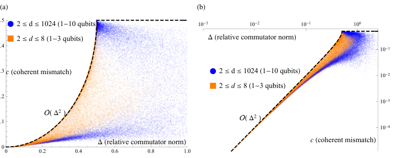
Let us define the metric that depends only on two parameters: the relative commutator norm , where the commutator norm was defined in Statement 3 and the ratio of the two dominant eigenvalues is . For any fixed there exist an infinite number of worst-case scenario states that saturate the upper bound of the coherent mismatch as
| (12) |
These extremal states have eigenvectors that are orthogonal to the ideal state , except for the two dominant eigenvectors that correspond to the two dominant eigenvalues .
The above upper bound is saturated by extremal states similar to the ones in Theorem 1. The crucial difference, however, is that this upper bound is completely independent of the (not necessarily unique) decomposition into an ideal and noisy quantum states from Eq. (4). The present bound can thus be applied to more general scenarios too (note that the definition of the extremal states above is independent of ).
Fig. 4 shows the coherent mismatch as a function of the metric for randomly generated density matrices in various dimensions (blue dots and orange rectangles). The upper bound (dashed black lines) is significantly more likely to be saturated by random states in lower dimensions (orange rectangles) since the extremal states occupy a negligible volume of the increasingly higher dimensional state space. We can identify two distinct regions in the plots.
First, for large most of the randomly generated states are significantly below the bound, similarly as in Fig. 3. Note also that the metric can in principle be larger than and in such a scenario Eq. (12) is not defined. For this reason Fig. 4 shows the general bound in this region. We note, however, that this region is not relevant in practice since typical quantum circuits in near-term quantum devices produce errors that typically result in relatively small commutator norms as discussed in Sec. IV.
Second, in the practically more relevant region where is sufficiently small, one can observe that all the randomly generated states nearly saturate the upper bound. The reason for this behaviour will be clarified in the next section where we derive a general lower bound on and show that it approaches the upper bound as decreases – thus tightly confining the possible values that can take up. Let us now introduce this lower bound.
III.2.3 Lower bound via commutator norm and application to error suppression
Using the same technique as in Theorem 2 we can derive a directly analogous lower bound for the coherent mismatch.
Lemma 1.
Let us define the metric that depends only on two parameters: the relative commutator norm and the ratio where is the smallest non-zero eigenvalue of . For any fixed there exist an infinite number of best-case scenario states that saturate the lower bound of the coherent mismatch as
| (13) |
The dominant eigenvector of the extremal state and its eigenvector that corresponds to the smallest non-zero eigenvalue have non-zero overlaps with the ideal computational state . All other eigenvectors of with are orthogonal to the the ideal state .
Refer to Appendix J for a proof. The above Lemma guarantees that the coherent mismatch is always at least as large as the above lower bound for a fixed . Note that the upper bounds in Theorem 2 are similarly determined by : the most important consequence is that for a sufficiently small coherent mismatch , the possible values that can take up are tightly confined by the upper and lower bounds. This is illustrated in Fig. 4: all randomly generated states with small nearly saturate the upper bound.
To substantiate this observation let us compute the ratio of the lower and upper bounds as
| (14) |
Let us now consider 3 different scenarios in which the above ratio approaches and thus the lower and upper bounds coincide.
First, the ratio approaches when the suppression factor is very small . Such a small suppression factor guarantees high efficacy of the ESD/VD approach as established in ref. Koczor 2021, but it may not be reasonable to expect vanishingly small suppression factors for realistic noisy circuits with a large number of gates, refer to Sec. IV. On the other hand, even a realistic would result in approximately a factor of ratio between the lower and upper bounds which is already reasonably tight.
Second, the approximation in Eq. 14 depends on the difference between the largest and smallest ‘error’ probabilities (eigenvalues of from Eq. (2)). Indeed, need not vanish in order for the ratio in Eq. (14) to approach : it is sufficient that the smallest and largest ‘error’ probabilities are close via . This is naturally the case for the extremal, rank- error states from Sec. III.1.4 for which and we are thus guaranteed that the bounds coincide and are simultaneously saturated.
Third, one can generally expect that the above difference between the largest and smallest error probabilities is determined by the entropy of the error probability distributions. In particular, ref. Koczor 2021 introduced the error probability vector and established that the efficacy of the ESD/VD approach depends on the Rényi entropies of this probability vector. Indeed the difference generally decays exponentially with the entropy and regardless of the value of the difference of the eigenvalues is negligibly small for high-entropy probability distributions. One can thus generally expect that for high-entropy experimental states the possible values of the coherent mismatch are tightly confined by the lower and upper bounds.
IV Application to quantum circuits
IV.1 Approximating commutators in noisy quantum circuits
Let us now consider noisy quantum circuits that prepare quantum states via mappings as discussed in Sec. I.1. Since the commutator norm has a special significance (see Sec. III.2) our aim in the following is to approximate the commutator norm for these quantum circuits.
First, let us consider the limiting global worst-case scenario in which case the ideal unitary computation is followed by a global error channel with probability as . This is a special case of Eq. 1 in which all gates are perfect, except for the last one. The commutator norm in this case is generally upper bounded as and the bound is saturated when the mapping prepares the extremal states in Eq. (III.1.4).
Let us now consider the error channel from Eq. 1 and assume that every gate has an identical error probability . Let us now make another simplification for ease of notation and focus on the case when for all : such as in case of dephasing noise. While these assumptions greatly simplify the following derivations we remark that the present results can be generalised straightforwardly as discussed in Appendix K.2.
The considered error model maps the density matrix to an incoherent superposition (mixture) of (where is the number of gates) pure states which correspond to individual error events. For example, the pure state represents the event where an error happens during the execution of the gate but all other gates are noiseless – this occurs with probability , refer to Appendix K for more details. In general we find that there are overall different events where errors happen and each of these have probabilities .
As such, we can approximate from Eq. 4 via the probability that no error happens as
| (15) |
where we have introduced the usual circuit error rate to denote the expected number of errors in the full circuit. Indeed, for a sufficiently large number of gates the probability that no error happens decays exponentially with .
We compute the norm (from Statement 3) of the commutator in Appendix K assuming the above error model and obtain the expression
| (16) |
Here the index set indexes all distinct error events and there are exponentially many of them. Here, are probabilities of the individual error events, while are real numbers that depend on the scalar products between the different erroneous states and are thus generally upper bounded as .
The diagonal terms in the above sum are strictly non-negative and we can obtain a general upper bound by analytically evaluating the summation as
| (17) |

In contrast, the off-diagonal terms in the summation in Eq. (16) depend on the relative phase between the state vectors of the erroneous quantum states. We can generally upper bound the summation in Eq. (16) and obtain the completely general upper bound which is approximated by for small error rates. This bound is indeed pessimistic: even the global worst-case scenario discussed above has a guaranteed bound which is by a factor of smaller.
In order to be able to establish a more meaningful upper bound, we now consider a rather artificial assumption: we assume that the off-diagonal terms with in Eq. (16) are random variables with mean and some variance . This is equivalent to assuming that complex phases (relative to the ideal state ) of the erroneous pure states uniformly cover the complex plane. We stress that this assumption is not equivalent to non-entangling random circuits undergoing single-qubit depolarising noise considered in ref. Huggins et al. 2020. Those circuits map to noise that commutes with the ideal state and indeed one trivially finds that . In contrast, ref. Huggins et al. 2020 demonstrated that relatively deep entangling random circuits result in a coherent mismatch that is non-zero and comparable to that of non-random circuits.
The above point can be illustrated via the following analogy: suppose that we sum up random real numbers (drawn from a distribution of mean and variance ). The sum of these numbers is highly unlikely to be . In fact, the result is another random number that is upper bounded with high probability by some multiple of the square-root of the total variance that we can compute as . In analogy to this observation, we compute the total variance in Appendix K and approximately upper bound the summation from Eq. (16) as
| (18) |
where was defined in Eq. (17) as the general upper bound on the diagonal entries. Interestingly, we thus find that assuming randomly distributed off-diagonal entries, the total sum is only by a constant multiplicative factor larger than the upper bound of the diagonal entries. Let us now analyse this upper bound.
IV.2 Analysing the approximate bound
Let us now analyse in detail the upper bound function from Eqs. (17)-(18). In particular, in Appendix K.1 we obtain the approximation
| (19) |
up to a negligible multiplicative error (that vanishes for large ) that we neglect for ease of notation. This approximation is plotted in Fig. 5 as a function of the circuit error rate . In the plot one can recognise the following 3 distinct regions.
(a) When the circuit error rate is small we find that the upper bound increases in quadratic order as . We can compare this expression to the global worst-case scenario scaling and deduce that the present bound decreases inversely proportionally with the number of gates (at a fixed error rate ). This is illustrated in Fig. 5 where the function (solid black lines) are indeed significantly below the global worst-case bound (dashed black lines), approximately by a factor up to the constant factor from Eq. (18).
(b) The maximum of the function is at
| (20) |
and this position is independent of the constant multiplicative factor from Eq. (18). It is also interesting to note that the global maximum of the function is
proportional to . This informs us that the maximum of the bound is decreased inversely proportionally when increasing the number of gates similarly to (a). In fact, one can generally state that the upper bound in Eq. (18) scales as for any fixed .
(c) The function starts to decrease in the third region where and decreases in exponential order asymptomatically for . On the other hand, we observe that in the region where , our approximation breaks down: in some instances we numerically observe a different scaling in this regime, especially when the circuits are highly deterministic. We have performed additional simulations to illustrate this point: in Fig. 7 the commutator norm decreases more slowly for highly deterministic circuits (constant rotation angles in the quantum gates) in the region . Nevertheless, this region is not particularly relevant in practice for the following reason. In the context of the ESD/VD approach the number of circuit repetitions required to suppress shot noise scales exponentially with the circuit error rate via Eq. (15). It in fact generally holds for error mitigation techniques that their costs grow exponentially and one thus needs to guarantee a bounded . For example, assuming a quadratic (standard shot noise) scaling of the measurement costs, the overhead at is approximately a factor of which is certainly prohibitive in practice Koczor 2021; van Straaten and Koczor 2021.
On the other hand, we remarkably find that our bounds hold surprisingly well in all scenarios in the practically most important region when . In particular, these bounds seem to hold remarkably well even for highly deterministic circuits in Fig. 7, such as circuits with constant rotation angles – despite that we assumed randomly distributed phases for our approximate bounds. Furthermore, even error models that are beyond the scope of Eq. (1), such as damping in Fig. 5, seem to result in exactly the same kind of scaling. The numerical data seem to be independent of the number of qubits too (compare blue, red and black in Fig. 5 and in Fig. 7) as long as the number of gates is fixed, which is consistent with the theoretical bounds. Most remarkably, up until the point each of the large variety of circuits simulated in this work resulted in exactly the same type of scaling with respect to and up to only a small (relative to ) global multiplication factor.
These observations are supported in Appendix K.2 where extensions of our bound to more general error models are discussed: the form of the upper bound function in Eq. (18) is expected to be the same even if one allows higher rank Kraus maps as in Eq. (1) or when one allows different error probabilities for different gates via . Interestingly, if a fraction of the gates commutes with the error Kraus maps then our bound function still holds up to a minor re-scaling of its argument (via a multiplication with a constant). Let us now apply our results to bounding the coherent mismatch.
IV.3 Application to coherent mismatch and noise floor
Let us now consider the upper bound for the coherent mismatch via Theorem 2 that depends on the commutator norm. Let us assume that the commutator norm is bounded via Eq. (18) and we then obtain
| (21) |
where we have used that the probability of the ideal state is upper bounded as via Eq. (15). Let us now remark on 3 important consequences of the above approximate bound and how it confirms prior numerical observations.
(a) Eq. (21) establishes that the coherent mismatch scales as when assuming a fixed , where was defined in Theorem 2 as the ratio of the two largest eigenvalues. This scaling is consistent with previous numerical observations: It was numerically observed in ref. Koczor 2021 (ref. Huggins et al. 2020) that if one increases the per-gate error probability in a fixed quantum circuit then the coherent mismatch (noise floor) grows quadratically (linearly) as ().
(b) Eq. (21) establishes a scaling when increasing the number of gates at a fixed per-gate error rate. This is consistent with the observation of ref. Koczor 2021 that increasing the number of gates in a circuit of fixed per-gate error probability increases the coherent mismatch proportionally as , while ref. Huggins et al. 2020 similarly observed in numerical random-circuit simulations that the noise floor slightly increases when increasing . As noted in the above section, the scaling results in this work were derived assuming sufficiently complex quantum circuits, but these results appear to hold remarkably well for even highly deterministic circuits too as long as the circuit error rate does not significantly exceed .
The crucial implication of this scaling for practical applications is the following. Consider a computational task that is defined for qubits. A quantum circuit of depth then requires overall gates to implement the computation. This ensures us that the coherent mismatch decreases even for constant depth as when the size of the computation (via ) is increased at a constant circuit error rate . In practice one needs to keep at least bounded to ensure a bounded sampling cost which was discussed in the previous section.
(c) Another important consequence of these scaling results is the following. Recall that the probability that no error happens decays exponentially with the circuit error rate as . This is approximately constant for a fixed value of . In stark contrast, we have found that the coherent mismatch depends on the number of gates and scales as . Let us now compare the fidelity that decreases due to incoherent errors and the coherent fidelity that decreases due to the coherent mismatch in the dominant eigenvector. The fidelity can be approximated as and decays exponentially due to incoherent errors, while the fidelity due to the coherent mismatch decays as . The ratio of these two fidelities can then be approximated as
Indeed the above ratio increases exponentially when increasing within a finite range, e.g., when and when the number of gates is sufficiently large. This is consistent with numerical observations of ref. Koczor 2021: increasing the number of gates in a sufficiently complex circuit decreases the incoherent fidelity () exponentially faster than it decreases the coherent fidelity (). Very importantly, this ensures us that the coherent mismatch of the dominant eigenvector (which cannot be suppressed) causes an exponentially smaller error when compared to the incoherent decay of the fidelity . Here the latter can indeed be suppressed exponentially by increasing the number of copies in the ESD/VD approach.
V Discussion and Conclusion
The present work considered the fundamental question: given a noisy quantum state, how well does its dominant eigenvector approximate a corresponding ideal, noise-free computation ? While it is of fundamental importance to understand how noise affects quantum systems, this particular question has crucial practical relevance. The recently introduced ESD/VD error suppression techniques are ultimately limited by the coherent mismatch.
This work has established general upper bounds and scaling results for the coherent mismatch and presented a comprehensive analysis of its implications in practically relevant scenarios. As such, it was established that the coherent mismatch is indeed negligibly small for sufficiently complex noisy quantum circuits, typically used in variational quantum algorithms and other near-term quantum algorithms Endo et al. 2020; Cerezo et al. 2020; Bharti et al. 2021. It is interesting to note that since variational quantum algorithms rely on optimising a cost function, this optimisation can be expected to anyway minimise the effect of the coherent mismatch. Let us briefly summarise the most important results.
(a) The bound based on the noise floor in ref. Huggins et al. 2020 was improved and quadratically smaller bounds are obtained for the pivotal case of preparing eigenstates – see Sec. II.1.
(b) A general upper bound for the coherent mismatch was obtained in Sec. III.1.3 by explicitly constructing worst-case scenario extremal quantum states that saturate it (for this we analytically computed the coherent mismatch in Sec. III.1.2 using our arrowhead decomposition obtained in Sec. III.1.1). The present problem is closely related to an important problem in mathematics: bounding the eigenvalues of a sum of two matrices (Weyl inequalities). While those bounds are well-known to be saturated by identical dominant eigenvectors, it was shown in Sec. III.1.4 that bounds obtained in this work are in stark contrast saturated by the close-to-orthogonal dominant eigenvectors of the extremal quantum states.
(c) In the ESD/VD approach, even for extremal quantum states, one needs at least copies of the noisy state to suppress errors to the noise floor set by the coherent mismatch, see Sec. III.1.5. The coherent mismatch is thus guaranteed to be negligible in practical applications where the quantum device is limited in its ability to prepare a large number of copies.
(d) Another closely related problem in mathematics is upper bounding the matrix norm of the commutator of two matrices. We obtained considerably tighter bounds then prior results in the specific case of the matrix norm of the commutator between two density matrices, see Sec. III.2.1. Interestingly, the commutator norm is given by the generalised quantum-mechanical variance of the density matrix which quantity is also proportional to the quantum Fisher information.
(e) General upper and lower bounds were obtained in Sec. III.2.2 and Sec. III.2.3 for the coherent mismatch in terms of the commutator norm from (d). It was established that in the practically important region the upper and lower bounds are close to each other and thus tightly confine possible values of – while the bounds asymptomatically coincide. It was also shown that the coherent mismatch generally decays exponentially with Rényi entropies of the error probabilities – indeed, similar scaling results were obtained in ref. Koczor 2021 for the efficacy of the ESD/VD approach and it was noted that near-term quantum devices are expected to produce high-entropy errors.
(f) We finally applied the above general results to the specific but pivotal case of noisy quantum circuits in Sec. IV. The resulting approximate bounds confirmed scaling results of ref. Koczor 2021: the coherent mismatch in sufficiently complex noisy circuits is decreased inversely proportionally when increasing the size of the computation (by increasing the number of qubits at a fixed error rate). Furthermore, in the practically important regions, the incoherent deterioration of a quantum state is exponentially more severe than the drift in the dominant eigenvector. This establishes that the coherent mismatch is indeed negligible in relevant applications of the ESD/VD approach.
Results obtained in this work pave the way towards developing advanced error mitigation techniques that will be crucial for the successful exploitation of noisy quantum devices. A number of apparent questions will be worth investigating in the future, such as developing twirling techniques (and generalisations thereof) that potentially decrease the coherent mismatch without affecting the ideal part of the computation. In particular, one could obtain a series of quantum circuits whose unitary component is identical for every while the noise component is different. The average of such channels is thus guaranteed to increase the entropy of errors resulting in a smaller coherent mismatch.
Another open question is related to similar themes in mathematics: Analogously to the Weyl inequalities for the eigenvalues, is it possible to generalise the present results to obtain a series of upper and lower bounds for infidelities in all eigenvectors (not just the dominant one)? Answering this question will be highly non-trivial since the generalisation to arbitrary matrices will require to go beyond the analytical expressions obtained for and which assumed that is rank-1 thus having only a single dominant component.
Let us finally remark that arguments presented in this work naturally generalise to infinite-dimensional quantum states as general trace-class operators.
Acknowledgments
I would like to thank Simon C. Benjamin, Earl Campbell and Sam McArdle for useful discussions. I would like to thank Robert Zeier, Zhenyu Cai and Adrian Chapman for their valuable comments and for carefully reading drafts of this work. I acknowledge funding received from EU H2020-FETFLAG-03-2018 under the grant agreement No 820495 (AQTION) and from EPSRC Hub grant under the agreement number EP/T001062/1. I acknowledge financial support from the Glasstone Research Fellowship of the University of Oxford. The numerical modelling involved in this study made use of the Quantum Exact Simulation Toolkit (QuEST), and the recent development QuESTlink Jones and Benjamin 2020 which permits the user to use Mathematica as the integrated front end. I am grateful to those who have contributed to both these valuable tools.
References
- Arute et al. (2019) F. Arute, K. Arya, R. Babbush, and et al., Quantum supremacy using a programmable superconducting processor, Nature 574, 505 (2019).
- Zhong et al. (2020) H.-S. Zhong, H. Wang, Y.-H. Deng, M.-C. Chen, L.-C. Peng, Y.-H. Luo, J. Qin, D. Wu, X. Ding, Y. Hu, P. Hu, X.-Y. Yang, W.-J. Zhang, H. Li, Y. Li, X. Jiang, L. Gan, G. Yang, L. You, Z. Wang, L. Li, N.-L. Liu, C.-Y. Lu, and J.-W. Pan, Quantum computational advantage using photons, Science 370, 1460 (2020), https://science.sciencemag.org/content/370/6523/1460.full.pdf .
- McArdle et al. (2020) S. McArdle, S. Endo, A. Aspuru-Guzik, S. C. Benjamin, and X. Yuan, Quantum computational chemistry, Rev. Mod. Phys. 92, 015003 (2020).
- Preskill (2018) J. Preskill, Quantum Computing in the NISQ era and beyond, arXiv preprint arXiv:1801.00862 (2018).
- Farhi et al. (2014) E. Farhi, J. Goldstone, and S. Gutmann, A quantum approximate optimization algorithm, arXiv preprint arXiv:1411.4028 (2014).
- Peruzzo et al. (2014) A. Peruzzo, J. McClean, P. Shadbolt, M.-H. Yung, Q. Zhou, P. J. Love, A. Aspuru-Guzik, and J. L. O’Brien, A variational eigenvalue solver on a photonic quantum processor, Nature communications 5 (2014).
- O’Malley et al. (2016) P. J. J. O’Malley, R. Babbush, I. D. Kivlichan, J. Romero, J. R. McClean, R. Barends, J. Kelly, P. Roushan, A. Tranter, N. Ding, B. Campbell, Y. Chen, Z. Chen, B. Chiaro, A. Dunsworth, A. G. Fowler, E. Jeffrey, E. Lucero, A. Megrant, J. Y. Mutus, M. Neeley, C. Neill, C. Quintana, D. Sank, A. Vainsencher, J. Wenner, T. C. White, P. V. Coveney, P. J. Love, H. Neven, A. Aspuru-Guzik, and J. M. Martinis, Scalable Quantum Simulation of Molecular Energies, Phys. Rev. X 6, 031007 (2016).
- McClean et al. (2016) J. R. McClean, J. Romero, R. Babbush, and A. Aspuru-Guzik, The theory of variational hybrid quantum-classical algorithms, New J. Phys. 18, 023023 (2016).
- Paesani et al. (2017) S. Paesani, A. A. Gentile, R. Santagati, J. Wang, N. Wiebe, D. P. Tew, J. L. O’Brien, and M. G. Thompson, Experimental Bayesian Quantum Phase Estimation on a Silicon Photonic Chip, Phys. Rev. Lett. 118, 100503 (2017).
- Li and Benjamin (2017) Y. Li and S. C. Benjamin, Efficient Variational Quantum Simulator Incorporating Active Error Minimization, Phys. Rev. X 7, 021050 (2017).
- Colless et al. (2018) J. I. Colless, V. V. Ramasesh, D. Dahlen, M. S. Blok, M. E. Kimchi-Schwartz, J. R. McClean, J. Carter, W. A. de Jong, and I. Siddiqi, Computation of Molecular Spectra on a Quantum Processor with an Error-Resilient Algorithm, Phys. Rev. X 8, 011021 (2018).
- Santagati et al. (2018) R. Santagati, J. Wang, A. A. Gentile, S. Paesani, N. Wiebe, J. R. McClean, S. Morley-Short, P. J. Shadbolt, D. Bonneau, J. W. Silverstone, D. P. Tew, X. Zhou, J. L. O’Brien, and M. G. Thompson, Witnessing eigenstates for quantum simulation of Hamiltonian spectra, Science Advances 4, 10.1126/sciadv.aap9646 (2018).
- Kandala et al. (2017) A. Kandala, A. Mezzacapo, K. Temme, M. Takita, M. Brink, J. M. Chow, and J. M. Gambetta, Hardware-efficient variational quantum eigensolver for small molecules and quantum magnets, Nature 549, 242 (2017).
- Kandala et al. (2019) A. Kandala, K. Temme, A. D. Córcoles, A. Mezzacapo, J. M. Chow, and J. M. Gambetta, Error mitigation extends the computational reach of a noisy quantum processor, Nature 567, 491 (2019).
- Hempel et al. (2018) C. Hempel, C. Maier, J. Romero, J. McClean, T. Monz, H. Shen, P. Jurcevic, B. P. Lanyon, P. Love, R. Babbush, A. Aspuru-Guzik, R. Blatt, and C. F. Roos, Quantum Chemistry Calculations on a Trapped-Ion Quantum Simulator, Phys. Rev. X 8, 031022 (2018).
- Kokail et al. (2019) C. Kokail, C. Maier, R. van Bijnen, T. Brydges, M. K. Joshi, P. Jurcevic, C. A. Muschik, P. Silvi, R. Blatt, C. F. Roos, et al., Self-verifying variational quantum simulation of lattice models, Nature 569, 355 (2019).
- Koczor et al. (2020) B. Koczor, S. Endo, T. Jones, Y. Matsuzaki, and S. C. Benjamin, Variational-State Quantum Metrology, New J. Phys. 22, 083038 (2020).
- Koczor and Benjamin (2019) B. Koczor and S. C. Benjamin, Quantum natural gradient generalised to non-unitary circuits, arXiv preprint arXiv:1912.08660 (2019).
- Koczor and Benjamin (2020) B. Koczor and S. C. Benjamin, Quantum analytic descent, arXiv preprint arXiv:2008.13774 (2020).
- Endo et al. (2020) S. Endo, Z. Cai, S. C. Benjamin, and X. Yuan, Hybrid quantum-classical algorithms and quantum error mitigation, arXiv preprint arXiv:2011.01382 (2020).
- Cerezo et al. (2020) M. Cerezo, A. Arrasmith, R. Babbush, S. C. Benjamin, S. Endo, K. Fujii, J. R. McClean, K. Mitarai, X. Yuan, L. Cincio, et al., Variational quantum algorithms, arXiv preprint arXiv:2012.09265 (2020).
- Bharti et al. (2021) K. Bharti, A. Cervera-Lierta, T. H. Kyaw, T. Haug, S. Alperin-Lea, A. Anand, M. Degroote, H. Heimonen, J. S. Kottmann, T. Menke, et al., Noisy intermediate-scale quantum (NISQ) algorithms, arXiv preprint arXiv:2101.08448 (2021).
- Koczor (2021) B. Koczor, Exponential error suppression for near-term quantum devices, Phys. Rev. X 11, 031057 (2021).
- Huggins et al. (2020) W. J. Huggins, S. McArdle, T. E. O’Brien, J. Lee, N. C. Rubin, S. Boixo, K. B. Whaley, R. Babbush, and J. R. McClean, Virtual distillation for quantum error mitigation, arXiv preprint arXiv:2011.07064 (2020).
- Böttcher and Wenzel (2008) A. Böttcher and D. Wenzel, The Frobenius norm and the commutator, Linear algebra and its applications 429, 1864 (2008).
- Vong and Jin (2008) S.-W. Vong and X.-Q. Jin, Proof of Bottcher and Wenzel’s Conjecture, Oper. Matrices 2, 435 (2008).
- Wu and Liu (2010) Y.-D. Wu and X.-Q. Liu, A short note on the Frobenius norm of the commutator, Mathematical Notes 87, 903 (2010).
- Böttcher and Wenzel (2005) A. Böttcher and D. Wenzel, How big can the commutator of two matrices be and how big is it typically?, Linear algebra and its applications 403, 216 (2005).
- László (2007) L. László, Proof of Böttcher and Wenzel’s conjecture on commutator norms for 3-by-3 matrices, Linear algebra and its applications 422, 659 (2007).
- Cheng et al. (2010) C.-M. Cheng, S.-W. Vong, and D. Wenzel, Commutators with maximal Frobenius norm, Linear algebra and its applications 432, 292 (2010).
- Wenzel and Audenaert (2010) D. Wenzel and K. M. Audenaert, Impressions of convexity: an illustration for commutator bounds, Linear algebra and its applications 433, 1726 (2010).
- Nielsen and Chuang (2011) M. A. Nielsen and I. L. Chuang, Quantum Computation and Quantum Information, 10th ed. (Cambridge University Press, New York, NY, USA, 2011).
- Czarnik et al. (2021) P. Czarnik, A. Arrasmith, L. Cincio, and P. J. Coles, Qubit-efficient exponential suppression of errors, arXiv preprint arXiv:2102.06056 (2021).
- Weyl (1912) H. Weyl, Das asymptotische Verteilungsgesetz der Eigenwerte linearer partieller Differentialgleichungen (mit einer Anwendung auf die Theorie der Hohlraumstrahlung), Math. Ann. 71, 441 (1912).
- Klyachko (1998) A. A. Klyachko, Stable bundles, representation theory and Hermitian operators, Selecta Mathematica, New Series 4, 419 (1998).
- Helmke and Rosenthal (1995) U. Helmke and J. Rosenthal, Eigenvalue inequalities and Schubert calculus, Mathematische Nachrichten 171, 207 (1995).
- Knutson and Tao (1999) A. Knutson and T. Tao, The honeycomb model of GLn tensor products I: Proof of the saturation conjecture, Journal of the American Mathematical Society 12, 1055 (1999).
- Knutson et al. (2004) A. Knutson, T. Tao, and C. Woodward, The honeycomb model of GLn tensor products II: Puzzles determine facets of the Littlewood-Richardson cone, Journal of the American Mathematical Society 17, 19 (2004).
- Knutson and Tao (2001) A. Knutson and T. Tao, Honeycombs and sums of Hermitian matrices, Notices Amer. Math. Soc 48 (2001).
- Gu and Eisenstat (1995) M. Gu and S. C. Eisenstat, A divide-and-conquer algorithm for the symmetric tridiagonal eigenproblem, SIAM Journal on Matrix Analysis and Applications 16, 172 (1995).
- Bixon and Jortner (1968) M. Bixon and J. Jortner, Intramolecular radiationless transitions, The Journal of chemical physics 48, 715 (1968).
- Gadzuk (1981) J. Gadzuk, Localized vibrational modes in Fermi liquids. General theory, Physical Review B 24, 1651 (1981).
- O’leary and Stewart (1990) D. O’leary and G. Stewart, Computing the eigenvalues and eigenvectors of symmetric arrowhead matrices, Journal of Computational Physics 90, 497 (1990).
- Sakurai (1994) J. J. Sakurai, Modern Quantum Mechanics, rev. ed. (Addison-Wesley, Reading, 1994).
- Wilkinson (1965) J. H. Wilkinson, The algebraic eigenvalue problem, Vol. 87 (Clarendon press Oxford, 1965).
- Ekert et al. (2002) A. K. Ekert, C. M. Alves, D. K. Oi, M. Horodecki, P. Horodecki, and L. C. Kwek, Direct estimations of linear and nonlinear functionals of a quantum state, Phys. Rev. Lett. 88, 217901 (2002).
- Keyl and Werner (2001) M. Keyl and R. F. Werner, Estimating the spectrum of a density operator, Phys. Rev. A 64, 052311 (2001).
- Marvian and Spekkens (2014) I. Marvian and R. W. Spekkens, A generalization of Schur–Weyl duality with applications in quantum estimation, Communications in Mathematical Physics 331, 431 (2014).
- Acharya et al. (2020) J. Acharya, I. Issa, N. V. Shende, and A. B. Wagner, Estimating Quantum Entropy, IEEE Journal on Selected Areas in Information Theory 1, 454 (2020).
- Tanaka et al. (2014) T. Tanaka, Y. Ota, M. Kanazawa, G. Kimura, H. Nakazato, and F. Nori, Determining eigenvalues of a density matrix with minimal information in a single experimental setting, Phys. Rev. A 89, 012117 (2014).
- Christandl et al. (2007) M. Christandl, A. W. Harrow, and G. Mitchison, Nonzero Kronecker coefficients and what they tell us about spectra, Comm. Math. Phys. 270, 575 (2007).
- Christandl and Mitchison (2006) M. Christandl and G. Mitchison, The spectra of quantum states and the Kronecker coefficients of the symmetric group, Communications in mathematical physics 261, 789 (2006).
- Pezzè et al. (2018) L. Pezzè, A. Smerzi, M. K. Oberthaler, R. Schmied, and P. Treutlein, Quantum metrology with nonclassical states of atomic ensembles, Rev. Mod. Phys. 90, 035005 (2018).
- Liu et al. (2019) J. Liu, H. Yuan, X.-M. Lu, and X. Wang, Quantum Fisher information matrix and multiparameter estimation, Journal of Physics A: Mathematical and Theoretical (2019).
- van Straaten and Koczor (2021) B. van Straaten and B. Koczor, Measurement Cost of Metric-Aware Variational Quantum Algorithms, PRX Quantum 2, 030324 (2021).
- Jones and Benjamin (2020) T. Jones and S. Benjamin, Questlink—mathematica embiggened by a hardware-optimised quantum emulator, Quantum Sci. Techn. 5, 034012 (2020).
- Cai (2020) Z. Cai, Multi-exponential error extrapolation and combining error mitigation techniques for nisq applications, arXiv preprint arXiv:2007.01265 (2020).
Appendix A Validity of the decomposition in Eq. (4)
Here we discuss the scope and non-uniqueness of the decomposition in Eq. (4). Let us remark that this decomposition is very useful for illustrating and understanding the core problem while it is also natural in most of the typical error channels.
Let us first note that the ‘quality’ of the noisy quantum state is expressed via the fidelity , which can be interpreted as a probability; indeed we need to restrict the mapping to ones that result in in order to exclude trivial cases. In case if is full-rank, then there always exists a decomposition for some and for positive semi-definite . This can be shown straightforwardly by subtracting since the difference matrix is generally guaranteed (due to the Weyl inequalities in Sec. II.2) to be positive semi-definite as long as , where is the smallest eigenvalue of .
While the considered decomposition is natural in case of many of the typical error channels, e.g., the one considered in Eq. (1), it is not unique and multiple values of can satisfy it. Nevertheless, we can uniquely define an optimal via the following optimisation problem as
| (22) |
In the above equation, we find the largest possible for which the resulting operator still corresponds to a valid density matrix. This definition would guarantee that the parameter in Definition 1 is minimal under the above decomposition and the resulting upper bounds in Theorem 1 are the least possible.
In summary, the decomposition in Eq. (4) is guaranteed to exist for full-rank density matrices , but does not necessarily exist for arbitrary density matrices. An example when the decomposition does not exist is when and , which is the case of a purely coherent error. Another disadvantage is that the decomposition in Eq. (4) is not unique since multiple values of can satisfy it: we have defined an optimal value of above which, however, requires a non-trivial optimisation. Nevertheless, the arguments presented in, e.g., Sec. III.2.2, which depend on the commutator norm are completely independent of this decomposition and apply to any density matrix (even to rank-deficient ones).
Appendix B Noise floor and coherent mismatch
Proof.
Let us consider the expression for the noise floor
Using notations in Eq. (2) we can express the state as
where which exponentially converges to its limit and the residual matrix is diagonal with eigenvalues . This ensures us that in any -norm topology the matrix converges in exponential order to its limit . We can thus deduce that in any matrix norm topology the distilled matrix approaches the pure state in exponential order. We thus find that
where in the second equality we have used that the trace distance of two pure states can be evaluated analytically in terms of the fidelity.
One can straightforwardly show that the trace distance upper bounds measurement errors with respect to any bounded observable as
where and are eigenvalues and eigenvectors of the difference of the two density matrices.
The quantity thus upper bounds the measurement error of any bounded observable. Interestingly, if the ideal computational state approximates an eigenvector of the measurement operator we then find the following. Let us write the dominant eigenvector as a linear combination of two vectors
with real, non-negative (since we are free to choose the global phase of a state vector). It follows that the measurement of an observable yields
In the special case when for some real then we obtain and finally, the measurement error of the observable is
∎
Appendix C Proof of Statement 1
Proof.
We compute the matrix representation of the operator by choosing an orthonormal basis that defines the unitary transformation such that . Let us choose the leading basis vector as and thus . We can choose the rest of the basis vectors arbitrarily as long as for all . We define such that they are eigenvectors of , where projects onto the orthonormal subspace. Furthermore, we are free to choose the global phase of the basis vectors and we note that this global phase has no effect on the diagonal entries since
Here are non-negative since is by definition positive semi-definite. We can implicitly define the global phase of the vectors such that the off-diagonal entries are real and non-negative as
We have thus established a matrix representation of such that and , and is diagonal in the subspace orthogonal to . We can finally explicitly write the arrowhead matrix using the above established orthonormal basis that defines the unitary transformation such that
∎
Appendix D Proof of Statement 2
Proof.
If we explicitly know the arrowhead matrix, then its eigenvectors can be computed analytically O’leary and Stewart 1990, refer also to Eq. (5) in Gu and Eisenstat 1995. Recall that we introduced the orthonormal basis in Appendix C and used it to represent as an arrowhead matrix. This corresponds to a unitary transformation , where is the arrowhead matrix from Statement 1. Using these notations we can write the dominant eigenvector of from Definition 1 up to this unitary transformation as
where is the domiant eigenvector from Definition 1.
We can apply this explicit formula to compute the coherent mismatch from Definition 1 as
| (23) |
where we have used that . ∎
Appendix E Proof of Remark 2
Proof.
The first-order perturbation correction to the dominant eigenvector can be computed via Statement 1 using the arrowhead decomposition as
where and is diagonal. Let us now treat as a perturbation of the diagonal matrix and use the usual perturbative expansion, see e.g., Eq. (5.1.44) in Sakurai 1994. We can thus compute the first-order correction to the dominant eigenvector (and recall that ) as
| (24) |
The normalised first order eigenvector is obtained as
Computing the coherent mismatch from the above first-order perturbation we obtain
Let us remark that using Eq (10.2) from Wilkinson 1965, one can obtain the more accurate first-order approximation assuming explicit knowledge of the eigenvalues
∎
Appendix F Proof of Theorem 1
Lemma 2.
The coherent mismatch of density matrices is generally bounded via their arrowhead-matrix representations with non-negative entries with from Statement 1 as
| (25) |
where and is the smallest non-zero diagonal entry of the arrowhead matrix. The upper bound is saturated by any density matrix that can be mapped to an arrowhead matrix of the form
| (26) |
where the only non-zero off-diagonal entry is next to . Furthermore, with are eigenvalues of the arrowhead matrix. The lower bound is saturated by analogous matrices but the non-trivial -dimensional subspace contains the smallest non-zero diagonal entry as
| (27) |
Proof.
Upper bound
Let us consider arrowhead matrices with arbitrary non-negative entries with
, which contain the density matrices from Statement 1.
Recall from Statement 2 that the coherent mismatch can be expressed as
| (28) |
where we have used the notation . We can upper bound by using the interlacing property with as
| (29) |
where we have introduced the -dimensional vector .
The upper bound is saturated by arrowhead matrices of the form
| (30) |
where we used the notation and is the dimension of the identity matrix . It is straightforward to show that these matrices saturate the upper bound just by computing the coherent mismatch as which coincides with the upper bound above. The above matrix has non-zero off-diagonal entries in the upper left corner in a -dimensional subspace. Here represents the degeneracy of the eigenvalues of the matrix , and the upper bound in Eq. (25) is saturated by any such matrix with any . For example, setting assumes no degeneracy of the eigenvalues. Let us now express this non-trivial subspace explicitly as
| (31) |
where . The last step is that we show that the above matrix is unitarily equivalent to the matrix
| (32) |
where only a -dimensional sub-block has non-zero off-diagonal entries and represents that the two matrices are unitarily equivalent. Note that we map density matrices to arrowhead matrices by applying a suitable unitary transformation. Let us consider the following example. Instead of mapping to the matrix on the left-hand side above by applying , we map to the matrix on the right-hand side by applying , where maps between the above two matrices due to their unitary equivalence. We will prefer to map density matrices to the arrowhead matrices on the right-hand side, albeit the two forms would be equivalent and result in the same coherent mismatch.
The most straightforward way to show the unitary equivalence of the above two matrices is by recognising that both are arrowhead matrices and their eigenvalues are roots of the same secular function from Eq. (8)
| (33) |
As the two matrices share the same eigenvalues, there exists a unitary transformation that transforms one into the other. It follows therefore that the upper bound on the coherent mismatch from Eq. (25) is saturated by any density matrix that can be mapped to an arrowhead matrix of the form
| (34) |
with the diagonal entries satisfying the usual ordering
and it follows that with are eigenvalues of the arrowhead matrix.
The degenerate case is recovered via .
Lower bound
We consider arrowhead matrices with arbitrary non-negative entries with
, which contain the density matrices from Statement 1.
The lower bound on can be obtained as
where is the smallest diagonal entry. Arrowhead matrices that saturate the lower bound can be constructed by following a very similar argument to the one presented above. We find that any density matrix that can be mapped to an arrowhead matrix of the following form saturates the lower bound
| (35) |
One additional remark is that the non-trivial 2-dimensional sub-block needs to be positive-semidefinite as the matrix represents a density matrix. It therefore follows that only arrowhead matrices with can represent valid density matrices. We can exclude trivial cases such as , where necessarily , and tighten the lower bound the following way. Density matrices that are mapped to arrowhead matrices satisfy a lower bound on the coherent mismatch via
where is the smallest non-zero eigenvalue. This lower bound is saturated by density matrices that can be mapped to arrowhead matrices of the form
| (36) |
∎
Let us now prove Theorem 1.
Proof.
Explicit construction of extremal density matrices
It was shown above that the upper bound of the coherent mismatch is saturated by density matrices that can be mapped to arrowhead matrices of
the from of Eq. (26). We now aim to explicitly construct
density matrices (positive semi-definite and unit trace) that map to the extremal arrowhead matrices in Eq. (26)
and thereby maximise the coherent mismatch. Let us now derive the explicit form of these states in
terms of the decomposition in Eq. (4) as a weighted sum of the ideal state and an error state
as .
Let us denote the non-trivial -dimensional block of the density matrix in Eq. (26) as , which in the arrowhead representation yields
Let us also assume that is rank- (i.e., if it is rank- than it represents purely a coherent error and we trivially find that ) which guarantees that the decomposition in Eq. (4) exists. In this case we can uniquely find an optimal from Sec. A for which the difference matrix is rank-. We can thus obtain the following expression for as a sum of two rank-one matrices as
| (37) |
where is the weight in and is the largest eigenvalue of the error density matrix as defined in Definition 1. Here the pure state can generally be expressed as a linear combination of the first two basis vectors (and recall that and ) as
for some .
We finally obtain the error density matrices that saturate the upper bound of the coherent mismatch as
where is orthogonal to
as well as we can arbitrarily choose the probability distribution
and we can choose the dominant eigenvalue of arbitrarily in the range
as long as . As such, any density matrix of the form
saturates the corresponding upper bound on the coherent mismatch.
Obtaining the upper bound
The upper bound in Eq. (25) depends on parameters that
one can only obtain from the arrowhead representation of a quantum state, i.e., and .
Let us now derive an alternative upper bound on the coherent mismatch that depends on parameters
of the decomposition .
We compute this upper bound by exactly computing the coherent mismatch for the extremal density matrices
in Eq. (37).
By representing
in the arrowhead basis, we obtain the block from Eq. (37) as
We can now compute the coherent mismatch analytically as a function of and , and maximise with respect to . For this reason, we first express the coherent mismatch analytically as (by computing the first component of the eigenvector as)
We can find the first order optimality condition by differentiating with respect to as
We can uniquely solve this equation in terms of from Definition 1 as
We finally obtain the coherent mismatch for the above worst-case scenario density matrices as
The above expression is a general upper bound for the coherent mismatch which is saturated by any density matrix that can be mapped
to an arrowhead matrix of the form assumed above.
Remark:
Let us remark that one could use the upper bound that explicitly depends on
But here we aimed to derive an upper bound that is independent of .
∎
Appendix G Number of copies for error suppression
The suppression factor was introduced in ref Koczor 2021 which we adapt to the notations used in this work as (the present work uses a different convention to denote the eigenvalues of in Eq. 2 when compared to ref. Koczor 2021). For small values of (quadratically scaling region in Fig. 3) we can approximate and the coherent mismatch is then bounded as . It was shown in ref. Koczor 2021 that the number of copies scales logarithmically with this suppression factor as , where is the target precision and in the relevant region we approximate via the dominant eigenvalue of the noise state . Let us use that and obtain the approximate bound assuming a target precision as
and we have used that the suppression factor from ref. Koczor 2021 can be approximated as . The second term is necessarily positive since and applying the ceiling function we obtain that even in the worst-case scenario one needs at least 2 copies to reach the target precision as . In case if the quantum states are considerably noisy via (or equivalently ), we find that one needs at least 3 copies to reach the target precision. This condition corresponds to a circuit error rate which is reasonable to assume in practice.
Similarly, in the special case when we set the precision to , as relevant for eigenstates as discussed in Sec. II.1, we need at least 3 copies as . Furthermore, when or equivalently when then we need at least copies – and it is reasonable to assume that for practically relevant applications which corresponds to a circuit error rate .
Appendix H Proof of Statement 3
Lemma 3.
The the matrix in the arrowhead decomposition from Statement 1 satisfies the following eigenvalue equations
All vectors orthogonal to the eigenvectors satisfy . Similarly, the commutator satisfies the eigenvalue equation
Since the singular values of the two operators are identical, all norms are equivalent as
| (38) |
The eigenvectors are the following linear combinations
where the vector can be defined implicitly via the commutator as , and the singular value is .
Proof.
Eigenvalues and norm of : Let us prove that the matrix has only two non-zero eigenvalues . Note that is a special arrowhead matrix with for all . Using the expression from Eq. (8) we can compute the eigenvalues analytically as
| (39) |
Here we can use that diagonal entries are . It follows that
Recall that the Hilbert-Schmidt norm can be computed via the sum of squares of matrix entries as and we thus obtain the following expression for the eigenvalues
Indeed, there exist two non-zero solutions . Since there are only two non-zero eigenvalues, we can compute the infinity norm as . In fact, we can compute any -norm of the matrix as
Eigenvectors of : Let us introduce the vector which can be defined via the decomposition of the matrix as the first row and column vectors of as
Using results of Gu and Eisenstat 1995 we can analytically compute the eigenvectors of using the eigenvalues from statement 1 as
where . Indeed we can confirm that the eigenvalue equation is satisfied as
Eigenvalues and norm of the commutator: We can similarly write the commutator as
and its eigenvectors are
and indeed its eigenvalues are via the eigenvalue equation
Equivalence of norms: We have shown in the previous statement that and the commutator share the same singular values. It immediately follows with denoting the singular value that the norms are equivalent as
∎
Lemma 4.
The Hilbert-Schmidt norm of the commutator can be computed exactly as
Proof.
The Hilbert-Schmidt norm is computed via the trace
here we can simplify the expressions using that and we can also use the cyclic reordering property of the trace so we obtain
where is the common, only non-zero singular value with and we have also used that .
This is indeed a quantum-mechanical variance and using elementary statistics
where .
Our final result is that we can compute the singular value via the above variance
The norm of the commutator is given by the variance
∎
Appendix I Proof of Theorem 2: upper bound in terms of the commutator
Recall that density matrices that can be mapped to arrowhead matrices of the form of Eq. (26) as
| (40) |
saturate the upper bound of the coherent mismatch in Eq. (25). Here the 2-dimensional sub-block is a -dimensional arrowhead matrix and we can write the corresponding coherent mismatch using Statement 2 as
| (41) |
where the term yields the simplified expression
| (42) |
where we have used that . Let us analytically express in terms of the eigenvalues and of the -dimensional matrix, and in terms of . We can analytically solve these eigenvalues as
and express and in terms of the eigenvalues and as
We can now express either in terms of or in terms of and we now substitute as
| (43) | ||||
| (44) |
From the first equation we can see that ultimately depends on the ratio of the gap and the commutator . Similarly, the second equation only depends on and on the gap between the two eigenvalues . Let us remark that is the second largest eigenvalue of the density matrix as in case if the diagonal entries of the extremal arrowhead matrix from Eq. (26) are such that . This condition is generally satisfied when . Nevertheless, without loss of generality we can assume in the following that , in which case the resulting upper bound will only be saturated by arrowhead matrices which satisfy .
We can simplify our expression for by introducing the factor . This allows us to directly express in terms of via the above equation as
| (45) |
It is immediately clear that the term in is non-negative when and thus our bound holds when . Let us finally write in terms of and and in terms of as
We can finally simplify the expression for and find the surprisingly simplified formula as
We can expand this for small and find that indeed the coherent mismatch scales quadratically with the commutator norm as
The above equations express the coherent mismatch for the extremal states and thus guarantee a general upper bound for . This bound is saturated by density matrices that can be mapped to arrowhead matrices of the form of Eq. (26) with the additional constraint that ensures that the smaller eigenvalue of the two-dimensional matrix block is the second largest eigenvalue of the arrowhead matrix.
Appendix J Proof of Lemma 1: lower bound in terms of the commutator
Proof.
Recall that density matrices that can be mapped to arrowhead matrices of the form of Eq. (27) as
| (46) |
saturate the lower bound of the coherent mismatch in Eq. (25). Here is the smallest non-zero diagonal entry in the arrowhead matrix. Here the 2-dimensional sub-block is a -dimensional arrowhead matrix and we can compute the corresponding coherent mismatch similarly as for the upper bound in Appendix I.
For this reason, let us introduce where and is the ratio of the smallest and largest eigenvalues. With this, we can compute the analytical expression for and obtain the expression for the coherent mismatch as
Let us remark that we can expand the above expression for small as
The above equations express the coherent mismatch for the extremal states and thus guarantee a general lower bound for . We note that the eigenvalues of the 2-dimensional matrix are guaranteed to be the largest and the smallest non-zero eigenvalues of the density matrix due to the interlacing property. It follows that the above lower bound is saturated by any density matrix that can be mapped to an arrowhead matrix of the form of above. ∎
Appendix K Commutators in noisy quantum circuits
The noise model
Here we assume a noise channel that maps to a noisy state via noisy gates as introduced in Eq. (1).
This noisy quantum circuit is in the form of a product of noisy quantum gates as
where every gate can be written in terms of the Kraus map from Eq. (1) as
In the following we focus on the special case of for ease of notation. A prominent example is the dephasing noise channel in which case , where is a Pauli Z operator that acts on the same qubit(s) as the unitary .
This family of noise models can be understood via the analogy to flipping coins: every coin has a probability to yield heads (error event via ) and probability to yield tails (no error via ). The probability that no error happens throughout the entire circuit (all tails) is then . This allows us to write the resulting density matrix into the following form
Here every term represents a pure state, for example is a pure state in which an error occurred at gate and therefore its state vector can be expressed as
which happens with probability . Similarly, is the pure state in which errors occurred at gate 1 and 2. There are overall terms in the above sum and we can compute their probabilities as
| probability of no error | ||||
| probability of a signle error | ||||
| probability of a double error | ||||
| probability of errors | ||||
Expressing the commutator
Let us now compute the commutator with explicitly
(using that the first term cancels out since it commutes with ) as
Let us introduce the coefficients, for example , and let us write the commutator in terms of these coefficients as
Indeed, analogously to the proofs in Appendix H we find the arrowhead structure of the commutator as , for which expression we can introduce the vector
Let us now compute the Hilbert-Schmidt norm of the commutator via
We thus conclude that the commutator from Statement 3 can be computed via
Let us express the vector norm by introducing the index set whose elements index the individual error events. The vector norm is then given by a sum over these events as
Similarly, we can express the overlap via the summation
Let us introduce the notation and write that
Let us finally introduce the notation , which results in the compact expression
| (47) |
Simplifying the scalar products
Let us express the noise states in terms of a parallel and orthogonal component to the ideal state as
for some which is orthogonal to and we are free to choose the complex phase of and which allows us to define them to be real and non-negative. It follows that , and we can express the scalar products as
We finally obtain the convenient expression for the terms in the summation in Eq. (47) as
where are real, non-negative while the terms express the overlaps between the different error states in a phase-sensitive manner – these terms depend on the complex phase angle between two error states. Note that we have already fixed a complex phase gauge relative to the ideal state when we chose real, non-negative and and thus the complex phase of has no further complex phase gauge freedom.
Diagonal terms and general upper bound:
Every term in the first summation in Eq. (47) is is strictly non-negative
and is generally upper bounded (since we can express it as ).
We can evaluate the upper bound analytically using an identity of the binomial coefficients as
| (48) |
where the last equality is the analyitcal evaluation of the summation. We will analyse this solution later.
Off-diagonal terms and general upper bound:
The second term in Eq. (47) is a sum over exponentially many terms that
depend on the relative phase between the different error states via the scalar products ,
in which the global complex phase of the states have been fixed.
Let us introduce the notation
In general we can upper bound using that as
where was defined in Eq. (15) as the probability that no error happens. This upper bound is general, however, we omitted the signs of the summands and the bound is thus going to be very pessimistic as discussed in the main text.
Off-diagonal terms as random variables:
Let us make the following, rather artificial assumption: the terms
are independent random variables with mean and some variance
, i.e., it is equally likely that they are positive or negative. Due to the bound
from the previous subsection, the variance of these
random variables is bounded as .
Note that the total variance of the full sum grows proportionally with the number of terms: Recall that the total variance in a linear model is expressed via the formula
We have also introduced the notation to denote a global upper bound of the variances. In complete generality we can state that any instance will be very likely to be upper bounded by a multiple of the standard deviation of the distribution (square-root of the variance). For example, in case of a normal distribution -times the standard deviation corresponds to a confidence level above . We denote the constant as that sets the confidence level relative to the square-root of the variance (e.g., ) and obtain the upper bound with high confidence as
Recall that we have already evaluated this summation analytically (see diagonal entries) and obtained the expression for . Let us now analyse the solution.

K.1 Analysing the solution
Let us now analyse the upper bound function that we have obtained above as
The first term in the solution is identical to the square of exponential decay of the incoherent fidelity, i.e., probability that no error happens in Eq. (15). We have approximated this probability for large and for a varying circuit error rates as . The second term in the solution can be simplified as
and we have used that for bounded and large all higher order terms can be neglected and keep only the leading term . Combining the two approximations we finally obtain the approximate upper bound as
which approximation has an additive error that scales with .
The function can be divided into 3 distinct regions: for it grows quadratically for fixed as , or equivalently it grows linearly for fixed as . The function then reaches its maximum at around due to the expansion
| (49) |
It is also interesting to note that global maximum of the function
is completely independent of the other two variables and depends only on . Similarly, the position of the global maximum is approximately constant as it is approximately independent of all three variables.
In the third region where , the function decreases exponentially but our approximation breaks down in this regime.
K.2 Extension to more general Kraus maps
The above formulas straightforwardly generalise to higher Kraus rank the following way. For example, the single qubit depolarisng channel corresponds to and in this case there will be different single error events that can occur with probabilities . The circuit error rate is invariant under this transformation as and the upper bound is only different by a global constant factor. We can similarly generalise this model to other Kraus maps.
Another simplification we have made is that we have assumed in Eq. (1) that all gates have identical error probabilities . We can extend these Kraus maps in which all gates have possibly different error probabilities . In this case our previous bounds straightforwardly apply by upper bounding and using the largest error probability in the bound. Our results thus still hold via the upper bound function , where set . Indeed, one can straightforwardly tighten these bounds by assuming some average error rate . It is interesting to note that the probabilities of errors happening in the circuit are still expected to be Poisson distributed via the Le Cam theorem even if we allow different per-gate error probabilities for every gate assuming the limit of a large number of gates (and bounded ) as discussed in Sec. IV in Cai 2020.
Furthermore, if a fraction of the error Kraus operators from Eq. (1) (assuming Kraus rank for ease of notation) commutes with the corresponding ideal unitary gates , then we can simplify the error model the following way. A fraction of the gates are noise-free while a fraction of the gates undergo a higher error rate . Thus our upper bounds still apply via the modifications as and we can use the general upper bound on the probabilities (assuming a small fraction ). This modifies our upper bounds as , which is generally a rescaling of the function by a multiplication of the argument and a multiplication by a global constant. Indeed we observe in Fig. 7 that the numerical data is slightly shifted to the right when compared to the upper bounds (solid lines). This discrepancy could be explained by the fact that a fraction of the gates in the simulated circuits actually commute with the noise Kraus operators.
Appendix L Details of the numerical simulations
L.1 Figure 3 and Figure 4
Random states were generated the following way. The pure state was generated uniformly randomly with respect to the Haar measure of the -dimensional unitary group. Note that in all figures the dimension has been randomly generated – these random dimensions correspond to qubit systems when or more general qudit systems when is not a power of two. The noise state was generated randomly by uniformly randomly generating a -dimensional probability vector by uniformly randomly generating points in a -dimensional simplex. This probability vector is then used to define the eigenvalues of . In the next step a unitary was uniformly randomly generated with respect to the Haar measure and was obtained via the transformation . The noisy random state was then obtained via , where was uniformly randomly generated for the linear plots and uniformly randomly generated in logarithmic scale for the logarithmic plots.
L.2 Figure 5 and Figure 7
Circuits were randomly generated by randomly selecting 200 gates from a pool of single qubit and rotations (with rotation angles ), and CNOT or entangling gates. The gates are followed by either depolarising, dephasing or damping noise whose per-gate error probabilities are fixed and were generated randomly for each circuit variant. In case of the single qubit rotations and the entangling gates the rotation angles we generated according to different patterns: Rotation angles were uniformly randomly generated as in Fig. 5 and in Fig. 7 (first column), rotation angles were increased linearly as Fig. 7 (second column) and constant rotation angles were set as in Fig. 7 (third column).