Optimal Fees for Geometric Mean Market Makers

Prior work on LP returns in CFMMs has primarily focused on the case where no fees are charged. In  [13], it is shown LPs in G3Ms with no fees underperform equivalent constant-mix portfolios due to arbitrage. However, the case with fees is more involved as path independence is typically not satisfied. This question was addressed in [18] for the case of a Uniswap LP seeking to maximize the growth rate of wealth when the underlying price process follows a geometric Brownian motion. This model assumes a particular functional form of the fee and shows that LPs can generate positive geometric growth with any non-zero fee provided that the mean and volatility are bounded in a suitable manner. The result holds for the specific case where the objective of the LP is to maximize the expected logarithm of reserve value when the underlying price process follows a geometric Brownian motion with certain mean and volatility constants. Our approach extends this setting to general diffusions and LP objective functions.

A separate line of work has applied conventional microstructure models to the problem of LP profitability, positing a game between LPs and informed traders to estimate profitability conditions for Uniswap [5]. This framework is generalized to arbitrary CFMMs in [3], where it is shown that the curvature of the CFMM’s trading function can be used to bound LP profitability. Our results apply to the case where the trader has perfect information and extracts risk-free profit at the expense of the LP. We show that there are general conditions under which the effect of arbitrage on the LP’s value function approaches zero for small fees.

While constant-mix portfolios produce excess growth due to rebalancing, no-fee G3Ms have been shown to divert this growth to arbitrageurs in order to incentivize continual rebalancing [13]. While arbitrage losses are limited by increasing the fee that the G3M charges, this also limits the amount of rebalancing that arbitrageurs are incentivized to perform. We seek to formalize the impact of this trade-off on the value LPs receive from the G3M.

The problem of optimal portfolio selection in continuous time is well-studied in financial optimization, starting with the classical investment-consumption of Merton [17]. There are numerous extensions to the classical model that incorporate the impact of proportional transaction costs [7, 11, 15]. In this setting, it is shown that the optimal investment policy involves a no-trade region around the optimal portfolio weight [9, 8, 10]. In a G3M, an LP does not have direct control over reserves and relies on an arbitrageur for rebalancing reserves to the target asset proportions. It is shown in [4] that the arbitrageur takes no action inside a no-arbitrage interval around the desired weight. However, the cost to the LP at the boundary is not proportional to the dollar value of rebalancing required.

The passive nature of LP rebalancing and non-proportional costs complicate the problem of optimal portfolio strategies for G3Ms. Classical rebalancing [15] assumes that the portfolio holder actively trades to adjust their portfolio weights. Unlike traditional portfolio optimization, G3M arbitrageurs adjust the portfolio with the aim of extracting a profit at the expense of LPs. In this work, we provide a solution to this problem by explicitly modeling the arbitrage costs incurred at the boundary of the no-trade region for different levels of the fee. Our approach is inspired by the stochastic control problems used in traditional portfolio optimization. These methods are often used in reinforcement learning, portfolio analysis, and recently in decentralized finance (DeFi) [14].

We study the value to LPs of contributing capital to a G3M with fees. We consider the dynamics of the portfolio proportions as a function of time and fees assuming arbitrageurs trade against the CFMM to maximize profit. We show that the proportion of G3M value held in a given asset fluctuates freely within an interval where arbitrage is unprofitable. If the state variable exits this interval, an arbitrage opportunity arises to return it a point in the interior of the interval. We explicitly calculate the cost of this adjustment and show that it vanishes to first order when the state process has contiunous sample paths. The observation allows one to compute the value to the LP for a given choice of fee by solving a differential equation subject to two conditions that hold at the boundary of the no-arbitrage interval. We illustrate this approach for the specific example of maximizing mean-variance utility for a geometric Brownian motion and demonstrate how to optimize the resulting value.

We will define the penalty function $\phi:{\mbox{\bf R}}\to{\mbox{\bf R}}\cup\{+\infty\}$ which depends on the portfolio weight $w\in[0,1]$ for a given coin. The penalty function maps the weight to a liquidity provider’s loss; i.e., we can view the function $\phi$ as the ‘tracking error’ common in the control literature. We will assume that $\phi$ has a minimizer $w^{\star}\in[0,1]$ such that $\phi(w^{\star})\leq\phi(w)$ for all $w\in[0,1]$.

The portfolio weight is, in general, a stochastic process that evolves in time, which we will write as $w_{t}\in[0,1]$ at time $t$. We will assume a discretization in time, with steps of size $h>0$ and later recover continuous results by taking the appropriate limits, such that $t=0,h,2h,\dots$. In this case, we will assume a basic model with increments given by

where $\varepsilon_{t}\sim\{\pm 1\}$ with equal probability. (For example, if $a(w)=0$ and $b(w)=1$ for any $w$, then as $h\downarrow 0$ we have that $\sum_{n=1}^{\tau/h}\xi_{nh}$ converges weakly to a standard Brownian motion over time $\tau$.) Then, the dynamics of the weights will be given by some function $F:{\mbox{\bf R}}\times{\mbox{\bf R}}\to{\mbox{\bf R}}$:

where $F$ is a function that models the arbitrage dynamics; i.e., the arbitrageur sees a change in the portfolio weight of $\xi_{t}$ and performs arbitrage which results in some new weight $w_{t+h}$. We will often abuse notation slightly by writing $\xi_{t}$ instead of $\xi_{t}(w_{t},h)$ to improve readability.

As a side note, we will be very informal regarding different types of convergence in the presentation and will freely switch expectations, limits, and derivatives, along with assuming that all functions are ‘nice enough.’ While we will mostly work with the discrete approximations, some limits taken at the end will require justification—a reader familiar with stochastic processes and basic analysis should be able to insert the corresponding theorems as necessary, but we will not discuss them further.

By definition, the arbitrageur is guaranteed nonnegative profit at every time $t$ by exploiting the change in portfolio weights from time $t$ to $t+h$. We can (conversely) view this as a penalty incurred by the LP which we will call the adjustment cost, defined by a nonnegative function $C:{\mbox{\bf R}}\times{\mbox{\bf R}}\to{\mbox{\bf R}}_{+}$. A simple interpretation for $C(w_{t},\xi_{t})\geq 0$ is that it is the cost at time $t$, incurred by the LP, for adjusting the would-be portfolio weights $w_{t}+\xi_{t}$ to some different weight $w_{t+h}$.

This lets us write the expected loss for a liquidity provider, starting at weight $w\in[0,1]$:

where $w_{t+h}=F(w_{t},\xi_{t})$. Here, $r$ is the continuous discounting rate, such that $e^{-rt}$ is the amount discounted at time $t$.

A simple lower bound on the expected loss $J$ comes from the fact that $\phi(w_{nh})\geq\phi(w^{\star})$, by definition of $\phi(w^{\star})$, and $C(w_{nh},\xi_{nh})\geq 0$ by definition of the adjustment cost $C$, which implies that the expected loss is bounded from below by:

If $\phi$ is normalized such that $\phi(w^{\star})=0$ (this can be done without loss of generality by replacing $\phi(w)$ with $\phi(w)-\phi(w^{\star})$), this simplifies to:

The remainder of the paper shows that, in fact, this simple bound becomes asymptotically tight as the fees approach, but do not equal, zero. (We will see soon how such fees connect to the problem.) This would immediately imply that the liquidity provider’s losses are minimized by reducing the fees as much as possible, while ensuring they are not zero.

In general, CFMMs have a no-fee interval (which is a function of the fees) where no possible weight adjustment is profitable for arbitrageurs [4, 2]. For most CFMMs, and, more specifically, for the G3Ms we study here, the no-fee interval $[w_{D},w_{U}]\subseteq[0,1]$ has nonempty interior when the fee is nonzero; i.e., $w_{D}<w_{U}$. This condition implies that, if the portfolio weight $w_{t}$ lies in the interior of the interval, any vanishingly small change will not be adjusted and incurs no losses. More formally, if $w_{D}<w_{t}<w_{U}$, then

for all $h$ small enough, since $\xi_{t}\sim O(h^{1/2})$ by definition. We will show this is true for all G3Ms in §2.

While (1) is a complete description of our problem, it is in general not easy to analyze directly. On the other hand, in a similar way to dynamic programming, we can write $J(w_{t})$ in terms of the current cost at time $t$ plus a discounted expectation of $J(w_{t+h})$ given $w_{t}$:

By rearranging and dividing both sides by $h$, we find that

Note that, if $w$ lies in the interior of the no-arbitrage integral, $w_{D}<w<w_{U}$, then the limit as $h\downarrow 0$ implies that $C(w,\xi_{t})/h=0$, since $\xi_{t}\downarrow 0$ and $C(w,\xi_{t})=0$ for all $\xi_{t}$ small enough, from (2). Similarly, since $w_{t+h}=w_{t}+\xi_{t}$ for all $\xi_{t}$ small enough, we have

which follows from Taylor expanding $J(w_{t+h})=J(w+\xi_{t})$ into its linear and quadratic terms, as $\xi_{t}$ is on the order of $h^{1/2}$, and taking the corresponding expectation. This means that the final limit of (3) as $h\downarrow 0$, is the following differential equation:

whenever $w_{D}<w<w_{U}$. In order to solve this differential equation, we will also need appropriate boundary conditions which will depend on the specifics of the CFMM we are considering. In our case, we will show that

is satisfied.

A constant function market maker is defined by its reserves $R_{\alpha}(t)$ of coin $\alpha$ and $R_{\beta}(t)$ of coin $\beta$ at time $t$. Traders can trade with the CFMM (and therefore liquidity providers’ funds) by proposing a trade $\Delta_{\alpha}\geq 0$ of coin $\alpha$ and $\Delta_{\beta}\leq 0$ of coin $\beta$ to the CFMM. The trade is accepted if the CFMM’s trading function defined by $\psi:{\mbox{\bf R}}_{+}\times{\mbox{\bf R}}_{+}\to{\mbox{\bf R}}$ satisfies

(i.e., it is ‘kept constant.’) Here $(1-\gamma)$ is the fee, which must satisfy $0<\gamma\leq 1$. If, instead, we wish to trade $\Delta_{\alpha}\leq 0$ for $\Delta_{\beta}\geq 0$, we would instead switch the fee to the incoming coin $\beta$, i.e., the trade is accepted if

If the trade $(\Delta_{\alpha},\Delta_{\beta})$ satisfies either equation, then the CFMM takes $\Delta_{\alpha}$ from the trader (if $\Delta_{\alpha}\geq 0$, otherwise it pays out $\Delta_{\alpha}$) and pays out $\Delta_{\beta}\geq 0$ (as before), updating its reserves to

For more information on CFMMs see, e.g., [2].

In the special case of G3Ms, which is the case we consider in the remainder of the paper, we have the specific trading function:

where $0<\theta<1$ is called the weight parameter. We derive explicit formulas for $w_{U},w_{D}$ and the adjustment costs in this case in Appendix §0.A.

The definition of the portfolio value of liquidity providers for the CFMM is the total present market value of reserves. If asset $\beta$ has some market value $S(t)$ at time $t$, then the portfolio value is given by

and the portfolio weight (of coin $\beta$) of the liquidity providers is defined as

In other words, $w_{t}$ is the total proportion of wealth allocated to asset $\beta$ with respect to the complete porfolio.

We will compute the optimal fees when the price of the risky asset follows

where $\varepsilon_{t}\sim\{\pm 1\}$ is uniform and $\mu$, $r$ and $\sigma$ are constants that represent the growth rate, discounting rate, and volatility, respectively. (We will later take $h\downarrow 0$ such that $S(t)$ converges to a geometric Brownian motion.)

When no adjustments occur by the arbitrageur, there is no trade performed and so $R_{\alpha}(t)=R_{\alpha}$ and $R_{\beta}(t)=R_{\beta}$ are constant from $t$ to $t+h$. So, the corresponding dynamics of $w_{t}$ can be derived in the limit of small $h$:

Through a discrete approximation, we prove the boundary conditions (5) for these weight dynamics in Appendix §0.B.

We assume the penalty function is given by

for some constant $w^{*}$. This functional form is used in [15] and conforms with the assumption that LP has mean-variance preferences over rates of return to wealth with risk aversion parameter $\lambda$. In particular, we note that this expression generalizes the setting considered in [18] where one seeks to maximize the growth rate of LP wealth. To see this, note the expected logarithm of wealth satisfies

Through a standard procedure, this expectation can be shown to be maximized by fixing $w^{*}=\frac{\mu-r}{\sigma^{2}}$. Substituting this value when taking the difference between the growth rate at $w^{*}$ and $w$,

which (8) for the special case of $\lambda=1$.

We consider the case when $w_{t}\approx w^{*}$ which will provide a close approximation for small fees. When this is true, we can approximate (7) by

where

The equation in (4) simplifies to Euler-Cauchy form and has an explicit solution given in [15],

where

Note that (4) and (5) will hold for all values of $\gamma_{1}$ and $\gamma_{2}$. For the optimal values, we show in §0.C that

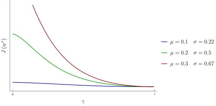
Using the conditions in (5) and (10), we will determine the values of the coefficients $C_{1},C_{2}$ in (9) as well as the optimal values for $\gamma_{1}$ and $\gamma_{2}$. One can check that the (numerical) maxima happen when $\gamma_{1}$ and $\gamma_{2}$ both approach 1 (zero fee). However, the system of equations has no solution as $C_{1}$ and $C_{2}$ are undefined for $\gamma_{1}=\gamma_{2}=1$. Taking the limit as $(\gamma_{1},\gamma_{2})\to(1^{-},1^{-})$, one can show that $J(w,\gamma_{1},\gamma_{2})$ approaches zero, implying that no cost is incurred relative to the optimal strategy.

References

- [1] Adams, H.: Uniswap whitepaper. Tech. rep. (2018)
- [2] Angeris, G., Chitra, T.: Improved price oracles: Constant function market makers. In: Proceedings of the 2nd ACM Conference on Advances in Financial Technologies. p. 80–91. AFT ’20, Association for Computing Machinery, New York, NY, USA (2020). https://doi.org/10.1145/3419614.3423251, https://doi-org.stanford.idm.oclc.org/10.1145/3419614.3423251
- [3] Angeris, G., Evans, A., Chitra, T.: When does the tail wag the dog? Curvature and market making. arXiv preprint arXiv:2012.08040 (2020)
- [4] Angeris, G., Kao, H.T., Chiang, R., Noyes, C., Chitra, T.: An analysis of Uniswap markets. Cryptoeconomic Systems Journal p. to appear (2019)
- [5] Aoyagi, J.: Lazy liquidity in automated market making. Available at SSRN 3674178 (2020)
- [6] Cermak, L.: Uniswap’s monthly trade volume exceeded coinbase’s in september. https://www.theblockcrypto.com/linked/79775/uniswap-coinbase-monthly-volume-september (October 2020)
- [7] Davis, M.H.A., Norman, A.R.: Portfolio selection with transaction costs. Mathematics of Operations Research 15(4), 676–713 (1990), https://EconPapers.repec.org/RePEc:inm:ormoor:v:15:y:1990:i:4:p:676-713
- [8] Dixit, A.: The Art of Smooth Pasting. Fundamentals of pure and applied economics, Harwood Academic Publishers (1993), https://books.google.com/books?id=nmoUDNfYK2sC
- [9] Dixit, A.: A simplified treatment of the theory of optimal regulation of brownian motion. Journal of Economic Dynamics and Control 15(4), 657 – 673 (1991). https://doi.org/https://doi.org/10.1016/0165-1889(91)90037-2, http://www.sciencedirect.com/science/article/pii/0165188991900372
- [10] Dumas, B.: Super contact and related optimality conditions. Journal of Economic Dynamics and Control 15(4), 675–685 (1991), https://EconPapers.repec.org/RePEc:eee:dyncon:v:15:y:1991:i:4:p:675-685
- [11] Dumas, B., Luciano, E.: An exact solution to a dynamic portfolio choice problem under transactions costs. Journal of Finance 46(2), 577–95 (1991), https://EconPapers.repec.org/RePEc:bla:jfinan:v:46:y:1991:i:2:p:577-95
- [12] Dune: Dune analytics decentralized exchange dashboard (2020), available at https://explore.duneanalytics.com/public/dashboards/c87JEtVi2GlyIZHQOR02NsfyJV48eaKEQSiKplJ7
- [13] Evans, A.: Liquidity provider returns in geometric mean markets. arXiv preprint arXiv:2006.08806 (2020)
- [14] Kao, H.T., Chitra, T.: Feedback control as a new primitive for DeFi (2020), https://medium.com/gauntlet-networks/feedback-control-as-a-new-primitive-for-defi-27b493f25b1
- [15] Leland, H.E.: Optimal portfolio management with transactions costs and capital gains taxes. Working Paper RPF-290, IBER, UC Berkeley, Available at SSRN: https://ssrn.com/abstract=206871 (December 1999)
- [16] Martinelli, F., Mushegian, N.: Balancer: A non-custodial portfolio manager, liquidity provider, and price sensor (2019)
- [17] Merton, R.: Lifetime portfolio selection under uncertainty: The continuous-time case. The Review of Economics and Statistics 51(3), 247–57 (1969), https://EconPapers.repec.org/RePEc:tpr:restat:v:51:y:1969:i:3:p:247-57
- [18] Tassy, M., White, D.: Growth rate of a liquidity provider’s wealth in automated market makers. https://math.dartmouth.edu/~mtassy/articles/AMM_returns.pdf (Nov 2020)
Appendix 0.A G3M Arbitrage Results
When the arbitrageur adds reserves of the risky asset, we have the following constant geometric mean formula,
Solving for ,
The aribtrageur’s problem is therefore