MeanShift++: Extremely Fast Mode-Seeking With Applications to Segmentation and Object Tracking

Jennifer Jang
Waymo
jangj@waymo.com Heinrich Jiang
Google Research
heinrichj@google.com

Abstract

MeanShift is a popular mode-seeking clustering algorithm used in a wide range of applications in machine learning. However, it is known to be prohibitively slow, with quadratic runtime per iteration. We propose MeanShift++, an extremely fast mode-seeking algorithm based on MeanShift that uses a grid-based approach to speed up the mean shift step, replacing the computationally expensive neighbors search with a density-weighted mean of adjacent grid cells. In addition, we show that this grid-based technique for density estimation comes with theoretical guarantees. The runtime is linear in the number of points and exponential in dimension, which makes MeanShift++ ideal on low-dimensional applications such as image segmentation and object tracking. We provide extensive experimental analysis showing that MeanShift++ can be more than 10,000x faster than MeanShift with competitive clustering results on benchmark datasets and nearly identical image segmentations as MeanShift. Finally, we show promising results for object tracking.

1 Introduction

MeanShift [20, 22, 31] is a classical mode-seeking clustering algorithm that has a wide range of applications across machine learning and computer vision. Recent applications within computer vision include object tracking [54, 78, 47], unsupervised image segmentation [67, 13, 97], video segmentation [56, 24, 55], image restoration [4, 9], edge-preserving smoothing [55, 8, 12], point clouds [46, 80, 96], and remote sensing [51, 61, 18, 50]. More broadly in machine learning, MeanShift has been used for semi-supervised clustering [2, 73], manifold denoising [86, 82], matrix completion [83, 21], anomaly detection [6, 94, 70], as well as numerous problems in medical imaging [7, 69, 98, 49, 68, 53, 99, 101], wireless sensor networks [95, 100, 89, 64, 85, 62], and robotics [44, 45, 36, 43, 92, 16].

Given a set of examples, MeanShift proceeds in iterations, where in each iteration, each point is moved to the average of the points within a neighborhood ball centered at that point. The radius of the ball is a hyperparameter, often referred to as the bandwidth or window size. All initial examples that converge to the same point are clustered together and the points of convergence are estimates of the modes or local maximas of the probability density function. It has been shown that MeanShift implicitly performs a gradient ascent on the kernel density estimate of the examples [3]. MeanShift thus serves two purposes: mode-seeking and clustering.

MeanShift is often an attractive choice because it is non-parametric: unlike popular objective-based clustering algorithms such as $k$ -means [5, 42] and spectral clustering [52, 79], it does not need to make many assumptions on the data, and the number of clusters is found automatically by the algorithm rather than a hyperparameter that needs to be set. In other words, MeanShift can adapt to general probability distributions. However, one of the main drawbacks of this procedure is its computational complexity: each iteration requires $O(n^{2})$ computations. This is because for each example, calculating the window around the example is linear time in the worst case.

In this paper, we propose MeanShift++, a simple but effective procedure which first partitions the input space into a grid. Then, at each iteration, each point is assigned to its appropriate grid cell. We then approximate any point’s window with the average point in its and its neighboring grid cells. Each iteration in this procedure runs in linear time to the number of data points, with the cost of being exponential to the dimension of the feature space (since the size of the grid is exponential in dimension). Such a trade-off is ideal in settings with a large number of data points but low dimensionality, which is often the case in computer vision applications. With the growing size of modern datasets and increasing resolution of data collected by sensors and cameras, it is becoming ever more urgent to have fast versions of classical techniques.

Our contributions are as follows:

•

We propose MeanShift++, a new mode-seeking procedure based on MeanShift that runs in $O(n\cdot 3^{d})$ per iteration vs $O(n^{2}\cdot d)$ for MeanShift. MeanShift++ has no additional hyperparameters over MeanShift.
•

We show that MeanShift++’s grid-based approximation attains near minimax optimal statistical consistency guarantees at approximating the true density.
•

An extensive empirical analysis shows that MeanShift++ performs at least as well as MeanShift for clustering while being significantly faster.
•

Image segmentation results show that MeanShift++ delivers almost identical segmentations as MeanShift while being as much as 10,000x faster.
•

Image segmentation experiments on the Berkeley Segmentation Dataset Benchmark (BSDS500) found that MeanShift++ performed on par or better than baselines despite being faster than most (and faster than MeanShift by 1,000x).
•

We present a new object tracking algorithm based on MeanShift++ that can adapt to gradual color distributions and scene changes–something most MeanShift-based approaches cannot do due to the computational cost.

2 Related Works

Since MeanShift is a very popular procedure, there have been a number of approaches to speed up the algorithm and other mode-seeking based clustering algorithms in general.

Yang et al. (2003) [91] propose a speedup of MeanShift by using a fast gauss transform to efficiently compute the kernel density estimator, reducing the computational complexity down to linear per iteration; however, they found the fast gauss transform to be impractical for any dimension higher than $3$ . Yang et al. (2005) [90] then applies this technique to a modified similarity function specifically for color histograms and show its effectiveness on frame-tracking in image sequences. Elgamma (2003) [26] also leverage fast gauss transform for color modeling and tracking.

Then there are other computer vision application specific speedup methods for MeanShift. Yin et al. (2011) [93] leverage frame-differences to speed up MeanShift in the specific application of target tracking. Carreira-Perpinan (2006) [13] shows that a spatial discretization strategy can accelerate Gaussian MeanShift image segmentation by one to two orders of magnitude while attaining almost the same segmentation. Carreira-Perpinan [14] also provides similar results for general Gaussian MeanShift; however, in this paper, we show that our method can achieve a far better improvement compared to MeanShift.

Another set of approaches leverage space-partitioning data structures in order to speed up the density estimation calculations. Wang et al. (2007) [81] propose using a dual-tree to obtain a faster approximation of MeanShift with provable accuracy guarantees. Xiao et al. (2010) [88] propose a heuristic to make the computations more efficient by approximating MeanShift using a greatly reduced feature space via applying an adaptive Gaussian KD-Tree.

Freedman et al. (2009) [29] propose speeding up MeanShift by randomly sampling data points when computing the kernel density estimates. This approach only reduces the runtime by small orders and does not address the underlying quadratic runtime issue unless only a small number of samples are used, but this leads to high error in the density estimates. Our method is both linear runtime and utilizes all of the data points to construct an optimal density estimator.

Vedaldi and Soatto (2008) [76] propose a procedure called QuickShift, which is modification of MeanShift in which the trajectories of the points are restricted to the original examples. The same procedure was proposed later by Rodriguez and Laio (2014) [63]. The procedure comes with theoretical guarantees [39], and GPU-based speedups have been proposed for the algorithm [32]. We will show later in the experimental results that QuickShift is indeed much faster than MeanShift, but MeanShift++ is still orders of magnitude faster than QuickShift.

3 Algorithm

We first introduce MeanShift in Algorithm 1 to cluster data points $X_{[n]}:=\{x_{1},..,x_{n}\}$ . The most popular version uses a unit flat kernel (i.e. $K(x):=1[\lVert x\rVert\leq 1]$ [20]), but other kernels can be used as well including the Gaussian kernel [15]. At each iteration, it moves points to its kernel-weighted mean w.r.t. the last iteration’s points until convergence. This computation costs $O(n^{2}\cdot d)$ time per iteration, even if space-partitioning data structures are used to speed up the search to find the $h$ -radius neighborhood in the flat kernel case [88].

Algorithm 1 MeanShift [20, 22, 31]

Inputs: bandwidth

h

, tolerance

\eta

, kernel

K

X_{[n]}

Initialize

y_{0,i}:=x_{i}

for

i\in[n]

t=1

For

i\in[n]

\displaystyle y_{t,i}\leftarrow\frac{\sum_{j\in[n]}K\left(\frac{\lVert y_{t-1,i}-y_{t-1,j}\rVert}{h}\right)y_{t-1,j}}{\sum_{j\in[n]}K\left(\frac{\lVert y_{t-1,i}-y_{t-1,j}\rVert}{h}\right)}.

t\leftarrow t+1

while

\sum_{i=1}^{n}\lVert y_{t,i}-y_{t-1,i}\rVert\geq\eta

return

\{y_{t,1},...,y_{t,n}\}

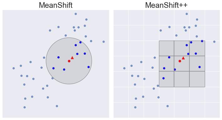
We now introduce MeanShift++ (Algorithm 2). In each iteration, it first performs a preprocessing step of parititioning the input data points into appropriate grid cells, which are hypercubes of side length $h$ . A graphical comparison with MeanShift is shown in Figure 1. In practice, we keep two hash tables $\mathcal{C}$ (to store the count in each cell) and $\mathcal{S}$ (to store the sum in each cell). $\mathcal{C}$ and $\mathcal{S}$ are defined as initially empty mappings from lattice points in $D$ -dimension (corresponding to grid cells) to non-negative integers and $\mathbb{R}^{D}$ respectively. We show how they are updated via a single pass through the dataset.

To compute which grid cell an example belongs to, we first divide each entry by $h$ and then take the element-wise floor function, which gives a $d$ -dimensional integer vector index of the grids. Then, we can simply use the preprocessed information in the point’s grid cell and neighboring grid cells to compute the shifted point. As a result, each point is moved to the average of all the points within its cell and neighboring cells. This grid-based approach is a much faster approximation of the density at low dimensions. The runtime of MeanShift++ grows linearly with $n$ , while MeanShift is quadratic (Figure 2).

Algorithm 2 MeanShift++

Inputs: bandwidth

h

, tolerance

\eta

X_{[n]}

Initialize

y_{0,i}:=x_{i}

for

i\in[n]

t=1

Initialize empty hash tables

\mathcal{C}:\mathcal{Z}^{d}\rightarrow\mathcal{Z}_{\geq 0}

(stores cell count),

\mathcal{S}:\mathcal{Z}^{d}\rightarrow\mathbb{R}^{d}

(stores cell sum).

\mathcal{C}(\lfloor y_{t-1,i}/h\rfloor)\leftarrow\mathcal{C}(\lfloor y_{t-1,i}/h\rfloor)+1

for

i\in[n]

\mathcal{S}(\lfloor y_{t-1,i}/h\rfloor)\leftarrow\mathcal{S}(\lfloor y_{t-1,i}/h\rfloor)+y_{t-1,i}

for

i\in[n]

Next, for all

i\in[n]

\displaystyle y_{t,i}\leftarrow\frac{\sum_{v\in\{-1,0,1\}^{d}}\mathcal{S}(\lfloor y_{t-1,i}/h\rfloor+v)}{\sum_{v\in\{-1,0,1\}^{d}}\mathcal{C}(\lfloor y_{t-1,i}/h\rfloor+v)}.

t\leftarrow t+1

while

\sum_{i=1}^{n}\lVert y_{t,i}-y_{t-1,i}\rVert\geq\eta

return

\{y_{t,1},...,y_{t,n}\}

Refer to caption — Figure 1: 2D example illustrating the difference between MeanShift and MeanShift++. The red circle is the point we want to shift to the mean of its neighbors. It takes $O(n)$ for MeanShift to find the neighbors of a single point versus $O(3^{d})$ for MeanShift++ using grid cells. The location of the new point is indicated by the red triangle.

4 Theory

In this section, we give guarantees on our grid-based approach. Suppose there is some underlying distribution $\mathcal{P}$ with corresponding density function $p:\mathbb{R}^{d}\rightarrow\mathbb{R}_{\geq 0}$ from which our data points $X_{[n]}=\{x_{1},...,x_{n}\}$ are drawn i.i.d. We show guarantees on the density estimator based on the grid cell counts.

We need the following regularity assumptions on the density function. The first ensures that the density function has compact support with smooth boundaries and is lower bounded by some positive quantity, and the other ensures that the density function has smoothness. These are standard assumptions in analyses on density estimation e.g. [35, 40, 19, 65].

Assumption 1.

$p$ has compact support $\mathcal{X}\in\mathbb{R}^{d}$ and there exists $\lambda_{0},r_{0},C_{0}>0$ such that $p(x)\geq\lambda_{0}$ for all $x\in\mathcal{X}$ and $\text{Vol}(B(x,r)\cap\mathcal{X})\geq C_{0}\cdot\text{Vol}(B(x,r))$ for all $x\in\mathcal{X}$ and $0<r\leq r_{0}$ , where $B(x,r):=\{x^{\prime}\in\mathbb{R}^{d}:|x-x^{\prime}|\leq r\}$ .

Assumption 2.

$p$ is $\alpha$ -Hölder continuous for some $0<\alpha\leq 1$ : i.e. there exists $C_{\alpha}>0$ such that $|p(x)-p(x^{\prime})|\leq C_{\alpha}\cdot|x-x^{\prime}|^{\alpha}$ for all $x,x^{\prime}\in\mathbb{R}^{d}$ .

We now give the result, which says that for $h$ sufficiently small depending on $p$ (if $h$ is too large, then the grid is too coarse to learn a statistically consistent density estimator), and $n$ sufficiently large, there will be a high probability finite-sample uniform bound on the difference between the density estimator and the true density. The proof can be found in the Appendix.

Theorem 1.

Suppose Assumption 1 and 2 hold. Then there exists constants $C,C_{1}>0$ depending on $p$ such that the following holds. Let $0<\delta<1$ , $0<h<\text{min}\{\left(\frac{\lambda_{0}}{2\cdot C_{\alpha}}\right)^{1/\alpha},r_{0}\}$ , $nh^{d}\geq C_{1}$ . Let $\mathcal{G}_{h}$ be a partitioning of $\mathbb{R}^{d}$ into grid cells of edge-length $h$ and for $x\in\mathbb{R}^{d}$ . Let $G(x)$ denote the cell in $\mathcal{G}_{h}$ that $x$ belongs to. Then, define the corresponding density estimator $\widehat{p}_{h}$ as:

\displaystyle\widehat{p}_{h}(x):=\frac{|X_{[n]}\cap G(x)|}{n\cdot h^{d}}.

Then, with probability at least $1-\delta$ :

\displaystyle\sup_{x\in\mathbb{R}^{d}}|\widehat{p}_{h}(x)-p(x)|\leq C\cdot\left(h^{\alpha}+\frac{\sqrt{\log(1/(h\delta)}}{\sqrt{n\cdot h^{d}}}\right).

Remark 1.

In the above result, choosing $h\approx n^{-1/(2\alpha+d)}$ optimizes the convergence rate to $\tilde{O}(n^{-\alpha/(2\alpha+d)})$ , which is the minimax optimal convergence up to logarithmic factors for the density estimation problem as established by Tsybakov [72, 71].

In other words, the grid-based approach statistically performs at least as well as any estimator of the density function, including the density estimator used by MeanShift. It is worth noting that while our results only provide results for the density estimation portion of MeanShift++ (i.e. the grid-cell binning technique), we prove the near-minimax optimality of this estimation. This implies that the information contained in the density estimation portion serves as an approximately sufficient statistic for the rest of the procedure, which behaves similarly to MeanShift, which operates on another, also nearly-optimal density estimator. Thus, existing analyses of MeanShift e.g. [3, 17, 87, 48, 34, 33, 66] can be adapted here; however, it is known that MeanShift is very difficult to analyze [23] and a complete analysis is beyond the scope of this paper.

	Dataset	$n$	$d$	$c$
a	Phone Accelerometer	13,062,475	3	7
b	Phone Gyroscope	13,932,632	3	7
c	Watch Accelerometer	3,540,962	3	7
d	Watch Gyroscope	3,205,431	3	7
e	Still	949,983	3	6
f	Skin	245,057	3	2
g	Iris	150	4	3
h	Lupus	87	3	2
i	Confidence	72	3	2
j	Geyser	22	2	2
k	Balance Scale	625	4	3
l	Vinnie	380	2	2
m	Sleep Data	1,024	2	2
n	Transplant	131	3	2
o	Slope	44	3	2
p	PRNN	250	2	2
q	Wall Robot	5,456	4	4
r	User Knowledge	403	5	5

Table 1: Summary of datasets used. Includes dataset size (

n

), number of features (

d

), and number of clusters (

c

	ARI		AMI
	MS++	MS	MS++	MS
a) Phone	0.0897	DNF	0.1959	DNF
Accelerometer	29m 59s	$>$ 24h	49m 19s	$>$ 24h
b) Phone	0.2354	DNF	0.1835	DNF
Gyroscope	1h 35m	$>$ 24h	32m 32s	$>$ 24h
c) Watch	0.0913	DNF	0.2309	DNF
Accelerometer	17m 52s	$>$ 24h	43m 32s	$>$ 24h
d) Watch	0.1595	DNF	0.1336	DNF
Gyroscope	24m 45s	$>$ 24h	9m 3s	$>$ 24h
e) Still	0.7900	DNF	0.8551	DNF
	13.12s	$>$ 24h	8.58s	$>$ 24h
f) Skin	0.3270	0.3255	0.4240	0.3975
	16.44s	3h 41m	13.07s	3h 41m
g) Iris	0.5681	0.6832	0.7316	0.6970
	$<$ 0.01s	6.35s	$<$ 0.01s	2.36s
h) Lupus	0.1827	0.1399	0.2134	0.2042
	$<$ 0.01s	3.82s	$<$ 0.01s	3.82s
i) Confidence	0.2080	0.2059	0.2455	0.2215
	0.02s	0.70s	$<$ 0.01s	0.98s
j) Geyser	0.1229	0.0886	0.2409	0.2198
	$<$ 0.01s	2.88s	$<$ 0.01s	2.88s
k) Balance Scale	0.0883	0.0836	0.2268	0.2166
	0.09s	16.02s	0.09s	16.02s
l) Vinnie	0.4594	0.4383	0.3666	0.3671
	0.01s	16.85s	0.01s	16.85s
m) Sleep Data	0.1181	0.1242	0.1028	0.0998
	0.02s	45.25s	0.02s	45.25s
n) Transplant	0.7687	0.6328	0.7175	0.7018
	$<$ 0.01s	4.22s	$<$ 0.01s	4.22s
o) Slope	0.2777	0.2715	0.3877	0.3630
	$<$ 0.01s	0.43s	$<$ 0.01s	0.43s
p) PRNN	0.2093	0.1872	0.2912	0.2590
	0.02s	10.72s	$<$ 0.01s	10.72s
q) Wall Robot	0.1788	0.1706	0.3239	0.3246
	0.69s	4m37s	0.88s	2m30s
r) User Knowledge	0.3398	0.2140	0.4086	0.3278
	0.06s	7.62s	0.06s	7.62s

Table 2: Summary of clustering performances. MeanShift++’s and MeanShift’s best results for 19 real-world datasets after tuning bandwidth. Datasets from the UCI Machine Learning Repository [25] and OpenML [75]. In cases where the original target variable is continuous, binarized versions of the datasets were used. These experiments were run on a local machine with a 1.2 GHz Intel Core M processor and 8 GB memory. MeanShift did not finish (DNF) within 24 hours for the top five largest datasets. ARI, AMI, and runtime are reported for each run, and the highest score obtained for that metric and dataset is bolded.

	Average Runtime ( $\mu s$ )
MeanShift++	2,675,100
MeanShift	1,765,462,893
SLIC	56,266
Quickshift	31,717,386

5 Experiments

We compare Meanshift++ against MeanShift on various clustering tasks in Table 1. These comparisons are made using the Scikit-Learn [57] implementation of MeanShift and our own implementation of MeanShift++ in Cython.

To measure the quality of a clustering result, we use the Adjusted Rand Index (ARI) [37] and the Adjusted Mutual Information (AMI) [77] scores, which compare the clustering with the partitioning induced by the labels of the data points, a popular way of comparing clustering performance [38]. The benchmark datasets we use are labeled datasets, and we only cluster the features.

As stated earlier, MeanShift++ is linear with respect to the number of data points and exponential in dimension. We thus show results on low-dimensional datasets. In Figure 3, we ran both algorithms on 19 benchmark datasets with $5$ or fewer dimensions, ranging from less than $100$ data points to millions of data points.

For the top five largest datasets, MeanShift failed to return a result for any setting of bandwidth despite running for more than 24 hours. MeanShift++ consistently outperformed MeanShift in both clustering quality and runtime for the rest of the datasets, as shown in Table 2. We saw a significant speed reduction of over 100x on both small and large datasets, showing that MeanShift++ does not have significantly more overhead costs than MeanShift either.

We also show in Figure 3 the effect the bandwidth setting has on clustering performance and runtime for a few of the datasets to provide further insight into the stability of the procedures under the bandwidth hyperparameter.

We note that MeanShift++ outperforms MeanShift on many datasets, possibly due to a regularizing effect: by partitioning the space into grids and assigning every point in the same cell the same value instead of a unique value for each point, the gradient-ascent shifting step is more stable than in MeanShift. This regularization effect, combined with the option to tune the cell-length which essentially controls the amount of regularization, allows MeanShift++ to outperform Meanshift in some cases.

However, these results are unlikely to generalize to higher dimensions. It is known that density-based procedures perform poorly in high dimensions due to the curse of dimensionality. Our theoretical results also show that rates become exponentially worse in higher dimension.

6 Image Segmentation

We compare MeanShift++ to a number of baselines for unsupervised image segmentation in Figure 4. We include Felzenszwalb [27], QuickShift [76], and $k$ -means, three popular image segmentation procedures from the Python Scikit-Image library [74], as well as Quickshift++ [41], a recent algorithm shown to be an improvement over Quickshift on image segmentation. We also include MeanShift, which often produces qualitatively better clusters than the other baselines, but runs for so much longer that it is impractical for high-resolution image segmentation.

For image segmentation, we run each algorithm on a preprocessed image with each pixel represented in a 3D RGB color channel space, with the exception of Quickshift++, which takes $(r,g,b,x,y)$ color and spatial coordinates. MeanShift was run with both $(r,g,b)$ (shown in Figure 4) and $(r,g,b,x,y)$ inputs, but we did not see a difference in segmentation quality or runtime. For each algorithm, the returned clusters are taken as the segments.

Our image segmentation experiments in Figure 4 show that MeanShift++ is able to produce segmentations that are nearly identical to that of MeanShift with an up to 10,000x speedup. We capped the sizes of our images at 187,500 pixels to allow MeanShift to finish running, so this speedup would surely be greater on even higher resolution images.

Multiple attempts have been made to speed up MeanShift for image segmentation at the cost of quality, but MeanShift++ does not seem to trade off segmentation quality despite running in a sub-fraction of the time.

For a more quantitative comparison, we ran experiments using the Berkeley Segmentation Dataset Benchmark (BSDS500) of $500$ images with $6$ human-labeled segmentations each. We ran MeanShift++, MeanShift, SLIC, and QuickShift on each image and used the adjusted RAND index [37] (ARI) and Fowlkes-Mallows [28] (FM) scores to compare the clusters. Scores were averaged over the $6$ ground truth segmentations. We found that MeanShift++ performed on par or better than baselines despite being faster than MeanShift by 1,000x on average (Figure 6).

7 Object Tracking

The mode-seeking behavior of MeanShift makes it a good candidate for visual tracking. A basic implementation would take in a mask and/or search window of an object and build a histogram of the colors found in that object in RGB or HSV space. Afterwards, the histogram is normalized by the colors found in surrounding, non-target points into a probability distribution. At each step, the tracking algorithm would backproject each point in the window into a probability that it is part of the original object. The center of the window moves in $(x,y)$ space to the mode of the distribution within the window until convergence in the same way that MeanShift iteratively moves each point to the mean of its neighbors. Every frame thereafter would be initialized with the final window of the previous frame.

Algorithm 3 MeanShift++ for Tracking

Inputs: bandwidth

h

, tolerance

\eta

, initial window

W_{0}

, sequence of frames

X_{0},X_{1},...,X_{T}

Define:

W\cap X

as pixels in window

W

for frame

X

Run MeanShift++ on the pixels (in color space) in

W_{0}\cap X_{0}

and manually select the cluster(s) desired to track. Let the union of selected cluster(s) be

C

B\leftarrow\{\lfloor c/h\rfloor:c\in C\}

for

i=1,2,...,T

Initialize

W_{i}\leftarrow W_{i-1}

R_{i}:=\{x\in W_{i}\cap X_{i}:\lfloor x/h\rfloor\in B\}

Move

W_{i}

so that it’s centered at the average

(x,y)

-position of points in

R_{i}

while

W_{i}

’s center converges with tolerance

\eta

Optionally update

B\leftarrow\{\lfloor x/h\rfloor:x\in W_{i}\cap X_{i}\}\cap N(B)

, where

N(B)

are all cells that are in

B

or adjacent to one in

B

emit

W_{i}

for frame

X_{i}

MeanShift++ can be used for object tracking in a similar, albeit more principled way (Algorithm 3). Instead of color histograms, which need to be computed and require extra hyperparameters to determine the size of bins, the grid cells generated by MeanShift++ during clustering are already precomputed and suitable for tracking: we can quickly compute which points fall into any bin belonging to the target cluster(s).

MeanShift is also too slow to generate masks needed for real-time tracking. It often requires the user to provide a precomputed mask or color range. Relying on user input is imperfect and subject to biases. MeanShift++ is fast enough to generate masks through real-time clustering.

Off-the-shelf versions of MeanShift tracking rely on a histogram calculated from the original frame throughout the whole scene. This does not work well if the illumination in the scene changes, since the algorithm cannot make fast updates to the histogram [30, 84, 58, 59]. MeanShift++ can adapt to changing color distributions by finding and adding neighboring grids of points to the histogram in linear time, making it more robust to gradual changes in lighting, color, and other artifacts of the data.

CamShift [11, 1] improves MeanShift tracking by adjusting window sizes as objects move closer or farther away and updating color histograms based on lighting changes, among other things. Future work may involve adapting these ideas to a MeanShift++-based tracking algorithm.

In Figure 5, we show the performance of MeanShift++ and MeanShift (from the Python OpenCV library [10]) on object tracking in various scenes. In practice, we found that MeanShift tends to be easily misled by the surroundings, particularly when there are areas of similar color. Finally, MeanShift++ usually finds better windows than MeanShift.

8 Conclusion

We provided MeanShift++, a simple and principled approach to speed up the MeanShift algorithm in low-dimensional settings. We applied it to clustering, image segmentation, and object tracking, and show that MeanShift++ is competitive with MeanShift in low dimensions while being as much as 10,000x faster. This dramatic speedup makes MeanShift++ practical for modern computer vision applications.

References

[1] John G Allen, Richard YD Xu, Jesse S Jin, et al. Object tracking using camshift algorithm and multiple quantized feature spaces. In ACM International Conference Proceeding Series, volume 100, pages 3–7. Citeseer, 2004.
[2] Saket Anand, Sushil Mittal, Oncel Tuzel, and Peter Meer. Semi-supervised kernel mean shift clustering. IEEE transactions on pattern analysis and machine intelligence, 36(6):1201–1215, 2013.
[3] Ery Arias-Castro, David Mason, and Bruno Pelletier. On the estimation of the gradient lines of a density and the consistency of the mean-shift algorithm. The Journal of Machine Learning Research, 17(1):1487–1514, 2016.
[4] Siavash Arjomand Bigdeli, Matthias Zwicker, Paolo Favaro, and Meiguang Jin. Deep mean-shift priors for image restoration. Advances in Neural Information Processing Systems, 30:763–772, 2017.
[5] David Arthur and Sergei Vassilvitskii. k-means++: The advantages of careful seeding. Technical report, Stanford, 2006.
[6] Ilhan Aydin, Mehmet Karaköse, and Erhan Akin. A robust anomaly detection in pantograph-catenary system based on mean-shift tracking and foreground detection. In 2013 IEEE international conference on systems, man, and cybernetics, pages 4444–4449. IEEE, 2013.
[7] Pei Rui Bai, Qing Yi Liu, Lei Li, Sheng Hua Teng, Jing Li, and Mao Yong Cao. A novel region-based level set method initialized with mean shift clustering for automated medical image segmentation. Computers in biology and medicine, 43(11):1827–1832, 2013.
[8] Danny Barash and Dorin Comaniciu. A common framework for nonlinear diffusion, adaptive smoothing, bilateral filtering and mean shift. Image and Vision Computing, 22(1):73–81, 2004.
[9] Siavash Arjomand Bigdeli and Matthias Zwicker. Image restoration using autoencoding priors. arXiv preprint arXiv:1703.09964, 2017.
[10] Gary Bradski and Adrian Kaehler. Learning OpenCV: Computer vision with the OpenCV library. ” O’Reilly Media, Inc.”, 2008.
[11] Gary R Bradski. Computer vision face tracking for use in a perceptual user interface. 1998.
[12] Torsten Büschenfeld and Jörn Ostermann. Edge preserving land cover classification refinement using mean shift segmentation. Proceedings Of The 4th GEOBIA, 2012.
[13] Miguel A Carreira-Perpinan. Acceleration strategies for gaussian mean-shift image segmentation. In 2006 IEEE Computer Society Conference on Computer Vision and Pattern Recognition (CVPR’06), volume 1, pages 1160–1167. IEEE, 2006.
[14] Miguel Á Carreira-Perpiñán. Fast nonparametric clustering with gaussian blurring mean-shift. In Proceedings of the 23rd international conference on Machine learning, pages 153–160, 2006.
[15] Miguel A Carreira-Perpinan. Gaussian mean-shift is an em algorithm. IEEE Transactions on Pattern Analysis and Machine Intelligence, 29(5):767–776, 2007.
[16] Young-Su Cha, KangGeon Kim, Ji-Yong Lee, Joongjae Lee, Minjun Choi, Mun-Ho Jeong, ChangHwan Kim, Bum-Jae You, and Sang-Rok Oh. Mahru-m: A mobile humanoid robot platform based on a dual-network control system and coordinated task execution. Robotics and Autonomous Systems, 59(6):354–366, 2011.
[17] Ting-Li Chen. On the convergence and consistency of the blurring mean-shift process. Annals of the Institute of Statistical Mathematics, 67(1):157–176, 2015.
[18] Wei Chen, Xingbo Hu, Wen Chen, Yifeng Hong, and Minhua Yang. Airborne lidar remote sensing for individual tree forest inventory using trunk detection-aided mean shift clustering techniques. Remote Sensing, 10(7):1078, 2018.
[19] Yen-Chi Chen. A tutorial on kernel density estimation and recent advances. Biostatistics & Epidemiology, 1(1):161–187, 2017.
[20] Yizong Cheng. Mean shift, mode seeking, and clustering. IEEE transactions on pattern analysis and machine intelligence, 17(8):790–799, 1995.
[21] Sunav Choudhary, Naveen Kumar, Srikanth Narayanan, and Urbashi Mitra. Active target localization using low-rank matrix completion and unimodal regression. arXiv preprint arXiv:1601.07254, 2016.
[22] Dorin Comaniciu and Peter Meer. Mean shift analysis and applications. In Proceedings of the Seventh IEEE International Conference on Computer Vision, volume 2, pages 1197–1203. IEEE, 1999.
[23] Sanjoy Dasgupta and Samory Kpotufe. Optimal rates for k-nn density and mode estimation. In Advances in Neural Information Processing Systems, pages 2555–2563, 2014.
[24] Daniel DeMenthon and Remi Megret. Spatio-temporal segmentation of video by hierarchical mean shift analysis. Citeseer, 2002.
[25] Dheeru Dua and Casey Graff. UCI machine learning repository, 2017.
[26] Ahmed Elgammal, Ramani Duraiswami, and Larry S Davis. Efficient kernel density estimation using the fast gauss transform with applications to color modeling and tracking. IEEE transactions on pattern analysis and machine intelligence, 25(11):1499–1504, 2003.
[27] Pedro F Felzenszwalb and Daniel P Huttenlocher. Efficient graph-based image segmentation. International journal of computer vision, 59(2):167–181, 2004.
[28] Edward B Fowlkes and Colin L Mallows. A method for comparing two hierarchical clusterings. Journal of the American statistical association, 78(383):553–569, 1983.
[29] Daniel Freedman and Pavel Kisilev. Fast mean shift by compact density representation. In 2009 IEEE Conference on Computer Vision and Pattern Recognition, pages 1818–1825. IEEE, 2009.
[30] Daniel Freedman and Matthew W Turek. Illumination-invariant tracking via graph cuts. In 2005 IEEE Computer Society Conference on Computer Vision and Pattern Recognition (CVPR’05), volume 2, pages 10–17. IEEE, 2005.
[31] Keinosuke Fukunaga and Larry Hostetler. The estimation of the gradient of a density function, with applications in pattern recognition. IEEE Transactions on information theory, 21(1):32–40, 1975.
[32] Brian Fulkerson and Stefano Soatto. Really quick shift: Image segmentation on a gpu. In European Conference on Computer Vision, pages 350–358. Springer, 2010.
[33] Youness Aliyari Ghassabeh. On the convergence of the mean shift algorithm in the one-dimensional space. Pattern Recognition Letters, 34(12):1423–1427, 2013.
[34] Youness Aliyari Ghassabeh. A sufficient condition for the convergence of the mean shift algorithm with gaussian kernel. Journal of Multivariate Analysis, 135:1–10, 2015.
[35] Evarist Giné and Armelle Guillou. Rates of strong uniform consistency for multivariate kernel density estimators. In Annales de l’Institut Henri Poincare (B) Probability and Statistics, volume 38, pages 907–921. Elsevier, 2002.
[36] Jwu-Sheng Hu, Jyun-Ji Wang, and Daniel Minare Ho. Design of sensing system and anticipative behavior for human following of mobile robots. IEEE Transactions on Industrial Electronics, 61(4):1916–1927, 2013.
[37] Lawrence Hubert and Phipps Arabie. Comparing partitions. Journal of classification, 2(1):193–218, 1985.
[38] Jennifer Jang and Heinrich Jiang. Dbscan++: Towards fast and scalable density clustering. In International Conference on Machine Learning, pages 3019–3029. PMLR, 2019.
[39] Heinrich Jiang. On the consistency of quick shift. In Advances in Neural Information Processing Systems, pages 46–55, 2017.
[40] Heinrich Jiang. Uniform convergence rates for kernel density estimation. In International Conference on Machine Learning, pages 1694–1703, 2017.
[41] Heinrich Jiang, Jennifer Jang, and Samory Kpotufe. Quickshift++: Provably good initializations for sample-based mean shift. arXiv preprint arXiv:1805.07909, 2018.
[42] Tapas Kanungo, David M Mount, Nathan S Netanyahu, Christine D Piatko, Ruth Silverman, and Angela Y Wu. An efficient k-means clustering algorithm: Analysis and implementation. IEEE transactions on pattern analysis and machine intelligence, 24(7):881–892, 2002.
[43] Masato Kato, Yuichi Kobayashi, and Shigeyuki Hosoe. Optimizing resolution for feature extraction in robotic motion learning. In 2005 IEEE International Conference on Systems, Man and Cybernetics, volume 2, pages 1086–1091. IEEE, 2005.
[44] Oliver Kroemer, Renaud Detry, Justus Piater, and Jan Peters. Active learning using mean shift optimization for robot grasping. In 2009 IEEE/RSJ International Conference on Intelligent Robots and Systems, pages 2610–2615. IEEE, 2009.
[45] Rolf Lakaemper. Simultaneous multi-line-segment merging for robot mapping using mean shift clustering. In 2009 IEEE/RSJ International Conference on Intelligent Robots and Systems, pages 1654–1660. IEEE, 2009.
[46] I-Chieh Lee, Bo Wu, and Ron Li. Shoreline extraction from the integration of lidar point cloud data and aerial orthophotos using mean-shift segmentation. In Proc. ASPRS Annual Conf, volume 2, pages 3033–3040, 2009.
[47] Ido Leichter, Michael Lindenbaum, and Ehud Rivlin. Mean shift tracking with multiple reference color histograms. Computer Vision and Image Understanding, 114(3):400–408, 2010.
[48] Xiangru Li, Zhanyi Hu, and Fuchao Wu. A note on the convergence of the mean shift. Pattern recognition, 40(6):1756–1762, 2007.
[49] Arnaldo Mayer and Hayit Greenspan. An adaptive mean-shift framework for mri brain segmentation. IEEE transactions on medical imaging, 28(8):1238–1250, 2009.
[50] Julien Michel, David Youssefi, and Manuel Grizonnet. Stable mean-shift algorithm and its application to the segmentation of arbitrarily large remote sensing images. IEEE Transactions on Geoscience and Remote Sensing, 53(2):952–964, 2014.
[51] Dongping Ming, Tianyu Ci, Hongyue Cai, Longxiang Li, Cheng Qiao, and Jinyang Du. Semivariogram-based spatial bandwidth selection for remote sensing image segmentation with mean-shift algorithm. IEEE Geoscience and Remote Sensing Letters, 9(5):813–817, 2012.
[52] Andrew Y Ng, Michael I Jordan, and Yair Weiss. On spectral clustering: Analysis and an algorithm. In Advances in neural information processing systems, pages 849–856, 2002.
[53] Binh P Nguyen, Wei-Liang Tay, Chee-Kong Chui, and Sim-Heng Ong. A clustering-based system to automate transfer function design for medical image visualization. The Visual Computer, 28(2):181–191, 2012.
[54] Jifeng Ning, Lei Zhang, David Zhang, and Chengke Wu. Robust mean-shift tracking with corrected background-weighted histogram. IET computer vision, 6(1):62–69, 2012.
[55] Sylvain Paris. Edge-preserving smoothing and mean-shift segmentation of video streams. In European Conference on Computer Vision, pages 460–473. Springer, 2008.
[56] Sylvain Paris and Frédo Durand. A topological approach to hierarchical segmentation using mean shift. In 2007 IEEE Conference on Computer Vision and Pattern Recognition, pages 1–8. IEEE, 2007.
[57] Fabian Pedregosa, Gaël Varoquaux, Alexandre Gramfort, Vincent Michel, Bertrand Thirion, Olivier Grisel, Mathieu Blondel, Peter Prettenhofer, Ron Weiss, Vincent Dubourg, et al. Scikit-learn: Machine learning in python. the Journal of machine Learning research, 12:2825–2830, 2011.
[58] Gargi Phadke and Rajbabu Velmurgan. Illumination invariant mean-shift tracking. In 2013 IEEE Workshop on Applications of Computer Vision (WACV), pages 407–412. IEEE, 2013.
[59] Gargi Phadke and Rajbabu Velmurugan. Mean lbp and modified fuzzy c-means weighted hybrid feature for illumination invariant mean-shift tracking. Signal, Image and Video Processing, 11(4):665–672, 2017.
[60] Jeff M Phillips. Chernoff-hoeffding inequality and applications. arXiv preprint arXiv:1209.6396, 2012.
[61] Moacir P Ponti. Segmentation of low-cost remote sensing images combining vegetation indices and mean shift. IEEE Geoscience and Remote Sensing Letters, 10(1):67–70, 2012.
[62] Hongchun Qu, Zeliang Qiu, Xiaoming Tang, Min Xiang, and Ping Wang. Incorporating unsupervised learning into intrusion detection for wireless sensor networks with structural co-evolvability. Applied Soft Computing, 71:939–951, 2018.
[63] Alex Rodriguez and Alessandro Laio. Clustering by fast search and find of density peaks. Science, 344(6191):1492–1496, 2014.
[64] Saunhita Sapre and S Mini. Moth flame based optimized placement of relay nodes for fault tolerant wireless sensor networks. In 2018 9th International Conference on Computing, Communication and Networking Technologies (ICCCNT), pages 1–6. IEEE, 2018.
[65] Aarti Singh, Clayton Scott, Robert Nowak, et al. Adaptive hausdorff estimation of density level sets. The Annals of Statistics, 37(5B):2760–2782, 2009.
[66] Raghav Subbarao and Peter Meer. Nonlinear mean shift over riemannian manifolds. International journal of computer vision, 84(1):1, 2009.
[67] Wenbing Tao, Hai Jin, and Yimin Zhang. Color image segmentation based on mean shift and normalized cuts. IEEE Transactions on Systems, Man, and Cybernetics, Part B (Cybernetics), 37(5):1382–1389, 2007.
[68] Huseyin Tek, Alper Ayvaci, and Dorin Comaniciu. Method and apparatus for detecting blood vessel boundaries using multi-scale mean-shift ray propagation, Aug. 10 2010. US Patent 7,773,787.
[69] Huseyin Tek, Dorin Comaniciu, and James P Williams. Vessel detection by mean shift based ray propagation. In Proceedings IEEE Workshop on Mathematical Methods in Biomedical Image Analysis (MMBIA 2001), pages 228–235. IEEE, 2001.
[70] Du-Ming Tsai and Jie-Yu Luo. Mean shift-based defect detection in multicrystalline solar wafer surfaces. IEEE Transactions on Industrial Informatics, 7(1):125–135, 2010.
[71] Alexandre B Tsybakov. Introduction to nonparametric estimation. Springer Science & Business Media, 2008.
[72] Alexandre B Tsybakov et al. On nonparametric estimation of density level sets. The Annals of Statistics, 25(3):948–969, 1997.
[73] Oncel Tuzel, Fatih Porikli, and Peter Meer. Kernel methods for weakly supervised mean shift clustering. In 2009 IEEE 12th International Conference on Computer Vision, pages 48–55. IEEE, 2009.
[74] Stefan Van der Walt, Johannes L Schönberger, Juan Nunez-Iglesias, François Boulogne, Joshua D Warner, Neil Yager, Emmanuelle Gouillart, and Tony Yu. scikit-image: image processing in python. PeerJ, 2:e453, 2014.
[75] Joaquin Vanschoren, Jan N. van Rijn, Bernd Bischl, and Luis Torgo. Openml: Networked science in machine learning. SIGKDD Explorations, 15(2):49–60, 2013.
[76] Andrea Vedaldi and Stefano Soatto. Quick shift and kernel methods for mode seeking. In European conference on computer vision, pages 705–718. Springer, 2008.
[77] Nguyen Xuan Vinh, Julien Epps, and James Bailey. Information theoretic measures for clusterings comparison: Variants, properties, normalization and correction for chance. The Journal of Machine Learning Research, 11:2837–2854, 2010.
[78] Tomas Vojir, Jana Noskova, and Jiri Matas. Robust scale-adaptive mean-shift for tracking. Pattern Recognition Letters, 49:250–258, 2014.
[79] Ulrike Von Luxburg. A tutorial on spectral clustering. Statistics and computing, 17(4):395–416, 2007.
[80] George Vosselman. Point cloud segmentation for urban scene classification. Int. Arch. Photogramm. Remote Sens. Spat. Inf. Sci, 1:257–262, 2013.
[81] Ping Wang, Dongryeol Lee, Alexander Gray, and James M Rehg. Fast mean shift with accurate and stable convergence. In Artificial Intelligence and Statistics, pages 604–611, 2007.
[82] Weiran Wang and Miguel A Carreira-Perpinán. Manifold blurring mean shift algorithms for manifold denoising. In 2010 IEEE Computer Society Conference on Computer Vision and Pattern Recognition, pages 1759–1766. IEEE, 2010.
[83] Weiran Wang, Miguel A Carreira-Perpinán, and Zhengdong Lu. A denoising view of matrix completion. In Advances in Neural Information Processing Systems, pages 334–342, 2011.
[84] Inteck Whoang, Jeong Heon Kim, and Kwang Nam Choi. Object tracking using maximum colour distance under illumination change. International Journal of Advanced Robotic Systems, 9(5):212, 2012.
[85] Dalei Wu, Song Ci, Haiyan Luo, Yun Ye, and Haohong Wang. Video surveillance over wireless sensor and actuator networks using active cameras. IEEE Transactions on Automatic Control, 56(10):2467–2472, 2011.
[86] Yunhua Xiang and Yen-Chi Chen. Statistical inference using mean shift denoising. arXiv preprint arXiv:1610.03927, 2016.
[87] LI Xiang-Ru, WU Fu-Chao, and HU Zhan-Yi. Convergence of a mean shift algorithm. 2005.
[88] Chunxia Xiao and Meng Liu. Efficient mean-shift clustering using gaussian kd-tree. In Computer Graphics Forum, volume 29, pages 2065–2073. Wiley Online Library, 2010.
[89] Qing Yan Xie and Yizong Cheng. K-centers mean-shift reverse mean-shift clustering algorithm over heterogeneous wireless sensor networks. In 2014 Wireless Telecommunications Symposium, pages 1–6. IEEE, 2014.
[90] Changjiang Yang, Ramani Duraiswami, and Larry Davis. Efficient mean-shift tracking via a new similarity measure. In 2005 IEEE Computer Society Conference on Computer Vision and Pattern Recognition (CVPR’05), volume 1, pages 176–183. IEEE, 2005.
[91] Changjiang Yang, Ramani Duraiswami, Nail A Gumerov, and Larry Davis. Improved fast gauss transform and efficient kernel density estimation. IEEE, 2003.
[92] Tao Yang, Chee Kong Chui, Jiang Liu, Weimin Huang, Yi Su, and Stephen KY Chang. Robotic learning of motion using demonstrations and statistical models for surgical simulation. International journal of computer assisted radiology and surgery, 9(5):813–823, 2014.
[93] Hongpeng Yin, Yi Chai, Simon X Yang, and Xiaoyan Yang. Fast-moving target tracking based on mean shift and frame-difference methods. Journal of Systems Engineering and Electronics, 22(4):587–592, 2011.
[94] Li Yu and Zhiling Lan. A scalable, non-parametric anomaly detection framework for hadoop. In Proceedings of the 2013 ACM Cloud and Autonomic Computing Conference, pages 1–2, 2013.
[95] Xiaosheng Yu, Jianning Chi, Ying Wang, and Hao Chu. Mean shift-based multisource localization method in wireless binary sensor network. Journal of Sensors, 2020, 2020.
[96] Wenlong Yue, Junguo Lu, Weihang Zhou, and Yubin Miao. A new plane segmentation method of point cloud based on mean shift and ransac. In 2018 Chinese Control And Decision Conference (CCDC), pages 1658–1663. IEEE, 2018.
[97] Huiyu Zhou, Xuelong Li, Gerald Schaefer, M Emre Celebi, and Paul Miller. Mean shift based gradient vector flow for image segmentation. Computer Vision and Image Understanding, 117(9):1004–1016, 2013.
[98] Huiyu Zhou, Gerald Schaefer, M Emre Celebi, Faquan Lin, and Tangwei Liu. Gradient vector flow with mean shift for skin lesion segmentation. Computerized Medical Imaging and Graphics, 35(2):121–127, 2011.
[99] Huiyu Zhou, Gerald Schaefer, Abdul H Sadka, and M Emre Celebi. Anisotropic mean shift based fuzzy c-means segmentation of dermoscopy images. IEEE Journal of Selected Topics in Signal Processing, 3(1):26–34, 2009.
[100] Quan Zhou, Xiaowei Li, and Yongjun Xu. Mean shift based collaborative localization with dynamically clustering for wireless sensor networks. In 2009 WRI International Conference on Communications and Mobile Computing, volume 2, pages 66–70. IEEE, 2009.
[101] Zhuhuang Zhou, Weiwei Wu, Shuicai Wu, Po-Hsiang Tsui, Chung-Chih Lin, Ling Zhang, and Tianfu Wang. Semi-automatic breast ultrasound image segmentation based on mean shift and graph cuts. Ultrasonic imaging, 36(4):256–276, 2014.

Appendix A Experiments

Appendix B Proofs

Proof of Theorem 1.

We first give an upper and lower bound on $\mathcal{P}(G)$ for $G\in\mathcal{G}_{h}$ , where $\mathcal{P}(G)$ denotes the total probability mass of $G$ w.r.t. $\mathcal{P}$ . Since $\mathcal{X}$ is bounded in $\mathbb{R}^{d}$ , there exists a constant $C_{\mathcal{X}}$ such that for all $h>0$ , we have $|\mathcal{G}_{h}|\leq C_{\mathcal{X}}\cdot h^{-d}$ . Next, we have by the assumptions that for any cell $G\in\mathcal{G}_{h}$ , for some $C^{\prime}$ depending on $p$ :

	$\displaystyle\mathcal{P}(G)$	$\displaystyle\geq\min_{x\in G\cap\mathcal{X}}p(x)\cdot\text{Vol}(G\cap\mathcal{X})$
		$\displaystyle\geq C^{\prime}(\lambda_{0}-C_{\alpha}\cdot h^{\alpha})\cdot h^{d}\geq\frac{1}{2}C^{\prime}\lambda_{0}\cdot h^{d}.$

Next, since $\mathcal{X}$ is compact, there exists $p_{\text{max}}$ such that $\sup_{x\in\mathcal{X}}p(x)=p_{\text{max}}<\infty$ . Thus, $\mathcal{P}(G)\leq p_{\text{max}}\cdot h^{d}$ .

We now bound $\sup_{x\in\mathcal{X}}|\frac{\mathcal{P}(G(x))}{h^{d}}-\widehat{p}_{h}(x)|$ . We have that the event a sample drawn according to $x$ lies in $G$ is a Bernoulli random variable of probability $\mathcal{P}(G)$ . From the above, we have that this variance is upper and lower bounded by $O(h^{d})$ , and let us denote the number of samples in $\mathcal{X}_{[n]}$ that lie in $G$ as $\mathcal{P}_{n}(G)$ . Therefore, by Hoeffding-Chernoff inequality (i.e. Theorem 1.3 of [60]), we have for some $C^{\prime\prime}$ depending on $p$ that

\displaystyle\mathbb{P}\left(\left|\cdot\mathcal{P}(G(x))-\cdot\mathcal{P}_{n}(G(x))\right|\geq\frac{t}{n}\right)\leq\exp\left(-\frac{t^{2}}{4C^{\prime\prime}\cdot n\cdot h^{d}}\right),

for $n\cdot h^{d}$ sufficiently large depending on $p$ . Now choosing $t=2\sqrt{n\cdot h^{d}}\cdot\sqrt{C^{\prime\prime}\cdot\log(C_{\mathcal{X}}\cdot h^{-d}/\delta)}$ , we have

\displaystyle\mathbb{P}\left(\left|\frac{\mathcal{P}(G(x))}{h^{d}}-\widehat{p}_{h}(x)\right|\geq\frac{2\sqrt{C^{\prime\prime}\cdot\log(C_{\mathcal{X}}\cdot h^{-d}/\delta)}}{\sqrt{n\cdot h^{d}}}\right)\leq\frac{\delta}{|\mathcal{G}_{h}|}.

Thus, by union bound, we have the following holds:

\displaystyle\mathbb{P}\left(\sup_{x\in\mathcal{X}}\left|\frac{\mathcal{P}(G(x))}{h^{d}}-\widehat{p}_{h}(x)\right|\geq\frac{2\sqrt{C^{\prime\prime}\cdot\log(C_{\mathcal{X}}\cdot h^{-d}/\delta)}}{\sqrt{n\cdot h^{d}}}\right)\leq\delta.

Next, we have by the smoothness assumption that

\displaystyle\sup_{x\in\mathcal{X}}\left|p(x)-\frac{\mathcal{P}(G(x))}{h^{d}}\right|\leq C_{\alpha}h^{\alpha}.

The result follows by triangle inequality. ∎