Efficient Exploration of Interesting Aggregates in RDF GraphsDOI: 10.1145/3448016.3457307Conference: Proceedings of the 2021 International Conference on Management of Data; June 20–25, 2021; Virtual Event, ChinaProceedings of the 2021 International Conference on Management of Data (SIGMOD ’21), June 20–25, 2021, Virtual Event, ChinaPrice: 15.00ISBN: 978-1-4503-8343-1/21/06CCS: Information systems Database management system enginesCCS: Information systems Graph-based database models
Abstract.
As large Open Data are increasingly shared as RDF graphs today, there is a growing demand to help users discover the most interesting facets of a graph, which are often hard to grasp without automatic tools. We consider the problem of automatically identifying the most interesting aggregate queries that can be evaluated on an RDF graph, given an integer and a user-specified interestingness function. Our problem departs from analytics in relational data warehouses in that () in an RDF graph we are not given but we must identify the facts, dimensions, and measures of candidate aggregates; () the classical approach to efficiently evaluating multiple aggregates breaks in the face of multi-valued dimensions in RDF data. In this work, we propose an extensible end-to-end framework that enables the identification and evaluation of interesting aggregates based on a new RDF-compatible one-pass algorithm for efficiently evaluating a lattice of aggregates and a novel early-stop technique (with probabilistic guarantees) that can prune uninteresting aggregates. Experiments using both real and synthetic graphs demonstrate the ability of our framework to find interesting aggregates in a large search space, the efficiency of our algorithms (with up to speedup over a similar pipeline based on existing algorithms), and scalability as the data size and complexity grow.
Keywords:
data analytics, data exploration, graphs, RDF1. Introduction
RDF graphs are increasingly being published and shared as part of the Linked Open Data movement. Given the size, heterogeneity, and complexity of these graphs, their information content is hard to grasp, in particular for non-expert users. In this work, we explore automatic insight extraction from RDF graphs (Diao et al. 2017; Manolescu and Mazuran 2019; Diao et al. 2019). Given a graph and an integer , we seek to automatically identify the most interesting insights in the graph. An insight is an RDF analytical query that results in aggregated measures over the data, grouped by a set of dimensions. The query can be expressed in a language such as SPARQL 1.1, the W3C’s standard RDF query language (Consortium 2013), and evaluated by any RDF query engine. The interestingness of an insight is assessed based on a statistical measure of the query result.
Motivating application. Computational Lead Finding (CLF) (Belfodil et al. 2020; Wu et al. 2017) is one of the target applications of our work. For journalists, a “lead” is an idea based on which they may write an interesting article. Given a dataset, CLF aims to automatically identify the interesting leads from the data. Below, we outline our approach to RDF insight extraction using examples from statistical lead discovery.
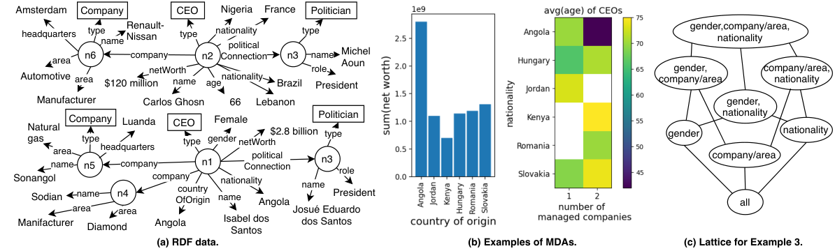
Running examples. Consider an RDF graph comprising politicians, CEOs, and connections between them. We can extract such a graph, for instance, from the WikiData open-source RDF repository. Figure 1(a) shows an example RDF graph where CEOs are linked with politicians, e.g., Isabel dos Santos, a wealthy Angolan CEO (at the heart of the Luanda Leaks scandal), is the daughter of a former president of Angola. Starting from the graph, we aim to automatically identify a small set of aggregate queries that are statistically interesting. Here, interestingness is a statistical measure that indicates deviation from the prior knowledge of the journalists. For example, the interesting aggregate results may deviate from a uniform distribution of values over different aggregate groups, or a normal distribution over numeric dimensions such as age.
Table 1 shows three example aggregates, whose dimensions and measures are either properties in the RDF graph or properties that we derive to enrich the scope of the analysis. In Example 1, CEOs, politicalConnections, countryOfOrigin, and netWorth are either types or properties in the RDF graph in Figure 1(a). Example 2 analyzes the CEOs along the number of managed companies, which is not a property in the graph: we derive it by counting the properties of each CEO. This enables us to discover, e.g., that the average age of Angolan CEOs that manage two companies is low compared to other nationalities. Example 3 analyzes CEOs by areas of companies; we derive this from the graph by following a path from the CEOs to the companies they manage, then to their areas. Similar path examples include company/headquarters, politicalConnection/role; longer paths produce a larger number of novel angles for the analysis.
Among all possible aggregate queries that we can generate, the above three examples are selected because their results show significant deviation from uniform values (having outliers). For Examples 1 and 2, Figure 1(b) shows respectively a histogram that exhibits an outlier in (netWorth) for Angola, and a heat map where the dark color reflects a low value of (age) of CEOs, both due to Dos Santos. We can show to the user such interesting insights as () histograms (if one-dimensional), () heat maps (if two-dimensional), or () tables (for high-dimensional aggregates).
| Example 1 | Sum of the net worth of CEOs with political connections grouped by country of origin. |
| Example 2 | Average age of CEOs grouped by nationality and number of managed companies. |
| Example 3 | Number of CEOs grouped by nationality, gender, and area of the companies they manage. |
Our goal to discover the most interesting aggregates from an RDF graph poses two unique challenges:
Challenge C1 - Aggregate identification. Automatic extraction of interesting aggregates is one among many existing techniques for data exploration and visualization recommendation. Yet, most prior works assume a fixed relational schema (Tang et al. 2017; Vartak et al. 2015). In contrast, in RDF graphs, facts, dimensions, and measures are not specified but must be identified therein. To address this challenge, given an RDF graph, we provide a variety of strategies to create new dimensions and measures, which enable us to examine a rich space of candidate aggregates and to discover the most interesting ones. We further develop a modular framework for aggregate identification, which can be extended or customized as needs arise.
Challenge C2 - Efficient and correct aggregate evaluation. Since we define interestingness on an aggregate result, we must evaluate candidate aggregates to determine if they are among the most interesting ones. A key feature of our work is that we look for multidimensional aggregates (MDAs), such as Examples 2 and 3. A set of dimensions, among which we enumerate candidate aggregates, leads to a lattice (Harinarayan et al. 1996) of nodes, each of which is an MDA (see Figure 1(c)). We may have many such lattices to consider at once, and efficiently evaluating them all poses a salient challenge.
To address the challenge, first, we revisit a classical framework for lattice-based MDA computation in relational data warehouses (DWs). Efficient algorithms, such as ArrayCube (Zhao et al. 1997), compute an aggregate in the lattice from the result of one of its parents, and compute all aggregates in the lattice in a single pass over the data. However, a crucial observation we make in this work is that the classical one-pass approach to lattice computation is incorrect for RDF data, due to a phenomenon called multi-valued dimensions, that is, an RDF node (fact) may have multiple values along a given dimension. To tackle the issue, while retaining the benefits of one-pass algorithms, we provide a theoretical analysis of how the classical approach produces errors. Furthermore, we develop a new RDF-compatible one-pass algorithm that () correctly and efficiently handles lattice-based MDA computation where the aggregates use multi-valued dimensions; () for each node in the lattice (with a given set of dimensions), simultaneously handles many aggregates that differ in the measure (among many possible ones) and the aggregate function in use; () saves computation cost by sharing measures across all lattices that analyze the same set of facts.
Second, to further improve efficiency, we develop a new technique to stop the evaluation of an MDA as soon as we can determine (with high probability) that it will not be among the top . Our technique builds on the work in (Hellerstein et al. 1997), which provides confidence-interval (CI) bounds on an approximate aggregate result. Our problem is harder because we want to approximate the interestingness score computed over the aggregate result, which amounts to estimating the result of a nested aggregate query, whereas the prior work does not support such nested queries. Using advanced statistical tools, we construct CIs for the interestingness function including variance, skewness, and kurtosis over estimated results of candidate aggregates, enabling early pruning of uninteresting aggregates.
In summary, the contributions we make in this work include:
Spade, a new RDF-oriented end-to-end framework that automatically identifies, enumerates, and efficiently evaluates RDF MDAs to determine the most interesting ones (Section 3);
MVDCube, the first correct and efficient algorithm for one-pass lattice-based computation of RDF MDAs (Section 4);
A novel early-stop technique that stops the evaluation of MDAs that, with a high probability, will not be in the top- list (Section 5);
Experimental results validating () the ability of Spade to extract insights from a large space of candidate aggregates; () the frequent, and potentially high errors that existing algorithms introduce on real-life, heterogeneous RDF graphs; () the efficiency of our one-pass algorithm, which is faster than PostgreSQL’s GROUP BY CUBE implementation by 20% to 80%; () the extra speedup of 10% to 43% achieved by our early-stop technique, and () the scalability of Spade as the size and complexity of the graphs increase (Section 6).
2. Problem statement and notation
We consider RDF data defined over three pairwise disjoint sets: the set of URIs , the set of literals , and the set of blank nodes . An RDF graph is a finite set of triples of the form , called subject, property, and object, such that , , and . The RDF property rdf:type is used to attach types to an RDF node, which may have zero, one or several types. Such an RDF graph may have an ontology stating relationships among its types and properties, e.g., any CEO is a BusinessPerson. An ontology leads to implicit triples that together with the triples explicitly present in are the graph’s semantics. All the implicit triples can be materialized via saturation, iteratively deriving new ones from and the rules; we consider ontologies for which this process is finite as in (Goasdoué et al. 2013), and apply it prior to our analysis.
A candidate fact set (CFS) is a set of RDF nodes that we build an aggregate on; we call a member of the set a candidate fact (CF).
An attribute is either a (direct) property (P) of a CF in the original RDF data, or a derived property (DP), which we create from the data and attach to a CF to enrich the analysis. For instance, one may attach to each CEO the number of companies they manage (the full set of derivation strategies is discussed in Section 3). An attribute can be used as a dimension, to group CFs by value, or as a measure, to be aggregated within each group of CFs.
We employ an aggregate function, , that ranges over the common set .
A multidimensional aggregate (MDA), , is determined by: a CFS, a set of dimensions (which are attributes), a measure (also an attribute), and an aggregate function . The semantics of is that of a SPARQL 1.1 aggregate query (Consortium 2013), which also agrees with that of the RDF analytical queries introduced in (Azirani et al. 2015; Colazzo et al. 2014). The result of on an RDF graph , denoted , is the set of tuples, one per each distinct combination of dimension values (aggregate group) in the data:
where has (at least) the values along the dimensions , and iterates over the set of values of the measure on . Finally, is the result of running the aggregate function over the measure values from a given set.
Our semantics, unlike that of relational DWs, does account for heterogeneity in RDF data: () Some CFs may miss dimensions and/or measures, and thus they do not contribute to the result. For the graph in Figure 1, the result for Example 1 is {(Angola, $2.8B)}, due to , whereas does not contribute to the result as it lacks the countryOfOrigin dimension; () A CF may contribute to multiple groups in (if it has multiple values for a dimension), and/or multiple times to the aggregated value (if it has several values for the measure). The result for Example 2 is {(Nigeria, 1, 65), (France, 1, 65), (Lebanon, 1, 65), (Brazil, 1, 65)}, all obtained from given its four distinct values of nationality. Although has both dimensions, it does not contribute to the result as it misses the age measure.
An interestingness function, , is applied over the result of an aggregate . Let be the number of tuples in and, for each tuple , let be the aggregated value computed by . Then takes the set and returns a score, i.e., a positive real number, reflecting a measure of interestingness of . The user chooses the function to be used during the analysis.
Finally, the problem we address is stated as follows:
Problem 1.
Given an RDF graph , a positive integer , and an interestingness function of choice, find the aggregates whose interestingness on is the highest.
3. Overview of the approach
In this section, we describe the system design of Spade, a new RDF-oriented end-to-end framework that automatically identifies, enumerates, and efficiently evaluates MDAs to determine the most interesting ones. Figure 2 shows Spade’s analytics pipeline; it comprises an offline phase, where an RDF graph is loaded and pre-processed, and an online phase, where user-specific analysis is performed.
Offline Processing. Upon loading an RDF graph, we first build a structural summary thereof, using the open-source RDFQuotient tool (Goasdoué et al. 2020). The summary captures all the properties occurring in the graph and proposes a set of RDF node groups such that the RDF nodes in each group are considered equivalent. Spade uses the summary to expedite several steps of the analysis, e.g., the enumeration of RDF types and properties, as described below.
Next, we perform Offline Attribute Analysis with three main purposes: () to gather a set of statistics for each property in the graph, () to determine if derivations should be generated for a given property, and () to decide if pre-aggregated values of some properties should be computed and stored in the database.
Derived properties are the key to a rich search space and to effectively addressing challenge C1. With this aim, we compute statistics including the type of property values (e.g., String, Integer, Date) and, if they are multi-valued, their number of distinct values, the lowest and highest values, etc. Based on these results, Derived Property Enumeration generates: () property counts for multi-valued properties, e.g., how many companies a CEO manages; () keywords occurring in property values, e.g., if a company’s description is “Sonangol oversees petroleum production”, we attach to the company the multi-valued attribute kwInDescription with the values “Petroleum” and “Production”; () the language of a text property, e.g., a company may gain the attribute langOfDescription with the value “English”; () paths, e.g., a CEO politically connected to a “President” gains the attribute politicalConnection/role with the value “President”. Finally, each derived property is also analyzed and stored along with its statistics in the database.
In addition, for each multi-valued attribute, we create a table in the database storing its values, pre-aggregated on the RDF nodes that have it. More specifically, for each RDF node, we compute and store the aggregated value for each (attribute, aggregate function) pair, e.g., the sum of , the count of , the minimum of . This allows Spade to account for facts with multiple measure values and improve Aggregate Evaluation during Online Processing.
Online Processing. The analysis of RDF graphs suits the specific needs of users and proceeds in the following steps.
Step 1 is Candidate Fact Set Selection. To address challenge C1, Spade identifies CFSs in three ways: () type-based: for each type in the graph, the set of RDF nodes of type ; () property-based: for a (user-specified) set of properties, all the RDF nodes having those outgoing properties; () summary-based: each set of RDF nodes identified as equivalent by the RDFQuotient summary; RDF nodes in the same equivalence class tend to have many common properties, making them interesting candidates to be analyzed together.
Step 2 is Online Attribute Analysis. In this step, for each CFS, we first enumerate all direct and derived properties. Then, we enrich the offline-analysis results by adding CFS-dependent statistics, e.g., the support of an attribute among all the facts in the CFS, the number of CFs that have such an attribute more than once, and the number of distinct values. Spade exploits the gathered statistics in different steps, e.g., to guide the choice of dimensions, measures, and aggregate functions and to improve Aggregate Evaluation.
Step 3 is Aggregate Enumeration. Spade uses the pool of analyzed attributes to generate candidate MDAs. To address challenge C1, we generate a rich space of candidate aggregates while applying rule-based pruning to avoid meaningless candidates.
() Identifying dimensions and measures from (derived) properties: We first enumerate all the (derived) properties and consider them for dimensions or measures, subject to the following rules: () Dimensions and measures must be frequent, i.e., having a support greater than a defined threshold; () Dimensions should not have too many distinct values when compared to the number of facts to examine (e.g., we do not consider counting the number of CEOs by their birthday as there are too many distinct values).
() Identifying the dimension set of each lattice: We compute the Maximal Frequent Sets of attributes (Gouda and Zaki 2001) in the CFS. Each of the found sets is the root of one lattice. We further filter them so that each lattice: () has at most attributes, and () does not contain attributes that are derived one from the other, e.g., nationality and numOfNationalities are not allowed as dimensions of the same lattice. Although we aim to offer a general approach, we also note that the readability of MDAs by human users is maximized at levels of relatively low dimensionality, i.e., .
() Identifying the measures in each lattice: Once a lattice acquires dimensions , we assign it a measure set that comprises all the analyzed attributes of the CFS except those in , and those that are derived from a dimension in , e.g., numOfNationalities cannot be a measure in an aggregate whose dimension is nationality.
Several lattices may be found for a CFS, e.g., for CEOs, we have three: {countryOfOrigin}, {nationality, numOfCompanies, and {nationality, gender, company/area (Examples 1-3). They might partially overlap in dimensions and/or measures; e.g., Examples 2 and 3 share nationality. Spade ensures that the results of evaluated MDAs are reused (not recomputed) in the other lattices where they appear.
Step 4 is Aggregate Evaluation. This step triggers the actual evaluation of the enumerated MDAs. To address challenge C2, we combine: () our novel early-stop technique to quickly prune the unpromising MDAs, and () our MVDCube algorithm to efficiently compute the remaining MDAs in a single pass. The final results are produced in an incremental fashion and handled by the Aggregate Result Manager (ARM). The ARM stores them and incrementally updates statistics such as minimum and maximum values, as we explain in Section 4. These are used to determine the interestingness of the computed MDAs (by applying ) in one pass over their results.
Step 5 finally performs Top- Computation. Once the evaluation is complete, the ARM retrieves all the evaluated MDAs, computes their interestingness score by applying , and returns the best aggregates. Spade natively supports three interestingness functions, from which the user can choose to suit their preferences: () variance, () skewness, and () kurtosis, where variance can detect deviation from uniform aggregate values, whereas the latter two can detect deviation from a normal distribution of aggregated values over numeric dimensions. Figure 1(b) shows two example aggregates with high variance scores. More sophisticated interestingness functions for insight detection can be applied on the Step 4 results via the ARM; we discuss early-stop extensions in Section 5.2.
4. Lattice-based computation
We first recall a classical optimized method of computing all aggregates in a lattice. We then explain its limitations and the errors it makes in our setting. Finally, we present our new algorithm to compute lattices of RDF aggregates correctly and efficiently.
4.1. Classical one-pass lattice computation
In relational DWs, nodes in a multidimensional lattice are often computed from one of their parents to reuse computation and limit the number of passes over the data. Among the existing algorithms (Morfonios et al. 2007), ArrayCube (Zhao et al. 1997) computes the whole lattice in a single pass. Given a set of dimensions, a measure, and an aggregate function, it relies on an array representation of data and evaluates nodes through a Minimum Memory Spanning Tree, as we recall below.
Array representation of data. The distinct values of each dimension are ordered, leading to a set of cells, each corresponding to a unique combination of indices of values along the dimensions (axes). In Example 3, assuming nationality {A, B, F, L, N}, gender {F, M} and company/area {A, D, M, N} (we denote initials of the respective values in Figure 3), the multidimensional space has 40 cells, e.g., in cell 0, nationality=A, gender=F and company/area=A; in cell 1, nationality=B, gender=F and company/area=A. Each cell of the -dimensional array contains the value of the aggregated measure over all facts in that cell; in Example 3, this is the count of CEOs. Further, cells are grouped in partitions: each partition is a contiguous part of the array, containing the cells corresponding to a predefined number of distinct values along each dimension, e.g., if this is 2, the 40-cell array has 6 partitions. Figure 3(a) shows the array. Note that an initial pass over the data is required to bring it from the relational to the array representation.
Minimum Memory Spanning Tree (MMST). The dimensions in Example 3 determine the lattice in Figure 3(b). To evaluate all nodes, ArrayCube chooses, for each non-root node , a parent node to compute from, hence forming a spanning tree of the lattice. The memory needed to evaluate all the aggregates in one pass over the data depends on the ordering of dimensions, their numbers of distinct values, and the partition size. ArrayCube chooses the tree that minimizes the overall memory needed; it is called the MMST.
Lattice computation proceeds as follows. The MMST is instantiated, allocating to each node the required memory. Partitions are loaded from the array representation of data, one at a time, into the root of the MMST. The content of each cell in the root is propagated to the children and used to incrementally update the aggregated measures of all the nodes in the MMST. Once a partition is evaluated, each node checks if it is time to store its memory content to disk. For instance, after scanning partition P1 in Figure 3(a), the subarray with nationality {A, B} and company/area {A, D} is exhausted. Thus, the counts of CEOs with either of the two nationalities, and A or D company area are computed. Now, (Figure 3(b)) can store its result to disk and reuse the memory in the subsequent computation. Similarly, once processed, the two subarrays of P2, () nationality {A, B}, and company/area {M, N}; () nationality {A, B}, are exhausted, and both and can store their results to disk. stores its result after every partition, after every two.
4.2. Incorrectness in the RDF setting
Results computed by ArrayCube may be incorrect in the presence of multi-valued dimensions. Consider our running examples that show CEOs with various nationalities and at most one gender who manage companies in several areas. In a relational DW, each such CEO would be stored as a tuple in the fact table, and their multiple nationalities (respectively, company areas) would be modeled as a dimension table associating them with each of their nationalities (company areas). We could then find the result for Example 3 with a query that joins all the relations, groups the data by the dimensions, and finally aggregates the measure. To evaluate all MDAs in the lattice determined by the dimensions, ArrayCube would use the MMST in Figure 3(b) and compute the aggregate by means of , using its result to compute the rest of the lattice.
Figure 4 shows the result of when applied to the two CEOs in Figure 1. The tuples to are derived from Dos Santos (the RDF node ), whereas to are due to Carlos Ghosn (the RDF node ). Since lacks gender information, the tuples to have gender=null. We need to keep them to compute the rest of the lattice correctly. Since has valid values for nationality and company/area, we must count this CEO when computing aggregates over one or both of these dimensions, e.g., in Figure 4. We obtain the result of by aggregating ’s result to project away the nationality dimension. For instance, the tuples , , , and , which are all associated with , collapse into the tuple in where now this CEO counts as four. Then, is further aggregated by projecting away company/area to compute and separately gender to compute . The cardinality “bug” introduced in propagates down the lattice. In ’s result, we find five CEOs managing Manufacturer companies, whereas there are only two. A similar error occurs in where we count three female CEOs because the tuples to of are aggregated into the same tuple and are, thus, counted three times (although they all represent ).
The above example shows that multiple values for a dimension may lead to errors when an aggregate is computed from one of its parents. To correctly compute the whole lattice from the root aggregate, naïve solutions may: () require that each CEO fact be represented by at most one tuple, e.g., in our example, by ignoring all but one of Ghosn’s nationalities (company areas); this would clearly miss an interesting part of the data; () compute each of the aggregates in the lattice separately, missing the benefits of efficient one-pass algorithms; this would entail a high run time overhead.
Interestingly, if we alter the query to count distinct CEOs in each group (in lieu of ), no errors occur in the result of Example 3. By design, ArrayCube cannot compute aggregates including distinct: instead, it computes all aggregates from the result of the lattice root, where information about individual facts is no longer present. Other one-pass algorithms for lattice-based aggregate computation, such as PostgreSQL’s GROUP BY CUBE implementation (Group 2020) (PGCube), do support the counting of distinct values and can thus be used to obtain the correct result for Example 3. However, in the presence of multi-valued dimensions, computing aggregates from the result of one of their parents in the lattice may still lead to wrong results, as illustrated in the following variations of Example 3.
Variation 1. Consider the aggregate “sum of the net worth of CEOs by nationality, gender, and area of the companies they manage”. We first augment the data in the root aggregate with the sum of netWorth (). The tuples to contain the of Dos Santos: $2.8 billion. The tuples to contain the of Ghosn: $120 million. We then compute the sum of by company/area. The tuples , , , , and (all having company/area=M) sum up into one tuple, and result in the sums of $2.8B of Dos Santos, and $120M of Ghosn, whereas both CEOs should have contributed exactly once. Moreover, we cannot solve this issue with the (distinct NW) aggregate. If both CEOs had the same , a (distinct) would sum once, instead of (correctly) summing it twice.
Similarly, the following variation illustrates another scenario leading to wrong results.
Variation 2. Consider the aggregate “average age of CEOs by nationality, gender, and area of the companies they manage”. We obtain it as (age)/(age), i.e., the sum in Variation 1 is divided by 5. Instead, the correct value is sum of ages of Dos Santos and Ghosn divided by 2. As in Variation 1, we cannot solve this issue by using (distinct age).
As our experiments show (Section 6.3), the number of incorrectly computed aggregates, and the magnitude of the error itself, can be quite significant. This is because of the flexible RDF model, which allows multi-valued dimensions. Conversely, in a relational DW, once a fact table is joined with dimension tables, ArrayCube assumes that each fact has exactly one value for a dimension (for instance, due to a functional dependency). Below, we formally characterize the situations when ArrayCube introduces errors on RDF data.
Analysis of ArrayCube errors on RDF. Consider an RDF graph and a lattice of dimensions ( nodes) on . Whether a lattice node can be computed correctly from one of its parents, depends on the presence of multi-valued dimensions in the lattice:
Lemma 0.
Let be an RDF graph. Let , be two aggregates in a lattice on such that is a parent of , where is a dimension, , and there exists a fact with more than one value along the dimension . Then, computing from the result of may lead to wrong results.
Proof.
Let the fact have the values and, for each , , and is not null. By definition of , there exist tuples such that and , to both of which contributes. Hence, there exists a tuple such that , in which the dimension does not appear.
When computing from , the aggregated value is obtained from and based on the function . For instance, if is , the fact will be counted twice, instead of just once. If is , the value(s) of will be summed twice, which falsifies the result (except for the particular case where their sum is 0). Computing the may similarly lead to wrong results. ∎
How does Lemma 1 impact the one-pass lattice-based computation for a given graph ? We show the following result:
Theorem 2.
Given an RDF graph and a lattice on , let be the set of all the dimensions for which some fact(s) have more than one value, and let be the size of . () A one-pass algorithm cannot compute correctly all the lattice aggregates. () The maximum number of MDAs (lattice nodes) that can be computed correctly (depending on the choice of the MMST) is .
Proof.
() Among the lattice edges, are labeled with a dimension from , meaning that the dimension is projected away when computation follows this edge. As Lemma 1 shows, if the MMST contains one such edge, the result of the child node of that edge may contain errors. However, no spanning tree, thus, no MMST, can avoid all edges labeled with a dimension in . This is because to go from the root, whose dimensions are , to a node lacking one dimension , by the construction of the lattice, the MMST must traverse an edge labeled .
() The lattice nodes that can be computed correctly in one pass (starting from the root’s result) are exactly those having all the dimensions: a node lacking one such dimension would be obtained by aggregating a parent’s result along that dimension, and thus, by Lemma 1, be wrongly computed. The lattice has such nodes. Fewer nodes may be computed correctly if the MMST picks a “wrong” edge, even if it could have avoided doing so. ∎
4.3. MVDCube Algorithm
We now present Multi-Valued Data Cube (MVDCube), our new one-pass MDA evaluation method. Going beyond existing algorithms (Zhao et al. 1997), MVDCube: () produces correct results even in the presence of missing or multi-valued dimensions and/or measures, () computes several aggregate functions over a large set of measures in the same lattice, and () saves computation cost by sharing measures across all lattices from a given CFS.

Before we move forward, we clarify that our RDF database uses the following storage: a CFS is represented by a single-column table storing the identifiers (IDs) of the facts; for each attribute , a table stores (, ) pairs for each triple in the RDF graph.
Figure 5 depicts the main features of MVDCube. Our MVDCube evaluation method proceeds in the following steps, with the pseudo-code of its core functions shown in Algorithm 1.
Building MMSTs. Given a CFS and a set of lattices (identified in Step 3 of Spade’s pipeline), each with the dimensions and the measures , we construct one MMST per lattice as in (Zhao et al. 1997).
Data Translation. For each lattice, we process the root node by sending a join query to the database to obtain all the CFs that have a value for at least one of the dimensions in . We then translate the join result to lay the data in a partitioned array representation of cells. A partition is a set of pairs (cell index, CF). We assign each RDF node a cell index based on its dimensions’ values; in the case of multiple values for a dimension, we assign indexes of all corresponding cells. We add the special value null in the domain of each dimension to account for missing values. Therefore, each cell is associated with the set of RDF nodes that correspond to the combination of dimension values that this cell represents. Like ArrayCube, we take an initial pass over the data to bring it into the array representation, where the (conceptual) multidimensional array is stored as a serialized one-dimensional array. If the data does not fit into the available memory, we partition it, store to disk, and later read back, one partition at a time; otherwise, MVDCube accesses the array directly from the main memory, in a single pass, in subsequent steps.
Measure Loading is performed in parallel to the Data Translation step. For each measure in , we query the database to retrieve, for each CF, the pre-aggregated values of (which were computed and stored offline). We load the values ordered by the IDs of the CFs, and share them among all MMSTs in a given CFS. As they are stored at the granularity of a CF, they can be used to compute aggregate results for all cells, as we describe below.
Lattice Computation is then carried out in one pass over the data using the MMST. MVDCube associates an MMST node with a (large) set of aggregates; we denote such a node as . Each node then represents all the MDAs that have dimensions (but might differ in their measure and aggregate function). Suppose that we want to compute the lattice with ={gender, company/area, nationality}, ={age, netWorth} and that age is associated with , and netWorth is associated with . Node in Figure 5 represents the two MDAs: () average age of CEOs, and () sum of netWorth of CEOs, both grouped by gender and company/area.
In the MMST, we allocate, for each node, the needed memory. We load partitions successively into the root. In Figure 5, we assume that each partition contains 3 distinct values of each dimension, hence 27 cells. For compactness, we encode each set of RDF nodes in a cell using a Roaring Bitmap (Lemire et al. 2016) (also adopted in Spark because of the strong compression and lookup performance). In Figure 5, each cell stores a set of CEOs (a subset of the facts and ). The bitmaps follow the same ordering of the CFs applied during Measure Loading. The cell of index 3 in contains a bitmap of size 2, BM, representing that is in the set, whereas is not.
(a) Projection and bitmap propagation. We scan the bitmaps in the cells of the root node and immediately propagate them to the child nodes in the MMST as dimensions are projected away (line 1 in Algorithm 1). We union (OR) the bitmap in each cell in a child node with each bitmap received from the parent (line 1): this models the contribution of all facts in a parent node to the corresponding cell in the child node. In particular, as we project away a multi-valued dimension from a parent node to a child node, if a fact has multiple values of the dimension, it belongs to different cells in the parent node, but will be consolidated in the same cell in the child node.
Red arrows in Figure 5 show propagations. For example, the bitmap of cell 2 in node , BM2, is initially empty (i.e., 00). Then it is updated to 01 when BM8 from is propagated, and later to 11 when BM2 from is also propagated.
Once a partition is evaluated, we apply the ArrayCube check (Section 4.1) in the nodes to learn if it is time to write results to disk (line 1). If so, we first propagate their memory content to their child nodes (line 1), and then we compute the values of the aggregated measures and store them (line 1).
(b) Measure computation (denoted as ). When a node is ready to write to disk, we scan its memory one cell at a time. For each cell: () we identify the pre-aggregated measures of each RDF node in the cell’s bitmap, and () we apply the relevant aggregate functions to them. Note that measure computation is very fast as both the bitmaps and the pre-aggregated measures are ordered by the fact ID, and can aggregate different measures simultaneously.
Revisit in Figure 5. Once P1 and P2 are evaluated, is ready to write current results to disk. We scan the three cell bitmaps, and for each bitmap: () identify the age and the net worth of each CEO in the bitmap by accessing the pre-aggregated measures, () aggregate the respective measures by applying on the age and on the net worth. For example, for BM2, we identify the ages (respectively, net worth) of : 47 ($2.8B) and : 66 ($120M) because they are both present in the bitmap, then compute their average (respectively, sum). The Aggregate Result Manager (line 1) receives the computed measures, and the values of the dimensions obtained from the cell index. Finally, we empty ’s memory in the MMST and reuse it to evaluate the aggregate on the next partition (line 1).
Memory usage. Our memory analysis builds on the corresponding ArrayCube study (Zhao et al. 1997). Assuming dimensions with distinct values each and distinct values per partition, the MMST uses at most array cells to compute one aggregated measure. In MVDCube, the memory for an MMST is also upper bounded by cells. However, cells have a variable size as each of them contains a Roaring Bitmap (RB). For this reason, we provide a worst-case estimation of MVDCube’s memory needs for the MMST and the pre-aggregated measures.
() The size of an RB used to store integers in the interval is bound in (Lemire et al. 2016) to , that is, beyond a fixed overhead for , the universe size, RBs never use more than 2 bytes per integer. In the worst case, we could have facts in each cell, occupying a total of bytes.
() For measures, MVDCube needs float numbers in the worst case, where refers to each measure and is the set of aggregate functions assigned to the measure. As an optimization, we detect, offline, the numeric properties having at most one value for all their RDF nodes, e.g., the age of CEOs. To save memory, we allocate a single float number for all pre-aggregated results (, , and ) for such properties.
5. Early-stop aggregate pruning
To reduce the effort required to compute lattices of aggregates, we have developed a novel technique called early-stop (ES).
5.1. The early-stop principle
Given an aggregate and an interestingness function , finding, how interesting is, amounts to evaluating a query of the form:
| SELECT (aggregated) FROM |
| (SELECT AS aggregated |
| FROM GROUP BY ) AS inner; |
where is joined with dimensions and the (pre-aggregated) measure . Note that we only need to present the result of the inner query to the user, if ends up in the top-. This leads to the following idea: we could reduce the effort to compute some aggregates if we can determine (with high probability) that they will not be among the most interesting ones.
The literature (Hellerstein et al. 1997; Haas 1997) introduced conservative and large-sample confidence intervals as means of estimating the result of a query such as inner but not the result of the full nested query, i.e., the interestingness score that we aim to obtain. Recent work on visualization recommendation (Vartak et al. 2015) shows how to stop the evaluation of low-utility one-dimensional aggregates early on relational data. In doing so, it relies on a worst-case (conservative) confidence-interval-based pruning. In contrast, we extend the line of research on aggregate pruning by constructing a large-sample confidence interval around the interestingness score estimator. We provide our novel approach and formalize its probabilistic guarantees below.
To enable early-stop pruning, we estimate the interestingness of the aggregate using an estimator , and bound this approximate score within our large-sample confidence interval. (We derive the formula for the interval in Section 5.2.) We draw from each aggregate group a sample containing the same number of facts. For the sake of efficiency, our sampling procedure proceeds in batches of a given size. After scanning a batch, we update the estimate of the aggregate’s interestingness based on the (pre-aggregated) measure values of the facts in the batch. To prune some aggregates, if we find that the upper-bound on the estimate of ’s interestingness is lower than the current lower-bound of the -th best aggregate, we can give up evaluating , and thus obtain the top- aggregates more quickly. The central part of Figure 5 illustrates this with five aggregates and : the fifth aggregate can be stopped after the current batch, whereas the estimation of the fourth aggregate will continue in the next batch. This procedure terminates once the sample is exhausted or no aggregates have been pruned in a given number of batches.
5.2. Estimating the interestingness score
Notation recall. A simple random sample of size is a vector of values drawn uniformly without replacement from a population of size ; the sample is modeled by a set of independent, identically distributed (i.i.d.) random variables .
An estimator is a random variable equal to a linear or nonlinear combination of (typically modeling a simple random sample). Evaluating the estimator on a vector of concrete values taken by these random variables yields an estimation.
Let be a statistic of , be an estimator of the true value of based on a sample of size , and be a confidence level for . Then, a -confidence interval (CI) is a random interval such that for each , . One interval is derived deterministically from one sample; the probability is taken over all such intervals. We denote and , respectively, the lower and the upper bounds at confidence level on . As in (Hellerstein et al. 1997), the large-sample confidence interval contains the true value with the probability approximately equal to .
Constructing the estimator. We begin by developing formulas for the point estimator of the query’s result when the aggregate function () in use is , , or and the interestingness function () is variance, skewness, or kurtosis. We first detail this for , and variance and then discuss extensions to other functions.
Let be the aggregate groups of and be the true result of , that is, the vector containing, for each group, the average of the pre-aggregated values of for facts from that group. Further, for each group , let be the sample mean estimator, where the variable has mean and variance and models the (pre-aggregated) measure value of the -th fact of the sample of size , drawn from the facts in . Note that, from the Central Limit Theorem (Theorem 5.5.14 in (Casella and Berger 2001)), each as , where is the normal distribution centered in with standard error .
We estimate with , where is the vector of all the group estimators. We thus obtain the (unbiased) estimator of the variance of a vector :
| (1) |
Deriving CI bounds. We aim at providing a large-sample confidence interval around . Our formal result is as follows:
Theorem 1.
Let be the estimator of variance. There exists an error such that with the probability approximately equal to .
Proof.
We prove Theorem 1 constructively, thus exhibiting a concrete formula for . To derive the confidence interval, first, we approximate around using the first two terms of its Taylor series expansion: . Then, we apply the Multivariate Delta Method (Theorem 5.5.28 in (Casella and Berger 2001)) to state that
| (2) |
where denotes convergence in distribution, , for . In other words, the difference between the correct value of interestingness, , and that on the estimator, , converges in distribution to a -centered normal distribution.
To apply this theorem, we must show that (1) has continuous first partial derivatives and that (2) . Condition (1) can be easily shown by applying basic calculus on Eq. 1. For (2), we assume that are independent random variables. Hence, for , if , then , else , and is positive.
We now move toward a formula for the confidence interval based on the samples in the groups. We derive it by “standardizing” the distribution of the difference obtained in Eq. 2, and taking quantiles of the standard normal distribution, , as the interval’s ends.
Let , where are (unbiased) estimators of variances in all the groups. From the Strong Law of Large Numbers (Theorem 5.5.9 in (Casella and Berger 2001)), we have that almost surely. Then, applying Slutsky’s theorem (Theorem 5.5.17 in (Casella and Berger 2001)), we get . In turn, for large , we obtain: , where denotes the cumulative distribution function of a normally distributed variable.
Let be the quantile of . Solving for , gives us . Finally, choosing we obtain the approximation at the desired confidence level:
∎
Other interestingness functions. To derive confidence intervals for skewness and kurtosis, we follow similar derivations by replacing the definition of (Eq. 1) with their respective formulas. We derive the CIs based on the Delta Method – both cases exhibit continuous first partial derivatives; see Appendix A. In general, one can derive similar formulas for any interestingness function that meets conditions (1) and (2).
Other aggregate functions. For , we estimate the group sizes while sampling and compute the estimate as a product of the and estimates. For and , we use the sample min and the sample max, respectively, as point estimates; we apply Popoviciu’s and Szőkefalvi-Nagy’s inequalities (Popoviciu and Szőkefalvi-Nagy 1935) for the upper and lower bounds, respectively. See Appendices B, and C for details.
5.3. Plugging early-stop into MVDCube
We integrate early-stop into MVDCube to speed up Aggregate Evaluation, and thus address challenge C2. The evaluation of an MMST begins with the Data Translation step, run in parallel with Measure Loading (recall Section 4.3). We exploit the data translation to create a stratified sample of facts for the early-stop pruning. Given the MMST, each address in the multidimensional space in the root corresponds to a unique group of facts. We allocate empty reservoirs , one per aggregate group, each with a capacity equal to the sample size: this way we ensure stratification. While reading each tuple, we determine its group, hence also the reservoir, and either put the fact in or not with some probability. If the reservoir is full, we discard one of the previously inserted facts. This strategy is known as reservoir sampling and guarantees a choice of a simple random sample (Vitter 1985). Figure 5 shows an on-going sampling process with four reservoirs to , each of size 3.
The sample thus obtained is used by early-stop as follows. Once the translation is finished, we propagate the facts sampled from the MMST’s root down the tree using Roaring Bitmaps as in MVDCube (see Figure 5): each node in the MMST receives its own sample. Then, we perform the early-stop pruning based on these samples. All the aggregates that have not been pruned (deemed sufficiently interesting) by early-stop are subsequently evaluated by MVDCube.
6. Experimental evaluation
| Dataset | #triples | #CFSs | #P | #A | #DP | #A | |||
|---|---|---|---|---|---|---|---|---|---|
| woD | kw | lang | count | path | wD | ||||
| Airline (Gonzalez 2016) | 56M | 1 | 30 | 5,923 | 0 | 0 | 0 | 0 | 5,923 |
| CEOs (Mazuran 2020) | 85k | 237 | 61 | 159 | 1 | 1 | 37 | 462 | 27,860 |
| DBLP (Fragments 2017) | 33M | 1 | 21 | 1 | 5 | 3 | 8 | 19 | 961 |
| Foodista (Dodds 2011) | 1M | 5 | 13 | 0 | 1 | 1 | 6 | 38 | 14 |
| NASA (Dodds 2010) | 99k | 10 | 37 | 19 | 3 | 15 | 3 | 87 | 1,449 |
| Nobel (Committee 2020) | 87k | 15 | 39 | 58 | 3 | 3 | 18 | 87 | 30,658 |


Computational environment. We ran all experiments on an Intel Xeon CPU E5-2640 v4 @ 2.40GHz, 40 cores (2 sockets with 10 physical cores each, hyper-threading enabled), running CentOS 7 with 90GB for JVM (OpenJDK 1.8) and 30GB for PostgreSQL 12.
Systems. We implemented Spade in Java 1.8 (18k lines of code); it relies on OntoSQL 1.0.12, an efficient RDF storage and query answering platform on top of an RDBMS (Bursztyn et al. 2016; Buron et al. 2019; Buron et al. 2020) (PostgreSQL in our case). We compare the performance of our aggregate evaluation method against the best-effort baseline, which uses PostgreSQL’s GROUP BY CUBE implementation, since 2016 based on an efficient one-pass computation of all aggregates in a lattice (Group 2015), that supports additional features such as (distinct), which were not available in ArrayCube (Zhao et al. 1997). We denote this by PGCube. As discussed in Section 4.2, PGCube may fail to compute correct results in the presence of multi-valued dimensions. However, the support for counting of distinct values may help PGCube correct some wrong results. Thus, we consider two variants: () PGCube computing counts using , denoted PGCube∗, and () PGCube computing counts using (distinct), denoted PGCubed. In both cases, our Java code is at a disadvantage against a C/C++ engine.
Real-world graphs. Our experiments involve a set of real-application RDF graphs, for which Table 2 shows: the number of triples, the number of CFSs, the number of (direct) properties and derived properties (#P and #DP, respectively) in the graph, and the number of aggregates without and with derivations (#AwoD and #AwD, respectively). The graph sizes in this work are similar to the real-world dataset sizes used in comparable relational works, e.g., 20k tuples in (Tang et al. 2017), and up to 60M tuples in (Vartak et al. 2015). Airline was originally a relational dataset on flight delays used in prior work (Vartak et al. 2015); we converted it into RDF (each tuple becomes a CF with a fixed set of properties), whereas the others are natively RDF. We discuss differences between this and the other graphs shortly.

6.1. Analysis of example results
We begin by showing, in Figure 6, example interesting aggregates found by Spade when using variance as an interestingness score:
() “Minimum net worth of CEOs by gender and occupation”: () there are two outliers, male philanthropists and male shareholders: their minimum net worth is much higher than others’; () the net worth value is known for all but one occupation for male CEOs, but only in a half of them for female CEOs; () the minimum net worth of female CEOs is nearly the same across occupations.
() “Number of launches by launch site and spacecraft/agency” in the NASA graph: () very high values for USSR spacecrafts launched from Plesetsk and Bajkonur; () the most used USA launch sites are Cape Canaveral and Vandenberg Base. These interesting insights were discovered thanks to our path derivations.
() “Average mass of spacecrafts by discipline”: here 4 disciplines, i.e., Human crew, Microgravity, Life sciences and Repair stand out with the average spacecraft mass significantly higher than others’.
Nonetheless, many candidate MDAs are uninteresting: Figure 8 shows the aggregate “minimum number of occupations of CEOs by gender and number of companies” in the CEOs dataset, where all aggregated values are uniformly equal to 1; or “average number of launched vehicles by launch site” in the NASA dataset, where most values are equal to 1, and only 8 out of 35 bars are slightly higher but still less than 1.05. These aggregates don’t exhibit any significant outliers and were therefore ranked low by Spade.


This confirms the need for using early-stop to prune such MDAs.
It could have been in principle envisioned to compare the interestingness of the aggregates found by our system with that of some manually chosen aggregates. However, doing so is hampered by the lack of feasible selection methods available to human users. For this reason, the starting point of our work is precisely the observation that it is very hard to select aggregates manually. There are several reasons for this: () The sheer size of the graph impedes human understanding, and it is hard to induce human users to attempt solving such a computationally expensive task at all. Even if they did try to solve it, typically, such users would use a simple SPARQL engine that can evaluate aggregates, and hence they would have to formulate the queries themselves, which requires expertise in writing such complex aggregate queries. () Even if we reduce a graph to a modest size, e.g., through summarization (Liu et al. 2018; Cebiric et al. 2019) or sampling, the reduced graph may not reflect () all possible combinations of facts, dimensions, and measures in the original data; () the graph values, e.g., the frequent values and value distributions; or () any derived properties. Even under strong (unrealistic) assumptions, e.g., () and () are both known for a simple, regular RDF graph, users would still not know which aggregates are interesting (e.g., deviating from a uniform distribution) before enumerating and evaluating them all at least partially. () Supporting interactions with the system leads users inevitably to inject some information about their preferences in the aggregate selection process. For example, in the NASA dataset, the users may prefer to investigate launches grouped by the launch site rather than the discipline of the spacecraft staff. In contrast, Spade is a fully automated approach to discovering statistically interesting aggregates, with no user input required. It defines and enumerates a large set of candidate aggregates by applying heuristics to generate potentially interesting dimensions and measures and evaluates them efficiently.
As examples in Figure 6 show, our highly-ranked results returned from the six real datasets reveal interesting insights. Due to the automatic nature of Spade, in some datasets, there may be a small fraction of aggregates that, despite being statistically sound, are unlikely to be chosen by the user. For example, the aggregate minimum net worth of CEOs by nationality/image uses a derived property, nationality/image, which is statistically similar to other meaningful dimensions, e.g., nationality/label, but the user is unlikely to choose it. This indicates that a “human-in-the-loop” approach can further improve the effectiveness of our automated approach. While for the above example, the user can simply add nationality/image to a stop list for dimensions, a full design of “human-in-the-loop” data exploration will be a focus of our future research.
6.2. The benefits of derived properties
We begin our evaluation by validating the benefits of Derived Property Enumeration (Section 3). This step is crucial to address challenge C1. We show that it allows us to increase the pool of attributes and to generate a large and rich space of interesting aggregates.
Experiment 1. We compare the results of our analytical strategy when: () only RDF graph properties were used for the analysis (woD), and () derived properties were also considered (wD). As Table 2 shows, the Airline dataset (originally relational) leads to no derivations: tuples are not linked to each other, and thus no paths can be derived; it lacks multi-valued attributes, thus no count derivation applies; the data is mostly numeric, so keyword or language attributes are not derived. The other (native RDF) graphs differ drastically: they feature several CFSs, multi-valued properties, links among RDF nodes leading to many path derivations (Table 2 shows counts of path derivations of length 1, as they are the most numerous); textual attributes are also quite frequent. Figure 7 further shows, for each graph, the interestingness of its MDAs (measured with variance) in woD and wD settings (left and right lines, respectively); a horizontal tick in a line depicts an MDA.
Our first main observation, denoted as remark (R1), is that () derivations increase the total number of enumerated MDAs: for instance, on Foodista, no MDA exists without derivations, whereas we find several by deriving the recipe language, the count of ingredients, etc.; on DBLP, only year is a good dimension, whereas through derivations we obtain, e.g., ; () derivations increase the interestingness of the best aggregates.
Henceforth, we enable derivations in our experimental analysis.
6.3. Analysis of MVDCube against PGCube
Our next set of experiments focuses on Aggregate Evaluation, the last step of our online pipeline, where most computation takes place. Since PGCube is not able to prune unpromising aggregates, for fairness, in this section, early-stop is disabled.
Experiment 2. We compare MVDCube with PGCube in run time and quality (correctness). Recall that PGCube’s results may be erroneous (Section 4.2). We use the six real graphs with derivations.

| Dataset | PGCube∗ | PGCubed |
|---|---|---|
| #wrong aggs | #wrong aggs | |
| Airline | 0 | 0 |
| CEOs | 4,723 | 3,998 |
| DBLP | 102 | 87 |
| Foodista | 2 | 0 |
| NASA | 378 | 312 |
| Nobel | 4,154 | 3,821 |
errors on real-graph aggregates.
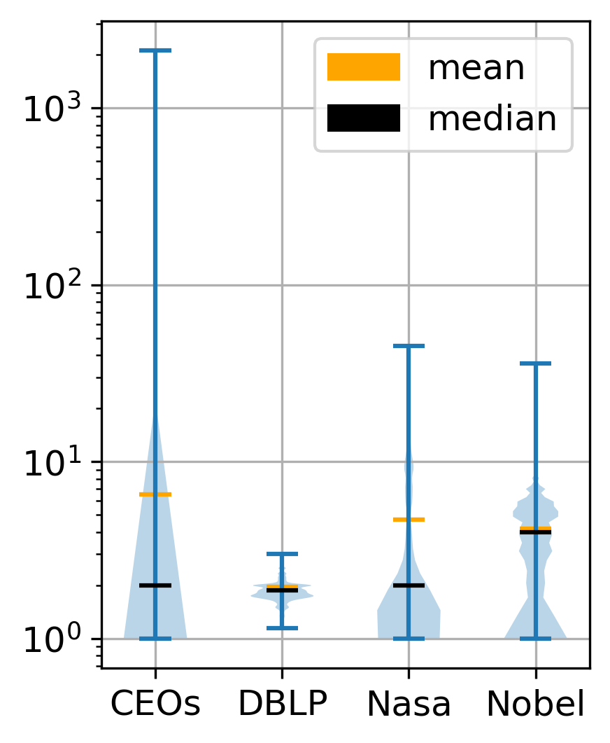
of PGCubed errors.

Regarding the run time, Figure 9 shows MVDCube against PGCube∗ and PGCubed on our real datasets. We observe that MVDCube achieves a time gain of 20% to 80% over PGCube∗ and of 30% to 83% over PGCubed on most datasets (R2). Specifically, MVDCube outperforms PGCube when there are many (more than 15) aggregates to evaluate (R3). This is because MVDCube: () shares measures across all the aggregates from the same CFS, and () computes each aggregate only once, even if it appears in several lattices. In contrast, PGCube evaluates each lattice in a separate query, each of which joins the facts with the measures. Except for the Foodista dataset, which has a small number of aggregates and both methods run under a second, MVDCube shows significant gains on CEOs, NASA and Nobel Prizes graphs, where many MDAs are evaluated, MVDCube gains 40% over PGCube. Similarly, Airline leads to almost 6k MDAs, the dataset is rather large (6M facts), and the repeated joins are expensive: PGCube∗ takes 5 times MVDCube’s time.
Regarding the errors, Table 3 shows, for each graph, the number of aggregates with incorrect results (#wrong aggs) for PGCube∗ and PGCubed. We observe that PGCube∗ and PGCubed produce errors in, respectively, 14% and 12% of all computed aggregates (R4). PGCubed, PGCube’s best effort to generate correct results, still produces errors in 9% to 21% of the computed aggregates across different datasets. As shown in Section 4.2, errors are related to multi-valued attributes in the data. Indeed, CEOs, NASA, and Nobel Prizes datasets have the greatest number of multi-valued attributes and the highest error, ranging from 12% to 21%.
Experiment 3. We now quantify the error in those aggregates that are computed wrongly by PGCubed. Given an aggregate , we denote the value of the aggregated measure of the -th group in , as computed by MVDCube. We denote by the value that PGCubed computes for the same group. As can only be higher than or equal to the correct value , ideally, this ratio should be . When an aggregate is shared by two lattices, it can be computed from either lattice, leading to different error ratios. When this happens, we record the maximum error, to measure the “worst-case risk” incurred by evaluating the lattice through PGCube. Each aggregate thus leads to a set of error ratios, one per group. Figure 10 shows their distribution, for and aggregates, for the four datasets from Table 3 where errors were detected. We note that errors can easily exceed one order of magnitude (R5): in 3 out of 4 cases, PGCubed produces at least 1 tuple whose value is more than 30 times the true value. In CEOs, one group records an error ratio greater than ; it comes from a three-dimensional lattice where all dimensions were multi-valued. Such incorrect values would severely falsify the selection of the most interesting aggregates.
6.4. Impact of early-stop on MVDCube
Experiment 4. We next study the effectiveness of our early-stop technique (ES). For our real graphs, Table 4 shows: () the evaluation time taken by MVDCube alone, () the time with ES enabled, as described in Section 5.3, () the time gain due to ES, () the fraction of aggregates pruned and () the accuracy of ES. Following (Vartak et al. 2015), if and are the sets of the top- aggregates returned by MVDCube without and with ES, the accuracy is computed as the fraction of true positives in : . We show this for , in keeping with comparable works in a relational DW setting (Vartak et al. 2015) and using a sample size of with 2 batches, a configuration we found empirically to work well. Table 4 leads to two observations. First, ES can bring significant evaluation time gains, from 10% to 43% in our experiments; and it aggressively prunes uninteresting aggregates, frequently as much as 70% (R6). ES is especially beneficial on graphs with more than 100 aggregates, except for DBLP, where translating the data into an array representation is much more expensive than evaluation, and thus, the saved evaluation effort appears small. In some cases, the impact of ES was negative (and very small), due to a sampling overhead. Second, MVDCube with ES is often quite accurate (R7): 100% accuracy is attained in the majority of cases, except for Nobel Prizes, where, e.g., the true top- contains aggregates with interestingness score greater than , whereas ES returns those greater than .
| TOP 3 | TOP 5 | TOP 10 | |||||||||||||
|---|---|---|---|---|---|---|---|---|---|---|---|---|---|---|---|
| dataset | MVD | MVD+ES | gain% | pruned% | acc% | MVD | MVD+ES | gain% | pruned% | acc% | MVD | MVD+ES | gain% | pruned% | acc% |
| Airline | 381,710 | 316,168 | 17.17 | 96.13 | 100.00 | 369,369 | 316,885 | 14.21 | 93.52 | 100.00 | 373,660 | 330,467 | 11.56 | 88.10 | 90.00 |
| CEOs | 18,114 | 14,624 | 19.27 | 79.21 | 33.33 | 18,685 | 14,108 | 24.50 | 72.86 | 100.00 | 18,047 | 15,108 | 16.29 | 66.86 | 100.00 |
| DBLP | 256,832 | 255,918 | 0.36 | 88.03 | 100.00 | 250,916 | 248,982 | 0.77 | 85.33 | 100.00 | 249,463 | 256,325 | -2.75 | 80.85 | 100.00 |
| Foodista | 855 | 917 | -7.25 | 0.00 | 100.00 | 1,173 | 893 | 23.87 | 0.00 | 100.00 | 886 | 920 | -3.84 | 0.00 | 100.00 |
| NASA | 8,633 | 7,366 | 14.68 | 82.40 | 100.00 | 8,581 | 7,750 | 9.68 | 76.54 | 80.00 | 8,458 | 8,151 | 3.63 | 59.01 | 100.00 |
| Nobel | 24,633 | 13,897 | 43.58 | 95.94 | 0.00 | 24,453 | 13,829 | 43.45 | 95.59 | 20.00 | 23,848 | 14,267 | 40.18 | 94.70 | 30.00 |
6.5. Scalability study
We finally analyze the scalability of our approach and compare it with PGCube, when varying different data characteristics. To be able to fully control them, we designed a synthetic benchmark (a set of graphs) with fixed numbers of facts , dimensions and measures. All property values are numeric. We ensure that a single CFS is found and that each dimension , , takes at most values (so that they are considered good dimensions, recall Step 2 in Section 3). We denote each graph by : : : , the maximum number of distinct values along each dimension. To obtain realistic distributions of the facts in this multidimensional space, we randomly assign dimension values as in (Agarwal et al. 1996), controlled by a sparsity parameter . To ensure PGCube correctness, each fact has only one value for each dimension.
Experiment 5. We analyze the performance of the entire online pipeline of Spade on benchmark datasets. We use 12 configurations, each having =, 3 dimensions, and 3, 5, or 10 measures. We also use () two different combinations of distinct values for dimensions, 100:100:100 (uniform) and 100:5:2 (decreasing), and () two different sparsity coefficients, and . In Figure 11, each bar represents one configuration (“u” or “d” for value distribution | sparsity coefficient | number of measures) and reports the total execution time of Spade using MVDCube without early-stop. Each segment of a bar covers one computation step (recall Figure 2). In the pipeline order of steps, we observe that: () Candidate Fact Set Selection is too fast to be visible; although there is only one CFS here, in all our experiments with real graphs, it was 5-10 ms. () Online Attribute Analysis’s time is noticeable, between 15% and 37% of the total time, and increases with the number of measures: Spade must analyze them before deciding that they are not suitable dimensions. () Aggregate Evaluation dominates the processing time; it increases with the number of distinct groups and the number of measures as each measure leads to a different aggregate. () The time to select the best aggregates (evaluate their interestingness and pick the top-) is also noticeable and grows as expected with the number of aggregates. () Sparsity has a moderate impact. From these results, we conclude that for a fixed CFS, Aggregate Evaluation dominates Spade’s execution, increasing with the number of distinct groups and the number of measures; Online Attribute Analysis has the second-highest cost, growing with the number of attributes (R8).


Experiment 6. We now study the impact of , , and on the performance of Spade. As a base configuration, we fixed the synthetic graph with , 3 dimensions, and 15 measures (generated as above). For each dimension, we set the uniform value distribution (as above) and sparsity , as Experiment 5 proved this configuration to be the most difficult. Figures 12(a), 12(b), 12(c) show the total execution time of Spade’s online pipeline when we vary , , and , respectively; the Aggregate Evaluation step was executed through PGCube∗, MVDCube, and MVDCube with early-stop as evaluation modules. We chose PGCube∗ as on these graphs it is correct, and it is faster than PGCubed. The figures show that MVDCube scales linearly when and grow, and its run time increases more with ; the latter is expected given the high number of lattices that are enabled by more dimensions. Further, Spade using MVDCube is consistently faster than using PGCube∗ by up to ; it also scales better as , and grow, and MVDCube with early-stop is consistently the fastest (R9). Note that in Figure 12(b), MVDCube with early-stop took slightly longer for than for : in these cases, the random samples drawn by early-stop (Section 5) were less helpful for than for .
6.6. Experimental conclusions
Our experimental results established, first, the need for a novel framework for finding interesting aggregates in RDF graphs: in heterogeneous graphs lacking well-defined facts, dimensions, and measures, Property Derivation increases significantly the space of interesting aggregates (R1). Due to multi-valued dimensions, relational aggregate evaluation algorithms often introduce errors (R4), which can be very significant (R5). On real-world graphs, our algorithm, MVDCube, not only produces correct results but is also faster (by 20% to 80%) than the best comparable (PostgreSQL) baseline (R2), (R3). Our novel early-stop technique reduces MVDCube’s run time by 10% to 43% in many cases (R6), while remaining accurate (R7). In the entire online pipeline of Spade, the most time-consuming steps are Aggregate Evaluation, followed by Online Attribute Analysis (R8). MVDCube consistently outperforms PGCube while scaling in the number of facts, measures, and dimensions; early-stop further improves the performance (R9).
7. Related work
Graph exploration. By providing visually meaningful, interactive interfaces, RDF graph visualization (Po et al. 2020) allows casual users to access the data in RDF graphs. Based on the graph structure, content, and/or semantics, RDF summarization (Cebiric et al. 2019) computes a synopsis (summary) of the data, encapsulating the essential information of the graph from a given perspective. Example-based graph exploration, such as in (Lissandrini et al. 2018), helps users discover data based on examples they specify. Our work is complementary to these approaches.
Insight extraction from multidimensional data is a common technique for data exploration. Research conducted in (Tang et al. 2017) and (Ding et al. 2019) provides automatic extraction of the top- insights from multidimensional relational data. An insight is an observation derived from aggregation in multiple steps; it is considered interesting when it is remarkably different from others, or it exhibits a rising or falling trend. Multi-structural databases (Fagin et al. 2005) distribute data across a set of dimensions, compare two sets of data along given dimensions, and separate the data into cohesive groups. A smart drill-down operator (Joglekar et al. 2019) is proposed for interactively exploring a relational table to discover groups of tuples that are frequent, specific, and diverse. Works in this area assume a fixed relational schema; more recently, they consider graphs as in (Bleco and Kotidis 2019), but, unlike Spade, they require them to have a very regular structure.
Visualization recommendation. SeeDB (Vartak et al. 2015) identifies, in relational data, the one-dimensional aggregates that exhibit the largest deviation between a target dataset and a reference dataset. A study in (Ehsan et al. 2018) lays out a recommendation scheme for top- aggregate visualizations from relational data using a multi-objective utility function to prune as many low-utility views as possible. Recent work (Zhang et al. 2020) shows how to automatically discover the utility function to match the user intentions. DeepEye (Luo et al. 2018) finds and ranks visualizations by combining a binary classifier, supervised learning, and expert rules. QAGView (Wen et al. 2018b; Wen et al. 2018a) provides summaries of high-valued aggregate query answers that ensure properties including coverage, diversity, and relevance, customized based on user preferences. LensXPlain (Miao et al. 2019) helps users understand answers to aggregate queries by providing the top- explanations.
In contrast to these works, Spade applies on a schemaless RDF graph, and hence must automatically derive those dimensions and measures that are good candidates to produce some insights.
Cube computation is at the heart of multidimensional data analysis and has been intensely studied (Morfonios et al. 2007). To limit the number of scans of the data and to share computation as much as possible, many algorithms compute the aggregates in the lattice from one of their parents (Agarwal et al. 1996; Zhao et al. 1997; Chen and Narasayya 2005). ArrayCube (Zhao et al. 1997) is a widely accepted algorithm in this category proposing a one-pass solution that simultaneously aggregates along multiple dimensions.
8. Conclusions and future work
Discovering interesting insights from RDF graphs requires automatic, expressive, and efficient methods. We presented Spade, an extensible framework that enumerates a large and rich space of insights in the form of RDF aggregate queries and produces top- results that maximize a given interestingness function. To efficiently explore the large space of candidates aggregates, Spade introduces: () MVDCube, an efficient algorithm for evaluating many aggregates in a single pass over the data, 20% to 80% faster than the best comparable method implemented in PostgreSQL, and () a novel probabilistic technique that prunes uninteresting aggregates early. Spade scales well with the data size and the number of measures.
In future work, we plan to study more insight extraction methods to support numeric trends (Tang et al. 2017), time series, and geo-referenced data. Another research direction is “human-in-the-loop” data exploration that allows the user to work synergistically with the system to broaden the set of insights discovered from large graphs.
Acknowledgements.
Yanlei Diao and Paweł Guzewicz are supprted by the Sponsor European Research Council, H2020 research program under GrantNo.: Grant #725561, and by the Sponsor Agence Nationale de la Recherche under GrantNo.: Grant #ANR-16-CE23-0010-01. Mirjana Mazuran is supported by the Sponsor European Research Council, H2020 research program under GrantNo.: Grant #800192.References
- (1)
- Agarwal et al. (1996) Sameet Agarwal, Rakesh Agrawal, Prasad Deshpande, Ashish Gupta, Jeffrey F. Naughton, Raghu Ramakrishnan, and Sunita Sarawagi. 1996. On the Computation of Multidimensional Aggregates. In VLDB. VLDB Endowment, Mumbai (Bombay), India, 506–521.
- Azirani et al. (2015) Elham Akbari Azirani, François Goasdoué, Ioana Manolescu, and Alexandra Roatis. 2015. Efficient OLAP operations for RDF analytics. In ICDE Workshops. IEEE, Seoul, South Korea, 71–76.
- Belfodil et al. (2020) Adnene Belfodil, Sylvie Cazalens, Philippe Lamarre, and Marc Plantevit. 2020. Identifying exceptional (dis)agreement between groups. Data Mining and Knowledge Discovery 34, 2 (2020), 394–442. https://doi.org/10.1007/s10618-019-00665-9
- Bleco and Kotidis (2019) Dritan Bleco and Yannis Kotidis. 2019. Using entropy metrics for pruning very large graph cubes. Information Systems 81 (2019), 49–62.
- Buron et al. (2019) Maxime Buron, François Goasdoué, Ioana Manolescu, and Marie-Laure Mugnier. 2019. Reformulation-based query answering for RDF graphs with RDFS ontologies. In ESWC. Association for Computing Machinery, Portorož, Slovenia. https://hal.archives-ouvertes.fr/hal-02051413
- Buron et al. (2020) Maxime Buron, François Goasdoué, Ioana Manolescu, and Marie-Laure Mugnier. 2020. Ontology-Based RDF Integration of Heterogeneous Data. In EDBT. Association for Computing Machinery, Copenhagen, Denmark. https://hal.inria.fr/hal-02446427
- Bursztyn et al. (2016) Damian Bursztyn, François Goasdoué, and Ioana Manolescu. 2016. Teaching an RDBMS about ontological constraints. PVLDB 9, 12 (2016), 1161–1172.
- Casella and Berger (2001) George Casella and Roger Berger. 2001. Statistical Inference. Duxbury Resource Center, Pacific Grove, California, USA.
- Cebiric et al. (2019) Šejla Cebiric, François Goasdoué, Haridimos Kondylakis, Dimitris Kotzinos, Ioana Manolescu, Georgia Troullinou, and Mussab Zneika. 2019. Summarizing Semantic Graphs: A Survey. The VLDB Journal 28, 3 (2019). https://hal.inria.fr/hal-01925496
- Chen and Narasayya (2005) Zhimin Chen and Vivek R. Narasayya. 2005. Efficient Computation of Multiple Group By Queries. In SIGMOD. Association for Computing Machinery, Baltimore, Maryland, USA, 263–274.
- Colazzo et al. (2014) Dario Colazzo, François Goasdoué, Ioana Manolescu, and Alexandra Roatis. 2014. RDF Analytics: Lenses over Semantic Graphs. In WWW. Association for Computing Machinery, Seoul, South Korea. https://doi.org/10.1145/2566486.2567982
- Committee (2020) The Nobel Prize Committee. 2020. Nobel Prizes dataset. http://data.nobelprize.org/dump.nt
- Consortium (2013) World Wide Web Consortium. 2013. SPARQL 1.1 Query Language. https://www.w3.org/TR/sparql11-query/
- Diao et al. (2019) Yanlei Diao, Paweł Guzewicz, Ioana Manolescu, and Mirjana Mazuran. 2019. Spade: A Modular Framework for Analytical Exploration of RDF Graphs (demonstration). In PVLDB. VLDB Endowment, Los Angeles, California, USA, 1926–1929. https://doi.org/10.14778/3352063.3352101
- Diao et al. (2017) Yanlei Diao, Ioana Manolescu, and Shu Shang. 2017. Dagger: Digging for Interesting Aggregates in RDF Graphs. In ISWC Posters & Demonstrations and Industry Tracks. CEUR-WS.org.
- Ding et al. (2019) Rui Ding, Shi Han, Yong Xu, Haidong Zhang, and Dongmei Zhang. 2019. QuickInsights: Quick and Automatic Discovery of Insights from Multi-Dimensional Data. In SIGMOD. Association for Computing Machinery, Amsterdam, The Netherlands, 317–332.
- Dodds (2010) Leigh Dodds. 2010. NASA dataset. https://old.datahub.io/dataset/data-incubator-nasa Additional resources: https://data.nasa.gov/.
- Dodds (2011) Leigh Dodds. 2011. Foodista dataset. https://old.datahub.io/dataset/foodista
- Ehsan et al. (2018) Humaira Ehsan, Mohamed A. Sharaf, and Panos K. Chrysanthis. 2018. Efficient Recommendation of Aggregate Data Visualizations. IEEE Transactions on Knowledge and Data Engineering 30, 2 (2018), 263–277. https://doi.org/10.1109/TKDE.2017.2765634
- Fagin et al. (2005) Ronald Fagin, R. Guha, Ravi Kumar, Jasmine Novak, D. Sivakumar, and Andrew Tomkins. 2005. Multi-Structural Databases. In PODS. Association for Computing Machinery, Baltimore, Maryland, 184–195. https://doi.org/10.1145/1065167.1065191
- Fragments (2017) Linked Data Fragments. 2017. DBLP dataset. http://downloads.linkeddatafragments.org/hdt/dblp-20170124.hdt Additional resources: https://www.rdfhdt.org/datasets/ and https://linkeddatafragments.org/.
- Goasdoué et al. (2020) François Goasdoué, Paweł Guzewicz, and Ioana Manolescu. 2020. RDF graph summarization for first-sight structure discovery. The VLDB Journal 29, 5 (2020), 1191–1218. https://doi.org/10.1007/s00778-020-00611-y
- Goasdoué et al. (2013) François Goasdoué, Ioana Manolescu, and Alexandra Roatis. 2013. Efficient Query Answering against Dynamic RDF Databases. In EDBT. Association for Computing Machinery, Genoa, Italy. https://doi.org/10.1145/2452376.2452412
- Gonzalez (2016) Giovanni Gonzalez. 2016. Airline delays causes dataset. https://www.kaggle.com/giovamata/airlinedelaycauses
- Gouda and Zaki (2001) Karam Gouda and Mohammed Javeed Zaki. 2001. Efficiently Mining Maximal Frequent Itemsets. In ICDM. IEEE, San Jose, California, USA, 163–170.
- Group (2015) PostgreSQL Global Development Group. 2015. PostgreSQL support for GROUPING SETS, CUBE and ROLLUP in one pass over the input. https://git.postgresql.org/gitweb/?p=postgresql.git;a=commitdiff;h=f3d3118532175541a9a96ed78881a3b04a057128
- Group (2020) PostgreSQL Global Development Group. 2020. PostgreSQL 12 CUBE. https://www.postgresql.org/docs/12/cube.html
- Haas (1997) P. J. Haas. 1997. Large-sample and deterministic confidence intervals for online aggregation. In SSDBM. Association for Computing Machinery, Olympia, Washington, USA, 51–62.
- Harinarayan et al. (1996) Venky Harinarayan, Anand Rajaraman, and Jeffrey D. Ullman. 1996. Implementing Data Cubes Efficiently. In SIGMOD. Association for Computing Machinery, Montreal, Quebec, Canada, 205–216.
- Hellerstein et al. (1997) Joseph M. Hellerstein, Peter J. Haas, and Helen J. Wang. 1997. Online Aggregation. In SIGMOD. Association for Computing Machinery, Tucson, Arizona, USA, 171–182.
- Joglekar et al. (2019) Manas Joglekar, Hector Garcia-Molina, and Aditya G. Parameswaran. 2019. Interactive Data Exploration with Smart Drill-Down. IEEE Transactions on Knowledge and Data Engineering 31, 1 (2019), 46–60. https://doi.org/10.1109/TKDE.2017.2685998
- Lemire et al. (2016) Daniel Lemire, Gregory Ssi Yan Kai, and Owen Kaser. 2016. Consistently faster and smaller compressed bitmaps with Roaring. Software: Practice and Experience 46, 11 (2016), 1547–1569. https://doi.org/10.1002/spe.2402
- Lissandrini et al. (2018) Matteo Lissandrini, Davide Mottin, Themis Palpanas, and Yannis Velegrakis. 2018. Multi-Example Search in Rich Information Graphs. In ICDE. IEEE, Paris, France, 809–820. https://doi.org/10.1109/ICDE.2018.00078
- Liu et al. (2018) Yike Liu, Tara Safavi, Abhilash Dighe, and Danai Koutra. 2018. Graph Summarization Methods and Applications: A Survey. Comput. Surveys 51, 3, Article 62 (2018), 34 pages. https://doi.org/10.1145/3186727
- Luo et al. (2018) Yuyu Luo, Xuedi Qin, Nan Tang, Guoliang Li, and Xinran Wang. 2018. DeepEye: Creating Good Data Visualizations by Keyword Search. In SIGMOD. Association for Computing Machinery, Houston, Texas, USA, 1733–1736.
- Manolescu and Mazuran (2019) Ioana Manolescu and Mirjana Mazuran. 2019. Speeding up RDF Aggregate Discovery through Sampling. In EDBT Workshops. CEUR-WS.org.
- Mazuran (2020) Mirjana Mazuran. 2020. CEOs dataset. https://www.dropbox.com/s/af8kzjwesz1vs2y/CEOsWithAllTheirData%5FPlus2hops.nt
- Miao et al. (2019) Zhengjie Miao, Andrew Lee, and Sudeepa Roy. 2019. LensXPlain: Visualizing and Explaining Contributing Subsets for Aggregate Query Answers. PVLDB 12, 12 (2019), 1898–1901. https://doi.org/10.14778/3352063.3352094
- Morfonios et al. (2007) Konstantinos Morfonios, Stratis Konakas, Yannis E. Ioannidis, and Nikolaos Kotsis. 2007. ROLAP implementations of the data cube. ACM Computing Surveys 39, 4 (2007), 12.
- Po et al. (2020) Laura Po, Nikos Bikakis, Federico Desimoni, and George Papastefanatos. 2020. Linked Data Visualization: Techniques, Tools, and Big Data. Vol. 10. Morgan & Claypool Publishers. 1–157 pages. https://doi.org/10.2200/S00967ED1V01Y201911WBE019
- Popoviciu and Szőkefalvi-Nagy (1935) T. Popoviciu and Béla Szőkefalvi-Nagy. 1935. Popoviciu’s and Szőkefalvi-Nagy’s inequalities on variances. https://en.wikipedia.org/wiki/Popoviciu%27s%5Finequality%5Fon%5Fvariances
- Tang et al. (2017) Bo Tang, Shi Han, Man Lung Yiu, Rui Ding, and Dongmei Zhang. 2017. Extracting Top-K Insights from Multi-dimensional Data. In SIGMOD. Association for Computing Machinery, Chicago, Illinois, Unirted States, 1509–1524.
- Vartak et al. (2015) Manasi Vartak, Sajjadur Rahman, Samuel Madden, Aditya Parameswaran, and Neoklis Polyzotis. 2015. SeeDB: Efficient Data-Driven Visualization Recommendations to Support Visual Analytics. PVLDB 8, 13 (2015), 2182–2193. https://doi.org/10.14778/2831360.2831371
- Vitter (1985) Jeffrey S. Vitter. 1985. Random Sampling with a Reservoir. ACM Transactions on Mathematical Software 11, 1 (1985), 37–57. https://doi.org/10.1145/3147.3165
- Wen et al. (2018a) Yuhao Wen, Xiaodan Zhu, Sudeepa Roy, and Jun Yang. 2018a. Interactive Summarization and Exploration of Top Aggregate Query Answers. PVLDB 11, 13 (2018), 2196–2208. https://doi.org/10.14778/3275366.3275369
- Wen et al. (2018b) Yuhao Wen, Xiaodan Zhu, Sudeepa Roy, and Jun Yang. 2018b. QAGView: Interactively Summarizing High-Valued Aggregate Query Answers. In SIGMOD. Association for Computing Machinery, Houston, Texas, USA, 1709–1712.
- Wu et al. (2017) You Wu, Pankaj K. Agarwal, Chengkai Li, Jun Yang, and Cong Yu. 2017. Computational Fact Checking through Query Perturbations. ACM Transactions on Database Systems 42, 1, Article 4 (2017), 41 pages. https://doi.org/10.1145/2996453
- Zhang et al. (2020) Xiaozhong Zhang, Xiaoyu Ge, and Panos K. Chrysanthis. 2020. Interactive View Recommendation with a Utility Function of a General Form. In SIGMOD Workshops. Association for Computing Machinery, Portland, Oregon, USA.
- Zhao et al. (1997) Yihong Zhao, Prasad Deshpande, and Jeffrey F. Naughton. 1997. An Array-Based Algorithm for Simultaneous Multidimensional Aggregates. In SIGMOD. Association for Computing Machinery, Tucson, Arizona, USA, 159–170.
Appendix A Skewness and kurtosis as interestingness functions in early-stop
In case of variance for (recall Section 5).
In case of skewness, . First, we derive :
Second, we derive the sub-expressions
and
Then, coming back to the original equation, we have that
Therefore, , as a combination of:
- (1)
, which is itself a combination of elementary (thus continuous) functions
- (2)
, which we showed previously to be continuous
- (3)
other elementary (thus continuous) functions
is also continuous.
In case of kurtosis, . First, we derive :
Second, we derive the sub-expressions
and
Then, coming back to the original equation, we have that
Therefore, , as a combination of:
- (1)
, which is itself a combination of elementary (thus continuous) functions
- (2)
, which we showed previously to be continuous
- (3)
other elementary (thus continuous) functions
is also continuous.
Appendix B Sum as an aggregate function in early-stop
To obtain the estimate, we compute the product of the size of the -th aggregate group and the sample mean. We estimate while sampling during Data Translation: the count in the root node of the lattice is always correct, whereas in the other lattice nodes, depending on the presence of multi-valued dimensions, it may be overestimated. Recall from Section 5.2 the sample mean estimator , and that as . We now construct a new estimator . As a consequence, we have that as . This leads to the correct estimate thanks to the estimator mean equal to . While deriving the CI bounds in the proof, we account for the different variance of the estimator by applying to obtain .
Finally, the CI bounds are scaled by the constant factor of for each aggregate group w.r.t. the case of the average estimate: the impact of the scaling is hidden within , the estimator of . We thus obtain the formula for our -estimate confidence interval:
where and (the correct aggregate group sizes).
Appendix C Min and max as aggregate functions in early-stop
Point estimates for min, and max are sample min, respectively, max: the function applied over the sample, i.e., or . We then bound , the variance of , with Popoviciu’s inequality for the upper bound: , where is the lower bound on min (respectively the upper bound on max).
Analogically, we apply Szőkefalvi-Nagy’s inequality for the lower bound: . We obtain the global statistics for for each attribute during Online Attribute Analysis step (Section 3).