From noise to information: The transfer function formalism for uncertainty quantification on nuclear density reconstruction
Abstract
Background: The neutron distribution of neutron-rich nuclei provides critical information on the structure of finite nuclei and neutron stars. Parity violating experiments — such as PREX and CREX — provide a clean and largely model-independent determination of neutron densities. Such experiments, however, are challenging and expensive which is why sound statistical arguments are required to maximize the information gained.
Purpose: To introduce a new framework, “the transfer function formalism”, aimed at uncertainty quantification, model selection, and experimental design in the context of neutron densities.
Methods: The transfer functions (TFs) are built analytically by expressing the linear response of the objective function (e.g., ) to small perturbations of the data. Using the TF formalism, we are able to analyze the expected overall uncertainty — quantified in terms of bias and variance — of the mean square radius and interior density of 48Ca and 208Pb.
Results: Using relativistic mean field models as a proxy for the weak-charge density — and assuming that a total of five measurements could be performed on the weak form factor of 48Ca and 208Pb — we identify the optimal models and experimental locations that minimize the uncertainty in the extraction of the radius and interior density. We also explore the use of the TF formalism to understand the influence of prior distributions for the model parameters, as well as the optimization of model hyperparameters not constrained by the data.
Conclusions: We establish how the choice of experimental locations and the model that is used can have a significant impact on the final uncertainties of the extracted quantities of interest. For challenging experiments such as CREX and PREX, a proper quantification of such uncertainties is critical. We have demonstrated how the TF formalism provides several advantages for this type of analysis.
I Introduction
Nuclear saturation, the existence of an equilibrium density, is a hallmark of the nuclear dynamics. Shortly after Chadwick’s discovery of the neutron, the semi-empirical mass formula of Bethe and Weizsäcker von Weizsäcker 1935; Bethe and Bacher 1936 was conceived to predict the binding energy of atomic nuclei. Using only a handful of parameters, the semi-empirical mass formula provides a remarkably good description of the masses of stable nuclei by regarding the atomic nucleus as an incompressible quantum drop consisting of protons and neutrons (). Among the earliest predictions of the semi-empirical mass formula was the scaling of the nuclear size. Indeed, assuming an incompressible drop at an equilibrium (or “saturation”) density of , yields a root-mean-square radius of:
| (1) |
While the description of atomic nuclei as an incompressible quantum drop has stood the test of time, we now know that at a finer scale the distribution of nucleons is much more interesting and complex. Shell corrections, deformation, and pairing correlations are all important dynamical effects that impact the spatial distribution in atomic nuclei. To date, the most precise knowledge of the nuclear density comes from mapping the charge distribution of atomic nuclei Fricke et al. 1995; Angeli and Marinova 2013. Starting with the pioneering work of Hofstadter in the late 1950’s Hofstadter 1956 and continuing to this day, elastic electron scattering has painted the most accurate picture of the atomic nucleus. Our knowledge of the nuclear size, surface thickness, and saturation density all originate from such studies that have provided some of the most stringent constrains on nuclear properties. For example, the root-mean-square charge radius of 208Pb is known with exquisite precision: Angeli and Marinova 2013.
Electron scattering is an ideal tool to map the charge distribution because the electromagnetic interaction is well known and the coupling (“fine structure”) constant is small. So, in a plane wave impulse approximation, the differential cross section for the elastic scattering of an electron from a spinless target may be written as follows Walecka 2001:
| (2) |
where is the electric charge of the nucleus and is the square of the space-like four-momentum transfer. The Mott cross section represents the scattering of a relativistic (massless) electron from a spinless and structureless target, and is given exclusively in terms of kinematical variables and the fine structure constant. Deviations from the structureless limit are encoded in the charge form factor, which has been normalized to one at zero momentum transfer . The distribution of electric charge in a nucleus—which is carried mostly by the protons—is obtained from the Fourier transform of the charge form factor.
This favorable situation stands in stark contrast to our knowledge of the distribution of weak charge, which is dominated by the neutrons because the weak charge of the proton is small Androic et al. 2013; Androic et al. 2018. Probing neutron densities has traditionally relied on hadronic experiments involving strongly interacting probes, such as pions, protons, and alpha particles, that are hindered by uncontrolled approximations related to the reaction mechanism, medium-modifications to the underlying two-body interaction, and hadronic distortions. For a recent review on this topic see Ref. Thiel et al. 2019 and references contained therein. For symmetric () nuclei, the expectation is that both proton and neutron densities will have the same shape, with the proton distribution extending slightly farther out because of the Coulomb repulsion. However, for heavy neutron-rich nuclei—which best illustrate the notion of nuclear saturation—the excess neutrons are pushed out against surface tension, creating a neutron-rich skin. Indeed, the interior baryon density of 208Pb is expected to be fairly constant and close to . As such, the interior baryon density of 208Pb may provide the physical observable that is most closely related to Horowitz et al. 2020.
It is also possible to measure weak charge densities with much smaller systematic uncertainties by relying on electroweak probes that offer a clean and model-independent alternative to strongly interacting probes. However, this requires a more challenging and sophisticated class of experiment, such as coherent elastic neutrino-nucleus scattering (CEvNS) or parity violating electron nucleus scattering. The enormous advantage of these electroweak experiments is that the weak boson couples preferentially to neutrons because of the small weak charge of the proton Androic et al. 2013; Androic et al. 2018. For example, in the case of CEvNS the cross section is directly proportional to the square of the weak charge form factor. That is Scholberg 2006; Yang et al. 2019,
| (3) |
where is Fermi’s constant, is the weak charge of the nucleus written in terms of the weak-mixing angle, and the weak form factor has been normalized to . The remaining quantities are all of kinematical origin: is the incident neutrino energy, the nuclear recoil energy, and . In particular, at forward angles the differential cross section is proportional to the square of the weak charge of the nucleus . The approximate scaling is the hallmark of the coherent reaction and the main reason for the identification by Freedman of CEvNS as having favorable cross sections Freedman 1974, even if it took more than four decades for its experimental confirmation Akimov et al. 2017; Akimov et al. 2019.
Although CEvNS holds enormous promise in the determination of neutron densities, the parity-violating electron program has become a precision tool in the determination of both hadronic/nuclear structure and electroweak physics. Following the 30-year old idea by Donnelly, Dubach, and Sick who proposed the use of parity violating electron scattering (PVES) as a clean probe of neutron densities Donnelly et al. 1989, the pioneering Lead Radius EXperiment (PREX) at the Jefferson Laboratory (JLab) extracted the weak radius of 208Pb, providing for the first time model-independence evidence in favor of a neutron-rich skin Abrahamyan et al. 2012; Horowitz et al. 2012. To reach the original goal of a determination of the weak radius of 208Pb, the follow-up PREX-II campaign has now been completed and has delivered on the promise to determine the neutron radius of 208Pb with a precision that is about 3 times better than the original PREX measurement. By combining both experiments the following value for the neutron skin thickness of 208Pb was reported Adhikari et al. 2021: . This result challenges several experimental measurements and theoretical predictions that systematically underestimate the newly reported value of Thiel et al. 2019. At the same time, the ongoing CREX campaign will provide the first electroweak determination of the weak radius of 48Ca CRE; Horowitz et al. 2014a. Beyond JLab, the Mainz Energy recovery Superconducting Accelerator (MESA), envisioned to start operations by 2023 Becker et al. 2018, may be able to determine the weak radius of both 48Ca and 208Pb with increased precision Thiel et al. 2019. Besides its intrinsic value as a fundamental nuclear-structure observable, the neutron skin thickness of 208Pb, defined as the difference between the neutron and proton root-mean-square radii , is strongly correlated to the slope of the symmetry energy at saturation density Brown 2000; Furnstahl 2002; Centelles et al. 2009; Roca-Maza et al. 2011. The symmetry energy at saturation density is a fundamental parameter of the equation of state of neutron-rich matter that impacts the structure, composition, and cooling mechanism of neutron stars Horowitz and Piekarewicz 2001a; Horowitz and Piekarewicz 2001b; Carriere et al. 2003; Steiner et al. 2005; Erler et al. 2013; Chen and Piekarewicz 2014; Chen and Piekarewicz 2015.
A parity violating asymmetry emerges from the difference in the scattering between right- and left-handed polarized electrons. In a plane wave impulse approximation, the parity violating asymmetry from a spinless target may be written as follows Donnelly et al. 1989:
| (4) |
where is the fine structure constant and the nuclear contribution enters as the ratio of the weak to the charge form factor. Given that is known from (parity conserving) electron scattering measurements, the parity violating asymmetry determines the weak form factor which, in turn, is dominated by the neutron distribution.
To date, PREX, PREX-II, and CREX have focused on extracting the weak radius from a single measurement at a relatively low momentum transfer. Yet additional features of the weak charge density can be revealed by measuring the parity violating asymmetry at higher momentum transfers. In particular, if could be measured at several momentum transfers, then the entire weak charge form factor and its associated density could be determined. Such experimental program may required measurements of at about six values of , a task that may be feasible for 48Ca Lin and Horowitz 2015a. For 208Pb, such a task is significantly more challenging given that at high momentum transfer the elastic cross section is small because of the strong suppression from the nuclear form factor. Nevertheless, with two experimental points it may be sufficient to gain valuable insights into the weak charge form factor of 208Pb over a significant range of momentum transfers Piekarewicz et al. 2016a; Horowitz et al. 2020. Regardless, with asymmetries of the order of one part per million Abrahamyan et al. 2012; Horowitz et al. 2012, PVES experiments are both highly expensive and enormously challenging, so robust statistical arguments—above and beyond a compelling physics case—should be made in the quest for an optimal experimental design. Such is the central goal of the present manuscript.
In this paper, we present a novel statistical analysis–the “transfer function formalism”–inspired from the treatment of noise in signal processing theory Åström and Murray 2010. In such a framework, the transfer function is a general function that models a device output for each possible input. In our particular case, we define the transfer function in terms of coefficients that encode the linear part of the response of the fitted model parameters to small changes in the data inputs. We have already implemented an early version of these ideas to estimate the bias and variance of models within the proton puzzle context Higinbotham et al. 2018a and in Ref. Gueye 2020 to estimate the effect of dispersive corrections on the 12C elastic cross section.
Within the transfer function formalism, the noise is propagated in the measured observable to the uncertainty in the quantity of interest. Given that each single measurement in the data has an associated transfer function, an important feature of the formalism is that we can identify those critical points, if any, that are responsible for driving most of the uncertainty. For example, in this manuscript we are interested in quantifying the statistical error in the extracted weak charge radii of both 48Ca and 208Pb from the experimental error in their corresponding weak charge form factor. Values of the form factor with higher transfer functions will propagate their errors more efficiently to the total variance of the calculated weak charge radii. Using the transfer function () formalism, we aim to quantify the ability of seven different models to accurately determine both the interior (saturation) density and mean square radius of the weak charge distribution. Given that the electric charge distribution of both nuclei is accurately known, we are able to validate our formalism against known data before making predictions for the unknown weak charge distribution.
The performance of the seven models is evaluated in terms of bias and variance Hastie et al. 2009, similar to the approach implemented in Yan et al. 2018a; Higinbotham et al. 2018b to extract the charge radius of the proton from electron scattering data. The “bias-variance trade-off” is an important concept in statistics and machine learning that addresses the complexity of a model. If the model is too simple, it will result in a poor description of the data (underfit=high bias). If the model is too complex, it will be extremely sensitive to the random dispersion in the data (overfit=high variance). The bias-variance trade-off is the inevitable conflict that ensues when trying to simultaneously minimize these two critical sources of error.
The rest of this paper is organized as follows. Sec. II includes a brief review of the main concepts involved in the discussion of nuclear form factors and density distributions. We also discuss statistical concepts related to our proposed formalism, such as Bayesian inference and bias-variance trade-off. Sec. III presents a detailed account of the transfer function formalism and how it is implemented in the context of the bias-variance trade-off. Sec. IV contains a compilation of our main results. We start this section by testing and validating our method using the experimentally known charge densities of both 48Ca and 208Pb as a proxy for the unknown weak charge densities. Finally, Sec. V presents our final remarks and vision for the future. In addition, we provide several appendices that contain useful information in the form of supporting tables and figures, as well as mathematical proofs of the central concepts that have been developed.
The core idea of the transfer function formalism is that for small perturbations in the input of a system, the response of the system is perturbed a proportional amount. This idea is clearly not new and it has been implemented in many scientific and engineering problems for centuries (consider for example the concept of Green’s functions). On the statistics front, we have found several related concepts such as the adjoint method (page 203 Sullivan 2015), the influence functions (page 45 Huber 2004), and the sensitivity of the system response (Sec. III F in Cacuci 2003), for example. However, despite our best efforts, we were not able to find a direct application to model selection, the analysis of the influence of priors, and the description of both bias and variance, such as the one we developed in this work.
II Theoretical Background
II.1 Nuclear Density and Form Factor
The electric charge density and the weak charge density describe the spatial distribution of electric charge and weak charge in the atomic nucleus, respectively. In the case of , elastic electron scattering experiments determine the ground state charge density by measuring the differential cross section, which for a spinless nucleus is given by Eq. (2). In the case of the weak charge density, the aim is to extract the weak charge form factor from measuring the parity violating asymmetry given by Eq.(4).
Having extracted the corresponding form factors and from experiments, the nuclear charge density and weak charge density are obtained trough a Fourier transform. To simplify the notation, no subscripts (either or ) will be included henceforth, except when this omission may create confusion. The density and form factor are related as follows:
| (5) |
where in the limit in which the nuclear recoil can be ignored. For a spinless nucleus the density distribution is spherically symmetric so it becomes
| (6) |
Alternatively, the inverse Fourier transform can be written as:
| (7) |
Note that we have adopted the following normalization condition for both electric and weak distributions:
| (8) |
Finally, the mean-squared radius of the spatial distribution is given by:
| (9) |
II.2 Models, parameters, and errors
Several parametrizations (or models) exist in the literature to describe nuclear densities and their associated form factors De Vries et al. 1987a. In this paper, we study the performance of seven models in total: Fourier Bessel Dreher et al. 1974, Helm Helm 1956, Symmetrized Fermi Function (SF) Sprung and Martorell 1997 of two, three and four parameters, and two hybrid models obtained from combining the SF with a Fourier Bessel expansion (SF+B) and the SF with a sum of Gaussians (SF+G). Note that we did not consider the original Sum of Gaussians model Sick 1974 since certain conditions were difficult to implement within the transfer function formalism. Moreover, we found that for the small (5) number of data points here considered, the Sum of Gaussians did not provide a good fit to the data. Appendix B describes in detail the seven models employed in this work.
We assume that we have collected experimental data points that we write as , where is the th value of the momentum transfer, is the value of the form factor at , and is the associated experimental error. In turn, we refer to the set of calibration parameters of any particular model as . Finally, we denote as the quantity of interest that we want to estimate from the given experimental data. Such quantity, for example, the mean square radius of the weak-charge distribution, depends on the selection of experimental points through the fitted parameters .
II.2.1 Standard Fitting Protocol
A traditional approach used to estimate the optimal set of parameters that best describes the observed data, is to minimize the sum of the squares of the residuals between the experiment and the model predictions. The residuals are contained in an objective (or cost) function defined as follows:
| (10) |
where represents the model predictions of the form factor. The optimal set of fitted parameters is obtained by minimizing the objective function and is denoted by . Fundamental to the quantification of the model uncertainties is the behavior of the objective function in the vicinity of the optimal point . Such a behavior is imprinted in the Hessian matrix of which is computed from its second derivatives evaluated at the optimal value. That is, matrix elements of the Hessian matrix are given by:
| (11) | ||||
The inverse of the Hessian matrix , often called the error or covariance matrix, is used to estimate uncertainty and correlations associated with the fitted parameters as well as with other quantities Bevington and Robinson 2003. For example, the square of the standard error (or standard deviation) of is given by
| (12) |
where is the gradient of with respect to the parameters , and all quantities are evaluated at .
II.2.2 Bayesian Approach
An alternative framework to estimate model parameters and to quantify their statistical properties which has been gaining popularity in the physics community is the Bayesian approach Gregory 2005; Stone 2013. Within this framework, the posterior distribution of model parameters given the experimental data is given by Bayes’ theorem:
| (13) |
where is the likelihood that a given set of model parameters describes the experimental data, is the prior distribution of model parameters, and is the evidence, which can be treated as a normalization constant to enforce . The prior distribution encapsulates our prior knowledge (or beliefs) of the distribution of model parameters. Such prior beliefs will be refined as a result of the additional experimental information contained in the likelihood, which ultimately yields an updated distribution of model parameters .
Once the posterior distribution is obtained, the average value of any quantity and its associated error may be estimated from integrating over the probability distribution. That is,
| (14a) | ||||
| (14b) | ||||
where denotes the average—or central—value of . In the case of the likelihood, it is often assumed that it is related to the function introduced in Eq.(10) as follows:
| (15) |
Hence, reference to the maximum likelihood is equivalent to the minimum value of . For the prior distribution it is common to assume an uncorrelated Gaussian distribution of model parameters, namely,
| (16a) | |||
| (16b) | |||
where is our prior estimate for the central value of and is the estimated uncertainty. Small values of will make the distribution sharply peaked around and the fitting procedure more “prior driven”. Conversely, large values of reflect a large uncertainty in the model parameters so the fitting procedure becomes more “data driven”. Under the prior and likelihood definitions, the posterior distribution takes the following form:
| (17) |
where now encodes contributions from both the likelihood and the prior. For an optimal point , the behavior of around the minimum is encoded in the augmented Hessian matrix defined as:
| (18) |
where is the Hessian of defined in Eq.(11) and is the Kronecker delta. If the adopted prior includes correlations between the different parameters, then Eq.(16b) will be written as a quadratic form , where the matrix contains the (prior) covariances between parameters. In such a case Eq.(18) would have to be modified accordingly.
II.3 Bias, Variance, and MSE
Our objective is to identify which of the seven models defined in Sec. II.2 will best perform—using a criterion to be precisely defined shortly—in extracting the radius and interior density when faced with real experimental data on the weak charge form factor. Given that the experimental results have yet to be published, we rely on synthetic data generated by a set of five covariant energy density functionals that we refer to as generators: (). The particular set of accurately calibrated functionals are: RMF012, RMF016 (commonly referred to as “FSUGarnet”), RMF022, RMF028 and RMF032 Chen and Piekarewicz 2015. The main difference among these generators is the assumed value for the yet to be accurately determined neutron skin thickness of 208Pb; for example, RMF022 predicts a neutron skin thickness of fm. For each data point generated for the weak charge form factor there is an associated error which resembles realistic experimental uncertainties. Once a generator is selected, any observable of interest can be calculated directly from the synthetic data.
As in Refs Yan et al. 2018b; Higinbotham et al. 2018a, we evaluate the performance of each of the seven models using a bias-variance trade-off criterion. Bias is understood as the discrepancy between the true value of (coming from one of the generators ) and the extracted value. In contrast, the variance is the spread in the extracted value of as given by the square of the standard deviation (SD); see Eqs. (12) and (14b). Thus, we quantify the performance of a model by combining the bias and variance into the Mean Squared Error (MSE) defined as
| (19) |
Note that we have highlighted the dependence of the MSE on the quantity , the locations of the momentum-transfer points , the associated experimental errors , and the generator index . The MSE is a good indicator of the score, as it captures the bias vs variance trade-off often present in predictive models across the fields of statistics and machine learning Hastie et al. 2009. Finally, we define the squared average of the MSE by combining the predictions from the different generators:
| (20) |
The same formula may be used to obtain the squared average of the bias and variance from the different “truths” (generators).

An abstract representation of these concepts is illustrated in Fig. 1. On the entire function space depicted with the blue surrounding box, the truth region (in green) is assumed to be spanned by the set of all generators, with the blue triangle within this region representing a single member of such family (for example RMF022). The set of possible functions adopted to reproduce the data are also displayed. For example, Model 1 (in purple) could be the Symmetrized Fermi function whereas Model 2 (in orange) could be the Bessel expansion. In turn, the purple and red stars are the members of these respective families that are obtained after fitting the data generated by the blue triangle. The corresponding stars are associated with specific values of their parameters . Under some metric which depends on our choice for , the “distance” from the stars to the triangle will represent the bias. In the example, the bias is larger for Model 1. Due to the unavoidable errors in the experimental data, there will be uncertainty in the exact location of both stars. This uncertainty is represented by the dashed contour which size illustrates the variance for each model; in this example the variance is larger for Model 2. Once we allow the blue triangle to explore the “truth space”, the combination of the accumulated bias and variance makes the score, as indicated in Eq.(20). The task is to identify the model with the best score, which emerges from a compromise between the bias and variance.
A possible approach to calculate the bias and variance for each model would be to create many noisy realizations of the data to accumulate enough statistics and then apply the standard fitting protocol described in Sec. II.2.1 Yan et al. 2018b. An alternative approach would be to directly compute the Bayesian integrals highlighted in Sec. II.2.2 Piekarewicz et al. 2016b. In the following section we present a third option: a new formalism that—under certain assumptions—can speed up these calculations, aid in the identification of “critical” points in the data, provide a highly intuitive picture of the propagation of the uncertainty, and be extended from model selection to model building.
III Transfer Function Formalism
We want to understand how the uncertainty—both in terms of bias and variance—gets propagated from the experimental data to the observable of interest . To do so, we invoke the “transfer functions”, a central concept in signal processing and control theory Åström and Murray 2010: if we can make a linear map connecting an arbitrary change in the input to the associated change in the output, then analyzing the dynamic response of the system becomes straightforward. Note that for nonlinear systems such map is not possible. Nevertheless, if the changes in the input are “small”, then linearizing the system around its equilibrium point might suffice for most practical purposes Åström and Murray 2010.
In our case, the “system” is the fit in which the inputs are the experimental data and the output could be either the model parameters or any quantity . Under the transfer function formalism we assume that, once the minimum of is found, then small changes in the value of the data will also produce small changes in both the parameters and any observable . That is, we assume that the response of the system to the perturbation is linear. To this end, our main objective is to write:
| (21) |
where is the small change in the observable in response to small changes in the experimental data . The Transfer Functions (TF), denoted by , encode the changes in as a result of a change in a given individual input . That is, there is a total of transfer functions for each observable . The adopted notation uses a subscript for the th observation and a superscript for the responding quantity . We can now expand in terms of the model’s parameters as follows:
| (22) |
where is a -dimensional vector with its components being the transfer functions connecting a small change in each observation to the response of the th model parameter . That is, in analogy to Eq.(21) we obtains:
| (23) |
As we show in Appendix A, the general expression for is given by:
| (24) |
where the gradient is taken with respect to the model parameters . In the following subsections, we use the transfer functions to calculate both the variance and bias of any quantity of interest .
III.1 Variance calculation
Eq. (21) allows us to write the linear response of quantity to a given set of small changes in the observations . We interpret the errors in the experimental data as independent, Gaussian distributed random variables with mean zero and standard deviation . Hence, in this scenario, if we identify the perturbations as these Gaussian independent experimental errors, the variance in may be obtained by adding each term in Eq.(21) in quadrature:
| (25) |
where the transfer functions are evaluated in the model’s parameters that are obtained from the original central values of the experimental points (). This is analogous to a Taylor series expansion in which the derivatives of the expanded function are evaluated at the unperturbed variable. Note that Eq.(21) may still be used to calculate the variance even in the more general case when there are correlations or the distribution is not Gaussian. However, in this case we would have to perform the appropriate integrals on , as a function of , times the joint probability distribution .
One of the main advantages of Eq.(25) is that it separates, up to some degree, the contribution from each observation to the entire variance . As we show in Sec. IV.1, this separation allows us to identify those data points having undue influence on the variance. This information could be valuable in experimental design through the optimal allocation of resources, such as beam time in scattering experiments (see Sec. IV in Ref. Lin and Horowitz 2015b). Note that the Hessian in effectively mixes all observations, so it is not possible to cleanly isolate the contribution from each data point. Nevertheless, Eq.(25) provides a more efficient and natural way of addressing the influence of each data point as compared to other well-known approaches, such as those represented by Eqs. (12) and (14a). We also note that in comparing the variance calculated in Eq.(25) to that obtained from the standard approach in Eq.(12), the results are identical in the limit in which the nonlinear part of the Hessian matrix [the terms proportional to second derivatives of in Eq.(11)] may be ignored. We give a formal proof of this statement in Appendix A. In cases in which the model parametrizations depend nonlinearly on the model parameters, then the variances will differ.
So, which (if any) of the two approaches is correct in the event that the calculated variances differ from each other? Although the answer is not obvious, the transfer function formalism seems to be in agreement with those analyses in which many realizations of the data are generated via Monte Carlo sampling Yan et al. 2018b. The traditional approach in Eq. (12) deviates from the observed Monte Carlo results, an issue generally discussed in statistics under the name of “model misspecification” (for more information on this topic see theorem 5.23 and example 5.25 in Ref. Van der Vaart 2000). However, we note that the accuracy of both approaches deteriorates as the errors in the data become large enough for the nonlinearities to become important. In such a case, the Gaussian approximation, namely, the notion that the entire landscape may be described by the second derivatives at the minimum, is no longer valid.
As a final remark, we note that the variance computed as in Eq.(25) changes with the location of the momentum transfers . This change happens not only because the experimental errors may change with , but also because the transfer functions themselves depend on the location of . Indeed, by exploring the available -range, we could find the optimal locations that minimize the variance of the quantity of interest. In this way, we can answer a fundamental question in experimental design: given the available resources, how do we select the optimal locations of to minimize the statistical uncertainty?Piekarewicz et al. 2016b. When exploring the -range we must be aware that the fitted parameters will also change, which in turn will impact the value of each of the transfer functions introduced in Eq.(22). This suggests the need to refit the optimal parameters every time a new set of is considered. As we shall see below, one of the important results of the present formalism is that, under certain assumptions, re-fitting may be skipped altogether.
III.2 Bias calculation and the Central Function
In this section we study the bias as explained in Sec. II.3. That is, the discrepancy between the true value of the observable of interest and the one extracted by the model. A traditional way of calculating the bias would be to fit the model parameters to the data by minimizing Eq.(10), and then calculate . Alternatively, we may compute from Eq.(14a). In both cases the bias is obtained by subtracting the true value . Regardless of the approach, we must either refit the model parameters or perform the integrals over the posterior distribution for every combination of points that we want to test. The main reason to explore the behavior of both the bias and the variance as we change the locations is that we may be interested in finding the optimal locations that minimize the mean squared error defined in Eq.(19). As we will show shortly, once we cast the bias calculation under the TF framework, it is possible to avoid refitting as we explore different sets of locations.
As indicated in Eq.(25), the main sources that contribute to the variance are the individual data errors , which get propagated to the quantity of interest through the transfer functions. To write the corresponding expression for the bias in the context of the TF formalism, we must identify the sources that replace in the variance equation. To do so, we first study how the fitted parameters obtained from minimizing evolve in the parameter space, as the observations move in their available momentum transfer range. We refer henceforth to the obtained parameters for a given set of locations as the “empirical” parameters . Note that we employ the specific notation , rather than the more general defined after Eq.(10). The set refers exclusively to parameters obtained directly from data (or pseudo data) without any perturbation, while the set represents the minimum of in any situation, even when we perturb the data by small amounts .
As an example, we show in Fig. 2 how evolves as the location of a single measurement changes. In this case, the model being fitted is the two-parameter () symmetrized Fermi function. We assume that measurements can be made at two different values of the momentum transfer, one fixed at fm-1 and the other one that is allowed to move along the orange curve in the fm-1range . The value of the weak form factor of 48Ca at each of these two points is predicted using the generator RMF012 Chen and Piekarewicz 2015. The four possible locations of the second point , labeled respectively as , and , are displayed as green circles on the orange curve. Each of these locations, in combination with determines a single optimized value . The associated values of , one for each choice of , are displayed in the inset as the green stars in the parameter space. We expect that as the value of the second point changes, so will the value of any derived quantity , which will ultimately result in a change to the bias.


As can be seen in Fig. 2 the four empirical parameters displayed with the green stars, do not move too far away from some central value (shown as a red star). From this central location and using the transfer functions, we can describe the entire trajectory of the empirical parameters—particularly how they deviate from the central value to first order () for a given set of observations. That is,
| (26) | ||||
| (27) |
We refer to as the quantity that is now driving the change in the parameters to distinguish it from an arbitrary perturbation . The transfer functions in Eq.(26) are evaluated at the central parameters and in the “data” created by . The main idea that we are exploiting is that the minimum of defined as:
| (28) |
where is since . This expression for is identical to the one defined in Eq. (10), but with the real observations replaced by . From Eq.(26) we can say that, if the values of are perturbed such that , then the central parameters will respond by moving by .
If this last approximation, , is accurately enough for our purposes, then we can say that , may be approximated by the central value plus a small correction :
| (29) |
With these tools at hand, we can write the bias for the quantity of interest as follows:
| (30) |
where is the true value of and the are evaluated at the central parameters . We note that, if is negligible, the bias is completely driven by the , analogous to how the variance in Eq. (25) was driven by the errors .
Using the same model and generator as in Fig. 2, we display in Fig. 3 an estimate of the bias using the interior density of 48Ca as the observable of interest. As in Fig. 2, we keep the value of the first point fixed at fm-1 and select the second point at fm-1, which corresponds to the third point in Fig. 2. Eq.(26) is then used to approximate the empirical parameters, which in turn provide an estimate for the empirical density , which is depicted as the blue dashed line in Fig. 3(a). The deviation of the empirical density from the central density can be understood in terms of the ’s: the difference between the central form factor and the true form factor evaluated at and . To appreciate these minor differences, we enlarge a window around and show on the inset of Fig. 3(b). The hollow blue circle corresponds to while the filled one to .
Under the linear approximation assumed in Eq.(26), these will move the central [red star in the inset of Figure (a)] towards the approximated empirical parameters (blue star). Since this is a nonlinear model, Eq.(26) is indeed just an approximation and the change in the parameters in this case was under-predicted. This can be seen when comparing the position of the blue star in Fig. 3 with the green star (3) in Fig. 2. Nevertheless, the empirical density is not too different from the density shown in Fig. 3 (a).
We close this section by discussing the selection of . In principle, the precise location of should not have a significant impact on our calculations provided that the actual change is linear in . In the interest of clarity, and given that the experimental observable is the form factor but we are interested in extracting the spatial density, we distinguish between two main choices for :
- 1.
Central Function Fit: We define as the value that minimizes the norm between the model and the true function in the momentum transfer space , as in Figures 2 and 3. The expectation is that should be relatively close to most of the possible obtainable parameters for different locations of the data. We refer to these parameters as .
- 2.
Optimal Fit: We define as the parameters that make the central estimation as close as possible to the true value . For example, if we are interested in modeling the interior density, should be chosen by fitting the models directly to the spatial density, effectively minimizing the norm between the model density and the true density . Note that this procedure is not feasible in the case of real data given that scattering experiments can only access the form factor directly and not the density. However, the advantage of this option is that, if is negligible, then the total bias is dominated by the , making easier the search for the optimal locations. We refer to these parameters as , and will use them extensively in Sec. III.5.
III.3 Mean Squared Error
Having constructed the bias and variance within the TF formalism, we write the Mean Squared Error (MSE) as:
| (31) | ||||
Recall that the MSE is the quantity that we aim to optimize in an effort to find a compromise between the bias and the variance. For the specific quantity of interest , the MSE will depend on the selected data points (e.g., the momentum-transfer points), the associated errors , and the input values (e.g., the weak form factor), with the last quantity drawn from experimental data or pseudo data generated by mean field models. The equations developed in the TF framework enables us to address the expected MSE for a given set of experimental data and then report which model has the lowest error, as implemented in Ref Yan et al. 2018b. However, if the experiment is still in its design phase, then the TF formalism may be used to optimize the MSE not only with respect to the model, but also relative to the location of the data and the distribution of errors.
Naturally, a unique set of central parameters will be associated to a given model (e.g., Fourier-Bessel) and generator (e.g. RMF012). Thus, unless we suspect that variations under different choices of model and generator are negligible, each MSE should be calculated with its own parameters . Indeed, these parameters are necessary for the numerical calculation of each . Moreover, it is important to note that the from the bias term in Eq.(31) are evaluated at the central parameters , while the associated with the variance are not. From our construction in Sec. III.1, these should be evaluated at the parameters associated with the observed data (the empirical parameters defined in Sec. III.2). There are two options on how to obtain . One may select directly from Eq.(26) in the event that the linear relationship encoded in the equation provides a good approximation. However, if we suspect that the linear approximation is not accurate, for example when dealing with a strongly non-linear model, then we should resort to a numerical algorithm informed by the data every time the data locations change. This will allow to calculate the bias directly from the empirical parameters with no need for Eq.(30). Indeed, to guarantee numerical accuracy, we use this last option for all the nonlinear models that we explore in this paper, while we resort to Eq.(30) for linear models. For example, in the case shown in Fig. 3, the calculated change in from the central value using the TF, underestimates the true change by around . In Sec. III.5 we describe an important implementation of Eq.(30) that would not be possible with a numerical optimizer and which can be useful even when dealing with nonlinear models.
III.4 Priors under the TF formalism
If we have Gaussian priors of the form presented in Eq. (16a), then we can treat each prior term as a pseudo observation. These priors act in the same way as true observations in : , by pulling the value of in a particular direction in the parameter space. The new defined in Eq. (18) should be used when calculating the observation’s transfer functions defined in Eq. (24).
The effect of the priors will not only be the conversion of to the new , but each prior estimate value will have its own transfer function as if it were an observation:
| (32) |
where is the k-th column of the identity matrix of size (a vector with 0 in every entry except with a 1 on entry ). is the analogous of when calculating . We use the sub index to denote that what we are perturbing is not , but rather the prior estimate value . In the case where the prior contains correlations then Eq. (16b) is written as quadratic form . In this case will be replaced by the -th column of the matrix .
These transfer functions of the priors “observations” will appear at the same level as regular observations in the variance and bias equations (25) and (30). For the bias part, the associated -which we will call - is defined as the difference between the value of (the entry of the central parameters) and the prior “observation” .
III.5 Reconstruction Bias and the Optimal Function
In this section, we describe the estimation of a non-intuitive bias which we call the reconstruction bias, that strongly depends on the locations.
This reconstruction bias is closely related to what we observed in the example in Fig. 3. When dealing with incomplete data (a few points on the entire form factor curve, for example), the empirical parameters we recover might deviate considerably from the best parameters that reproduce the entire true function ( in the case of or in the case of ). As a consequence, the second term inside the brackets in Eq. (30) could grow substantially. This will result in a significant bias even in flexible models which in principle could reproduce the true function almost perfectly.
For illustration purposes, in this section we use the generator RMF012. Fig. 4 (a) shows the recovered 48Ca weak density using the SF+G model with two sets, and , of five data points each (blue and orange dashed lines). The first data set is fm-1, while the second one is identical to the first except for the fourth location: fm-1, as seen in Fig. 4 (b).

The blue and orange SF+G model in Fig. 4 (a) has its hyperparameter controlling the size of the Gaussians set to fm, close to the nucleon size (Appendix B shows a detailed description of the SF+G model and its hyperparameters). The orange curve has a clear bias in the interior density. This is the reconstruction bias. It is not the same type of bias showed, for example, by the SF model which by definition has a flat interior and can not reproduce the interior structure of 48Ca.
To better analyze this phenomenon, we use the optimal function, i.e., the parameter set from the SF+G model that creates the density in the space that is closest to the true density. By definition, any deviation from will result in a stronger bias. We want to understand this increase in bias in terms of the difference . To simplify our analysis, we just focus on .
Fig. 4 (b) shows the difference in momentum space between the optimal function and the true (RMF2012) . The blue points are situated exactly at the locations where both functions have the same value, while the fourth orange point is at a place where these functions differ.
Similar to what we developed in Sec. III.2, we can imagine that our data are currently centered at the optimal function (the minimum of is currently at the optimal parameters). The values are slightly perturbed from their starting values by small quantities now defined as:
| (33) |
Using our TF formalism, we can write how much changes to first order due to these displacements, when compared to the predicted by the optimal function. Since just is nonzero, we have:
| (34) |
Therefore, if we move around in the q-space while leaving the other four in place, those locations with a high product value will create a strong bias. Such is the case showed in Fig. 4 (a) by the orange curve. In this particular example, if we want to maintain a bias of less than five percent (), we can only locate in around of the possible momentum transfer range fm-1 (see Appendix C for more details).
Let us call the expected scale for the size of for our range of values. Let us call the desired threshold we want for our accuracy in the estimation of . Fig. 4 shows these two scales as the red and blue bands, respectively. Replacing the transfer function by its explicit expression in Eq. (34), we will maintain that threshold in as long as:
| (35) |
For our particular problem, we can set and fm-3 (roughly of ), which makes the ratio fm-3. For the SF+G model at fm-1, the product fm-3, which implies that the reconstruction bias falls outside of our tolerable range .
In an actual experiment, we would not know ahead of time the optimal locations where is small. Therefore, we could not use a model like SF+G with such a limited range and strong reconstruction bias.
For the SF+G, the situation seems to be mainly driven by the first Gaussian with , which scales as in the space. Based on this, we decided to double the size of , from fm, to fm (which is the value we use in Sec. IV.2).
Using this new value of , the new transfer function product value at fm-1 is fm-3 and the reconstruction bias is reduced considerably11 1 To be rigorous, we should now move the other values to the locations where the new optimal model is equal to the true function. Since they are almost in the same location, we decided to keep them in the same place to simplify the discussion.. This is shown by the red dashed line in Fig. 4 (a). Moreover, with this new value of , can be allocated in around of the possible momentum transfer range fm-1 while maintaining a bias of less than five percent (see Appendix C for more details).
We close this section with two important remarks regarding this type of analyses. First, they could ultimately serve not only to model selection, but to model building. In many cases, a hyperparameter (such as ) might be fixed to a sub-optimal value that hinders rather than helps the extraction of information from experimental data.
Second, these analyses can give an estimate of the impact of the reconstruction bias which is impossible to get by just focusing on the statistical errors in experimental data. Consider the purple confidence ellipse in Figures 2 and 3 centered at , the red star. This ellipse does not contain the actual estimated parameters from the data, i.e., the green star (3) in Fig. 2 (let us recall that the blue star in Fig. 3 is just the linear approximation). The reverse is also true: the ellipse centered at the true empirical parameters (not shown) will not contain the red star, which reproduces the true weak charge density in Fig. 3 better than the approximated empirical blue density.
The errors and the deviations are two unrelated scales. Confidence ellipses are usually related to the errors but the reconstruction bias is related to the . There is no reason for the ellipse obtained from the true data to contain , i.e., the set of parameters in our model that best describe the real curve that generated that data. However, this is often the assumed scenario when extracting information from experiments.
IV Results: Analyzing charge and weak charge densities
In this section, we discuss in detail the process used to select the optimal models and the impact that varying the locations of the selected momentum transfers will have on the extracted densities of both 48Ca and 208Pb. In particular, we are interested in describing the root mean square radius and interior density of the charge and weak charge distributions.
The calculation of the MSE for the charge radius is straightforward as it involves a single, well-defined quantity. For the interior density, we allocate grid points between fm and fm for 48Ca, and between fm and fm for 208Pb. The MSE for the interior density is then constructed by averaging in quadrature the single MSE for each individual point. That is,
| (36) |
We then combine both the radius and interior MSE into a single quantity known as the Figure of Merit (FOM):
| (37) |
where and are natural scales associated to each quantity; roughly and for the interior density and radius, respectively; see Table 1. By adjusting these scales, the FOM could be made more sensitive to the radius or the interior density. Note that for both 48Ca and 208Pb the densities have been normalized to rather than to the number of nucleons.
| [fm-3] | [fm] | |
|---|---|---|
| 48Ca | 0.00015 | 0.04 |
| 208Pb | 0.00008 | 0.06 |
To simplify the analysis, we assume that the errors in the experimental data for both the charge and weak-charge form factor depend only on their assumed value at the selected momentum transfers. For example, following Piekarewicz et al. 2016b, we assume a constant value of for 208Pb. For the case of 48Ca we adopt the prescription given in Ref Lin and Horowitz 2015b for the errors at the selected five momentum transfers . When required, a simple function of the form is used to interpolate between the selected values. Once the data set and the selected model are specified, the FOM depends solely on the location of the momentum transfers. In the following subsections we illustrate how the value of the FOM can be minimized by optimizing such locations and how the TF formalism is the ideal tool for interpreting the results and further reducing the uncertainties, for example, by identifying critical measurements for error reduction.
IV.1 Electric Charge Densities
To test the new formalism we start by analyzing the well known experimentally determined electric charge density of 48Ca and 208Pb De Vries et al. 1987b; Fricke et al. 1995. We illustrate the power and flexibility of the transfer functions formalism by describing the 48Ca data using a Fourier–Bessel expansion and a SF model in the case of 208Pb. Following the prescription of Ref. Lin and Horowitz 2015b, we assign the starting values of the momentum transfer for 48Ca at . Similarly, for the case of 208Pb, we fixed the two starting locations as in Ref. Piekarewicz et al. 2016b at .
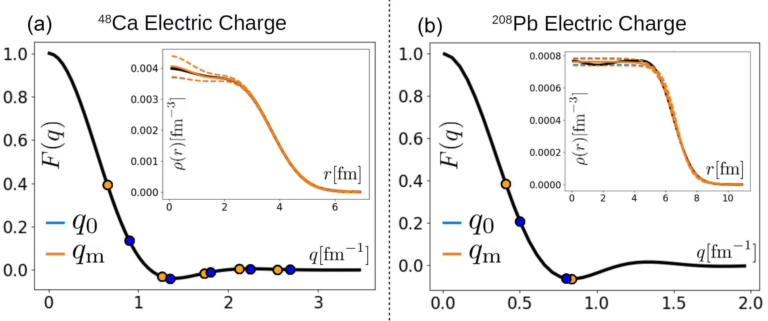

We show in Fig. 5 results obtained before and after optimizing the location of the momentum-transfer points. We display the original locations in blue and their shift to their optimal locations in orange, where the FOM is minimized subject to the following constraints: for 48Ca and for 208Pb. Beyond these limits, we assume that the experimental challenge to measure such small cross sections can not be met. This may be better appreciated by displaying the form factor in a logarithmic plot, as in Fig. 6; note that the cross section is proportional to the square of the form factor. Note that the minimization of the FOM was done by running the python numpy optimization library with the ‘TNC’ method for 10 different seeds including the original choice. In Table 2, we show results for the MSE for both nuclei in terms of their natural scales. The MSE in the interior was not substantially reduced for 48Ca and it even increased by for 208Pb, as can be seen by the slightly larger error bands in Fig. 5. On the other hand, the MSE for the radius was improved by for 48Ca and by for 208Pb. These results are driven by our selection of scales which favored an improvement in the radius rather than in the interior density. Also, the radius is an easier quantity to constrain than the interior density. Note, however, that even minimizing the FOM with only the interior term does not significantly improve the interior density.
| 48Ca | 208Pb | |||
| Int | Rad | Int | Rad | |
| MSE () | 1.27 | 1.37 | 0.27 | 0.77 |
| MSE () | 1.26 | 0.94 | 0.32 | 0.63 |
Finally, listed in Tables 3 and 4 in Appendix D are the numerical values of the times the respective error for the density at fm and the radius for two sets of locations of the momentum transfer, namely, original and optimal . These individual values illustrate how much each measurement is currently impacting the variance in the radius and in the density at . Note that in Eq.(25) each term is added in quadrature. Therefore, the final variance is not linear on each component. Indeed, the quadrature equation will enhance the effect of bigger numbers with respect to their smaller counterparts. For example, in the case 48Ca with the optimized set, the variance in is dominated by the observations at and , whereas for the radius the variance is largely driven by the form factor at . A similar analysis for 208Pb reveals that the variance in is driven by , whereas the measurement at dominates the variance in the radius. Given that the radius is obtained from the slope of the form factor at zero momentum transfer and the interior density is controlled by the large-q behavior of the form factor, the previous results are fully consistent with our expectations. Note that as the errors in the observations change, these statements might no longer hold true. Our main conclusion is that to reduce the final variance on each quantity within this hypothetical experimental design—and to first approximation—these are the critical data locations that should be targeted for error reduction.
IV.2 Weak Charge Densities
We now proceed to compare the performance of each of the seven models mentioned in Sec. II.2 in reproducing the interior density and radius of the weak charge distribution of 48Ca and 208Pb. Appendix D presents the corresponding analysis for the charge densities.
Given that there is no experimental information on the weak charge form factors of 48Ca and 208Pb, we use Eq.(20) to calculate the squared average MSE from the five different generators obtained from Ref. Chen and Piekarewicz 2015, namely, RMF012, RMF016, RMF022, RMF028 and RMF032. As in the previous section, we start with five fixed locations and then optimize these values to to minimize the average FOM. We apply the same restrictions as in the example of the charge density: for 48Ca and for 208Pb. Note that since the goal is to minimize the average mean-square error of all five generators, the resulting optimal values only depend on the choice of the model. The starting locations for the momentum transfer in the case of 48Ca are once again fixed at , whereas for 208Pb they are now chosen at . Note that these values correspond to the special choice of for , with the cutoff radius for 48Ca Lin and Horowitz 2015b and for 208Pb.


In Figures 7 and 8 we display the performance of the seven models employed in the text to describe the weak charge of 48Ca and 208Pb, respectively. Shown in each figure are the resulting bias, standard deviation (SD), and MSE for the interior density (three bars on the left of each panel) and the weak charge radius (three bars on the right of each panel). The corresponding figures for the electric charge density are shown in Figures 11 and 12 in Appendix D. We note that for a fixed model we obtained very similar results regardless of the particular RMF generator; as an example see Figures 13 and 14 in Appendix E. This suggests that the conclusions that we draw within each model are robust, at least within the (RMF) family of generators considered in this study.
We want to highlight two main points from these results. First, changing the data locations (i.e., the selection of the various momentum transfers) has a significant impact on the performance of the model. For example, in the description of the weak charge density of 208Pb the performance of the Helm model improves by nearly a factor of two. Second, we observe large variations in the model performance when the original fixed locations are adopted. Indeed, for 48Ca the performance of the Bessel-Fourier expansion outperforms that of the SF+B model by about a factor of two. Such large discrepancy is often mitigated by selecting the optimal locations for each model; see the dramatic improvement in the description of the weak charge radius of 208Pb when the optimal locations are adopted. Based on these two points, we can conclude that the optimal model will strongly depend on the data structure, regarding both locations and errors. We should expect that variance driven models (like the Bessels) will outperform bias driven models (like the SF) in cases where the data errors are small. For the number of experimental measurements and errors assumed in this example, the Helm and SF models are best suited for the simultaneous extraction of the radius and interior density of both nuclei. This could be expected for the case of 208Pb given that both the Helm and SF models are characterized by a flat interior density that provides our closest connection to the saturation density of infinite nuclear matter Horowitz et al. 2020. It might come as a surprise that these flat models outperform more flexible models like the Bessel-Fourier expansion which better describes the interior shell oscillations of 48Ca. The reason behind this finding is that we aim to minimize the MSE, which involves a combination of the bias and the variance. On average (mean value), the Bessel model will provide a more genuine representation of the interior oscillations of the weak charge density of 48Ca. However, the noise level as quantified by the variance is so high that the expected deviation is large enough to make more desirable a flat description with smaller error bands.
As an example, consider the RMF012 generator displayed as the black solid curve in Fig 4(a). This RMF generator predicts a weak charge density for 48Ca that is slightly enhanced at relative to the average interior density and then drops from the average around . We could then ask: how probable is it to conclude the opposite (i.e., ) after adopting the optimal locations for the Bessel model. To answer that question, let us define the new quantity of interest and investigate the probability that . Once the optimal values are adopted, an average value of is obtained, suggesting that , in agreement with the predictions from the RMF012 generator. But what about the variance in this result? The variance of this quantity can be calculated using the TF formalism from Eq. (25) as:
| (38) |
where we have used Eq.(22) and Eq.(24) to write the explicit form of . Following this procedure, we obtain a standard deviation of . We note that the third measurement at has the largest impact on the the variance, followed by appreciable contributions from and ; see Table 5 in Appendix D for the values of . Hence, under the assumption that the errors are Gaussian distributed random variables, we can infers that in of the experimental realizations. That is, if the experimental noise (primarily in , and ) cannot be significantly reduced, we will conclude the incorrect oscillation structure in the interior density of 48Ca in one out of six experiments.
For the interior density of 208Pb, the best overall score was achieved by the SF model with a total MSE of , where is defined in Table 1. Using again RMF012 as an example of a generator, we observe that the total variance in is mainly driven by the third observation, having a value of . Taking as a representative value of the interior density, this implies that the measurement at should be primarily targeted for error reduction in order to improve the uncertainty in the saturation density . We underscore that the interior density of 208Pb is a genuine experimental observable that provides the closest connection to the saturation density of infinite nuclear matter. For a recent analysis on how a measurement of the interior density of 208Pb could constraint see Ref. Horowitz et al. 2020.
In the case of the weak charge radii of both nuclei, we found that they can be accurately determined using the Helm model: an MSE of fm for 48Ca and of fm for 208Pb, with both values of listed in Table 1. In the case of 48Ca, and relying again on RMF012, the total variance in is uniformly distributed among the first three observations at , , and , with values of . Instead, for 208Pb we found that the total variance in is driven by the two points closest to the origin, namely, and , with values of . To improve the uncertainty in the weak charge radii, the observations at these “low-q” points should be targeted for error reduction. These results are hardly surprising given that the weak charge radius is defined in terms of the slope of the associated form factor at the origin. It is worth noting that the weak charge radius of 208Pb, when combined with the corresponding (electric) charge radius into a neutron skin, provides a stringent constraint on the slope of the symmetry energy —and ultimately on the radius of neutron stars Horowitz and Piekarewicz 2001b. In particular, a 1% determination of the weak charge radius of 208Pb translates into an uncertainty of about MeV in the slope of the symmetry energy Horowitz et al. 2014b.
IV.3 The role of priors
The incorporation of priors lies at the heart of Bayesian statistics. Priors allow us to include physical biases and intuition as well as information from previous experiments. Moreover, priors play the important role of serving as leverage to reduce the variance of a model at the expense of increasing its bias Bishop 2006; Sullivan 2015. This can be particularly beneficial for models such as the Bessel-Fourier expansion or SF+G, whose MSE is largely driven by the variance given the level of noise in the generated data.

In this section, we briefly explore the impact of an informed prior on the performance of the SF+G model as it pertains to the weak charge density of 48Ca. As we have done earlier, we use the RMF012 generator to produce synthetic data. The proposed locations of the measurements are the original five values of the momentum transfer: . Note that the implementation of priors was discussed in Sec. II.2.2 and extended to the TF formalism in Sec. III.4. The SF+G model consists of the two-parameter symmetrized Fermi function plus three Gaussians “bumps” to account for shell oscillations in the interior. The Gaussians are centered in the interior at three different locations: fm. We analyze three prior options for the amplitude of the Gaussians (), while we leave the two intrinsic parameters of the SF model unconstrained. First, we consider a null prior that we refer to as . Such “prior” effectively reproduces the original unconstrained SF+G model. Second, we consider a fairly uninformed prior, defined in such a way that the deviation from a flat density at the peak of each Gaussian is of the order of fm-3, or roughly of the average interior density. We call this prior and is given by the following parameter centers and standard deviations:
| (39) |
Finally, we consider an extremely restrictive prior () that forces the value of all three Gaussian amplitudes to zero (), effectively reproducing the original flat SF model without oscillations. For an example on the incorporation of priors see Appendix F.
The reconstructed weak charge density of 48Ca for the three choices of priors is displayed in Fig. 9(a), with (in blue) displaying the largest variance, (in green), and (in orange) displaying the smallest variance but the largest bias. The overall performance for each choice is quantified in Fig. 9(b). These results are an interesting example of the bias vs variance trade-off: the model without prior () reproduces the true (RMF012) curve almost perfectly, but displays a huge error band, whereas the model with the most restrictive prior (), or effectively with the fewer number of parameters, has the largest bias but the smallest error bands (variance). Note that and have almost the same overall MSE score. Also note that since what can be measured is the form factor as a function of the momentum transfer, the reconstructed spatial density in the interior does not have to be well constrained if there are not enough data. This is the main reason that the orange curve () that fails to reproduce the interior oscillations, also fails to reproduce the average interior density. The model with the prior provides the best overall MSE score. Indeed, its MSE score is even better than any of the average MSE scores of the models studied in Sec. IV.2, for fixed locations.
We can analyze the behavior of the MSE directly from the transfer function formalism as the prior is modified. To do so, let us focus on the interior density . Stronger priors constrain more effectively , thereby reducing the impact of the transfer functions of each data point. This effectively reduces the propagation of experimental uncertainty towards the calculated variance in . The trade-off is due to the fact that the inclusion of a strong prior will push away the central value of from what the central values of the data () suggest, resulting in an increase of the total bias in . Such a change can be written to first approximation as:
| (40) |
where the are now defined as the difference between the parameter’s value without priors and the new prior centers .
Appendix F includes tables with the numerical values of the transfer functions for and clarifies their meaning in more detail. The important fact is that, as the prior strength increases from to , the numerical value of the for each observation tends to decrease—sometimes by an order of magnitude. This leads to a dramatic decrease in the total variance in the interior density. On the other hand, as the prior strength increases, the prior transfer functions become stronger. This allows each prior center to push away the value of from what the data suggest, effectively increasing the bias.
The example highlights how a well chosen prior could be crucial to reduce uncertainties. However, if the prior strength is excessively high, there is the risk of overlooking new discoveries or making erroneous conclusions. A more in depth analysis is required to optimize the prior strength and structure for each particular problem in order to effectively reduce the MSE for a set of given truths.
V Conclusions and future directions
In this paper, we proposed a novel statistical framework–the transfer function (TF) formalism–and applied to the extraction of nuclear densities from the associated form factors obtained from electron-scattering data. From this new perspective, we explored: model selection and model building, the impact of data locations and errors, the role of priors, and the bias vs variance trade-off. Given the importance of the PREX and CREX campaigns at JLab in constraining the density dependence of the symmetry energy and in bridging ab-initio descriptions to density functional theory, we focused our analysis on 48Ca and 208Pb. In particular, the two observables of interest explored in this work were the mean square radii and interior densities of both neutron-rich nuclei. We evaluated the performance of seven models in faithfully reproducing these two observables, from noisy experimental data on the electric form factor and noisy pseudo-data generated from a variety of relativistic mean field models for the case of the weak-charge form factor. The performance of the various models was quantified in terms of the Mean Squared Error (MSE) defined as a combined score obtained from incorporating both the bias and the variance.
For both the charge and weak charge densities we showed that, for the adopted noise level assumed in the data, the best performance was obtained with the simpler SF and Helm models that are characterized by a flat interior density. More complex models such as the SF+G or a Fourier-Bessel expansion did not perform as well. Whereas both of these more complex models are able to reproduce the interior shell oscillations of both nuclei, they are hindered by a very high variance, which ultimately results in a high MSE score. In this regard, we suggest that it will be difficult for any of the models used in this paper—at least in their present form—to faithfully reproduce the shell oscillation of both nuclei, particularly in the case of 48Ca where the oscillation structure is expected to be more pronounced. Indeed, when using the Fourier-Bessel expansion as in Lin and Horowitz 2015b, we estimated that there is a chance of predicting the wrong oscillating structure in the interior of 48Ca, namely, peaks become valleys and valleys become peaks.
In the context of experimental design, we illustrated how to use the TF formalism to identify those critical observations that are driving most of the uncertainty in our estimations. The identification of those critical points could help in the design of future experiments to allocate more resources (e.g., beam time) to those critical locations to maximize the information gained from such experiments. Finally, we explored the impact of priors on the extracted weak charge density of 48Ca under the SF+G model. As the influence of the prior increased, so did the bias while the variance was reduced—as expected from the bias vs variance trade-off.
Going forward, there are several directions that are worth exploring. First, it would be interesting to integrate the TF formalism directly into model building. We believe questions such as what makes a model better than others?, could be tackled from the TF perspective. Answering which model is better at extracting data has become a central question in nuclear physics, for example in the context of the proton puzzle. Yan et al., investigated this question and provided fundamental insights to the analysis by the PRaD collaboration. This seminal work—which inspired a great portion of the development of the TF formalism—identified the models optimally suited to extract the proton radius, but did not elaborate on what made those model successful. We believe the TF formalism could be used to make significant advances in that direction. As shown in this paper, the TF formalism seems to be ideal to identify the delicate interplay between signal and noise. Understanding the TF distribution of successful models could help not only in identifying but also in creating, some sort of “optimal” model. This technique could be applied beyond density reconstruction from scattering data as implemented in this paper, to more general problems that involve the calibration of model parameters from experimental data.
Another fruitful direction of investigation is the role of priors and hyperparameters. Hyperparameters, such as and the Gaussian locations for the SF+G, or the Bessel cut off radius and number of coefficients, can drastically impact the performance of a model. In the context of the TF formalism, we could ask questions like: Given six observations, is it better in terms of an overall MSE score, to have 5 or 6 adjustable Fourier-Bessel coefficients? How does the answer scale with the number of data points? We believe it is possible to create a framework using the TF formalism that can tackle this type of questions in a robust and direct manner. This would allow to conduct a more informed search in the hyperparameter space of each model instead of just by trial and error. Our work showed that the incorporation of priors can have a dramatic effect on a model’s performance. After all, priors are essential ingredients of the Bayesian formalism as they encode prior beliefs before additional experimental evidence becomes available. A more in depth study should be carried out to identify how to optimize the hyperparameters that define the priors. To reach robust conclusions, such a research project should include more generator functions from other nuclear model families. We are confident that the TF formalism can guide this optimization procedure as well.
Finally, a third possible application of the TF formalism is related to the recent use in nuclear physics of Bayesian frameworks for combining different competing models to improve over the predictions of single models Neufcourt et al. 2020. Within the context of nuclear densities, using the MSE score should allow us to test the circumstances under which the mixing of several models outperforms the predicting power of a single model. It would be interesting to explore in the future the generalization of the TF formalism to Bayesian model mixing.
Acknowledgments
We are grateful to Edgard Bonilla for his help and critical observations during this project. We thank Prof. Antonio Linero for his guidance and key support. We thank Diogenes Figueroa for many useful conversations. We thank Prof. Douglas Higinbotham for introducing us to the bias vs variance analysis and for his encouragement at the beginning of the project. Finally, we thank Ana Posada for a careful read of the manuscript.
This material is based upon work supported by the U.S. Department of Energy Office of Science, Office of Nuclear Physics under Award Number DE-FG02-92ER40750
Appendix A Mathematical proofs on the TF formalism
A.1 Transfer Functions Structure
This subsection presents a formal proof on the structure of the transfer functions (Eq. (24)), namely that the first order change coefficients on the parameters due to a perturbation on observation are:
| (41) |
where is the inverse of the Hessian matrix of defined in (11) and is the gradient with respect to the parameters of the function being fit evaluated at observation .
Let us assume that we are at the minimum of the unperturbed . At this point, the condition of a minimum implies that the first derivative of with respect to all ( in total) should be zero:
| (42) |
where we use the notation to refer to the group of all observations, and the subscript “” to refer to the unperturbed variables. We call the first derivative of with respect to parameter . The are the following functions of both the parameters and the observations:
| (43) |
Now, if we perturb observation by a small amount the minimum of will move accordingly. If we want to preserve all equations (42), (there is one equation for every parameter), then the values of all should change a small amount as well to compensate. Quantitatively, this means (to first order):
| (44) |
We can arrange all equations into a matrix form:
where, since the were already first derivatives of , we can recognize the Hessian matrix . We also recognize . We therefore have:
where, since the perturbation can be made arbitrary small, we must conclude that the quantity in brackets is what were looking for. These are the linear coefficients connecting a small change in with the small change in every parameter , proving Eq. (41).
This was a constructive proof of the transfer function structure. Another approach would be to use Newton’s minimization method to find the location of the new minimum of once we make the perturbation . Newton’s method involves the same ingredients shown in Eq. (41), namely the gradient and Hessian of the scalar objective function (). The reason why the gradient does not involve all observation but just the th component, is because in Eq. (43) only the term multiplying survives. Everything else gets cancelled by the definition of the minimum.
Finally, a third approach results by invoking the implicit function theorem on the minimum conditions of . Those are equations and each one is a function of the observations and parameters, where . Under these conditions, there exists a map in a vicinity around from the bigger set of variables (the observations) to the smaller set (the parameters). The coefficients of this linear map (first derivatives) are precisely given by (41) (see Spivak 2018 pages 41-42).
A.2 Comparing the transfer function variance with the standard approach’s variance
This subsection presents a formal proof of the statement discussed at the end of Sec III.1. When the Hessian matrix (11) only involves the linear part of the model:
| (45) |
then the variance calculated using the standard approach (12), and the variance calculated using the transfer function formalism (25), are identical, namely:
| (46) | ||||
| (47) |
Let us recall that we have observations and parameters with . To prove this statement, we first observe that the matrix is built by the sum of tensor products between the gradients with themselves:
| (48) |
Therefore, can be written as the product of a matrix and its transpose as:
| (49) |
where is a matrix which columns are the gradients of :
| (50) |
We decompose and into their decomposition (see Theorem 2 in Goodall 1993):
| (51) | |||
where and are a , and a matrix, respectively. The matrix is an orthonormal matrix meaning: , where is the identity matrix. Under these conditions, we have that:
| (52) | ||||
Therefore, under the standard approach Eq. (46) is calculating the norm squared of the vector in . Let us now work with Eq. (47) and obtain a similar structure but in .
Given how is defined, we realize that:
| (53) |
where is the th vector in the canonical base of with all entries as except for an entry of in position .
Therefore, in Eq. (47), we can replace by and obtain:
| (54) | ||||
Appendix B Model descriptions
This section presents detailed information about the seven models we studied in this work. For each model, we provide: its analytic form (if available) as a function of its parameters in both coordinate space and momentum space ; a normalization condition (if any), that restricts the parameters; the mean squared radius as a function of the parameters when available, and the values of the model’s hyperparameters, if any, used in this work.
Fourier Bessel
Under this formalism Dreher et al. 1974, the density is written as:
| (55) |
where denotes the zeroth order spherical Bessel function of the first kind, are the free parameters, and is such that for . This last condition is enforced by the Hevisde theta function .
The form factor can be expressed analytically as:
| (56) | ||||
| (57) |
The normalization condition translates to:
| (58) |
The mean square radius is obtained as:
| (59) |
In this work, we use fm when analyzing 48Ca, and fm when analyzing 208Pb. We use a total of 5 adjustable for both nuclei which translates to six Bessels () due to the normalization condition.
Helm Density
The Helm density Helm 1956 is:
| (60) | ||||
where:
| (61) |
where and are the adjustable parameters, and is the error function:
| (62) |
The Helm form factor is built by the product of two form factors: a uniform “box” density inspired by the fact that nuclear matter in nuclei saturates, and a Gaussian falloff which takes into account the finite size of the nucleons:
| (63) |
where is the spherical Bessel function of first order .
The radius is given by:
| (64) |
Symmetrized Fermi Function
The Symmetrized Fermi function Sprung and Martorell 1997 is constructed as: , where is the traditional Fermi Function Woods and Saxon 1954. Its density and form factor are expressed as:
| (65) |
| (66) |
where the normalization constant is:
| (67) |
where the parameters and represent the surface diffuseness and half-density radius, respectively. The radius is given by:
| (68) |
Symmetrized Fermi Function of three and four parameters
Based on the two parameter symmetrized Fermi density, we can build a three-parameter and a four-parameter densities as:
| (69) | ||||
| (70) | ||||
The parameters and are introduced to add flexibility near to the densities and to reproduce oscillations. Due to the size of their expressions, the normalization constants and , the form factors and the radius equations are not included here but can be calculated analytically.
Symmetrized Fermi function plus Bessels (SF+B) and plus Gaussians (SF+G)
By construction the two parameter symmetrized Fermi function exhibits a flat behaviour in the interior, so it cannot describe shell oscillations (small bumps and valleys around the saturation density background). As a different approach to adding parameters as in Eqs. (69) and (70), we propose to use the following hybrid models.
SF+B:
where is the spherical Bessel function of the first kind and the Heaviside theta function. We set fm for 48Ca and fm for 208Pb. in this context specifies the region where we believe the interior oscillations are important. We use a total of three adjustable coefficients which in this case correspond to three Bessels () since the normalization is enforced automatically. We have therefore a total of five parameters including and from the SF model.
SF+G:
| (71) | ||||
where is defined as:
| (72) | ||||
The amplitudes of the Gaussians act as adjustable parameters. In our case they are not restricted to be positive in contrast with Sick 1974. We use a total of three Gaussians (), giving us five adjustable parameters including and from the SF model. The hyperparameter , which represents the common width of the Gaussians, is set to fm for both nuclei (see Sec III.5 for a discussion of this value). The center of each Gaussian is denoted by and we chose the following values:
| (73) | ||||
The main idea behind these expansions is that the principal behaviour of the nuclear density is modeled by the symmetrized Fermi density, while the fine details are modeled by either a sum of Bessels or Gaussians. Both and the are chosen in such a way that they cover the region where we expect the oscillations around a flat density to be important.
The Bessel approach has the disadvantage that the total density will present a discontinuity at . This “kink”, while nonphysical, might not preclude the entire model from describing nuclear densities.
The form factors for both densities can be expressed in analytic form:
| (74) | ||||
| (75) |
where is defined in Eq. (57), and is defined as:
| (76) |
The SF+B radius is given by:
| (77) |
The SF+G radius is given by:
Appendix C Details about the SF+G reconstruction bias analysis
This section provides a more detailed view at the reconstruction bias for the SF+G model discussed in Sec III.5. Let us recall that we are analyzing how much the placement of the fourth measurement impacts the change in through the transfer function formalism:
| (78) |
Fig. 10 ((a.1) and (b.1)) shows this calculated in black (as an absolute percentage) as moves along the possible momentum transfer range fm-1 while the other remain in position. The SF+G model with the hyperparameter fm is displayed in (a.1) while fm is used in (b.1). The x-axis of both plots shows the two original data sets of fm-1 (blue), and fm-1 (orange), which only differ in their value.

In Fig. 10 (a.1) it can be observed that for most locations the calculated exceeds the threshold (the blue dashed line). On the other hand, for (b.1) the black curve is overall lower, showing a wider region where . This overall reduction is the reason why we chose fm to perform the analysis in Sec IV.
The “spikes” where grows abruptly appear when we aim to move to the other locations, effectively measuring twice in the same spot. Since we have five parameters and five observations, this results in a non-invertible Hessian for , which blows up the transfer function . It is interesting to note that, even though there is not an observation located at fm-1, a “spike” can still be observed. This is because by definition all model form factors must respect . Therefore a measure at fm-1 provides no new information, resulting in a non-invertible Hessian as well.
Fig. 10 ((a.2) and (b.2)) shows the true form factor (RMF012) in black and the observation locations as the blue and orange points, being (a.2) for fm, and (b.2) for fm. The red squares represent “forbidden zones”, regions in the space where if we place the fourth location we obtain a bias in bigger than . For (a.2) these zones occupy around of the total range, while for (b.2) they occupy around .
By the construction in Sec III.5, locating at the blue point fm-1 will result in almost zero bias since the optimal form factor and the true form factor have the same value (). As moves away from this location, we expect the bias to increase. A “bad” model will present a bias that grows too quickly, while a “good” model will be more tolerable. As can be observed in Fig. 4, for the same fm-1, the SF+G with fm (orange dashed curve) fails to be within the band, while the SF+G with fm (red dashed line) stays within. In Fig. 10 (a.2) the orange point is covered by the red rectangle. This is not the case for (b.2).
It should be noted that changing the hyperparameter from fm to fm can impact the locations where since now the optimal function will be different. Nevertheless, in the case we studied here the change in these locations was negligible, a fact that simplified our discussion.
Appendix D Details about the 48Ca and 208Pb charge examples and model comparison
This Appendix presents tables and details relevant to the 48Ca and 208Pb charge density example developed in Sec IV.1. It includes the results of applying the same analysis on model comparison developed in Sec IV.2 to the electric charge densities of both nuclei instead of their weak densities counterparts.
| [fm-1] | [] | 0.90 | 1.35 | 1.80 | 2.24 | 2.69 |
| [] | 0.65 | 1.26 | 1.73 | 2.12 | 2.55 | |
| [] | 0.84 | 1.02 | 1.44 | 1.07 | 0.65 | |
| [] | 0.65 | 1.18 | 1.40 | 0.90 | 0.72 | |
| [] | 0.88 | 0.80 | 0.58 | 0.32 | 0.12 | |
| [] | 0.82 | 0.34 | 0.26 | 0.15 | 0.03 |
| [fm-1] | [] | 0.50 | 0.80 |
|---|---|---|---|
| [] | 0.41 | 0.84 | |
| [] | 0.14 | 0.18 | |
| [] | 0.17 | 0.25 | |
| [] | 0.59 | 0.48 | |
| [] | 0.54 | 0.31 |
Tables 3 and 4 show for the 48Ca and 208Pb examples, respectively, the original locations as well as the locations that minimize the FOM defined in Eq. (37). Tables 3 and 4 also show the numerical values of the times the respective error for the density at fm and the radius for both data sets and . Let us recall that it is the total interior density (the 30 grid points in Eq. (36)), what goes in the FOM Eq. (37). We are using as a representative of the total interior density. All of the transfer function values have been divided by the natural scales defined in Table 1.
By adding in quadrature each element in the rows of Tables 3 and 4 (the transfer functions values times the respective errors), the total variance in or can be calculated from Eq. (25), in units of the natural scale. In this sense, each number in the table represents the contribution of that measurement to the total variance in that quantity. This allows us to identify, for example, that the variance in in the case of for 48Ca is completely driven by the first observation fm-1, while the contribution of the last point fm-1 is negligible. From an experimental design point of view, this means that if our main goal is to reduce the uncertainty in the radius, we must allocate the resources accordingly and reduce the error bar on rather than reducing the error bars in the other locations.
Figures 11 and 12 show, for 48Ca and 208Pb, respectively, the results for comparing the seven models defined in Sec II.2 to recover the interior charge density and charge radius. The numerical values shown in these Figures are written in Tables 7 and 8. Tables 5 and 6 show the associated optimal locations for every model for 48Ca and 208Pb, respectively.
| [fm-1] | |||||
|---|---|---|---|---|---|
| Bessels | 0.65 | 1.26 | 1.73 | 2.12 | 2.55 |
| Helm | 0.68 | 0.71 | 1.39 | 2.09 | 2.10 |
| SF | 0.44 | 0.62 | 1.24 | 2.09 | 2.79 |
| SF3 | 0.56 | 0.90 | 1.20 | 1.84 | 2.50 |
| SF4 | 0.50 | 1.10 | 1.92 | 2.12 | 2.59 |
| SF+B | 0.67 | 1.31 | 1.80 | 2.43 | 3.20 |
| SF+G | 0.63 | 1.25 | 1.78 | 2.17 | 2.80 |
| [fm-1] | |||||
|---|---|---|---|---|---|
| Bessels | 0.37 | 0.86 | 1.20 | 1.60 | 1.80 |
| Helm | 0.41 | 0.43 | 0.83 | 0.88 | 1.31 |
| SF | 0.42 | 0.43 | 0.83 | 0.87 | 0.88 |
| SF3 | 0.23 | 0.41 | 0.88 | 1.07 | 1.16 |
| SF4 | 0.25 | 0.36 | 0.70 | 1.22 | 1.51 |
| SF+B | 0.38 | 0.87 | 1.27 | 1.75 | 1.97 |
| SF+G | 0.36 | 0.90 | 1.29 | 1.68 | 1.91 |
We judge each model by their individual bias, standard deviation, and MSE both in the original locations as well as the optimized locations where the FOM is minimized. As we did in Sec IV.2, the starting locations are fm-1 for 48Ca and fm-1 for 208Pb.
| Interior | Radius | Interior | Radius | |||||||||
| Bias | SD | MSE | Bias | SD | MSE | Bias | SD | MSE | Bias | SD | MSE | |
| Bessels | 0.15 | 1.26 | 1.27 | 0.05 | 1.37 | 1.37 | 0.19 | 1.24 | 1.25 | 0.00 | 0.96 | 0.96 |
| Helm | 0.50 | 0.54 | 0.73 | 0.72 | 0.73 | 1.03 | 0.51 | 0.55 | 0.75 | 0.12 | 0.49 | 0.50 |
| SF | 0.59 | 0.51 | 0.78 | 1.28 | 0.85 | 1.54 | 0.48 | 0.49 | 0.68 | 0.37 | 0.67 | 0.77 |
| SF3 | 0.62 | 0.83 | 1.04 | 1.33 | 1.04 | 1.68 | 0.34 | 0.66 | 0.74 | 0.29 | 0.84 | 0.88 |
| SF4 | 0.75 | 1.00 | 1.25 | 0.31 | 4.38 | 4.40 | 0.73 | 1.01 | 1.25 | 0.08 | 1.38 | 1.38 |
| SF+B | 1.47 | 3.00 | 3.35 | 0.42 | 1.46 | 1.52 | 0.12 | 1.46 | 1.47 | 0.30 | 0.86 | 0.92 |
| SF+G | 0.37 | 1.48 | 1.52 | 0.32 | 1.71 | 1.74 | 0.26 | 1.39 | 1.41 | 0.13 | 0.97 | 0.98 |
| Interior | Radius | Interior | Radius | |||||||||
| Bias | SD | MSE | Bias | SD | MSE | Bias | SD | MSE | Bias | SD | MSE | |
| Bessels | 0.44 | 1.95 | 2.00 | 0.02 | 1.88 | 1.88 | 0.48 | 1.82 | 1.89 | 0.08 | 0.74 | 0.74 |
| Helm | 0.17 | 0.22 | 0.28 | 0.30 | 0.91 | 0.96 | 0.14 | 0.19 | 0.24 | 0.04 | 0.41 | 0.41 |
| SF | 0.17 | 0.22 | 0.28 | 0.20 | 1.06 | 1.08 | 0.16 | 0.19 | 0.24 | 0.09 | 0.42 | 0.43 |
| SF3 | 0.15 | 0.58 | 0.60 | 0.55 | 1.40 | 1.50 | 0.10 | 0.45 | 0.46 | 0.19 | 0.59 | 0.62 |
| SF4 | 0.19 | 0.73 | 0.76 | 0.17 | 3.59 | 3.59 | 0.18 | 0.76 | 0.78 | 0.09 | 0.72 | 0.72 |
| SF+B | 0.17 | 2.86 | 2.86 | 0.36 | 1.60 | 1.64 | 0.17 | 2.43 | 2.44 | 0.21 | 0.69 | 0.72 |
| SF+G | 0.13 | 2.64 | 2.64 | 0.35 | 1.72 | 1.75 | 0.17 | 2.50 | 2.51 | 0.19 | 0.74 | 0.76 |


We observe similar trends as the one displayed by Figures 7 and 8 when comparing models for the weak charge densities. Changing the data locations can result in an important reduction of the MSE, for example by a factor of two by the SF in the 48Ca radius. There are also significant variations in performance among the models, for example a factor of three between the SF+B and SF+G when compared to the Helm model when extracting the interior density of 208Pb for . Once again, for the data range and errors we have assumed, the Helm and SF model seem to outperform all of the other options in both nuclei.
Finally, it is interesting to analyze the distribution of optimal locations for the seven models in Tables 5 and 6. Let us recall that we limited the maximum value of any to be less than fm-1 for 48Ca and less than fm-1 for 208Pb. Although there is no clear pattern, both the SF and Helm models seem to have overall smaller values of , while the models involving Bessels seem to be more in the high end. Depending on the experiment details and constraints, some regions of the space would be easier to access than others. In that case, a more detailed analysis could be done to optimize a modified version of the FOM in which we take into account the experimental budget. It is very likely that the FOM would not be extremely sensitive to the exact locations of . Therefore, an adjustment of each could result in a notorious reduction of the experimental budget while the FOM deteriorates just a small amount.
Appendix E Details about the 48Ca and 208Pb weak charge analysis
This appendix presents tables and details relevant to the 48Ca and 208Pb weak charge density model comparison developed in Sec IV.2. The numerical values associated with Figures 7 and 8 are shown in Tables 11 and 12, respectively. Tables 9 and 10 show the associated optimal locations for every model for 48Ca and 208Pb, respectively.
| [fm-1] | |||||
|---|---|---|---|---|---|
| Bessels | 0.71 | 1.32 | 1.81 | 2.28 | 2.65 |
| Helm | 0.51 | 0.63 | 0.77 | 1.44 | 2.93 |
| SF | 0.74 | 0.92 | 1.36 | 1.67 | 2.50 |
| SF3 | 0.54 | 1.32 | 1.69 | 1.87 | 2.42 |
| SF4 | 0.44 | 1.41 | 2.10 | 2.82 | 2.88 |
| SF+B | 0.61 | 1.26 | 1.78 | 2.32 | 3.03 |
| SF+G | 0.57 | 1.18 | 1.69 | 2.06 | 2.68 |
| [fm-1] | |||||
|---|---|---|---|---|---|
| Bessels | 0.37 | 0.84 | 1.21 | 1.61 | 1.80 |
| Helm | 0.37 | 0.40 | 0.84 | 1.23 | 1.24 |
| SF | 0.37 | 0.40 | 0.77 | 0.84 | 1.36 |
| SF3 | 0.38 | 0.43 | 0.87 | 1.03 | 1.17 |
| SF4 | 0.32 | 0.52 | 0.68 | 0.81 | 1.09 |
| SF+B | 0.37 | 0.84 | 1.25 | 1.70 | 1.94 |
| SF+G | 0.32 | 0.82 | 1.23 | 1.65 | 1.85 |
| Interior | Radius | Interior | Radius | |||||||||
| Bias | SD | MSE | Bias | SD | MSE | Bias | SD | MSE | Bias | SD | MSE | |
| Bessels | 0.09 | 1.26 | 1.26 | 0.06 | 1.31 | 1.31 | 0.08 | 1.30 | 1.31 | 0.30 | 0.87 | 0.92 |
| Helm | 1.22 | 0.50 | 1.32 | 1.08 | 0.87 | 1.39 | 0.70 | 0.56 | 0.90 | 0.03 | 0.45 | 0.45 |
| SF | 1.09 | 0.47 | 1.19 | 0.87 | 1.04 | 1.37 | 0.62 | 0.41 | 0.74 | 0.24 | 0.76 | 0.81 |
| SF3 | 1.20 | 0.86 | 1.47 | 2.14 | 1.18 | 2.44 | 0.60 | 0.93 | 1.11 | 1.04 | 0.94 | 1.40 |
| SF4 | 0.94 | 1.39 | 1.68 | 2.71 | 1.70 | 3.22 | 0.63 | 1.62 | 1.74 | 1.23 | 1.10 | 1.65 |
| SF+B | 0.70 | 2.37 | 2.47 | 1.04 | 1.83 | 2.10 | 0.17 | 1.47 | 1.48 | 0.90 | 0.95 | 1.31 |
| SF+G | 0.19 | 1.44 | 1.45 | 1.02 | 2.25 | 2.47 | 0.22 | 1.35 | 1.36 | 0.82 | 1.11 | 1.38 |
| Interior | Radius | Interior | Radius | |||||||||
| Bias | SD | MSE | Bias | SD | MSE | Bias | SD | MSE | Bias | SD | MSE | |
| Bessels | 0.20 | 1.95 | 1.96 | 0.40 | 1.82 | 1.86 | 0.36 | 1.83 | 1.87 | 0.05 | 0.70 | 0.71 |
| Helm | 0.10 | 0.23 | 0.25 | 0.59 | 1.11 | 1.26 | 0.11 | 0.21 | 0.24 | 0.01 | 0.45 | 0.45 |
| SF | 0.09 | 0.22 | 0.24 | 0.28 | 1.40 | 1.43 | 0.09 | 0.19 | 0.21 | 0.25 | 0.47 | 0.53 |
| SF3 | 0.15 | 0.59 | 0.61 | 0.51 | 1.99 | 2.06 | 0.10 | 0.40 | 0.41 | 0.29 | 0.62 | 0.69 |
| SF4 | 0.14 | 0.77 | 0.78 | 0.61 | 4.08 | 4.13 | 0.14 | 0.60 | 0.62 | 0.21 | 0.83 | 0.86 |
| SF+B | 0.13 | 2.70 | 2.70 | 0.46 | 2.19 | 2.24 | 0.15 | 2.40 | 2.41 | 0.31 | 0.78 | 0.84 |
| SF+G | 0.19 | 2.56 | 2.57 | 0.47 | 2.50 | 2.54 | 0.26 | 2.48 | 2.49 | 0.27 | 0.82 | 0.87 |


As done in Appendix D, we can analyze the distribution of these optimal locations . We observe a similar structure from their charge counterparts: no clear pattern but both SF and Helm models seem to have overall smaller values of , while the models involving Bessels seems to be more in the high end.
Since parity violating experiments are extremely expensive and challenging, the experimental constraints and budget should definitely be considered in a more detailed analysis to optimize a modified version of the FOM. We again anticipate that the FOM will not be extremely sensitive to the exact locations of , and that an adjustment of each could result in a huge impact on the budget while the FOM deteriorates just a small amount. This analysis could also change our conclusions regarding the optimal models. For example, for the weak results of 208Pb, the Helm model seems to have a better FOM combination than the SF, but it could be that the from the SF model are more experimentally accessible than those from the Helm model.
Finally, Figures 13 and 14 show, as an example, the detailed results of the Bessels model for 48Ca and the SF model for 208Pb, respectively, across the five different generators used in Sec IV.2. The last columns on each figure show the squared average (see Eq. 20) of each quantity (bias, SD, and MSE), which corresponds to the single values displayed in Figures 7 and 8 in the main text. As can be seen, the variations among different generators are very small. We interpret this as a sign that our conclusions are robust at least within the family of generators we considered in this study.
Appendix F Details about the role of priors
This section presents tables with the numerical values of the transfer functions of both the data and the priors related to what was discussed in Sec IV.3. Let us recall that we are using the SF+G model with three scenarios for the prior. In terms of their strength these are: 1) : no prior (unconstrained SF+G); 2) : the specified prior in Eq. (39); and 3) : a very restrictive prior which makes the SF+G practically behave as the SF model without Gaussians.
| 1.06 | 0.46 | 2.38 | 0.35 | 1.10 | |
| 0.68 | 0.78 | 0.64 | 0.47 | 0.20 | |
| 0.40 | 0.16 | 0.16 | 0.09 | 0.20 |
Table 13 shows the numerical value of for the five different locations and for the three different priors. Let us recall that the FOM in Eq. (37), is calculated using the entire interior density, but in this section we are focusing in as a representative. For each scenario, the total contribution of the data in the variance on the density at , namely , is obtained by adding the numbers in Table 13 in quadrature22 2 The position fm is only one of the 30 grid points in Eq. (36). The total interior MSE will receive contributions not only from .. In this sense, each number in the table reflects how much that particular data point uncertainty contributes to the total band that surrounds in Fig. 9, in units of the natural scale from Table 1.
It can be observed that as the prior strength increases, the influence of each data point uncertainty tends to decrease, in some cases even by an order of magnitude. This reflects the fact that models constrained by priors, which are in some sense less complex, will present a smaller variance. From the transfer function point of view, this is driven by a more constrained (see Eq. (18)).
To get a complete picture in terms of standard deviation, we must also look at the variance introduced by the addition of the prior itself. In Eq. (16a), we can see that each Gaussian prior has an associated center , and “error” which are analogous to the true observations and true error of the data in Eq. (10). Although is more constrained, we now have to take into account the transfer functions () associated with the fact that in principle could fluctuate around its center by as much as (to 1 sigma).
The scenario without prior does not present these transfer functions. The scenario with the extremely constrained prior does not present the transfer functions either since it is as if the parameters associated with the Gaussians were not there in the first place (also, we have observed that numerically when ). Table 14 shows in the case of the intermediate prior the numerical value of these times their respective uncertainty in terms of the natural scale . The total variance in for the model with this prior is calculated by adding in quadrature these values plus the ones associated with the data in Table 13.
| 0.89 | 0.24 | 0.58 |
We can also describe the induced bias by the inclusion of a prior, i.e., how the estimated central value of is impacted by the new prior. This description is done in terms of the prior transfer functions by analyzing how the parameters (those obtained in the absence of a prior) move to either or (the fitted parameters when using prior or ). The reasoning is similar to the discussion about the and how they moved the fitted parameters away from the optimal value .
Suppose that we are currently at and we add a prior term to (converting it to defined in Eq. (17)) in such a way that the centers fall exactly at the value of their respective parameters , then the central value of the fitted parameters will not change by the addition of that prior. As a concrete example, let us assume that when the data are fitted, the value of the first unconstrained parameters (A1) is . Then, if we add to the total a prior term of the form:
| (79) |
and fit the parameters again, we will obtain the same values for all the parameters (the Hessian would be more restricted, but the center location will be intact). Now, let us imagine that we “perturb” the value of the center (in the example 0.005), and move it to the original location of the prior we want to enforce (either or ). This change, which we call , will now produce a change in the value of the parameters and therefore, in :
| (80) |
where , the difference between the parameter’s value without priors and the new prior centers. Table 15 shows in units of , the predicted change driven by the inclusions of the prior in the three amplitudes of the Gaussians for and .
To obtain the total predicted change in (in units of ), we must add all numbers in each row. Due to the fact that they alternate signs for this example, the total change in the case with the stronger prior ends up being smaller than the intermediate strength. However, we can appreciate that as the prior strength increases, the influence of its transfer functions increases by a factor between and . We interpret this as an increase in the bias of the model as compared to its priorless counterpart.
| 5.1 | -0.17 | -2.7 | |
|---|---|---|---|
| 10 | 0.64 | -11 |
Finally, note that Eq(80) is just a linear approximation. Nonlinear models will deviate from the predictions of this linear approximation if the parameters change considerably. In this particular case, the predictions on are within of the true change obtained when re-fitting the parameters with the new priors. Even though the numerical accuracy is not perfect, these types of analysis can help in better estimating the bias vs variance trade-off when including priors.
References
- von Weizsäcker (1935) C. F. von Weizsäcker, Z. Physik 96, 431 (1935).
- Bethe and Bacher (1936) H. A. Bethe and R. F. Bacher, Rev. Mod. Phys. 8, 82 (1936).
- Fricke et al. (1995) G. Fricke, C. Bernhardt, K. Heilig, L. A. Schaller, L. Schellenberg, E. B. Shera, and C. W. de Jager, Atom. Data and Nucl. Data Tables 60, 177 (1995).
- Angeli and Marinova (2013) I. Angeli and K. Marinova, At. Data Nucl. Data Tables 99, 69 (2013).
- Hofstadter (1956) R. Hofstadter, Rev. Mod. Phys. 28, 214 (1956).
- Walecka (2001) J. D. Walecka, “Electron scattering for nuclear and nucleon structure,” (Cambridge University Press, New York, 2001).
- Androic et al. (2013) D. Androic et al., Phys.Rev.Lett. 111, 141803 (2013).
- Androic et al. (2018) D. Androic et al., Nature 557, 207 (2018).
- Thiel et al. (2019) M. Thiel, C. Sfienti, J. Piekarewicz, C. J. Horowitz, and M. Vanderhaeghen, J. Phys. G46, 093003 (2019).
- Horowitz et al. (2020) C. Horowitz, J. Piekarewicz, and B. Reed, (2020), arXiv:2007.07117 [nucl-th] .
- Scholberg (2006) K. Scholberg, Phys. Rev. D73, 033005 (2006).
- Yang et al. (2019) J. Yang, J. A. Hernandez, and J. Piekarewicz, Phys. Rev. C 100, 054301 (2019).
- Freedman (1974) D. Z. Freedman, Phys. Rev. D9, 1389 (1974).
- Akimov et al. (2017) D. Akimov et al., Science 357, 1123 (2017).
- Akimov et al. (2019) D. Akimov et al., Phys. Rev. D 100, 115020 (2019).
- Donnelly et al. (1989) T. Donnelly, J. Dubach, and I. Sick, Nucl. Phys. A503, 589 (1989).
- Abrahamyan et al. (2012) S. Abrahamyan, Z. Ahmed, H. Albataineh, K. Aniol, D. S. Armstrong, et al., Phys. Rev. Lett. 108, 112502 (2012).
- Horowitz et al. (2012) C. J. Horowitz, Z. Ahmed, C. M. Jen, A. Rakhman, P. A. Souder, et al., Phys. Rev. C85, 032501 (2012).
- Adhikari et al. (2021) D. Adhikari et al., (2021), arXiv:2102.10767 [nucl-ex] .
- (20) “CREX: Parity-violating measurement of the weak charge distribution of 48Ca,” http://hallaweb.jlab.org/parity/prex/c-rex/c-rex.pdf.
- Horowitz et al. (2014a) C. J. Horowitz, K. S. Kumar, and R. Michaels, Eur. Phys. J. A50, 48 (2014a).
- Becker et al. (2018) D. Becker et al., (2018), 10.1140/epja/i2018-12611-6, arXiv:1802.04759 [nucl-ex] .
- Brown (2000) B. A. Brown, Phys. Rev. Lett. 85, 5296 (2000).
- Furnstahl (2002) R. J. Furnstahl, Nucl. Phys. A706, 85 (2002).
- Centelles et al. (2009) M. Centelles, X. Roca-Maza, X. Viñas, and M. Warda, Phys. Rev. Lett. 102, 122502 (2009).
- Roca-Maza et al. (2011) X. Roca-Maza, M. Centelles, X. Viñas, and M. Warda, Phys. Rev. Lett. 106, 252501 (2011).
- Horowitz and Piekarewicz (2001a) C. J. Horowitz and J. Piekarewicz, Phys. Rev. Lett. 86, 5647 (2001a).
- Horowitz and Piekarewicz (2001b) C. J. Horowitz and J. Piekarewicz, Phys. Rev. C64, 062802 (2001b).
- Carriere et al. (2003) J. Carriere, C. J. Horowitz, and J. Piekarewicz, Astrophys. J. 593, 463 (2003).
- Steiner et al. (2005) A. W. Steiner, M. Prakash, J. M. Lattimer, and P. J. Ellis, Phys. Rept. 411, 325 (2005).
- Erler et al. (2013) J. Erler, C. J. Horowitz, W. Nazarewicz, M. Rafalski, and P.-G. Reinhard, Phys. Rev. C87, 044320 (2013).
- Chen and Piekarewicz (2014) W.-C. Chen and J. Piekarewicz, Phys. Rev. C90, 044305 (2014).
- Chen and Piekarewicz (2015) W.-C. Chen and J. Piekarewicz, Phys. Lett. B748, 284 (2015).
- Lin and Horowitz (2015a) Z. Lin and C. J. Horowitz, Phys. Rev. C92, 014313 (2015a).
- Piekarewicz et al. (2016a) J. Piekarewicz, A. R. Linero, P. Giuliani, and E. Chicken, Phys. Rev. C94, 034316 (2016a).
- Åström and Murray (2010) K. J. Åström and R. M. Murray, Feedback systems: an introduction for scientists and engineers (Princeton university press, 2010).
- Higinbotham et al. (2018a) D. W. Higinbotham, R. E. McClellan, S. Sirca, and X. Yan, arXiv preprint arXiv:1812.05706 (2018a).
- Gueye (2020) P. Gueye, European Physical Journal. A 56 (2020).
- Hastie et al. (2009) T. Hastie, R. Tibshirani, and J. Friedman, The elements of statistical learning: data mining, inference, and prediction (Springer Science & Business Media, 2009).
- Yan et al. (2018a) X. Yan, D. W. Higinbotham, D. Dutta, H. Gao, A. Gasparian, M. A. Khandaker, N. Liyanage, E. Pasyuk, C. Peng, and W. Xiong, Phys. Rev. C 98, 025204 (2018a).
- Higinbotham et al. (2018b) D. W. Higinbotham, P. Giuliani, R. E. McClellan, S. Sirca, and X. Yan, (2018b), arXiv:1812.05706 [physics.data-an] .
- Sullivan (2015) T. J. Sullivan, Introduction to uncertainty quantification, Vol. 63 (Springer, 2015).
- Huber (2004) P. J. Huber, Robust statistics, Vol. 523 (John Wiley & Sons, 2004).
- Cacuci (2003) D. G. Cacuci, Sensitivity and uncertainty analysis, volume I: Theory, Vol. 1 (CRC press, 2003).
- De Vries et al. (1987a) H. De Vries, C. De Jager, and C. De Vries, Atomic data and nuclear data tables 36, 495 (1987a).
- Dreher et al. (1974) B. Dreher, J. Friedrich, K. Merle, H. Rothhaas, and G. Lührs, Nuclear Physics A 235, 219 (1974).
- Helm (1956) R. H. Helm, Physical Review 104, 1466 (1956).
- Sprung and Martorell (1997) D. Sprung and J. Martorell, Journal of Physics A: Mathematical and General 30, 6525 (1997).
- Sick (1974) I. Sick, Nuclear Physics A 218, 509 (1974).
- Bevington and Robinson (2003) P. R. Bevington and D. K. Robinson, Data reduction and error analysis for the physical sciences; 3rd ed. (McGraw-Hill, New York, NY, 2003).
- Gregory (2005) P. C. Gregory, “Bayesian logical data analysis for the physical sciences,” (Cambridge University Press, Cambridge, UK, 2005).
- Stone (2013) J. V. Stone, “Bayes’ rule: A tutorial introduction to bayesian analysis,” (Sebtel Press, Sheffield, UK, 2013).
- Yan et al. (2018b) X. Yan, D. W. Higinbotham, D. Dutta, H. Gao, A. Gasparian, M. A. Khandaker, N. Liyanage, E. Pasyuk, C. Peng, and W. Xiong, Physical Review C 98, 025204 (2018b).
- Piekarewicz et al. (2016b) J. Piekarewicz, A. Linero, P. Giuliani, and E. Chicken, Physical Review C 94, 034316 (2016b).
- Lin and Horowitz (2015b) Z. Lin and C. Horowitz, Physical Review C 92, 014313 (2015b).
- Van der Vaart (2000) A. W. Van der Vaart, Asymptotic statistics (Cambridge university press, 2000).
- De Vries et al. (1987b) H. De Vries, C. W. De Jager, and C. De Vries, Atom. Data Nucl. Data Tabl. 36, 495 (1987b).
- Horowitz et al. (2014b) C. J. Horowitz, E. F. Brown, Y. Kim, W. G. Lynch, R. Michaels, et al., J. Phys. G41, 093001 (2014b).
- Bishop (2006) C. M. Bishop, Pattern recognition and machine learning (Springer, 2006).
- Neufcourt et al. (2020) L. Neufcourt, Y. Cao, S. A. Giuliani, W. Nazarewicz, E. Olsen, O. B. Tarasov, et al., Physical Review C 101, 044307 (2020).
- Spivak (2018) M. Spivak, Calculus on manifolds: a modern approach to classical theorems of advanced calculus (CRC press, 2018).
- Goodall (1993) C. R. Goodall, (1993).
- Woods and Saxon (1954) R. D. Woods and D. S. Saxon, Physical Review 95, 577 (1954).