Study of Einstein-bumblebee gravity with Kerr-Sen-like solution in the presence of a dispersive medium

The physics of black holes has got renewed interest after the announcement of the detection of gravitational waves (GWs)GWAVE by the LIGO and VIRGO observatories and the captured image of the black hole shadow of a super-massive $\mathrm{M}87^{*}$ black hole by the EHT based on the very long baseline interferometry (VIBI) EHT1; EHT2; EHT3; EHT4; EHT5; EHT6. The shadow of black-hole is well studied from the theory of General relativity. A black hole shadow is a two-dimensional dark zone in the celestial sphere caused by the strong gravity of the black hole. In the article SYNGE0, Synge studied the shadow of the Schwarzschild black hole, which was then termed as the escape cone of light. The radius of the shadow of the black hole was calculated in terms of the mass of the black hole and the radial coordinate where the observer is located. In general, the shadow of a non-rotating black hole is a standard circle, whereas it is known that the shadow of a rotating black hole is not a circular disk. The different features of the black hole have been widely investigated for various gravity backgrounds, adopting an almost similar approach based on classical dynamics KHS; AMARS; ATAMS; WEIS; ABDUS; FATS; UPAPS; GRENS; ZLIS; STUC; MGAS; GHOSS; SGGS; GSBS; KUMARS; MANNS; MKHOD1; MKHOD2.

In General Relativity, light is attributed to the null geodesic of the spacetime metric and the in-medium effect, which is negligible for most of the frequency ranges, is significant for the radio frequency range. In this context, it is worth mentioning the impact of Solar corona on the time of travel and on the deflection angle of radio signals that come close to the Sun. Since the 1960s, this influence has been routinely observed. In this case, one may assume that the medium is a non-magnetized pressureless plasma and for the gravitational field, the linearized theory is sufficient. The relevant theoretical development has been made by Muhleman et al. in the articles DOM1; DOM2. With the available information, the shadow of black holes in presence of plasma has become an interesting field of research for physicists since there is a good reason for considering that black holes and other compact objects are surrounded by plasma. So, naturally, interest grows to investigate whether the presence of plasma leads to any observational effect on the radio signals and several investigations have been carried out in that direction PS1; PS2; PS3; PS4; PS5; PS6; PS7; PS8; PS9; FA; LPRO; BABAR. The physics of black holes is crucially linked with the Planck energy scale where gravity is sufficiently strong and a classical field theory of curved spacetime is not adequate to capture the finer details of the Planck scale. It needs quantization of gravity, which is not well-developed. However, it is reasonable to accept that the nature of the spacetime is discrete in that scale. Lorentz symmetry being a continuous symmetry, would not be tenable in discrete spacetime. Moreover, according to string theory, Lorentz invariance should not be an exact principle at all energy scales STRING1; STRING2; STRING3; STRING4. If Lorentz violation (LV) is considered to be a probe for the foundation of theoretical physics, then a suitable model is needed, which contains LV adopted from the standard physical principle. The known two well-developed and successful theories that describe our Universe are the theory of General Relativity and the Standard Model of particle physics. These theories are built up obeying Lorentz invariance and these two theories are applicable in two different energy scales. The standard model describes the three fundamental interactions at the quantum level, whereas general relativity describes the gravitational interaction at the classical level. A single complete theory requires the unification of these two. However, there is a strong obstacle in the way of unification since gravity can not be quantized in a straightforward manner. Therefore, a successful unified theory has not yet been developed even with huge efforts from different fronts. To unify them at very high energy scales, one builds an effective field theory termed as Standard Model Extension (SME), that couples the Standard Model to the theory of General Relativity, which involves extra items containing information about the LV happening at the Plank scale ESM1; ESM2; ESM3. The simplest case is described by a single vector bumblebee field with a nonzero vacuum expectation value and the spontaneous LV triggered by a smooth quadratic potential. Bumblebee gravitational model was first studied by Kostelecky and Samuel in STRING1; STRING2; STRING3 as a specific pattern for unprompted Lorentz violation. Therefore, the Lorentz violation aspect may be considered as a good probe on the foundation of physics.

In this context, the study of the LV effect on the shadow of a black hole in the presence of dispersive media like plasma would be of interest. There are several recent investigations to study the deformation of black hole shadow due to the LV effect CASANA0; CASANA; OUR. In these studies, the in-medium (plasma) effect has not been considered so far. Therefore, the study of the deformation of the shadow of the black hole connected with Kerr-Sen-like spacetime, the emission of energy from this black hole due to radiation, and the weak lensing in the presence of plasma would be interesting extensions. The black hole associated with Kerr-Sen-like spacetime OUR contains an LV parameter as both the Swarczschild-like and Kerr-like spacetime contain CASANA0; CASANA. This Kerr-Sen-like spacetime will enable us to study the LV effect in presence of plasma.

It is known that observation of the EHT collaboration has unveiled the first shadow image of a supermassive black hole $\mathrm{M}87^{*}$ with an asymmetric bright emission ring with a diameter of $42\pm 3\mu$$as$ exhibiting a deviation from circularity $\Delta C\leq 0.10$. It is consistent with the shadow of the Kerr black hole, but the quantitative features are not always sufficient to distinguish between black holes predicted from different theories of gravity. Thus, there is enough room for investigation concerning the viability of black holes predicted from modified theories of gravity with the help of the observed data of $\mathrm{M}87^{*}$ black hole shadow by the EHT collaboration placing constraints on the black hole parameters, and consequently, it becomes an important tool to test the phenomena of strong gravitational fields. Extensive development in this direction is going on PVP; EHT; MOHAN; VOL; PAP; MISBA; SAFIQ.

Therefore, in this paper, we will consider Einstein’s gravity, which is coupled to the bumblebee field to get some suppressed effects emerging from the underlying unified quantum gravity theory on our low energy scale. Recently, Casana et al. CASANA0 gave an exact Schwarzschild-like solution of this bumblebee gravity model, and considered some classical tests. The rotating black hole solutions are the most relational subsets of astrophysics. In CASANA, Ding et al. found an exact Kerr-like solution by solving Einstein-bumblebee gravitational field equations and studied its black hole shadow. Later on, in the article LIALI, the authors have studied the weak gravitational deflection angle of relativistic massive particles by this Kerr-like black hole. In OUR, we have presented a Kerr-Sen-like modified solution. It has an LV parameter and the presence of plasma supplies an additional parameter. In this article along with the study of theoretical aspects concerning the Kerr-Sen-like black hole in the presence of plasma, we have made an attempt to constrain the parameters of Kerr-Sen-like modified black holes considering $\mathrm{M}87^{*}$ as Kerr-Sen-black holes using the recently obtained result of the EHT collaboration.

The article is organized as follows. In Sec. II, we study the null geodesics around the charged rotating Kerr-Sen-like black hole in the presence of plasma. In Sec. III, we study the shadow corresponding to this charged rotating black hole and how the shadow gets deformed with the variation of charge, LV parameter, and the plasma parameter. Sec. IV is devoted to the study of the emission of energy due to thermal radiation for this black hole, and the study of the effect of the LV parameter and the plasma parameter on it. In Sec. V, we study the deflection angle of light with weak-field approximation in this LV spacetime background in the presence of plasma. Sec. VI is devoted to constraining the parameters of the Kerr-Sen-like black hole with the experimentally observed quantities for the $\mathrm{M}87^{*}$ black hole. The final Sec. VII contains a summary and discussion.

It is known that Einstein-bumblebee gravity model is a modification over the Einstein’s gravity where a pseudo vector field namely bumblebee field was introduced that broke Lorentz symmetry, acquiring a vacuum expectation value. In the article CASANA0, the authors showed that this modified theory provided for a Schwarzschild-like solution. A Kerr-like solution was developed in CASANA. We have shown that Einstein-bumblebee gravity model also renders a Kerr-Sen-like black hole metric. It is the outcome of the introduction of the Bumblebee field in the Kerr-Sen background ASEN In Boyer-Lindquist coordinates, the Kerr-Sen-like charged rotating metric that results out from the Einstein-bumblebee gravity reads OUR

$\displaystyle ds^{2}=-\left(1-\frac{2Mr}{\rho^{2}}\right)dt^{2}-\frac{4Mra\sqrt{1+l}\sin^{2}\theta}{\rho^{2}}dtd\varphi+\frac{\rho^{2}}{\Delta}dr^{2}+\rho^{2}d\theta^{2}+\frac{A\sin^{2}\theta}{\rho^{2}}d\varphi^{2},$

(1)

where

$\displaystyle\rho^{2}=r\left(r+b\right)+a^{2}\left(1+l\right),\Delta=\frac{r(r+b)-2Mr}{1+l}+a^{2},A=\left[r(r+b)+(1+l)a^{2}\right]^{2}-\Delta(1+l)^{2}a^{2}\sin^{2}\theta.$

(2)

The parameters $a$ and $b$ are related with angular momentum and the charge of the black hole by the relations $a=\frac{J}{M}$ the $Q=\sqrt{bM}$. Here $M$, $Q$ and $J$ respectively refer to the mass, charge and angular momentum. The expression of $\rho$ and $\Delta$ contain the parameter $l$, that represents the Lorentz violation parameter, which is associated with spontaneous violation of symmetry of the vacuum of the bumblebee field. If $l\rightarrow 0$ it recovers the usual Kerr-Sen metric and for $a\rightarrow 0$ and $b\rightarrow 0$ the metric turns into

$\displaystyle ds^{2}=-\left(1-\frac{2M}{r}\right)dt^{2}+\frac{1+l}{1-2M/r}dr^{2}+r^{2}d\theta^{2}+r^{2}\sin^{2}\theta d\varphi^{2},$

(3)

which is the Schwarzschild-like solution for the Einstein-bumblebee gravity CASANA0; CASANA.

We consider a static inhomogeneous plasma in the gravitational field with a refractive index $n$. The expression of refractive index $n$, as formulated by Synge SYNGE, in terms of dynamical variables reads

$$n^{2}=1+\frac{p_{\mu}p^{\mu}}{\left(p_{\nu}u^{\nu}\right)^{2}},$$

(4)

where $p_{\mu}$ and $u^{\nu}$ are four-momentum and four-velocity of the massless particle respectively. Let us now start with the Hamiltonian for massless particles like photon:

$$H\left(x^{\mu},p_{\mu}\right)=\frac{1}{2}\left[g^{\mu\nu}p_{\mu}p_{\nu}-\left(n^{2}-1\right)\left(p_{0}\sqrt{-g^{00}}\right)^{2}\right].$$

(5)

The standard definitions $x^{\mu}=\partial H/\partial p_{\mu}$, and $\dot{p_{\mu}}=\partial H/\partial x^{\mu}$ lead us to write down the equations of motion for photon in the plasma medium as follows

	$\displaystyle\rho^{2}\frac{dr}{d\lambda}$	$\displaystyle=$	$\displaystyle\pm\sqrt{R},\quad\rho^{2}\frac{d\theta}{d\lambda}=\pm\sqrt{\Theta},$		(6)
	$\displaystyle(1+l)\Delta\rho^{2}\frac{dt}{d\lambda}$	$\displaystyle=$	$\displaystyle An^{2}-2\sqrt{1+l}Mra\xi,$		(7)
	$\displaystyle(1+l)\Delta\rho^{2}\frac{d\phi}{d\lambda}$	$\displaystyle=$	$\displaystyle 2Mra\sqrt{1+l}+\frac{\xi}{\sin^{2}\theta}\left(\rho^{2}-2Mr\right),$		(8)

where $\lambda$ is the affine parameter and

	$\displaystyle R(r)$	$\displaystyle=$	$\displaystyle\left[\frac{r(r+b)+(1+l)a^{2}}{\sqrt{1+l}}-a\xi\right]^{2}-\Delta\left[\eta+(\xi-\sqrt{1+l}a)^{2}\right]+\left(n^{2}-1\right)\frac{\left[r(r+b)+a^{2}(1+l)\right]^{2}}{1+l},$
	$\displaystyle\Theta(\theta)$	$\displaystyle=$	$\displaystyle\eta+(1+l)a^{2}\cos^{2}\theta-\xi^{2}\cot^{2}\theta-\left(n^{2}-1\right)a^{2}\left(1+l\right)sin^{2}\theta.$		(9)

In equation (9), we introduce two conserved parameters $\xi$ and $\eta$ as usual, which are defined by

$\displaystyle\xi=\frac{L_{z}}{E}\quad\textrm{and}\quad\eta=\frac{\mathcal{Q}}{E^{2}},$

(10)

where $E,L_{z}$ and $\mathcal{Q}$ are the energy, the axial component of the angular momentum, and the $Carter~constant$ respectively.

We introduce a static inhomogeneous plasma with a refractive index $n$, which depends on the space location $x$, and the photon frequency $\omega$ FA. In terms of $\omega$, the square of the refractive index $n$ is defined by

$$n^{2}=1-\frac{\omega_{e}^{2}}{\omega^{2}},$$

(11)

where $\omega$ and $\omega_{e}$ are, respectively, the frequency of photon and the electron-plasma frequency. In the general theory of relativity, the redshift scenario entails that frequency of photons depends on the spatial coordinates due to the presence of the gravitational field. Besides, the electron-plasma frequency has the expression AA

$$\omega_{e}^{2}=\frac{4\pi e^{2}N(r)}{m},$$

(12)

where $N(r)$ is the concentration of electron in the inhomogeneous plasma. The mass and the charge of the electron are respectively denoted by $m$ and $e$. We now consider a radial power-law density as

$$N(r)=\frac{N_{0}r_{0}}{r^{h}},$$

(13)

where $N_{0}$ is the density number at the radial position of the inner edge of plasma environment $r_{0}$. Therefore, we have

$$\omega_{e}^{2}=\frac{4\pi e^{2}N_{0}r_{0}}{mr^{h}},$$

(14)

where $h\geq 0$. Here we consider $h=1$, as it has been considered in the article AR, so that we have

$$n=\sqrt{1-\frac{k}{r}}.$$

(15)

With this specific form of refractive index, we study various aspects of photon geodesics with the spacetime metric given in Eqn. (1). The radial equation of motion has the known form

$\displaystyle\left(\rho^{2}\frac{dr}{d\lambda}\right)^{2}+V_{eff}=0.$

(16)

The effective potential $V_{eff}$ in this situation reads

$\displaystyle V_{eff}=-[\frac{r(r+b)+(1+l)a^{2}}{\sqrt{1+l}}-a\xi]^{2}+\Delta\left[\eta+(\xi-\sqrt{1+l}a)^{2}\right]-\left(n^{2}-1\right)\frac{\left[r(r+b)+a^{2}(1+l)\right]^{2}}{1+l}.$

(17)

Note that it contains both factors $l$ and $k$. The shape of the orbit crucially depends on the nature of the effective potential. Therefore, it is natural that the orbit will have crucial dependence on both factors $l$ and $k$. The unstable spherical orbit on the equatorial plane will be obtained if the following conditions are met:

$\displaystyle\theta=\frac{\pi}{2},\quad R(r)=0,\quad\frac{dR}{dr}=0,\quad\frac{d^{2}R}{dr^{2}}>0,\quad\eta=0.$

(18)

We plot $V_{eff}$ versus $r/M$ with $\xi=\xi_{c}+0.2$, where $\xi_{c}$ is the value of $\xi$ for equatorial spherical unstable direct orbit. In Fig. 1, we find that the turning point moves to the left with the increase of the value of $b$ for fixed values of $k$ and $l$. It also shifts to the left with the increasing value of $k$ when $b$ and $l$ remain fixed. For the positive value of the Lorentz violating parameter $l$, it also shifts to the left and for the negative value of the $l$ it gets shifted towards the right like the case when plasma was absent OUR. In Fig. 2, if we observe the plot of the critical radius we find that $r_{c}$ decreases with the increase of the value of $b$ for fixed $k$ and $l$; and it increases with the increase of the value of $k$ when $b$ and $l$ remain fixed. However, for $l>0$ the critical radius $r_{c}$ decreases and for $l<0$ it increases.

We also plot critical radius versus $a$ keeping $\theta=\frac{\pi}{2}$. To plot it, we consider variation of the parameters $b$, $k$ and $l$ involved in our proposed model.

For more generic spherical orbits where $\theta\neq\pi/2$ and $\eta\neq 0$, the conserved quantities $\xi_{s}$ and $\eta_{s}$ for $r=r_{s}$, are given by the simultaneous solutions of the equations

$\displaystyle R=0\quad\textrm{and}\quad\frac{dR}{dr}=0.$

(19)

where

$\displaystyle R(r)$

$\displaystyle=$

$\displaystyle\left[\frac{r(r+b)+(1+l)a^{2}}{\sqrt{1+l}}-a\xi\right]^{2}-\Delta\left[\eta+(\xi-\sqrt{1+l}a)^{2}\right]+\left(n^{2}-1\right)\frac{\left[r(r+b)+a^{2}(1+l)\right]^{2}}{1+l}$

(20)

and

	$\displaystyle\frac{dR}{dr}$	$\displaystyle=$	$\displaystyle 2\frac{2r+b}{\sqrt{1+l}}\left[\frac{r(r+b)+(1+l)a^{2}}{\sqrt{1+l}}-a\xi\right]-\frac{2r+b-2M}{1+l}\left[\eta+(\xi-\sqrt{1+l}a)^{2}\right]+\frac{k}{r^{2}}\frac{\left[r(r+b)+a^{2}(1+l)\right]^{2}}{1+l}$		(21)
			$\displaystyle-2\frac{k}{r\left(1+l\right)}\left(2r+b\right)\left[r(r+b)+a^{2}(1+l)\right]$

The conserved quantities $\xi_{s}$ and $\eta_{s}$ are obtained by solving the equations

$\displaystyle R\mid_{r=r_{s}}=0\quad\textrm{and}\quad\frac{dR}{dr}\mid_{r=r_{s}}=0,$

(22)

which give

	$\displaystyle\xi_{s}=$	$\displaystyle-\frac{1}{a^{2}\sqrt{1+l}(b-2M+2r)}\left(2a^{3}M+2a^{3}lM-2aMr^{2}+\sqrt{1+l}\right(\frac{a^{2}}{(1+l)r^{2}}\left(4M^{2}r^{2}\left(-a^{2}(1+l)+r^{2}\right)^{2}+\right.$		(23)
		$\displaystyle(b-2M+2r)\left(a^{2}(1+l)+r(b+r)\right)\left(a^{4}k(1+l)^{2}+r^{3}\left(b^{2}+4kM-b(k+2M-3r)-\right.\right.$
		$\displaystyle\left.\left.\left.(k+6M)r+2r^{2}\right)+a^{2}(1+l)r(-4kM+b(k+r)+2r(M+r))\right)\right)\Big)^{1/2}\bigg)$

	$\displaystyle\eta_{s}=$	$\displaystyle\frac{1}{a^{3}(1+l)^{3/2}r(b-2M+2r)^{2}}\left(-a^{5}k(1+l)^{5/2}(b-2M+2r)(2b-4M+3r)-\right.$		(24)
		$\displaystyle 2a^{3}(1+l)^{3/2}r\left(bk(b-2M)^{2}+4bk(b-2M)r+(5bk-2(b+k)M)r^{2}+2(k-2M)r^{3}\right)$
		$\displaystyle-ar^{3}\sqrt{1+l}\left(b(b-2M)\left(b^{2}+4kM-b(k+2M)\right)+2\left(3b^{3}-4kM^{2}+8bM(k+M)-2b^{2}(k+5M)\right)r+\right.$
		$\displaystyle\left.\left(13b^{2}+10M(k+2M)-b(5k+32M)\right)r^{2}+2(6b-k-8M)r^{3}+4r^{4}\right)+$
		$\displaystyle 4(1+l)Mr^{3}\left(\frac{a^{8}k(1+l)^{2}(b-2M+2r)}{r^{2}}+\right.$
		$\displaystyle\frac{a^{6}(1+l)\left(2k(b-2M)^{2}+\left(b^{2}+5bk-10kM\right)r+2(2b+k)r^{2}+4r^{3}\right)}{r}$
		$\displaystyle+\frac{a^{2}r^{2}}{1+l}\left(b(b-2M)\left(b^{2}+4kM-b(k+2M)\right)+2\left(3b^{3}-4kM^{2}+8bM(k+M)-2b^{2}(k+5M)\right)r+\right.$
		$\displaystyle\left.\left(13b^{2}+2M(5k+8M)-b(5k+32M)\right)r^{2}+2(6b-k-8M)r^{3}+4r^{4}\right)+$
		$\displaystyle a^{4}(bk(b-4M)(b-2M)+2b(b(b+k)-2(b+2k)M)r+$
		$\displaystyle\left.\left(10b^{2}+2kM-b(k+16M)\right)r^{2}+2(8b-k-8M)r^{3}+8r^{4})\bigg)^{1/2}\right)$

To describe the nature of the shadow, that an observer see in the sky, the following two celestial coordinates will be helpful

	$\displaystyle\alpha(\xi,\eta;\theta)$	$\displaystyle=$	$\displaystyle-\frac{\xi_{s}\csc\theta}{n},$
	$\displaystyle\beta(\xi,\eta;\theta)$	$\displaystyle=$	$\displaystyle\frac{\sqrt{\eta+(1+l)a^{2}\cos^{2}\theta-\xi^{2}\cot^{2}\theta-\left(n^{2}-1\right)a^{2}\left(1+l\right)sin^{2}\theta}}{n}.$

Let us now proceed to see the shape and size of the shadows. The nature of the shadow will depend on various parameters. So, we sketch the black hole shadow for various possible cases. In Fig. 3 and Fig. 4 we see that with the increase in the value of $b$ the size of the shadow decreases and the left end of the shadow moves a little to the right when $k$ and $l$ remain fixed. Fig. 5 and Fig. 6 show the change of shape of the shadow with a variation of the plasma parameter $k$ keeping $b$ and $l$ fixed. The figure shows that the size of the shadow increases with the increase of the value of $k$. Here deformation of the shape of the shadow can not be found pictorially however mathematically very little deviation is observed, which can be observed from TABLE. I. Fig. 7 and Fig. 8 show that for a negative value of $l$ the left end of the shadow shifts towards the left and for a positive value of $l$ it shifts towards the right. Deformation of the shape of the shadow is prominent in all cases.

Using the parameters, which are introduced by Hioki and Maeda in KHS, we analyze the deviation from the circular form of the shadow $\left(\delta_{s}\right)$ and the size $\left(R_{s}\right)$ of the shadow image of the black hole.

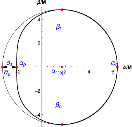
For calculating these parameters, we consider five points. The four points $\left(\alpha_{t},\beta_{t}\right),\left(\alpha_{b},\beta_{b}\right),\left(\alpha_{r},0\right)$ and $\left(\alpha_{p},0\right)$ are, respectively, the top, bottom, rightmost, and the leftmost point of the shadow; and $\left(\bar{\alpha}_{p},0\right)$ is the leftmost point of the reference circle. From simple geometry, we have expressions for the radius $R_{s}$ and the deviation from circularity $\delta_{s}$ as follows

$$R_{s}=\frac{\left(\alpha_{t}-\alpha_{r}\right)^{2}+\beta_{t}^{2}}{2\left(-\alpha_{t}+\alpha_{r}\right)},$$

(26)

and

$$\delta_{s}=\frac{\left(-\bar{\alpha}_{p}+\alpha_{p}\right)}{R_{s}}.$$

(27)

For all subsequent plots, we have taken $\theta=\pi/2$.

Here, we have given in a tabular form the deviation of the image $\delta_{s}$ of the Kerr-Sen-like black hole for set of values of $k\equiv\{0,.01,.02\}$ corresponding to the set of values of $k\equiv\{-.2,0,.2\}$ with $a=b=0.2$ and $\theta=\frac{\pi}{2}$.

It is known that black holes emit radiation and consequently, the mass of the black hole decreases and the process continues until it collapses down completely SW. For various black holes, this emission rate has been studied in the articles WEI; GHOSH; GHOSH1. In OUR, we have studied the energy emission rate for Kerr-Sen-like black holes and studied the consequences of Lorentz violation effect $l$ on it. Here we would like to study the energy emission in presence of plasma following the motivation from the article GHOSH1. The energy emission rate of radiation with the frequency $\omega$ is given by

$$\frac{d^{2}E}{d\omega dt}=\frac{2\pi^{3}R_{s}^{2}}{e^{\frac{\omega}{T}}-1}\omega^{3}.$$

(28)

where $\omega$ is the frequency and $T$ is the Hawking temperature given by OUR

$\displaystyle T=\frac{\sqrt{\left(2M-b\right)^{2}-4a^{2}\left(1+l\right)}}{4\pi M\sqrt{1+l}\left(2M-b+\sqrt{\left(2M-b\right)^{2}-4a^{2}\left(1+l\right)}\right)}.$

(29)

In WEI, it was conjectured that the black hole shadow corresponds to its high energy absorption cross-section for the observer located at infinity. In general, the absorption cross-section oscillates around a limiting constant value $\sigma_{lim}=\pi R^{2}_{s}$ for a spherically symmetric black hole WEI; MASH; MISNER. The reader may see the articles MASH; MISNER where it was shown that $\sigma_{lim}$ was proportional to the geometrical cross-section of its photon sphere. The fluctuation around the limiting value was also studied in FLUC. In GHOSH, it has been applied for studying energy emission. In GHOSH1, it was extended for the black hole in presence of plasma. Therefore, the energy emission rate is directly proportional to the surface area of the black hole, which may be considered to be approximately equal to the surface area of the shadow $S\approx\pi R_{s}^{2}$. Computing $R_{s}$ using the expression (26) and using (29) we can calculate the rate of emission of radiation, which enables us to plot energy emission versus frequency of radiation curve. In Fig. 16, we have studied how the energy emission rate will behave with the variation of the parameters $b$, $l$, and $k$. It is observed that the rate of emission is higher for smaller values of $b$. However, the reverse is the case when $k$ increases. It is evident from the spectrum that in the absence of plasma the minimum energy will be released from the black hole, which indeed agrees with the Kerr-Newman black hole BABAR. From the plots, we see that for negative $l$ there is an enhancement of emission whereas, for increasing positive value of $l$, there is a reduction in the emission of radiation.

The deflection of light or lensing in presence and in the absece of dispersive medium like plasma for different spacetime backgrounds has been studied in the earlier literature OY1; OY2; OY3; CARL; MFAT; GKV. The extension of it for this Kerr-Sen-like black hole is worth investigation. There is an LV parameter $l$. So from our study, the combined effect of the presence of plasma and Lorentz violation on the deflection of light can be estimated. To study it, weak field approximation will be useful. This approximation is given by the expression

$$g_{\mu\nu}=\eta_{\mu\nu}+h_{\mu\nu},$$

(30)

where $\eta_{\mu\nu}$ is the Minkowski metric and $h_{\mu\nu}$ is the perturbation metric over $\eta_{\mu\nu}$. The Minkowski metric $\eta_{\mu\nu}=diag(-1,1,1,1)$ and $h_{\mu\nu}$ has the the following properties under weak field approximation

	$\displaystyle h_{\mu\nu}\ll 1,\quad h_{\mu\nu}\rightarrow 0\quad under\quad x^{i}\rightarrow\infty,$
	$\displaystyle g^{\mu\nu}=\eta^{\mu\nu}-h^{\mu\nu},\quad h^{\mu\nu}=h_{\mu\nu}.$		(31)

Considering the weak plasma strength, the angle of deflection of photon propagating along $z$ direction under weak field approximation is given by WEAK

$$\hat{\alpha}_{k}=\frac{1}{2}\int_{-\infty}^{\infty}\left(h_{33}+\frac{h_{00}\omega^{2}-K_{e}N}{\omega^{2}-\omega_{e}^{2}}\right)_{,k}dz,$$

(32)

where $K_{e}=\frac{4\pi e^{2}}{m}$. For large r, the black hole metric can, approximately, be written down in the form

$$ds^{2}=ds_{0}^{2}+\left(\frac{2M}{r}-\frac{2Mb}{r^{2}}\right)dt^{2}+\left(1+l\right)\left(\frac{2M}{r}-\frac{2Mb}{r^{2}}\right)dr^{2},$$

(33)

where

$$ds_{0}^{2}=-dt^{2}+\left(1+l\right)dr^{2}+r^{2}\left(d\theta^{2}+\sin^{2}\theta d\phi^{2}\right).$$

(34)

The components $h_{\alpha\beta}$ in the Cartesian coordinates have the following expressions

	$\displaystyle h_{00}$	$\displaystyle=$	$\displaystyle\left(\frac{R_{g}}{r}-\frac{2Mb}{r^{2}}\right),$
	$\displaystyle h_{ik}$	$\displaystyle=$	$\displaystyle\left(1+l\right)\left(\frac{R_{g}}{r}-\frac{2Mb}{r^{2}}\right)n_{i}n_{k},$
	$\displaystyle h_{33}$	$\displaystyle=$	$\displaystyle\left(1+l\right)\left(\frac{R_{g}}{r}-\frac{2Mb}{r^{2}}\right)\cos^{2}\chi,$

where $R_{g}=2M$ and $\chi$ is the polar angle between 3-vector and z-axis. Using the above expressions in (32), the light deflection angle for a black hole sitting in plasma medium OY1; OY2; OY3; VS is given by

$$\hat{\alpha}_{p}=\frac{1}{2}\int_{-\infty}^{\infty}\frac{p}{r}\left(\frac{dh_{33}}{dr}+\frac{\omega^{2}}{\omega^{2}-\omega_{e}^{2}}\frac{dh_{00}}{dr}-\frac{K_{e}}{\omega^{2}-\omega_{e}^{2}}\frac{dN}{dr}\right)dz,$$

(35)

where $p^{2}=x_{1}^{2}+x_{2}^{2}$ refers to the impact parameter and $x_{1}$ and $x_{2}$ are the coordinates on the plane orthogonal to the $z$ axis. The expression of $r$ is $r=\sqrt{p^{2}+z^{2}}$. We have the relation for the frequency of photon

$$\omega^{2}=\frac{\omega_{\infty}^{2}}{\left(1-\frac{R_{g}}{r}+\frac{2Mb}{r^{2}}\right)}.$$

(36)

Here $\omega_{\infty}$ is the asymptotic value of photon frequency. After expanding in series on the powers of $\frac{1}{r}$, we can have the approximation

$$\left(1-\frac{\omega_{e}^{2}}{\omega^{2}}\right)^{-1}\simeq 1+\frac{4\pi e^{2}N_{0}r_{0}}{m\omega_{\infty}^{2}r}-\frac{4\pi e^{2}N_{0}r_{0}R_{g}}{m\omega_{\infty}^{2}r^{2}}.$$

(37)

Using this approximation, one can find the deflection angle $\hat{\alpha}_{p}$ of the light around a black hole in presence of plasma in a straightforward manner

	$\displaystyle\hat{\alpha}_{p}$	$\displaystyle=$	$\displaystyle\left(1+l\right)\frac{2R_{g}}{p}+\frac{2R_{g}}{p}\left(1+\frac{\pi^{2}e^{2}N_{0}r_{0}}{m\omega_{\infty}^{2}p}-\frac{4\pi e^{2}N_{0}r_{0}R_{g}}{m\omega_{\infty}^{2}p^{2}}\right)$		(39)
			$\displaystyle-\frac{2Mb}{4p^{2}}\left(3\pi+\frac{4\pi e^{2}N_{0}r_{0}}{m\omega_{\infty}^{2}p}\left(8-\frac{3\pi R_{g}}{p}\right)\right).$

We get $\hat{\alpha}_{p}=(1+l)\frac{2R_{q}}{p}$ in the absence of charge and plasma for the Schwarzschild black hole. The dependence of the angle of deflection $\hat{\alpha}_{p}$ on the impact parameter $p$ for various charge and plasma parameters are demonstrated in the figures below where $F=\frac{4\pi e^{2}N_{0}r_{0}}{m\omega_{\infty}^{2}}$. In the left panel, it is found that as the value of $b$ increases the angle of deflection decreases and it is seen that $\hat{\alpha}_{p}$ is maximum when $b=0.$ We also observe that the deflection angle $\hat{\alpha}_{p}$ increases with the increase in the plasma parameter (right panel). We also notice that the deviation of photons is smaller when the plasma factor is removed from the black hole background. It is also observed that the deflection angle increases with an increase in the value of the Lorentz violating parameter $l$.

We compare the shadows produced, from numerical calculations, by the Kerr-Sen-like black holes with the observed one for the $\mathrm{M}87^{*}$ black hole. For comparison we consider the experimentally obtained astronomical data for the circularity deviation $\Delta\leq 0.10$ and angular diameter $\theta_{d}=42\pm 3\mu as$ EHT1. The boundary of the shadow is described by the polar coordinate $(R(\phi),\phi)$ with the origin at the center of the shadow $(\alpha_{C},\beta_{C})$ where $\alpha_{C}=\frac{|\alpha_{max}+\alpha_{min}|}{2}$ and $\beta_{C}=0$.

If a point $(\alpha,\beta)$ over the boundary of the image subtends an angle $\phi$ on the $\alpha$ axis at the geometric center, $\left(\alpha_{C},0\right)$ and $R(\phi)$ be the distance between the point $(\alpha,\beta)$ and $\left(\alpha_{C},0\right)$, then the average radius $R_{\text{avg}}$ of the image is given by CBK

$$R_{\text{avg}}^{2}\equiv\frac{1}{2\pi}\int_{0}^{2\pi}d\phi R^{2}(\phi),\\$$

(40)

where $R(\phi)\equiv\sqrt{\left(\alpha(\phi)-\alpha_{C}\right)^{2}+\beta(\phi)^{2}}$, and $\phi=tan^{-1}\frac{\beta(\phi)}{\alpha(\phi)-\alpha_{C}}$.

With the above inputs, the deviation from circularity $\Delta C$ is defined by TJDP,

$$\Delta C\equiv 2\sqrt{\frac{1}{2\pi}\int_{0}^{2\pi}d\phi\left(R(\phi)-R_{\text{avg }}\right)^{2}}.$$

(41)

We also consider the shadow angular diameter which is define by

$$\theta_{d}=\frac{2}{d}\sqrt{\frac{A}{\pi}}$$

(42)

where $A=2\int_{r_{-}}^{r_{+}}\beta d\alpha$ is the shadow area and $d=16.8Mpc$ is the distance of $M87^{*}$ from the earth. These relations will enable us to accomplish a comparison between the theoretical predictions for Kerr-Sen-like black-hole shadows and the experimental findings of the Event Horizon Telescope collaboration.
Figures below represent the deviation from circularity $\Delta C$ as it is obtained for Kerr-Sen-like black holes for the angles of inclinations $\theta=90^{o}$ and $17^{o}$ respectively.

Figures below represent the angular diameter $\theta_{d}$ as it is obtained for Kerr-Sen-like black holes for the angles of inclinations $\theta=90^{o}$ and $17^{o}$ respectively.

For this type of estimation, a prerequisite independent input is the knowledge of the black hole mass, which is the intrinsic yardstick for this system. In the case of $\mathrm{M}87^{*}$, the mass has been estimated to be $M=(6.6\pm 0.4)\times 10^{9}M_{\odot}$ MASS. Considering $M=6.5\times 10^{9}M_{\odot}$ for the $\mathrm{M}87^{*}$ black hole, we use the observed value of deviation from circularity $\Delta C\leq 0.10$ as deduced by the EHT collaboration EHT1 in order to constrain the Kerr-Sen-like black hole parameters. We have made an attempt to put constraints on $(a,k)$, $(a,b)$ and $(a,l)$ by fixing the values of ($b,l$), ($k,l$) and ($b,k$) respectively. From Fig. 18 and Fig. 19, it is clear that over a finite parameter space, black hole shadows satisfy the bound $\Delta C\leq 0.10$. Fig. 20 and Fig. 21 reveal that the condition $\Delta C\leq 0.10$ is satisfied by the Kerr-Sen-like black hole in presence of plasma for the entire parameter space. From Fig. 22, Fig. 23 and Fig.24 it is clear that, for finite parameter space, angular diameters are within $1\sigma$ region i.e $\theta_{d}=39\mu as$. From figures above we can also conclude that for fixed values of black hole parameters, the apparent shadow circularity deviation and angular diameter decrease as the observer moves away from the equatorial plane toward the polar axis.

We may put constrain on the value of $l$ as well. By modelling M$87^{*}$ black hole as Kerr black hole, the author has found a lower limit a $a$ for the M$87^{*}$ black hole RODRIGO. If we bring this result under consideration in the present situation the interval of interest for $a$ becomes $[0.50M,0.99M]$ with $b=k=0$. Now if we combine the constraints $\Delta C\leq 0.10$ and $\theta_{d}=42\pm 3\mu as$ and the knowledge that $a\in[0.50M,0.99M]$, we observe that $l\in(-1,0.621031]$. Here we find upper bound of $l$ to be 0.621031, however $l$ cannot be equal to $-1$. So $l>-1$. So to consider both the positive and negative value of $l$ in every plot make sense and well justified

We have considered the Kerr-Sen-like black hole, which is a solution of Einstein-bumblebee gravity. It contains an LV parameter $l$. We study the propagation of light in a non-magnetized pressure-less plasma on this Kerr-Sen-like spacetime. We have considered the plasma as a medium with dispersive properties given by a frequency-dependent index of refraction. The gravitational field is determined by the mass, the spin, and the bumblebee parameter. The Gravitational field due to plasma is neglected here. We have studied how the nature of shadows gets affected by the LV effect associated with the bumblebee field in the pressure-less nonmagnetic plasma. We have also studied the energy emission scenario and the weak field lensing in the Kerr-Sen-like spacetime due to Einstein-bumblebee gravity background when it is veiled in a plasma medium. The results for Kerr, Kerr-like, and the Schwarzschild black holes can, as well, be obtained from this result with a suitable limit. We have investigated in detail the impact of the charge ($Q^{2}\propto b$), plasma parameter $k$, and the Lorentz violating bumblebee parameter $l$ on the structure of shadow, on the lensing effect of light, and on the energy emission due to black hole radiation. It has been found that the new parameters quantitatively influence the structure of the event horizon by altering the radius significantly. It is observed that the size of the shadow viewed by a distant observer reduces with an increase in the charge $Q$ and the size of the shadow appears to be larger with the increase in the plasma parameter $k$ in the presence of a bumblebee field.

Therefore, the bumblebee field maintains its action of deforming the shadow in presence of plasma. Since the energy liberated from the black hole depends on the area of the shadow, the rate of energy emission from the black hole is higher when the black hole is surrounded by a plasma. As far as the angle of deflection is concerned, the photons are observed to experience an increase in the deviation as the plasma factor $k$ increases. While on the other hand, the angle of deflection reduces sufficiently when the amount of charge parameter increases. It is also observed that the deflection angle increases with an increase in the value of the LV parameter $l$. Sufficient negative $l$ may cease the lensing effect too!

The theory of General Relativity predicts that the Kerr metric is capable of describing astrophysical black holes. However, such black holes may not exist in a perfect vacuum due to the presence of surrounding matter, like plasma, dark matter, etc. The accretion disks may also alter the black hole, which may not fit with the Kerr metric. The bumblebee modified Kerr spacetime enables the incorporation of potential deviations from the Kerr metric through the additional deviation parameters. The advantage of this type of modified gravity is that it is a generic one and it has the ability to cover the prediction of the Kerr metric since the introduced parameters can be chosen in such a way that it makes the null deviation of the shadow from Kerr spacetime. There is the theoretical motivation for modified theories of gravity indeed.

The EHT collaboration has captured the image of supermassive black hole $\mathrm{M}87^{*}$ exhibiting a deviation from circularity $\Delta C\leq 0.10$. The observation did not say anything about modified theories of gravity or suggest any alternatives to the Kerr black hole. Motivated by this, we considered Kerr-Sen-like modified black holes, which have additional deviation parameters $l$ and $b$ to the Kerr black hole. The presence of Plasma adds an additional parameter. We use the deviation from circularity $\Delta C\leq 0.10$ as deduced by the EHT collaboration to constrain the Kerr-Sen-like black hole parameters. We have observed that over a finite parameter space, black hole shadows satisfy the bound $\Delta C\leq 0.10$ both in the presence of plasma and in the absence of it.

Besides the result of the article RODRIGO allows us to put put constrain on the value of $l$. We have found that the value of the parameter $l>-1$ and the upper bound of it is 0.621031. So $l$ can take both positive and negative values.

Finally, we would like to mention that in the calculation of the rate of energy emission we did not consider the greybody factor. The mathematical formulation of it is much involved for any black hole and it is important if a quantitative estimation is attempted. Unfortunately, there is no available data to compare it with the real situation. A theoretical evaluation of it for this black hole may be done, which we are leaving for a separate study.

References

- (1) B. P. Abbott et al., Phys. Rev. Lett. 116, 061102 (2016).
- (2) K. Akiyama et al. (Event Horizon Telescope Collaboration), First M87 Event Horizon Telescope results. I. The shadow of the supermassive black hole, Astrophys. J. 875, L1 (2019).
- (3) K. Akiyama et al. (Event Horizon Telescope Collaboration), First M87 Event Horizon Telescope results. II. Array and instrumentation, Astrophys. J. 875, L2 (2019).
- (4) K. Akiyama et al. (Event Horizon Telescope Collaboration), First M87 Event Horizon Telescope results. III. Data processing and calibration, Astrophys. J. 875, L3 (2019).
- (5) K. Akiyama et al. (Event Horizon Telescope Collaboration), First M87 Event Horizon Telescope results. IV. Imaging the central supermassive black hole, Astrophys. J. 875, L4 (2019).
- (6) K. Akiyama et al. (Event Horizon Telescope Collaboration), First M87 Event Horizon Telescope results. V. Physical origin of the asymmetric ring, Astrophys. J. 875, L5 (2019).
- (7) K. Akiyama et al. (Event Horizon Telescope Collaboration), First M87 Event Horizon Telescope results. VI. The shadow and mass of the central black hole, Astrophys. J. 875, L6 (2019).
- (8) J. L. Synge: Mon. Not. R. Astron. Soc. 131 463 (1966).
- (9) K. Hioki and K. I. Maeda, Phys. Rev. D 80, 024042 (2009)
- (10) L. Amarilla, E. F. Eiroa and G. Giribet: Phys. Rev. D. 81 124045 (2010).
- (11) F. Atamurotov, B. Ahmedovand A. Abdujabbarov: Phys. Rev. D. 88 064004 (2013)
- (12) S. W. Wei and Y. X. Liu, J. Cosmol. Astropart. Phys. 11 (2013) 063.
- (13) A. Abdujabbarov, F. Atamurotov, Y. Kucukakca, B. Ahmedov, U. Camci, Astrophys. Space Sci. 344 429. (2013)
- (14) F. Atamurotov, A. Abdujabbarov and B. Ahmedov, Astrophys. Space Sci. 348 179 (2013)
- (15) U. Papnoi, F. Atamurotov, S. G. Ghosh and B. Ahmedov:Phys. Rev. D. 90 024073 (2014)
- (16) A. Grenzebach, V. Perlick and C. l. Nammerzahl, Phys. Rev. D. 89 124004 (2014)
- (17) Z. Li and C. Bambi, Journal of Cosmology and Astroparticle Physics, 2014 041 (2014).
- (18) Z. Stuchlik, D. Charbulak, J. Schee Eur.Phys. J. C78 180 (2018)
- (19) M. Ghasemi-Nodehi, Z. Li and C. Bambi, Eur. Phys. J. C. 75 (2015)
- (20) A. Abdujabbarov, M. Amir, B. Ahmedov and S. G. Ghosh, Phys. Rev. D. 93 104004 (2016)
- (21) F. Atamurotov, S. G. Ghosh, B. Ahmedov: Eur. Phys. J. C. 76 (2016)
- (22) G. S. Bisnovatyi-Kogan and O. Y. Tsupko: Phys. Rev. D. 98 084020 (2018)
- (23) R. Kumar, S. G. Ghosh, A. Wang, Phys. Rev. D. 100 124024 (2019)
- (24) S.W. Wei, Y.X. Liu, R. B. Mann: Phys. Rev. D. 99 041303 (2019)
- (25) M. Khodadi, A. Allahyari, S. Vagnozzi, D. F. Mota:JCAP 2009 026 (2020)
- (26) M. Khodadi, A. Allahyari, S. Vagnozzi, D. F. Mota:JCAP 2002 003 (2020)
- (27) D. O. Muhleman, I. D. Johnston, Phys. Rev. Lett. 17, 455 (1966)
- (28) D. O. Muhleman, R. D. Ekers, E. D. Fomalont, Phys. Rev. Lett. 24, 1377 (1970)
- (29) G. S. Bisnovatyi-Kogan and O. Y. Tsupko: Mon. Not. R. Astron. Soc. 404 1790 (2010)
- (30) O. Y. Tsupko and G. S. Bisnovatyi-Kogan: Gravit. Cosmol. 18 117 (2012)
- (31) O. Y. Tsupko and G. S. Bisnovatyi-Kogan, Gravit. Cosmol. 20 220 (2014)
- (32) V. Morozova, B. Ahmedov, A. Tursunov, Astrophys. Space. Sci. 346 513 (2013)
- (33) G. S. Bisnovatyi-Kogan and O. Y. Tsupko: Universe. 3 1 (2017).
- (34) A. Abdujabbarov, B. Toshmatov, J. Schee, Z. Stuchlyk B. Ahmedov: Int. J. Mod. Phys. D26 1741011 (2017).
- (35) A. Abdujabbarov, B. Ahmedov, N. Dadhich, F. Atamurotov: Phys. Rev. D96 (2017) 084017.
- (36) C. A. Benavides-Gallego, A. A. Abdujabbarov, C. Bambi: Eur. Phys. J. C78 (2018) 694.
- (37) V. Perlick, O. Y. Tsupko, G. S. Bisnovatyi-Kogan: Phys. Rev. D92 104031 (2015)
- (38) F. Atamurotov, B. Ahmedovand A. Abdujabbarov Phys. Rev. D 92 084005 (2015)
- (39) V.Perlick, O. Yu. Tsupko: Phys. Rev. D 95, 104003 (2017)
- (40) G. Z. Babarr, A. Z. Babar, F. Atamurotov: Eur.Phys.J. C80 761 (2020)
- (41) V. A. Kostelecky and S. Samuel: Phys. Rev. Lett. 63, 224 (1989)
- (42) V. A. Kostelecky and S. Samuel: Phys. Rev. D 39, 683 (1989);
- (43) V. A. Kostelecky and S. Samuel: Phys. Rev. D 40, 1886 (1989)
- (44) D. Colladay and V. A. Kostelecky, Phys. Rev. D 55, 6760 (1997).
- (45) D. Colladay, V.A. Kostelecky, Phys. Rev. D 55, 6760 (1997)
- (46) D. Colladay, V.A. Kostelecky, Phys. Rev. D 58, 116002 (1998)
- (47) V.A. Kostelecky, Phys. Rev. D 69, 105009 (2004)
- (48) R. Casana, A. Cavalcante, F. P. Poulis, E. B. Santos: Phys. Rev. D 97, 104001 (2018)
- (49) C. Ding, C. Liu, R. Casana, A. Cavalcante: Eur. Phys. J. C80, 178 (2020)
- (50) S. K. Jha, A. Rahaman: Eur.Phys.J. C81 345 (2021)
- (51) A. Sen: Phys.Rev.Lett.69,1006 (1992)
- (52) P. V. P. Cunha, C. A. R. Herdeiro, E. Radu Phys. Rev. Lett. 123, 1 011101, 2019,
- (53) D. Psaltis, et al, Event Horizon Telescope, Phys. Rev. Lett. 125, 14 141104, 2020,
- (54) N, Ashish, S. Mohanty, and A. Kumar, arXiv:2002.12786, 2020
- (55) S. H. Volkel, E. Barausse, N. Franchini, A. E. Broderick arXiv:2011.06812, 2020
- (56) K. Glampedakis, G. Pappas arXiv:2102.13573, 2021
- (57) M. Afrin, R. Kumar, S. G. Ghosh: MNRAS 504 5927 (2021)
- (58) S. U. Islam, S. G. Ghosh arXiv:2102.08289
- (59) Z. Li, A. Ovgun: Phys. Rev. D 101, 024040 (2020)
- (60) J. L. Synge Relativity: The General Theory. North-Holland, Amsterdam, 196
- (61) A. Abdujabbarov, B. Toshmatov, Z. Stuchlk and B. Ahmedov, arXiv:1512.05206
- (62) A. Rogers, Mon. Not. Roy. Astron. Soc. 451 17 (2015).
- (63) S. Dastan, R. Saffari, S. Soroushfar: arXiv:1610.09477
- (64) S. Hawking: Commun. Math. Phys. 43 199, (1975)
- (65) S.-W. Wei and Y.-X. Liu, J. Cosmol. Astropart. Phys. 11 063 (2013).
- (66) U. Papnoi, F. Atamurotov, S. G. Ghosh, B. Ahmedov: Phys. Rev. D 90, 024073 (2014).
- (67) A. Abdujabbarov, M. Amir, B. Ahmedov, S. G. Ghosh: Phys. Rev. D 93, 104004 (2016)
- (68) B. Mashhoon, Phys. Rev. D7 (1973) 2807
- (69) C.W. Misner, K.S. Thorne and J.A. Wheeler, Gravitation, Freeman, San Francisco (1973).
- (70) Y. Decanini, G. Esposito-Fareseand, A. Folacci, Phys. Rev. D 83 (2011) 044032
- (71) O. Y. Tsupko and G. S. Bisnovatyi-Kogan, Gravitation and Cosmology 20, 220 (2014).
- (72) O. Y. Tsupko and G. S. Bisnovatyi-Kogan, Gravitation and Cosmology 18, 117 (2012).
- (73) O. Y. Tsupko and G. S. Bisnovatyi-Kogan, Gravitation and Cosmology 15, 184 (2009).
- (74) Carlos A. Benavides-Gallego, A. A. Abdujabbarov, Cosimo Bambi: Eur. Phys. J. C78 694 (2018)
- (75) M. Fathi, M. Olivares, J.R. Villanueva, Eur.Phys.J C81 987 (2021)
- (76) G. V. Kraniotis: Gen.Rel.Grav. 46 1818 (2014)
- (77) A. Abdujabbarov, B. Toshmatov, J. Schee, Z. Stuchlik, B. Ahmedov, Int. J. Mod. Phys. D26 1741011 (2017).
- (78) V. S. Morozova, B. J. Ahmedov and A. A. Tursunov, Astrophys. Space Sci. 346, 513 (2013).
- (79) T. Johannsen and D. Psaltis, Astrophys. J. 718, 446 (2010).
- (80) Cosimo Bambi, Katherine Freese, Sunny Vagnozzi and Luca Visinelli, Phys.Rev.D100(4):044057(2019).
- (81) K. Gebhardt, J. Adams, D. Richstone, T. R. Lauer, S. M. Faber, K. Gultekin, J. Murphy, S. Tremaine: Astrophys.J. 729, 119 (2011)
- (82) R. Nemmen: Astrophys J. Letts L26 880 (2019)