Convolutional Hough Matching Networks

The Hough transform is a powerful detection method for a geometric object, which exploits the duality between parts and parameters of the object [1, 22]. It performs voting in a parameter space of the target object, called the Hough space, where votes from the object parts are accumulated to form local maxima in the space. The objects are then detected simply by identifying the positions of local maxima. The Hough matching method [6], inspired by the Hough transform, detects reliable correspondences by geometric voting from candidate matches. Given two images, it constructs the Hough space of parameters of geometric transformation between the two images and then accumulates votes of candidate matches for plausible transformation.

Let us assume a local region $\mathbf{x}$ on an image, that is represented by its geometric attributes, \ie, pose and shape. In principle $\mathbf{x}$ can be a form of any parameterization, but in this work we simply describe the region $\mathbf{x}$ by its center and scale. Now let us consider two images, $I$ and $I^{\prime}$, and two sets of local regions, $\mathcal{X}$ and $\mathcal{X}^{\prime}$, obtained from the two images, respectively. For any two regions $(\mathbf{x},\mathbf{x}^{\prime})\in\mathcal{X}\times\mathcal{X}^{\prime}$, a correlation function $c$ computes a non-negative similarity $c(\mathbf{x},\mathbf{x}^{\prime})$ using appearance features of the regions. The main idea of Hough matching is to create the Hough space $\mathcal{H}$, that is the space of all possible offsets $\mathbf{h}$ between two regions, \ie, translation and scaling, and accumulate votes from candidate matches onto the Hough space as

where $\|\cdot\|_{\mathrm{g}}$ represents a group-wise distance function that computes the distances separately for two groups, center and scale, \ie, $\|\mathbf{x}\|_{\mathrm{g}}=[\|\mathbf{x}_{\mathrm{xy}}\|;\|\mathbf{x}_{\mathrm{s}}\|]$ (subscripts $\mathrm{xy}$ for center and $\mathrm{s}$ for scale) and $k_{\text{iso}}$ is a kernel function that computes similarity between the observed offset, $\mathbf{x}^{\prime}-\mathbf{x}$, and the given offset $\mathbf{h}$ in the Hough space.¹¹ 1 For the kernel function, previous work uses a form of discretized Gaussian [6] or Dirac delta [20] without learning the kernel parameters. The kernel $k_{\text{iso}}$ is designed to assign a voting weight for each candidate match according to how close the offset induced by the match $(\mathbf{x},\mathbf{x}^{\prime})$ is to $\mathbf{h}$; we use the group-wise distance to differentiate the effects of center and scale in the kernel. The resultant voting map $v(\mathbf{h})$ over the Hough space $\mathcal{H}$ can be used to find reliable matches $(\mathbf{x},\mathbf{x}^{\prime})$ by suppressing spurious ones corresponding to relatively low voting scores $v(\mathbf{x}^{\prime}-\mathbf{x})$, \eg, updating the match score via $c(\mathbf{x},\mathbf{x}^{\prime})v(\mathbf{x}^{\prime}-\mathbf{x})$ [20]. Despite its good empirical performance [6, 18, 19, 20, 37, 42, 45, 47, 58], the global voting map $v(\mathbf{h})$, which is shared for all candidate matches, is limited in the sense that it cannot capture the reliability of a specific candidate match. This global position-invariant Hough space makes the output less accurate and weak to background clutter, \eg, increasing the score of distant outliers that has a similar offset to that of dominant inliers.

As illustrated in Fig. 2, in order to address the issue, we create a local and individual voting space for each candidate match $(\mathbf{x},\mathbf{x}^{\prime})$ by introducing local windows around the regions, $\mathbf{x}$ and $\mathbf{x}^{\prime}$:

where $\mathcal{P}(\mathbf{x})$ denotes the set of neighbor regions within the local window centered on $\mathbf{x}$. Since this local voting space is now dedicated to $(\mathbf{x},\mathbf{x}^{\prime})$, we can simply assign a match score $v$ for the candidate match by taking the vote value at the bin with offset zero:

With a slight abuse of notation, let us use $k(\mathbf{z},\mathbf{z}^{\prime})$ to represent the kernel value corresponding to two positions, $\mathbf{z}$ and $\mathbf{z}^{\prime}$, each representing a local region in the parameter space of regions, \ie, 3D space of center and scale in our case. The equation above then can be generalized to a form of 6D convolution with an arbitrary kernel $k$:

which becomes equivalent to Eq. 3 when the group-wise isotropic kernel $k_{\text{iso}}$ is used.

Note that this convolutional extension of Hough matching has a generic form; it reduces to a similar form of 4D convolutions in [26, 40, 54, 61] when the Hough space is restricted to center translation, and generalizes to higher dimensions beyond 6D when additional transformation dimensions is introduced such as rotation, shear, and others.

We design the convolutional Hough matching (CHM) as a learnable convolution layer:

where $b$ is a bias term for the layer and $k$ represents a kernel with a specific type of weight sharing. The group-wise isotropic kernel $k_{\text{iso}}$, which is directly derived from Hough matching, can be implemented by weight sharing among parameters with the same offset $|\mathbf{z}-\mathbf{z}^{\prime}|$ in $k(\mathbf{z},\mathbf{z}^{\prime})$. While it is a reasonable choice, the fully isotropic kernel assigns the same importance to the matches of the same offset regardless of their distances from the kernel position $(\mathbf{x},\mathbf{x}^{\prime})$. It may be an excessive constraint in the sense that the distance of an object from the center of focus is likely to be relevant to the importance.

We thus relax the isotropy and propose the position-sensitive isotropic kernel $k_{\text{psi}}(\|\mathbf{p}^{\prime}-\mathbf{p}\|_{\mathrm{g}};\|\mathbf{p}-\mathbf{x}\|_{\mathrm{g}},\|\mathbf{p}^{\prime}-\mathbf{x}^{\prime}\|_{\mathrm{g}})$ that differentiates the distances from the kernel position, $\|\mathbf{p}-\mathbf{x}\|_{\mathrm{g}}$ and $\|\mathbf{p}^{\prime}-\mathbf{x}^{\prime}\|_{\mathrm{g}}$. The kernel $k_{\text{psi}}$ is implemented by sharing parameters whose triplets, $(\|\mathbf{p}^{\prime}-\mathbf{p}\|_{\mathrm{g}},\|\mathbf{p}-\mathbf{x}\|_{\mathrm{g}},\|\mathbf{p}^{\prime}-\mathbf{x}^{\prime}\|_{\mathrm{g}})$, are the same.

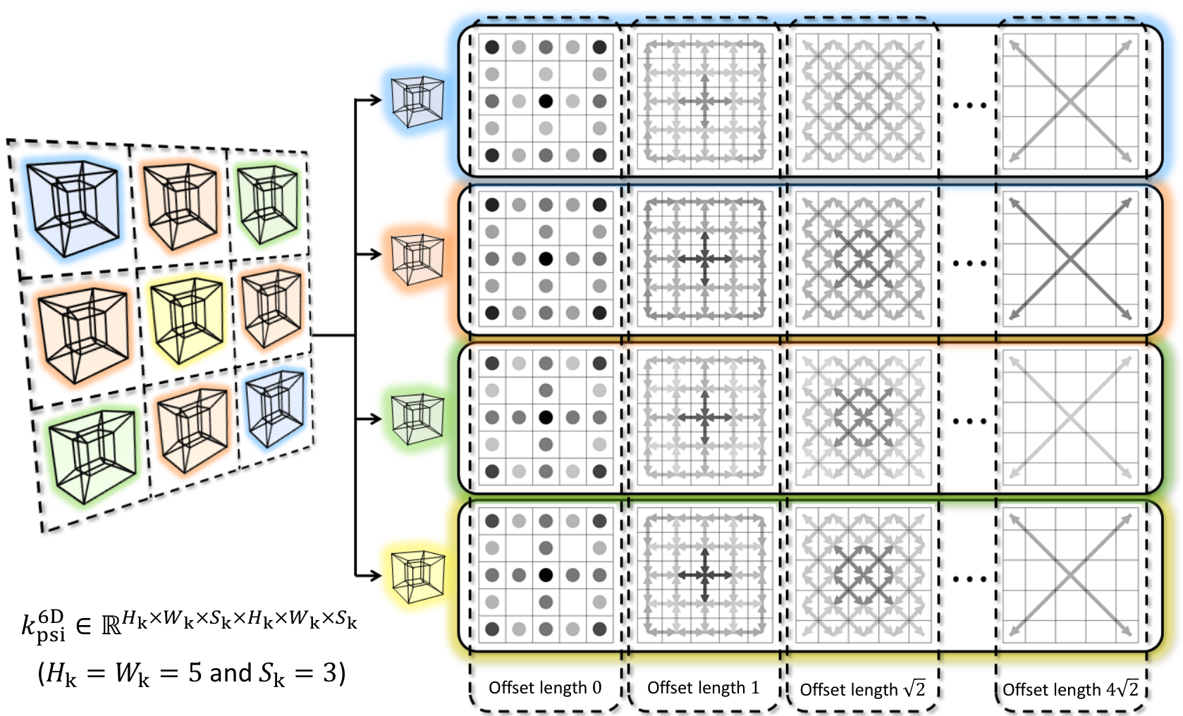
The CHM layer is compatible with any neural network layer that computes correlations between images, and can be stacked multiple times to improve the performance. As a result of substantial parameter sharing, the 6D kernels, $k_{\text{iso}}^{\mathrm{6D}}$ and $k_{\text{psi}}^{\mathrm{6D}}$ in $\mathbb{R}^{H_{\mathrm{k}}\times W_{\mathrm{k}}\times S_{\mathrm{k}}\times H_{\mathrm{k}}\times W_{\mathrm{k}}\times S_{\mathrm{k}}}$, contain only a small number of parameters, thus making CHM resistant to overfitting in training; \eg, the kernels with $H_{\mathrm{k}}=W_{\mathrm{k}}=5$ and $S_{\mathrm{k}}=3$ contains only 45 and 220 parameters, respectively, while the full kernel has 5,625. More importantly, the perspective of Hough matching on convolution provides the interpretability of the learned kernel: each element in the kernel is a voting weight of the corresponding neighbor match in the local offset space. Based on this perspective, Figure 3 visualizes the kernel $k_{\text{psi}}^{\mathrm{6D}}\in\mathbb{R}^{H_{\mathrm{k}}\times W_{\mathrm{k}}\times S_{\mathrm{k}}\times H_{\mathrm{k}}\times W_{\mathrm{k}}\times S_{\mathrm{k}}}$ of size $H_{\mathrm{k}}=W_{\mathrm{k}}=5$ and $S_{\mathrm{k}}=3$ trained in our experiment. For the ease of visualizing 6D tensor, we decompose it into multiple (four in case of $k_{\text{psi}}^{\mathrm{6D}}$) 4D tensors in which each of the map shows parameter values of the kernel with the same offset, where the arrows represent the offset vectors relative to the kernel position $(\mathbf{x},\mathbf{x}^{\prime})$, and the circles mean zero offset. The maps reveal that weights for matches with smaller offsets and closer distance are learned to be higher (darker), which appears to be a reasonable voting strategy. For more information, refer to our Appendix.

Following other recent methods [26, 40, 45, 47, 54], we also use as a CNN feature extractor pretrained on ImageNet classification [12]. Given an input image $I$, the feature extractor outputs a feature map in $\mathbb{R}^{C\times H\times W}$. We construct feature maps of multiple scales $\{{\mathbf{F}}_{s}\}_{s=1}^{S}$ by resizing the output for $S-1$ times by the scaling factor of $\sqrt{2}$, followed by $3\times 3$ conv layers with parameters $\{\theta_{s}\}_{s=1}^{S}$, reducing channel dimensions of input feature map by $1/\rho$. The $S$ different conv layers learn to capture effective semantic information of receptive fields with different scales for the subsequent multi-scale (6D) correlation computation. The same is done for $\{{\mathbf{F}}^{\prime}_{s}\}_{s=1}^{S}$ given image $I^{\prime}$. We set $S=3$, \ie, $\{1/\sqrt{2},1,\sqrt{2}\}$, and $\rho=4$ in our experiments.

Given a set of feature pairs from multiple scales $\{({\mathbf{F}}_{s},{\mathbf{F}}^{\prime}_{s})\}_{s=1}^{S}$, we compute all possible 4D correlation tensors placed on the $S\times S$ grid:

where $\mathbf{x}_{m}\in\mathcal{X}_{m}$ and $\mathbf{x}^{\prime}_{n}\in\mathcal{X}^{\prime}_{n}$ are spatial positions of feature map at scale $m$ and $n$, respectively, and ReLU clamps negative correlation scores to zero. To process it in the subsequent 6D CHM layer, we interpolate each 4D correlation $\mathbf{C}^{(0)}_{ij}$ to have the same spatial size to build 6D correlation tensor $\mathbf{C}^{\mathrm{(1)}}\in\mathbb{R}^{H\times W\times S\times H\times W\times S}$ such that ${\mathbf{C}}_{::i::j}^{\mathrm{(1)}}=\zeta_{1}({\mathbf{C}}_{ij}^{\mathrm{(0)}})$ where $\zeta_{1}(\cdot)$ is a function that interpolates input 4D tensor to the size ${H\times W\times H\times W}$.

A CHM layer takes the 6D correlation tensor ${\mathbf{C}}^{\mathrm{(1)}}$ to perform convolutional Hough voting in the space of translation and scaling: ${\mathbf{C}}^{\mathrm{(2)}}=\text{CHM}({\mathbf{C}}^{\mathrm{(1)}};k_{\mathrm{psi}}^{\mathrm{6D}})$, where $k_{\mathrm{psi}}^{\mathrm{6D}}\in\mathbb{R}^{H_{\mathrm{k}}\times W_{\mathrm{k}}\times S_{\mathrm{k}}\times H_{\mathrm{k}}\times W_{\mathrm{k}}\times S_{\mathrm{k}}}$ is a 6D position-sensitive isotropic kernel. In our experiments, we set $H_{\mathrm{k}}=W_{\mathrm{k}}=5$ and $S_{\mathrm{k}}=3$ with stride 1 for all dimensions and use zero-padding to the input to retain the same size at the output. We then perform max-pooling on ${\mathbf{C}}^{\mathrm{(2)}}$ to select the most dominant vote among candidate match scores in the scale space, reducing the tensor dimension down to 4D: ${\mathbf{C}}_{ijkl}^{\mathrm{(3)}}=\max_{m,n}{\mathbf{C}}_{ijmkln}^{\mathrm{(2)}}$. We proceed another CHM with a 4D kernel $k_{\mathrm{psi}}^{\mathrm{4D}}\in\mathbb{R}^{H_{\mathrm{k}}\times W_{\mathrm{k}}\times H_{\mathrm{k}}\times W_{\mathrm{k}}}$: ${\mathbf{C}}=\text{CHM}(\zeta_{2}(\sigma({\mathbf{C}}^{\mathrm{(3)}}));k_{\mathrm{psi}}^{\mathrm{4D}})$, where $\sigma(\cdot)$ is the sigmoid activation function and $\zeta_{2}(\cdot)$ is the upsampling function that resizes input 4D tensor to the size of $\bar{H}\times\bar{W}\times\bar{H}\times\bar{W}$ for fine-grained localization. We set $\bar{H}=2H$ and $\bar{W}=2W$ in our experiment.

We assume that keypoint match annotations are given for each training image pair, as in [9, 20, 40, 45, 47]; each image pair is annotated with a set of coordinate pairs $\mathcal{M}=\{(\mathbf{k}_{m},\mathbf{k}^{\prime}_{m})\}_{m=1}^{M}$, where $M$ is the number of annotations. Following the aforementioned keypoint transfer scheme, we obtain a set of predicted and ground-truth keypoint pairs on image $I^{\prime}$: $\{(\hat{\mathbf{k}}_{m}^{\prime},\mathbf{k}_{m}^{\prime})\}_{m=1}^{M}$ by assigning a match $\hat{\mathbf{k}}_{m}^{\prime}$ to each $\mathbf{k}_{m}$. Our objective in training is formulated as $\mathcal{L}=\frac{1}{M}\sum_{m=1}^{M}\|\hat{\mathbf{k}}_{m}^{\prime}-\mathbf{k}_{m}^{\prime}\|$, which minimizes the average Euclidean distance between the predicted keypoints and the ground-truth ones.

On the SPair-71k dataset, following [45, 47], we evaluate two versions for each model: a finetuned model (F), which is trained on SPair-71k, and a transferred model (T), which is trained on PF-PASCAL. On PF-PASCAL and PF-WILLOW, following the common evaluation protocol [9, 20, 26, 31, 40, 45, 47, 52, 54], our network is trained on the training split of PF-PASCAL [19] and evaluated on the test splits of PF-PASCAL and PF-WILLOW. We use the same training, validation, and test splits of PF-PASCAL used in [20]. The quantitative results are summarized in Tab. 1; we note different levels of supervision for each method in the first column to ensure fair comparison. The proposed model finetuned on SPair-71k (F) clearly surpass current state of the art by a significant margin, outperforming [47] by 9%p of PCK ($\alpha_{\mathrm{bbox}}=0.1$), \ie, 24.1% relative improvement. On PF-PASCAL, our model achieves 4.4%p and 0.9%p improvement with $\alpha_{\mathrm{img}}\in\{0.05,0.1\}$. Robust performance on SPair-71k (T) and PF-WILLOW verifies reliable transferability of our model. Figure 6 visualizes example qualitative results on SPair-71k.

Figure 5 plots precision-recall curves for the recent methods [40, 45, 47, 54] and ours. The proposed method clearly outperforms other methods, indicating our model effectively discriminates between semantic parts and background clutters as seen in the last row of Fig. 8 which visualizes sample pairs with top 300 confident matches. When CHM is either removed (w/o CHM) or replaced with global matching module (CHM $\xrightarrow{}$ RHM), predicted matches become unreliable, being mostly scattered on the background and even hardly regularized. For our model evaluated on SPair-71k, precision and recall have inverse relationship in most cases. Although initial growth in our PR curves on SPair-71k indicates that some true matches have in fact low match scores, it still surpasses the other models, revealing the reliability of our approach under large variations.

In Figure 7, we also plot frequencies over the maxpooled positions in scale-space after 6D CHM layer ($k_{\mathrm{psi}}^{\text{6D-4D}}$). The maximum votes on both PF-PASCAL and PF-WILLOW are mostly concentrated on the center scale whereas they are distributed over different scales on SPair-71k; this is a reasonable voting strategy as objects in PF-PASCAL and PF-WILLOW hardly vary in scale while those in SPair-71k show large variations in both scale and view-point.

These experiments imply that the high-dimensional convolution on a correlation tensor may play a different role from 2D convolution on an image feature tensor; the role of convolutional matching is to learn a reliable voting strategy rather than to capture diverse patterns in the correlation tensor. This is consistent with the Hough matching perspective, but previous 4D convolution methods [26, 40, 54, 61] with a different perspective commonly use multiple full kernels ($k_{\mathrm{full}}^{\mathrm{4D}}$) for layers. To verify our result, we have conducted a similar experiment using the model of [54] and obtained the consistent result; the original model, which uses channel sizes of $\{16,16,1\}$ for three layers of 4D convolution, achieves 76.2% PCK on our machine while the model with reduced channels of $\{1,1,1\}$ achieves 76.4% PCK. Note that in terms of the number of parameters in a layer, our CHM layers ($k^{\text{6D-4D}}_{\mathrm{psi}}$) have $247\sim 654$ times smaller number of parameters than the 4D convolution layers used in previous methods [26, 40, 54, 61]. This light-weight layer design is particularly important in practice, since the use of multiple channels, \iekernels, for high-dim convolution quickly increases the cost both in computation and memory.

For additional results and analyses, we refer the readers to the Appendix.

References

- [1] Dana H. Ballard. Generalizing the hough transform to detect arbitrary shapes. Pattern Recognition, 13, 1981.
- [2] Herbert Bay, Tinne Tuytelaars, and Luc Van Gool. Surf: Speeded up robust features. In Proc. European Conference on Computer Vision (ECCV), 2006.
- [3] Hilton Bristow, Jack Valmadre, and Simon Lucey. Dense semantic correspondence where every pixel is a classifier. In Proc. IEEE International Conference on Computer Vision (ICCV), 2015.
- [4] Hsin-Yi Chen, Yen-Yu Lin, and Bing-Yu Chen. Robust feature matching with alternate hough and inverted hough transforms. In Proc. IEEE Conference on Computer Vision and Pattern Recognition (CVPR), 2013.
- [5] Minsu Cho, Karteek Alahari, and Jean Ponce. Learning graphs to match. In Proc. IEEE International Conference on Computer Vision (ICCV), 2013.
- [6] Minsu Cho, Suha Kwak, Cordelia Schmid, and Jean Ponce. Unsupervised object discovery and localization in the wild: Part-based matching with bottom-up region proposals. In Proc. IEEE Conference on Computer Vision and Pattern Recognition (CVPR), 2015.
- [7] Minsu Cho, Jungmin Lee, and Kyoung Mu Lee. Reweighted random walks for graph matching. In Proc. European Conference on Computer Vision (ECCV), 2010.
- [8] Minsu Cho and Kyoung Mu Lee. Progressive graph matching: Making a move of graphs via probabilistic voting. In Proc. IEEE Conference on Computer Vision and Pattern Recognition (CVPR), 2012.
- [9] Christopher Choy, JunYoung Gwak, Silvio Savarese, and Manmohan Chandraker. Universal correspondence network. In Advances in Neural Information Processing Systems (NeurIPS), 2016.
- [10] Christopher Choy, Jaesik Park, and Vladlen Koltun. Fully convolutional geometric features. In Proc. IEEE International Conference on Computer Vision (ICCV), 2019.
- [11] Navneet Dalal and Bill Triggs. Histograms of oriented gradients for human detection. In Proc. IEEE Conference on Computer Vision and Pattern Recognition (CVPR), 2005.
- [12] Jia Deng, Wei Dong, Richard Socher, Li-Jia Li, Kai Li, and Li Fei-Fei. Imagenet: A large-scale hierarchical image database. In Proc. IEEE Conference on Computer Vision and Pattern Recognition (CVPR), 2009.
- [13] Gianluca Donato and Serge Belongie. Approximate thin plate spline mappings. In Proc. European Conference on Computer Vision (ECCV), 2002.
- [14] Matthias Fey, Jan E. Lenssen, Christopher Morris, Jonathan Masci, and Nils M. Kriege. Deep graph matching consensus. In International Conference on Learning Representations (ICLR), 2020.
- [15] Martin Fischler and Robert Bolles. Random sample consensus: A paradigm for model fitting with applications to image analysis and automated cartography. Communications of the ACM, 1981.
- [16] David Forsyth and Jean Ponce. Computer Vision: A Modern Approach. (Second edition). Prentice Hall, Nov. 2011.
- [17] Juergen Gall and Victor Lempitsky. Class-specific hough forests for object detection. In Proc. IEEE Conference on Computer Vision and Pattern Recognition (CVPR), 2009.
- [18] Bumsub Ham, Minsu Cho, Cordelia Schmid, and Jean Ponce. Proposal flow. In Proc. IEEE Conference on Computer Vision and Pattern Recognition (CVPR), 2016.
- [19] Bumsub Ham, Minsu Cho, Cordelia Schmid, and Jean Ponce. Proposal flow: Semantic correspondences from object proposals. IEEE Transactions on Pattern Analysis and Machine Intelligence (TPAMI), 2018.
- [20] Kai Han, Rafael S Rezende, Bumsub Ham, Kwan-Yee K Wong, Minsu Cho, Cordelia Schmid, and Jean Ponce. Scnet: Learning semantic correspondence. In Proc. IEEE International Conference on Computer Vision (ICCV), 2017.
- [21] Kaiming He, Xiangyu Zhang, Shaoqing Ren, and Jian Sun. Deep residual learning for image recognition. In Proc. IEEE Conference on Computer Vision and Pattern Recognition (CVPR), 2016.
- [22] Paul V.C. Hough. Method and means for recognizing complex patterns. U.S. Patent, 3069654, 1962.
- [23] Jie Hu, Li Shen, and Gang Sun. Squeeze-and-excitation networks. In Proc. IEEE Conference on Computer Vision and Pattern Recognition (CVPR), 2018.
- [24] Li Huan, Qin Yujian, and Wang Li. Vehicle logo retrieval based on hough transform and deep learning. In Proc. IEEE International Conference on Computer Vision (ICCV), 2017.
- [25] Gao Huang*, Zhuang Liu*, Laurens van der Maaten, and Kilian Weinberger. Densely connected convolutional networks. In Proc. IEEE Conference on Computer Vision and Pattern Recognition (CVPR), 2017.
- [26] Shuaiyi Huang, Qiuyue Wang, Songyang Zhang, Shipeng Yan, and Xuming He. Dynamic context correspondence network for semantic alignment. In Proc. IEEE International Conference on Computer Vision (ICCV), 2019.
- [27] Sangryul Jeon, Seungryong Kim, Dongbo Min, and Kwanghoon Sohn. Parn: Pyramidal affine regression networks for dense semantic correspondence. In Proc. European Conference on Computer Vision (ECCV), 2018.
- [28] Sangryul Jeon, Dongbo Min, Seungryong Kim, Jihwan Choe, and Kwanghoon Sohn. Guided semantic flow. In Proc. European Conference on Computer Vision (ECCV), 2020.
- [29] Wadim Kehl, Fausto Milletari, Federico Tombari, Slobodan Ilic, and Nassir Navab. Deep learning of local rgb-d patches for 3d object detection and 6d pose estimation. In Proc. European Conference on Computer Vision (ECCV), 2016.
- [30] Jaechul Kim, Ce Liu, Fei Sha, and Kristen Grauman. Deformable spatial pyramid matching for fast dense correspondences. In Proc. IEEE Conference on Computer Vision and Pattern Recognition (CVPR), 2013.
- [31] Seungryong Kim, Stephen Lin, Sangryul Jeon, Dongbo Min, and Kwanghoon Sohn. Recurrent transformer networks for semantic correspondence. In Advances in Neural Information Processing Systems (NeurIPS), 2018.
- [32] Seungryong Kim, Dongbo Min, Stephen Lin, and Kwanghoon Sohn. Dctm: Discrete-continuous transformation matching for semantic flow. In Proc. IEEE International Conference on Computer Vision (ICCV), 2017.
- [33] Diederik P. Kingma and Jimmy Ba. Adam: A method for stochastic optimization. In International Conference on Learning Representations (ICLR), 2015.
- [34] Jan Knopp, Mukta Prasad, and Luc Van Gool. Scene cut: Class-specific object detection and segmentation in 3d scenes. International Conference on 3D Imaging, Modeling, Processing, Visualization and Transmission, 2011.
- [35] Jan Knopp, Mukta Prasad, and Luc Van Gool. Orientation invariant 3d object classification using hough transform based methods. In Proceedings of the ACM Workshop on 3D Object Retrieval, 2010.
- [36] Alex Krizhevsky, Ilya Sutskever, and Geoffrey E Hinton. Imagenet classification with deep convolutional neural networks. In Advances in Neural Information Processing Systems (NeurIPS), 2012.
- [37] Suha Kwak, Minsu Cho, Ivan Laptev, Jean Ponce, and Cordelia Schmid. Unsupervised object discovery and tracking in video collections. In Proc. IEEE International Conference on Computer Vision (ICCV), 2015.
- [38] Junghyup Lee, Dohyung Kim, Jean Ponce, and Bumsub Ham. Sfnet: Learning object-aware semantic correspondence. In Proc. IEEE Conference on Computer Vision and Pattern Recognition (CVPR), 2019.
- [39] Bastian Leibe and Bernt Schiele. Interleaved object categorization and segmentation. In Proc. British Machine Vision Conference (BMVC), 2003.
- [40] Shuda Li, Kai Han, Theo W. Costain, Henry Howard-Jenkins, and Victor Prisacariu. Correspondence networks with adaptive neighbourhood consensus. In Proc. IEEE Conference on Computer Vision and Pattern Recognition (CVPR), 2020.
- [41] Ce Liu, Jenny Yuen, and Antonio Torralba. Sift flow: Dense correspondence across scenes and its applications. IEEE Transactions on Pattern Analysis and Machine Intelligence (TPAMI), 2011.
- [42] Yanbin Liu, Linchao Zhu, Makoto Yamada, and Yi Yang. Semantic correspondence as an optimal transport problem. In Proc. IEEE Conference on Computer Vision and Pattern Recognition (CVPR), 2020.
- [43] David G. Lowe. Distinctive image features from scale-invariant keypoints. International Journal of Computer Vision (IJCV), 2004.
- [44] Fausto Milletari, Seyed-Ahmad Ahmadi, Christine Kroll, Annika Plate, Verena Rozanski, Juliana Maiostre, Johannes Levin, Olaf Dietrich, Birgit Ertl-Wagner, Kai Bötzel, and Nassir Navab. Hough-cnn: Deep learning for segmentation of deep brain regions in mri and ultrasound. Computer Vision and Image Understanding, 2017.
- [45] Juhong Min, Jongmin Lee, Jean Ponce, and Minsu Cho. Hyperpixel flow: Semantic correspondence with multi-layer neural features. In Proc. IEEE International Conference on Computer Vision (ICCV), 2019.
- [46] Juhong Min, Jongmin Lee, Jean Ponce, and Minsu Cho. SPair-71k: A large-scale benchmark for semantic correspondence. arXiv prepreint arXiv:1908.10543, 2019.
- [47] Juhong Min, Jongmin Lee, Jean Ponce, and Minsu Cho. Learning to compose hypercolumns for visual correspondence. In Proc. European Conference on Computer Vision (ECCV), 2020.
- [48] David Novotny, Samuel Albanie, Diane Larlus, and Andrea Vedaldi. Semi-convolutional operators for instance segmentation. In Proc. European Conference on Computer Vision (ECCV), 2018.
- [49] Adam Paszke, Sam Gross, Francisco Massa, Adam Lerer, James Bradbury, Gregory Chanan, Trevor Killeen, Zeming Lin, Natalia Gimelshein, Luca Antiga, Alban Desmaison, Andreas Kopf, Edward Yang, Zachary DeVito, Martin Raison, Alykhan Tejani, Sasank Chilamkurthy, Benoit Steiner, Lu Fang, Junjie Bai, and Soumith Chintala. Pytorch: An imperative style, high-performance deep learning library. In Advances in Neural Information Processing Systems (NeurIPS). 2019.
- [50] Charles R. Qi, Or Litany, Kaiming He, and Leonidas J. Guibas. Deep hough voting for 3d object detection in point clouds. In Proc. IEEE International Conference on Computer Vision (ICCV), 2019.
- [51] Ignacio Rocco, Relja Arandjelovic, and Josef Sivic. Convolutional neural network architecture for geometric matching. In Proc. IEEE Conference on Computer Vision and Pattern Recognition (CVPR), 2017.
- [52] Ignacio Rocco, Relja Arandjelović, and Josef Sivic. End-to-end weakly-supervised semantic alignment. In Proc. IEEE Conference on Computer Vision and Pattern Recognition (CVPR), 2018.
- [53] Ignacio Rocco, Relja Arandjelović, and Josef Sivic. Efficient neighbourhood consensus networks via submanifold sparse convolutions. In Proc. European Conference on Computer Vision (ECCV), 2020.
- [54] Ignacio Rocco, Mircea Cimpoi, Relja Arandjelović, Akihiko Torii, Tomas Pajdla, and Josef Sivic. Neighbourhood consensus networks. In Advances in Neural Information Processing Systems (NeurIPS), 2018.
- [55] Michal Rolínek, Paul Swoboda, Dominik Zietlow, Anselm Paulus, Vít Musil, and Georg Martius. Deep graph matching via blackbox differentiation of combinatorial solvers. In Proc. European Conference on Computer Vision (ECCV), 2020.
- [56] Paul Hongsuck Seo, Jongmin Lee, Deunsol Jung, Bohyung Han, and Minsu Cho. Attentive semantic alignment with offset-aware correlation kernels. In Proc. European Conference on Computer Vision (ECCV), 2018.
- [57] Karen Simonyan and Andrew Zisserman. Very deep convolutional networks for large-scale image recognition. In International Conference on Learning Representations (ICLR), 2015.
- [58] Waqas Sultani and Mubarak Shah. What if we do not have multiple videos of the same action? — video action localization using web images. In Proc. IEEE Conference on Computer Vision and Pattern Recognition (CVPR), 2016.
- [59] Min Sun, Gary Bradski, Bing-Xin Xu, and Silvio Savarese. Depth-encoded hough voting for joint object detection and shape recovery. In Proc. European Conference on Computer Vision (ECCV), 2010.
- [60] Tatsunori Taniai, Sudipta N Sinha, and Yoichi Sato. Joint recovery of dense correspondence and cosegmentation in two images. In Proc. IEEE Conference on Computer Vision and Pattern Recognition (CVPR), 2016.
- [61] Prune Truong, Martin Danelljan, and Radu Timofte. GLU-Net: Global-local universal network for dense flow and correspondences. In Proc. IEEE Conference on Computer Vision and Pattern Recognition (CVPR), 2020.
- [62] Xiaolong Wang, Allan Jabri, and Alexei A. Efros. Learning correspondence from the cycle-consistency of time. In Proc. IEEE Conference on Computer Vision and Pattern Recognition (CVPR), 2019.
- [63] Fan Yang, Xin Li, Hong Cheng, Jianping Li, and Leiting Chen. Object-aware dense semantic correspondence. In Proc. IEEE Conference on Computer Vision and Pattern Recognition (CVPR), 2017.
Appendix A Additional results and analyses
Analysis on scale-space maxpool. To further analyze the results in Fig. 7, we visualize maxpooled positions of predicted matches on sample pairs of SPair-71k [46], PF-PASCAL [19], and PF-WILLOW [18]. Figure A3 shows the results and describes how we visualize them. Due to large scale-variations in pairs of SPair-71k, our model collects winners of scale-space vote, \ie, , from diverse positions in scale-space. In contrary, objects in PF-PASCAL and PF-WILLOW exhibit relatively small scale-variations, thus encouraging our model to collect winners of the vote mostly from the original scales. We observe that the maxpooled positions typically depend on scales of object’s parts as seen in Fig. A3.
Learned CHM kernels. Figure A4 describes how we visualized Fig. 3. For straightforward visualization of high-dimensional geometry on 2D plane, we use tesseracts and their arrangement on a 2D grid to represent 4D and 6D tensors respectively. Learned kernels of (ours), , and are respectively visualized in Figs A5, A6, and A7.
Interestingly, the weight patterns of kernels and are remarkably similar; the weights for matches with large offsets and closer distance are learned to be higher (darker) while those with small offsets and far distance are learned to be lower (brighter). Moreover, learned weight patterns of 4D maps in second, fourth, sixth, and eighth rows of in Fig. A6 are noticeably similar to each other. We also observe that patterns in first and last rows, and patterns in third and seventh rows of are similar to each other as well. In contrast, is unable to express diverse weight patterns due to its parameter-sharing constraint that enforces full isotropy. This observation reveals that our kernel in CHMNet clearly benefits from its reasonable parameter-sharing strategy, in terms of both efficiency and accuracy as demonstrated in Tab. 2.
Appendix B More implementation details
Coordinate normalization. Following the work of [38], we use height and width normalized coordinates to ensure numerical stability of loss gradients such that