On the Impulsive Heating of Quiet Solar CoronaJournal: ApJThe analysis was primarily performed in python, using the Tensorflow (Abadi et al. 2016) package for machine learning – data download alone was done using Solarsoft (Freeland & Handy 1998). Computational tools used were Numpy (Van Der Walt et al. 2011; Oliphant 2006; Harris et al. 2020), Scipy (Virtanen et al. 2020) and Astropy (Price-Whelan et al. 2018; Astropy Collaboration et al. 2013). Parallelization was performed using Multiprocessing (McKerns et al. 2012), and plotting using Matplotlib (Hunter 2007) and Seaborn (Waskom & the seaborn development team 2020). Most of the code has been written in Jupyter environment (Kluyver et al. 2016). The codebase is under expansion for future work, and shall be made available on request.
Abstract
The solar corona consists of a million-degree Kelvin plasma. A complete understanding of this phenomenon demands the study of Quiet Sun (QS) regions. In this work, we study QS regions in the 171 Å, 193 Å and 211 Å passbands of the Atmospheric Imaging Assembly (AIA) on board the Solar Dynamics Observatory (SDO), by combining the empirical impulsive heating forward model of Pauluhn & Solanki 2007 with a machine-learning inversion model that allows uncertainty quantification. We find that there are impulsive events per min, with a lifetime of about min. Moreover, for all the three passbands, the distribution of power law slope peaks above 2. Our exploration of correlations among the frequency of impulsive events and their timescales and peak energy suggests that conduction losses dominate over radiative cooling losses. All these finding suggest that impulsive heating is a viable heating mechanism in QS corona.
Keywords:
Sun, Corona, AtmosphereI Introduction
Full disk images of the Sun taken in extreme ultraviolet (EUV) and X-rays, consist of three features: Active Regions (ARs), Coronal holes (CHs), and Quiet Sun (QS). The ARs are the brightest, CHs appear darkest, whereas QS regions appear like a background. Note that while the number of ARs is a function of solar activity cycle, QS is present irrespective of the activity phase. There is a lot of literature studying the coronal heating in the ARs (see Reale 2014, for a review) – however, studies of coronal heating in QS and CHs are sparse (Tripathi et al. 2021, see e.g.). To address the physics of coronal heating in general, a comprehensive study of the heating in QS regions is of paramount importance(Aschwanden 2014).
One of the most popular mechanisms to heat the corona is via impulsive events , viz. Nanoflares (Parker 1988, see e.g.). Impulsive events are transients generated through the dissipation of magnetic stresses or waves (Antolin et al. 2008, see e.g.,). Solar atmosphere presents us with plethora of impulsive events at various energies and time scale, viz. flares (Benz 2008; Tripathi et al. 2004), microflares (Hannah et al. 2008; Schadee et al. 1983; Subramanian et al. 2018; Chifor et al. 2006; Chifor et al. 2007), active region transient brightenings (Testa et al. 2013; Gupta et al. 2018a; Tripathi 2021; Vilangot Nhalil et al. 2020; Rajhans et al. 2021), transition region blinkers (Harrison 1997), UV bombs (Peter et al. 2006; Gupta & Tripathi 2015), Ellerman bomb (Ellerman 1917; Pariat et al. 2004; Isobe et al. 2007) and other activities such as jets (Mulay et al. 2016; Raouafi et al. 2016). It is also observed that the properties of loops in ARs are well described by the impulsive heating scenario (Ghosh et al. 2017; Tripathi et al. 2009; Warren et al. 2008; Gupta & Tripathi 2015; Winebarger et al. 2013b, and references therein). Such a scenario has also been studied independently in ARs using a variety to techniques like Time lag analysis (Viall & Klimchuk 2012; Viall & Klimchuk 2013; Viall & Klimchuk 2015; Viall & Klimchuk 2016; Viall & Klimchuk 2017), Differential Emission Measure (DEM) and Doppler shifts analysis (Tripathi et al. 2010; Tripathi et al. 2011; Tripathi et al. 2012; Winebarger et al. 2011; Warren et al. 2012; Winebarger et al. 2013a; Subramanian et al. 2014; Del Zanna et al. 2015, see e.g.,), hydrodynamic modelling (Bradshaw et al. 2012; Reep et al. 2013; Cargill et al. 2015; Barnes et al. 2016, see e.g.), Magneto hydrodynamic modelling (Rappazzo 2015; Rappazzo et al. 2017; Knizhnik et al. 2018; Knizhnik et al. 2019; Knizhnik & Reep 2020, see e.g.) and empirical models (Jess et al. 2019; Jess et al. 2014, see eg.). Thus, it is natural to assume that the coronal heating in QS may also be governed by impulsive heating. However, since the QS regions have a very diffuse structure, it is not possible to count individual events and understand the energetics of these events in the QS.
To maintain the corona at a million degree, the frequency distribution of impulsive events must follow a power law distribution in energy – i.e., with (Hudson 1991, see). Observations do show that impulsive events in the corona follow a power-law distribution – however, there are a range of values reported in the literature (Aschwanden 2019, see, for example, Fig. 6.14 in).
One of the most significant caveats in these results is due to the assumption that the each detected event is a single entity. But, we know that small-scale impulsive events may happen at a sub-resolution scale. Hence, individual brightenings may not be single entity but may consist of many tiny events. This may lead to the under counting of events particularly at lower energies. Moreover, the observations of QS radiance in UV and EUV, both in space and time, show log-normal distribution (Pauluhn et al. 2001). Thus, the the QS radiance might be generated due to some form of a Markovian process (Pauluhn & Solanki 2007; Gorobets et al. 2016).
To mitigate the the above mentioned issues, Pauluhn & Solanki 2007 proposed an empirical model for the heating of the QS corona. Hereafter, we call it the Pauluhn and Solanki Model (PSM). In brief, PSM approximates the response of the plasma to a unit heating event as an exponential rise and fall of intensity. The amplitude of the heating event is sampled from a power-law distribution, with the frequency of occurrence of the events being kept as a free parameter. The resultant light curve is then a combination of a multitude of these events. Hence this addresses the sub-pixel resolution scale of these structures. Moreover, the resulting intensities are also shown to be log-normal, mimicking the observations. Finally, the observed power-law distribution of energetic events is also incorporated in this model, thereby enabling us to understand the viability of impulsive events maintaining the observed intensity in a given light curve. Thus, PSM may provide an excellent proxy for the generation of the QS coronal intensities.
Pauluhn & Solanki 2007 generate the parameters for different observations by comparing similarity of intensity distribution and the Global Morlét wavelet power (Torrence & Compo 1998) of simulated light curves with those of observed light curves. The comparison is qualitative – a sufficient good match in distribution, and the frequency location of peaks in the power spectrum were taken to represent a good match between the observation and simulation. Although the comparison had a sound basis, it was done by eye, and needs to be on a more quantitative foundation.
The problem of obtaining parameters from the observed light curve thus becomes an inversion problem. In general, the inversion approaches depend primarily on generating important “features” from the light curves which then have a one to one mapping with the parameter set of PSM. This is essentially performed qualitatively by Pauluhn & Solanki 2007. Since it is quite non trivial to objectively pick out features for inversion, one trains an inversion model to pick out abstract features, and perform the inversion. In this case, an optimization principle guides the mapping from light curves to parameter set developed by the inversion model.
Tajfirouze & Safari 2012; Bazarghan et al. 2008 employed this method by using a Probabilistic Neural Network (PNN). Under this scheme, every simulated light curve is classified, where each class has a unique combination of free parameters. The PNN is trained on the full set of simulated light curves. Finally, the observed light curves are fed into the PNN, which then assigns each of them to one of the learned classes. For their study, Tajfirouze & Safari 2012 used 10,000 light curves (at max). These light curves corresponded to CHs, QS, and ARs on the Sun obtained from the Atmospheric Imaging Assembly (Lemen et al. 2012, AIA;) on board Solar Dynamics Observatory (Pesnell et al. 2012, SDO;) and data from the Extreme UltraViolet Imager (EUVI) on board STEREO (Kaiser et al. 2008). On average, they obtained for all the regions.
This method is a great start to a tricky stochastic inversion problem. But, such an approach must be well-validated by an exhaustive testing set. Moreover, the classification of light curves imposes a discretisation constraint on the parameter set, which depends on the grid resolution of the simulation. Thus, any assigned class to a given light curve may change on improving the grid resolution. In other words, we do not know the confidence level of the PNN for each inversion.
We further emphasize that Tajfirouze & Safari 2012 used poor resolution of AIA 171 Å data (s cadence and ″spatial resolution), and further binned the data spatially by and window. Such a binning will average out the small scale events, and thus, will not allow the use of full potential of AIA observations. Here we use the full spatial and temporal resolution observations taken using AIA and perform a regression on the target parameter set using a Convolutional Neural Network (LeCun et al. 2015, CNN;), that circumvents the potential caveats in the work of Tajfirouze & Safari 2012; Bazarghan et al. 2008 as detailed above.
A CNN is used to preserve information of the time scales of features in the light curve along with the distribution of intensity values. A CNN may be thought of as a set of ‘kernels’, which perform convolution on the input and return a convolved output. The kernel size can be interpreted as the scale over which information is summarized. Several such kernels are operated on a given input, and these outputs are passed through a non-linear function called the ‘Activation function’. Successive kernels are thus sensitive to local scales of the corresponding input, but that input itself may be an extremely non-linear transformation of the original light curve.
Furthermore, we do not use a simple CNN for the inversion. Instead, we use an Inception module, which improves its performance (Szegedy et al. 2015, see,). The Inception module provides kernels with multiple sizes at the same level and makes is possible to perform multi-scale analysis at each level. By employing a CNN to capture the scales of variation present in the data, we circumvent grid resolution issues by considering the target as a regression problem. We can effectively interpolate between simulated grid points while performing the inversion. With the CNN, we also obtain associated inversion uncertainties by perturbing the network.
II Observations and Data
For this work, we have used the observations recorded by AIA onboard SDO. AIA observes the Sun’s atmosphere in UV and EUV bands using eight different passbands sensitive to plasma at different temperatures (O’Dwyer et al. 2010a; Boerner et al. 2012). Here we have used the data taken using 171 Å, 193 Å and 211 Å passbands. These images are taken with a pixel size of 0.6″ and an approximate time cadence of 12 s. We have chosen these particular passbands since the count rates in these passbands for QS is large, when compared to others (O’Dwyer et al. 2010b, see Table 2 in).
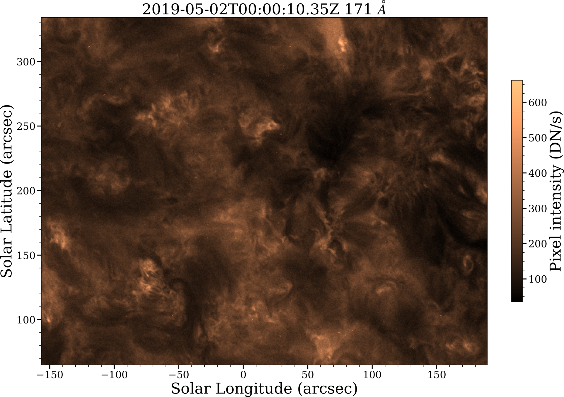
Monitoring the EUV images on Solar Monitor 11 1 https://www.solarmonitor.org/, we have identified QS patches during 2011 and 2019, where no activity was observed. Details of the two data sets (DS1 & DS2) are given in Table. 1. In total, we have obtained eight continuous hours of data for each set, which corresponds to 2400 time steps. All the images are aligned to the first image and are exposure time normalized. The full FOV (single snapshot) for DS1 and DS2 as observed in 171 Å is displayed in the left panel of Figs. 1 & 2 with the corresponding spatial distribution of intensities in the right panels.
| Identifier | DS 1 | DS 2 |
|---|---|---|
| Start time | 2011-08-14 T00:00:00 | 2019-05-02 T00:00:00 |
| End time | 2011-08-14 T08:00:00 | 2019-05-02 T08:00:00 |
| Reference time | 2011-08-14 T00:00:00 | 2019-05-02 T00:00:00 |
| Xcen,Ycen | 192″, 749″ | 19.0″, 211.5″ |
| FOVx, FOVy | 230″, 116″ | 346.0″, 269.0″ |
| Instrument | AIA | AIA |
| Passband | 171,193,211 | 171,193,211 |
| Exposure normalize | True | True |
| Cadence | 12 sec | 12 sec |

To study the distribution of the intensity, for each pixel we create light curves of intensity in all three passbands. We plot sample light curves from both the datasets, for one passband, and their corresponding distribution in Figs. 3 & 4 for a single pixel. Note that we also show time series of magnetic flux density of the corresponding pixel taken from the Helioseismic and Magnetic Imager (Scherrer et al. 2012, HMI; ) on board SDO corresponding to the AIA Field of View (FOV). The LOS magnetograms are obtained by HMI at approximately 45 s cadence with a pixel size of 0.5″. We map the HMI data to the same plate scale as that of AIA. The error in HMI LOS measurements is estimated to be 10G (Yeo et al. 2014; Couvidat et al. 2016), and this is depicted in the figure as the black horizontal line. The time series for intensity and magnetic flux density are shown in panels b and c. The distributions are shown in panels a and d, respectively, which demonstrate the log-normal distribution, as was previously observed by Pauluhn & Solanki 2007 in SUMER observations and Tajfirouze & Safari 2012 for AIA observations.
III Noise Characterization of the light curves
The observed light curves, shown in Figs. 3 and 4, have inherent noise, which is essentially dominated by photon shot noise. To mitigate this, while preventing over-smoothing (and thus averaging over real events), we use a procedure that we call Finding kneemo.
Finding kneemo is based on existing knee analyses performed in Machine learning. Broadly, the goal of the algorithm is to monitor a performance metric against the free parameter, which, in our case, is the size of the smoothing window. The window size for which we observe a drastic improvement in performance metric is taken as the box-car window. The change point is generally known as “the knee”.
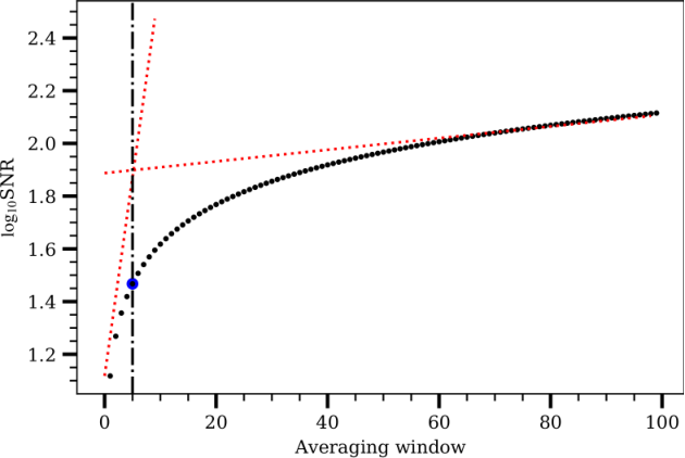
The knee determination is extremely qualitative, though some methods exist which quantify this well (Salvador & Chan 2004, see, for example). In our analysis, we consider a random light curve for a pixel in our data set, along with its error time series, which is obtained from aia_bp_estimate_error.pro. We smooth light curve using box-car of box size varying between 1 and 100, and obtain its modified SNR (Signal-to-Noise Ratio). We then plot the obtained SNR against the box size in Fig. 5, along with the asymptotes of the SNR, and find their point of intersection. This point is then selected as the box-car window size. From Fig. 5, we find that the asymptotes intersect at box-car size of 5 time-points. Therefore, we use this value to enhance SNR. Note that we have run this analysis on several lightcurve within our dataset and have found a consistent result. Thus, we have performed box-car averaging with box size of 5 time-points for all the light curves in our dataset. An example plot with the original and the smoothed light curve is shown in Fig. 6.
IV Methods
IV.1 Nanoflare model
The forward model employed here, as mentioned earlier, is the PSM. This is an empirical model based on two key observations, i.e. log-normal distribution of spatial and temporal distribution of QS intensities (Pauluhn et al. 2001), and power law distribution of energies from flares to micro-flares (Aschwanden 2019, see, e.g.). The algorithm may be summarised by asking the following questions:
- 1.
What is the probability of a flare to occur at a given time step?
- 2.
If a flare is meant to occur at the given time step, what would its peak energy be?
- 3.
How long will the flare last once it has occurred, i.e. the duration of the flare?
In this model there are 5 free parameters: the event or flaring frequency (), i.e., the probability of a flare to occur at a given time; the duration of the individual flare event (); the power law slope () and the minimum () and the maximum () energy that is allowed for an individual flare events, which provides the bounds of the power law. An example simulated light curve, depicting the formation of light curve from individual events is shown in Fig. 7. It may be seen from here that given only the envelope light curve, the individual events may not be inferred. We note that the simulations are performed over a large parameter space (see Table 2), while fixing and , to perform the inversion of light curves from all the three passbands with the same inversion model.
We generate the light curves for length of , where is the length of the light curve (2400 in our case), and reject 800 samples from either side to remove boundary effects. The remaining light curve is folded times to get a final light curve of length 22 2 Folding essentially divides up the light curve in 5 equal chunks of length L and gets the average curve from these chunks. This is done to minimize the effects of the initial seed for random number generators. The observed light curves are normalized by their median values, following Bazarghan et al. 2008. Hence, the radiances reported from hereon have no associated units.
| Parameter | Range | Stepsize |
|---|---|---|
| steps of 0.05 | ||
| steps of 0.1 | ||
| steps of 2.0 | ||
| 0.3 | ||
| 0.03 |
IV.2 Inversion
We perform the inversion using 1-D CNN. In this approach, generally, there are convolution layers followed by an activation layer. The activation, as we have seen in Sec. I, is a non-linear function which forms the core of complex learning ability of any NN. We use the function Elu as defined in Eqn IV.2 as activation for all layers except the last, since Elu enables the network to train faster and generalize better (Clevert et al. 2015). For the final layer, we have no activation since this is a regression problem mapping to a continuous variable.
A graphical representation of the model architecture is shown in Fig. 8. As depicted in the figure, there are input/output layers, convolution layers (where we implicitly assume the activation function to be present), and fully connected (FC) layers. In the tensor shape, ‘None’ is generally used to denote a variable size, which in this case represents number of light curves to be inverted during a single forward pass. The convolution layers (marked in red) are given a 4-dimensional shape, representing [height, width, input channel, output channel], and the stride size given by an integer. Note that “channel” here is not to be confused with AIA passbands, and that since we have used a 1-D signal, the height is set to 1. After a suitable number of convolutions, the array is unrolled to 1D, and captured by fully-connected layers (marked in yellow). For more information on general CNN and training see Goodfellow et al. 2016.

IV.3 Data preparation and training
We have divided the simulated light curves into training set (80%) and testing set (20%). However, before feeding in any data to the CNN, it must be prepared appropriately to make sure all the parameters are of the same scale. The training set parameters are rescaled between 0 and 1, and the testing set parameters are rescaled using the training statistics, as is the standard procedure in machine learning. All light curves are also rescaled between 0 and 1.
We train the CNN by feeding in the training set light curves, and obtain three free parameter set (, and ). This obtained parameter set is them compared with the original target parameter set using an error metric, which is used to update the kernel values of the CNN. The error metric is the sum of the two terms defined as:
| (4) |
where is the target parameter set, is the predicted parameter set, and the summation is performed over all observations, and all parameters.
There are certain “free parameters” that needs to be fixed while developing any NN. These free parameters are called hyper-parameters, while the trainable parameters of the NN are called the “weights” of the NN. For training the CNN, we have used the “Adam Optimizer” (Kingma & Ba 2014), which is a stochastic optimization algorithm. The “size” of update at each step is controlled by the hyper-parameter called learning rate.
Overfitting is a serious issue in NN training whereby the model starts fitting the noise in the model, and stops generalizing. This may result in erroneous results and interpretation of inversion. To prevent over fitting, we use dropout (Hinton et al. 2012), which essentially switches off neurons randomly with a fixed probability for every forward pass. The training hyper parameters are summarized in Table. 3.
| Hyperparameter | Value |
|---|---|
| Cost function | (prediction,target)+(prediction,target) |
| Optimizer | Adam Optimizer with default values |
| Learning rate | |
| Dropout rate | |
| No. of iterations |
IV.4 Uncertainty estimation
A CNN generates a single prediction for a given forward pass. However, in general, there exist two kinds of uncertainties – namely Epistemic and Aleatoric – associated with any such predictions (Kendall & Gal 2017). Epistemic uncertainty relates to model uncertainty due to unexplored weight space of the neural network. Aleatoric uncertainty relates to the inherent uncertainty in the target parameter values. In our study, there is no Aleatoric uncertainty because the parameters are defined by us. Hence, we have only Epistemic uncertainty.
Deficiencies in model training, resulting in unexplored weight space, can occur if not enough data is provided during model training. Hence, this effect can be simply minimized by increasing the size of training set. However, the epistemic uncertainty measure, while informing us about the deficiencies in fitting, may also inform us about any outliers in the dataset. Throughout the analysis in this work, the PSM is assumed to be the ground truth, i.e, it fully describes the observed light curves to infer parameters. This is obviously never the case with any model. Hence, departures of the observations from simulations, where the PSM does not fully explain the given observation, would behave as outliers. Hence higher uncertainties associated with the parameters inferred from the observations tells us either there are deficiencies in model fitting in certain regimes, or the light curve is not explained well by the PSM. However, we note that it is practically impossible to disentangle these effects (Kendall & Gal 2017, see e.g.,).
The epistemic uncertainty may be estimates by application of dropout (Hinton et al. 2012; Díaz Baso et al. 2019). In addition to being used to prevent overfitting, Dropout can also be used to create perturbations, and obtain the variability in the predictions (Gal 2016). Since the neurons switched off in every forward pass are random, we perform a Monte Carlo forward pass to obtain multiple realizations of the CNN, and present the mean, standard deviation from the passes. Thus, the error bars reported for the estimated parameters of an individual light curve are the standard deviation obtained from Dropout.
IV.5 Inversion performance


To asses the performance of our CNN, in Fig.9, we display scatter plots between the target and predicted values of (left panel), (middle panel) and (right panel). As can be readily noted, the predicted values lie very close to the target values, thereby validating the performance of our network on a test set. This may be quantified using the coefficient of determination () defined as:
| (5) |
where represents the mean of target set, represents the target values, and represents the predicted values. In this case, corresponds to number of points in the test set, i.e. is computed separately for each target parameter. The values are 0.990, 0.999 and 0.97 for , and , respectively, showing excellent performance of our network. Our network is now ready to be fed in with the observed intensity light curve.
V Results
Now we discuss the application of the network on the observed light curves. We first discuss the results obtained for a single light curve in §V.1. Then in §V.2, we move on to discuss the results obtained for all light curves obtained for all the three AIA passbands. We next explore the various correlations between our parameters and perform an analysis of the involved energetics in §V.3.
V.1 Application of the CNN on a Single Light curve
For representative purpose, we choose the intensity light curve for a random pixel from both DS1 and DS2 and obtain the corresponding simulated light curve. It is important to note that since PSM is a statistical model which generates a representation of the observations “statistically”, one should not perform a point by point comparison of the simulations with the observations. A simple change in the seed of the random number generator can change the exact times when events occur. Furthermore, since the amplitude of events is sampled from a distribution, the random seed value can also change the event amplitude at particular times. However, these seeds cannot change the overall statistical properties of the light curve. Thus, a comparison of the observation and simulation must be done using statistical properties of light curves (e.g intensity distribution, frequencies showing enhances power), rather than a pointwise comparison of light curves. Once a good representative simulated light curve is obtained, the corresponding parameter set is taken to characterise the observed light curve.
In Figs. 10 and 11, we show the comparison between observed (orange) and simulated (blue) light curves (panels a), Kernel Density Estimation (KDE) of intensity distribution (panels b), the Global Morlét power spectra (panels c) and the cumulative distribution function (CDF; panels d). Note that both the observed and simulated light curves are normalized by their median. The parameter sets denoted for the simulated light curves are the mean values of the obtained parameter distribution by performing 1000 Monte Carlo simulations, and are denoted at the bottom of the figures.The KDE can be understood to be essentially a continuous extension of histogram (Chen 2017, see eg.). Note that and are defined as per time step in Fig. 9, and may be converted into real units as
and
The denoted henceforth is given as number of events per minute, while is given as timescale in minutes. The remains a dimensionless parameter.
From panels a of Figs. 10 and 11, we can see an excellent statistical correspondence between the observed and simulated light curve. This is corroborated by the match in their corresponding KDEs (panel b) and CDFs (panel d). Furthermore, the Morlét wavelet power spectrum shows peaks at corresponding frequencies for both the observed and simulated light curve. These results confirm that the Inversion model was able to learn both the time series and distribution properties corresponding to the 3 free parameters. We further emphasize that value of inferred in these two cases is , which in turn suggests that events with smaller energy are dominantly responsible for generation of radiance of these particular examples.
From Figs. 10 and 11, we find a clear relation between the goodness of representation of simulated light curve (using CDF and Morlét Power) and the spread of parameters obtained by Monte Carlo simulations. Consider the percentage uncertainty (i.e, uncertainty/mean value) – we find this quantity is approximately in for DS1, in for DS2; in for DS1 and DS2; and for DS1 and for DS2. Thus, the Inversion model is more certain of the parameters of DS1 than DS2, which is also reflected in the relative mismatch of Morlét power between the observation and simulation for DS2 over DS1, at the first two peaks (note the difference in y-axis limits in panels c). Thus, such an uncertainty measure, along with the Monte Carlo forward pass, can help us explain which parameters are strongly influencing the quality of a given inversion assuming PSM as the ground truth.
V.2 Multi-light curve - multi-passband analysis
Since our network gives reliable results for the light curve obtained for a random pixel in both the data set, we now take all of our light curves ( light curves per passband), for the three AIA passbands, and pass them through the network to obtain the relevant parameter set for each light curve. Due to operational constraints, we perform only 100 Monte Carlo forward passes in this case. We emphasize that the obtained parameter set for 100 and 1000 Monte Carlo forward passes, are statistically same for a limited, handpicked set of representative light curves.
For both of our data set, we first divide each light curve by its median value, rescale between 0 and 1, perform the Monte Carlo forward pass through the CNN, and obtain the mean parameter set. Finally, we concatenate the parameter set across the whole field of view for both data set separately for each AIA passband to improve our statistics. This concatenation can be done since all light curves are from QS regions and are evolving independently. Fig.12 displays the distribution of flaring frequency (panel a), duration (panel b) and power-law slope (panel c) for this concatenated dataset. The solid blue curves are for 171 Å, dashed-dotted red for 193 Å and dashed green are for 211 Å observations.
The plots reveal that the distribution of all three parameters for all passbands are remarkably similar. The pf distribution peaks at events per minute for 171 Å and at 2.4 events per minute for 193 and 211 Å, with a range of values between 1 and 4 events per minute. The distribution of peaks near 12 minutes for 211 Å, 14 minutes for 193 Å and 16 minutes for 171 Å, implying a slight temperature dependence. However, we emphasize that since the AIA passbands are multi-thermal, this inference should be taken with caution.
The distribution of , plotted in panel c, ranges between to , with peak at for all three passbands. When we consider the whole set of light curves, we find that of light curves in Å have , while the fraction is and respectively for Å and 211 Å passbands respectively. Thus, we find a reduction in dominance of lesser energy events as we progressively probe the QS in hotter passbands. We also note that the fall-off for all the three parameters goes from the hotter passband (i.e. 211 Å) falling off first, followed by progressively cooler channels (193 and 171 Å respectively).
To further understand any peculiarities exhibited by the QS for the two domains of , we plot the variation of with in Fig. 13. To boost the SNR, we have averaged within a constant bin of . Note that the bin size for averaging is obtained from Doane 1976. The error bars shown are 3 standard error33 3 Standard error is defined as , where is the standard deviation in the sample present in the bin, and is the number of points in the sample. Following Pauluhn & Solanki 2007, the factor may be interpreted as the ratio of excitation (i.e, intensity generation by ) to damping (i.e, intensity dissipation by ) for a given pixel. Here, we investigate the dominance of one over the other.
The plot reveals that there is almost no change in the excitation to damping ratio for , and is independent of in this regime. However, for the dynamics changes, and we find a reduction in the ratio with increasing . The larger errorbars at the end are due to poor statistics. But even considering the variation till , we find a considerable reduction in the ratio with , presenting an increasing dominance of damping over excitation. Thus, there is either a reduction in excitation, or an increase in damping, or both, which comes into play once the smaller events start dominating radiance generation.
V.3 Energetics
With the parameter set obtained, we can now investigate the involved energetics. A simple way to understand the energetics is from comparing the behaviour of the slope vis-a-vis the other free parameters. A large slope implies a predominance of smaller energies, while a small slope implies predominance of larger energies.
To quantify relations in terms of the peak intensity of a nanoflare, Pauluhn & Solanki 2007 defined the average peak nanoflare radiance () as:
| (6) |
is a measure of the average peak nanoflare radiance value for a given time series. Using Eq. 6, we estimate the values of for each pixel, and study its relationship with flaring frequency () as well as flare duration (), through scatter plots between these parameters.
In Fig. 14, we plot (left panel) and (right panel) as a function of for all three wavelengths. Note that we have averaged the free parameters within a constant bin of , and our errorbars are standard errors.
The plots reveal a slight tendency of decreasing pf as function of Eavg, albeit there is sharp decline in the beginning. However, monotonically increases with increasing Eavg till about E and shows saturation thereafter. Moreover, the plot further suggests a systematic lowering of flaring duration, being largest for coolest passband (171 Å).
VI Summary, Discussion and Conclusion
QS coronal region provides a wealth of data to narrow down and understand the underlying heating processes. Assuming the underlying heating mechanism to be impulsive, coronal light curves may be approximated using empirical statistical models to infer physics-inspired parameters. To this end, we construct an inversion model of the PSM using CNN and validate it using a separate test set. We perform the inversion on two coronal datasets and infer the free parameters for the three AIA pass-bands viz. 171 Å, 193 Å and 211 Å.
We find that the light curves inverted using the CNN and observed light curves are statistically in excellent statistical agreement, considering the CDF and KDEs (see Fig. 10 & 11). Note that we are not concerned with a point-to-point match at each timestep between the simulation and the observation. A change in the seed of the random number generator is enough to shift the location of individual events and their amplitudes in simulation. However, this does not cause any changes in the statistical properties of the light curve, which is what we are primarily interested in. The Global wavelet power shows the simulations and observations to have peaks at similar frequencies, validating that the simulation and observation both have enhanced power in similar frequencies. The quality of approximation may be understood by the Epistemic uncertainty of our CNN, obtained by the application of Dropout to perturb the model.
We find the distribution of all parameters to be similar for light curves from all three passbands. The flaring frequency lies within the range of 1 to 4 events per minute, with a peak at events per minute for all three passbands. Similarly, the flaring duration has a range of values between 5 and 30 minutes. However, unlike the flaring frequency, the peak of the distribution of flaring duration shows temperature dependence, being highest (16 min) for coolest 171 Å channel, 14 min for 193 AA and lowest (12 min) for the hottest 211 AA channel.
The power-law index has a range of values between 1 and 8. The distribution of peaks at 2.3 for all three passbands of AIA viz. 171, 193, and 211 Å. This finding strongly suggests that nanoflare heating is indeed a viable source of energy in the quiet corona (Hudson 1991, see, e.g.,). We also find the fraction of light curves giving progressively reduces from cooler to hotter passbands. We further note that there are a significant number of pixels where . This is suggestive that low energy events may not be dominant everywhere. However, note that the viability of these low energy events also relies on the flaring frequency , requiring a full analysis of the energetics.
Our finding further suggests that there is a change of dynamics for pixels with and (from Fig. 13). In the former case, is nearly constant, while in the latter case, it reduces with increasing . This may also be observed in Fig. 14. Note that corresponds nearly to and the right tail of represents . Here, a definite increase of with decreasing is seen, which is interpreted as excitation increasing with decreasing (and thus increasing ). However, we also find that reduces with reducing . Thus, the increase in damping counters that in excitation in regime, causing a reduction in the ratio in Fig. 13. Thus, the increase is excitation is essentially nullified by the increase in damping.
We note that our inferred distribution peaks at events per minute, while Tajfirouze & Safari 2012 obtained a mean of 0.33 events per min. This may be explained by the better temporal cadence and spatial resolution of our data, whereby our simulation captures much smaller transient events. However, note that our inferred corresponds to an average waiting time of sec, which is much smaller than the waiting times of s suggested from simple geometric arguments (Klimchuk 2015).
There is a discrepancy in the (decay time) and derived here with those obtained by Tajfirouze & Safari 2012. The being about a factor of six smaller in our case ( min in Tajfirouze & Safari 2012 to 10 min in our case) and peaking near in our case, compared to a mean of 2.6 in Tajfirouze & Safari 2012. This discrepancy may be attributed to the fact that the data used in this study are at much higher spatial and temporal resolution than Tajfirouze & Safari 2012. Therefore, we must have captured smaller events with much shorter timescales (as also alluded to by Tajfirouze & Safari 2012). Similarly, the discrepancy in power-law index may be attributed to the high spatial resolution data used in the present work. Moreover, in our simulation, we are sampling flares within a larger energy range with larger than those by of Tajfirouze & Safari 2012). However, note that our obtained cooling time scales ( sec) are indeed of the order of cooling time scales in the corona obtained by Klimchuk 2015(sec).
Next, we find that the decreases with (see left panel in Fig. 14). The decrease of with is interpreted as a decrease in peak energy released per flare with increasing frequency. Thus, we can either have intermittent, high energy events or sustained low energy events. This variation of with is similar to the observation of the relation obtained between peak flare flux and waiting times by Hudson 2020 (Sarkar et al. 2019, see also). Furthermore, the inverse relation between and , (or a direct relation between the waiting time and succeeding nanoflare energy) was a necessary ingredient needed to reproduce observed EM distribution with temperature in ARs by Cargill 2014. Since the rise time is given as a fraction of the decay time in this setup, we do not distinguish between pre-flaring and post-flaring times. Thus, this may point to the presence of a reservoir of energy that may be exhausted by frequent, small-energy events or intermittent, large-energy events. However, we emphasize that the change in is tiny (2-3 events per min, as can be seen from Fig. 14) when compared to the total time scale of these events (10-15 min across all passbands). Thus, we must take this interpretation with caution.
The time scale is seen to increase with (see right panel in Fig. 14). This shows an increase in flare time scale corresponds to an increase in average flare energy. This weak correlation is similar to the weak correlation observed between peak flux and flare time scale by Veronig et al. 2002. However, we may seek to explain this relation qualitatively as below:
For an iso-thermal, optically thin plasma, the observed intensity is directly proportional to electron number density (O’Dwyer et al. 2010b), i.e . From Cargill 1994, we find that:
| (7) |
and
| (8) |
where and are conductive and radiative cooling times, respectively.
Combining the equations of timescale and intensity, we obtain:
| (9) |
Thus, for a conduction cooling dominated plasma, the timescale should increase with the emitted intensity, while for a radiative cooling dominated plasma, we expect the opposite. Our results show a direct relation between and the peak flare intensity and qualitatively suggest that in such events, conduction losses are dominant over radiative losses, assuming a constant flaring frequency. This is similar to the results obtained by Rajhans et al. 2021; Gupta et al. 2018b; Subramanian et al. 2018 for tiny transient brightenings.
Finally, the flaring time scales are seen to be largest in the coolest passband, and are seen to decrease from the cooler to hotter passbands. This indicates the decreasing dominance of conduction loss over radiative loss (but the conduction loss still dominates), as would be the case for cooling loops (Klimchuk 2006; Viall & Klimchuk 2012; Tripathi et al. 2009; Gupta et al. 2015, see e.g.,). We emphasize that this is true under the assumption of constant flaring frequency since only 2-3 events are happening per minute, whereas our total (rise+fall) time in consideration 15 min.
It is important to emphasize that the PSM is very well suited for explaining the observed light curves from the quiet Sun region obtained at much higher temporal and spatial resolution than was initially studied by Pauluhn & Solanki 2007. We note that although we have improved the inference by quantifying the uncertainties, the PSM may further be developed by incorporating the plasma filling factor and effective area in the forward model, as has also been suggested in the original paper (Pauluhn & Solanki 2007). Note that in the PSM, the radiance distribution is considered to be same as energy distribution. However, note that there may be a number of further smaller events which may or may not produce detectable signatures in the intensity images. It is also possible that many events produce signature in one passband, and not in another. Therefore the distribution reported using the radiance is just a lower limit of the total number of events. Hence, incorporation of filling factors in the PSM is an important next step in improving the model.
Moreover, note that we have fixed the , limiting the energy range considered for the simulation. Therefore, it would be prudent to keep this ratio as a variable quantity. We have tried to develop an inversion model with varying over three orders of magnitude – however, the inversion model did not give adequate performance (the for was on the testing set). Thus, introducing the radiance ratio as a free parameter creates a large degeneracy in parameter space (Pauluhn & Solanki 2007, already been hinted to by), which cannot be solved by our neural network or the optimization scheme. Hence, further modeling and training strategies are required to disentangle such highly degenerate parameter spaces. Furthermore, it has been reported that the distribution of flare waiting time (inverse of flaring frequency) follow a time-dependent Poisson process, which gives rise to a power law-tail of waiting time distributions (Wheatland & Litvinenko 2002). Thus, the assumption of a constant flaring frequency (which translates to exponential waiting time distribution) may also need to be revised in the PSM.
It is important to note that a lot of the magnetic field strength is below the 10 Gauss limit (see Figs. 10 & 11. However, the variability in the magnetic field strength suggests that the corona is extremely dynamic even in the quiet regions. Hence, for any study to characterize the heating of quiet corona, we need magnetic field measurement with much higher sensitivity and at greater resolution.
Finally, note that while our current analysis has been focused on the QS corona, Bazarghan et al. 2008 have applied PSM to AR corona successfully, although using data at a very low spatial and temporal resolution. Thus, we expect our results to also extend to AR corona. Furthermore, it would be interesting to apply our inversion model to chromospheric observations (Jess et al. 2014, see also). This may be performed on spectral lines with Interface Region Imaging Spectrograph (De Pontieu et al. 2014, IRIS), or using chromospheric observations in Near-UltraViolet (NUV) from the Solar Ultraviolet Imaging Telescope (Tripathi et al. 2017; Ghosh et al. 2016, SUIT;), onboard the Aditya-L1 mission (Seetha & Megala 2017) of Indian Space Research Organization (ISRO).
References
- Abadi et al. (2016) Abadi, M., Barham, P., Chen, J., et al. 2016, in 12th USENIX Symposium on Operating Systems Design and Implementation (OSDI 16), 265–283
- Antolin et al. (2008) Antolin, P., Shibata, K., Kudoh, T., Shiota, D., & Brooks, D. 2008, ApJ, 688, 669, doi: 10.1086/591998
- Aschwanden (2014) Aschwanden, M. J. 2014, in Encyclopedia of the Solar System (Third Edition), third edition edn., ed. T. Spohn, D. Breuer, & T. V. Johnson (Boston: Elsevier), 235 – 259, doi: https://doi.org/10.1016/B978-0-12-415845-0.00011-6
- Aschwanden (2019) —. 2019, The Quiet-Sun Corona (Cham: Springer International Publishing), 219–259, doi: 10.1007/978-3-030-13956-8_6
- Aschwanden (2019) Aschwanden, M. J. 2019, New Millennium Solar Physics, Vol. 458, doi: 10.1007/978-3-030-13956-8
- Astropy Collaboration et al. (2013) Astropy Collaboration, Robitaille, T. P., Tollerud, E. J., et al. 2013, A&A, 558, A33, doi: 10.1051/0004-6361/201322068
- Barnes et al. (2016) Barnes, W. T., Cargill, P. J., & Bradshaw, S. J. 2016, ApJ, 833, 217, doi: 10.3847/1538-4357/833/2/217
- Bazarghan et al. (2008) Bazarghan, M., Safari, H., Innes, D. E., Karami, E., & Solanki, S. K. 2008, A&A, 492, L13, doi: 10.1051/0004-6361:200810911
- Benz (2008) Benz, A. O. 2008, Living Reviews in Solar Physics, 5, 1, doi: 10.12942/lrsp-2008-1
- Boerner et al. (2012) Boerner, P., Edwards, C., Lemen, J., et al. 2012, Sol. Phys., 275, 41, doi: 10.1007/s11207-011-9804-8
- Bradshaw et al. (2012) Bradshaw, S. J., Klimchuk, J. A., & Reep, J. W. 2012, ApJ, 758, 53, doi: 10.1088/0004-637X/758/1/53
- Cargill (1994) Cargill, P. J. 1994, ApJ, 422, 381, doi: 10.1086/173733
- Cargill (2014) Cargill, P. J. 2014, The Astrophysical Journal, 784, 49, doi: 10.1088/0004-637x/784/1/49
- Cargill et al. (2015) Cargill, P. J., Warren, H. P., & Bradshaw, S. J. 2015, Philosophical Transactions of the Royal Society of London Series A, 373, 20140260, doi: 10.1098/rsta.2014.0260
- Chen (2017) Chen, Y.-C. 2017, A Tutorial on Kernel Density Estimation and Recent Advances. https://arxiv.org/abs/1704.03924
- Chifor et al. (2006) Chifor, C., Mason, H. E., Tripathi, D., Isobe, H., & Asai, A. 2006, A&A, 458, 965, doi: 10.1051/0004-6361:20065687
- Chifor et al. (2007) Chifor, C., Tripathi, D., Mason, H. E., & Dennis, B. R. 2007, A&A, 472, 967, doi: 10.1051/0004-6361:20077771
- Clevert et al. (2015) Clevert, D.-A., Unterthiner, T., & Hochreiter, S. 2015, arXiv preprint arXiv:1511.07289
- Couvidat et al. (2016) Couvidat, S., Schou, J., Hoeksema, J. T., et al. 2016, Sol. Phys., 291, 1887, doi: 10.1007/s11207-016-0957-3
- De Pontieu et al. (2014) De Pontieu, B., Lemen, J., Kushner, G., et al. 2014, Solar Physics, 289, 2733
- Del Zanna et al. (2015) Del Zanna, G., Tripathi, D., Mason, H., Subramanian, S., & O’Dwyer, B. 2015, A&A, 573, A104, doi: 10.1051/0004-6361/201424561
- Díaz Baso et al. (2019) Díaz Baso, C. J., de la Cruz Rodríguez, J., & Danilovic, S. 2019, A&A, 629, A99, doi: 10.1051/0004-6361/201936069
- Doane (1976) Doane, D. P. 1976, The American Statistician, 30, 181, doi: 10.1080/00031305.1976.10479172
- Ellerman (1917) Ellerman, F. 1917, ApJ, 46, 298, doi: 10.1086/142366
- Freeland & Handy (1998) Freeland, S. L., & Handy, B. 1998, Solar Physics, 182, 497
- Gal (2016) Gal, Y. 2016, University of Cambridge, 1
- Ghosh et al. (2017) Ghosh, A., Tripathi, D., Gupta, G. R., et al. 2017, ApJ, 835, 244, doi: 10.3847/1538-4357/835/2/244
- Ghosh et al. (2016) Ghosh, A., Chatterjee, S., Khan, A. R., et al. 2016, in Space Telescopes and Instrumentation 2016: Ultraviolet to Gamma Ray, Vol. 9905, International Society for Optics and Photonics, 990503
- Goodfellow et al. (2016) Goodfellow, I., Bengio, Y., & Courville, A. 2016, Deep Learning (MIT Press)
- Gorobets et al. (2016) Gorobets, A., Borrero, J., & Berdyugina, S. 2016, The Astrophysical Journal Letters, 825, L18
- Gupta et al. (2018a) Gupta, G. R., Sarkar, A., & Tripathi, D. 2018a, ApJ, 857, 137, doi: 10.3847/1538-4357/aab95e
- Gupta et al. (2018b) —. 2018b, ApJ, 857, 137, doi: 10.3847/1538-4357/aab95e
- Gupta & Tripathi (2015) Gupta, G. R., & Tripathi, D. 2015, ApJ, 809, 82, doi: 10.1088/0004-637X/809/1/82
- Gupta et al. (2015) Gupta, G. R., Tripathi, D., & Mason, H. E. 2015, ApJ, 800, 140, doi: 10.1088/0004-637X/800/2/140
- Hannah et al. (2008) Hannah, I. G., Christe, S., Krucker, S., et al. 2008, ApJ, 677, 704, doi: 10.1086/529012
- Harris et al. (2020) Harris, C. R., Millman, K. J., van der Walt, S. J., et al. 2020, Nature, 585, 357, doi: 10.1038/s41586-020-2649-2
- Harrison (1997) Harrison, R. A. 1997, Sol. Phys., 175, 467, doi: 10.1023/A:1004964707047
- Hinton et al. (2012) Hinton, G. E., Srivastava, N., Krizhevsky, A., Sutskever, I., & Salakhutdinov, R. R. 2012, arXiv preprint arXiv:1207.0580
- Hudson (1991) Hudson, H. 1991, Solar Physics, 133, 357
- Hudson (2020) Hudson, H. S. 2020, MNRAS, 491, 4435, doi: 10.1093/mnras/stz3121
- Hunter (2007) Hunter, J. D. 2007, Computing in Science & Engineering, 9, 90, doi: 10.1109/MCSE.2007.55
- Isobe et al. (2007) Isobe, H., Tripathi, D., & Archontis, V. 2007, ApJ, 657, L53, doi: 10.1086/512969
- Jess et al. (2014) Jess, D. B., Mathioudakis, M., & Keys, P. H. 2014, ApJ, 795, 172, doi: 10.1088/0004-637X/795/2/172
- Jess et al. (2019) Jess, D. B., Dillon, C. J., Kirk, M. S., et al. 2019, ApJ, 871, 133, doi: 10.3847/1538-4357/aaf8ae
- Kaiser et al. (2008) Kaiser, M. L., Kucera, T., Davila, J., et al. 2008, Space Science Reviews, 136, 5
- Kendall & Gal (2017) Kendall, A., & Gal, Y. 2017, in Advances in neural information processing systems, 5574–5584
- Kingma & Ba (2014) Kingma, D. P., & Ba, J. 2014, arXiv preprint arXiv:1412.6980
- Klimchuk (2006) Klimchuk, J. A. 2006, Solar Physics, 234, 41
- Klimchuk (2015) Klimchuk, J. A. 2015, Philosophical Transactions of the Royal Society of London Series A, 373, 20140256, doi: 10.1098/rsta.2014.0256
- Kluyver et al. (2016) Kluyver, T., Ragan-Kelley, B., Pérez, F., et al. 2016, in Positioning and Power in Academic Publishing: Players, Agents and Agendas, ed. F. Loizides & B. Schmidt, IOS Press, 87 – 90
- Knizhnik et al. (2019) Knizhnik, K. J., Antiochos, S. K., Klimchuk, J. A., & DeVore, C. R. 2019, ApJ, 883, 26, doi: 10.3847/1538-4357/ab3afd
- Knizhnik & Reep (2020) Knizhnik, K. J., & Reep, J. W. 2020, Sol. Phys., 295, 21, doi: 10.1007/s11207-020-1588-2
- Knizhnik et al. (2018) Knizhnik, K. J., Uritsky, V. M., Klimchuk, J. A., & DeVore, C. R. 2018, ApJ, 853, 82, doi: 10.3847/1538-4357/aaa0d9
- LeCun et al. (2015) LeCun, Y., Bengio, Y., & Hinton, G. 2015, nature, 521, 436
- Lemen et al. (2012) Lemen, J. R., Title, A. M., Akin, D. J., et al. 2012, Solar Physics, 275, 17, doi: 10.1007/s11207-011-9776-8
- McKerns et al. (2012) McKerns, M. M., Strand, L., Sullivan, T., Fang, A., & Aivazis, M. A. 2012, arXiv preprint arXiv:1202.1056
- Mulay et al. (2016) Mulay, S. M., Tripathi, D., Del Zanna, G., & Mason, H. 2016, A&A, 589, A79, doi: 10.1051/0004-6361/201527473
- O’Dwyer et al. (2010a) O’Dwyer, B., Del Zanna, G., Mason, H. E., Weber, M. A., & Tripathi, D. 2010a, A&A, 521, A21, doi: 10.1051/0004-6361/201014872
- O’Dwyer et al. (2010b) —. 2010b, A&A, 521, A21, doi: 10.1051/0004-6361/201014872
- Oliphant (2006) Oliphant, T. E. 2006, A guide to NumPy, Vol. 1 (Trelgol Publishing USA)
- Pariat et al. (2004) Pariat, E., Aulanier, G., Schmieder, B., et al. 2004, ApJ, 614, 1099, doi: 10.1086/423891
- Parker (1988) Parker, E. 1988, The Astrophysical Journal, 330, 474
- Pauluhn & Solanki (2007) Pauluhn, A., & Solanki, S. K. 2007, A&A, 462, 311, doi: 10.1051/0004-6361:20065152
- Pauluhn et al. (2001) Pauluhn, A., Solanki, S. K., Rüedi, I., Landi, E., & Schühle, U. 2001, in IAU Symposium, Vol. 203, Recent Insights into the Physics of the Sun and Heliosphere: Highlights from SOHO and Other Space Missions, ed. P. Brekke, B. Fleck, & J. B. Gurman, 416
- Pesnell et al. (2012) Pesnell, W. D., Thompson, B. J., & Chamberlin, P. C. 2012, Solar Physics, 275, 3, doi: 10.1007/s11207-011-9841-3
- Peter et al. (2006) Peter, H., Gudiksen, B. V., & Nordlund, Å. 2006, ApJ, 638, 1086, doi: 10.1086/499117
- Price-Whelan et al. (2018) Price-Whelan, A. M., Sipőcz, B. M., Günther, H. M., et al. 2018, AJ, 156, 123, doi: 10.3847/1538-3881/aabc4f
- Rajhans et al. (2021) Rajhans, A., Tripathi, D., & Kashyap, Vinay, . 2021, ApJ, submitted
- Raouafi et al. (2016) Raouafi, N. E., Patsourakos, S., Pariat, E., et al. 2016, Space Sci. Rev., 201, 1, doi: 10.1007/s11214-016-0260-5
- Rappazzo (2015) Rappazzo, A. F. 2015, ApJ, 815, 8, doi: 10.1088/0004-637X/815/1/8
- Rappazzo et al. (2017) Rappazzo, A. F., Matthaeus, W. H., Ruffolo, D., Velli, M., & Servidio, S. 2017, ApJ, 844, 87, doi: 10.3847/1538-4357/aa79f2
- Reale (2014) Reale, F. 2014, Living Reviews in Solar Physics, 11, 4, doi: 10.12942/lrsp-2014-4
- Reep et al. (2013) Reep, J. W., Bradshaw, S. J., & Klimchuk, J. A. 2013, ApJ, 764, 193, doi: 10.1088/0004-637X/764/2/193
- Salvador & Chan (2004) Salvador, S., & Chan, P. 2004, in 16th IEEE International Conference on Tools with Artificial Intelligence, 576–584, doi: 10.1109/ICTAI.2004.50
- Sarkar et al. (2019) Sarkar, R., Srivastava, N., & Veronig, A. M. 2019, ApJ, 885, L17, doi: 10.3847/2041-8213/ab4da2
- Schadee et al. (1983) Schadee, A., de Jager, C., & Svestka, Z. 1983, Solar Physics, 89, 287, doi: 10.1007/BF00217252
- Scherrer et al. (2012) Scherrer, P. H., Schou, J., Bush, R. I., et al. 2012, Sol. Phys., 275, 207, doi: 10.1007/s11207-011-9834-2
- Seetha & Megala (2017) Seetha, S., & Megala, S. 2017, Curr. Sci, 113, 610
- Subramanian et al. (2018) Subramanian, S., Kashyap, V. L., Tripathi, D., Madjarska, M. S., & Doyle, J. G. 2018, A&A, 615, A47, doi: 10.1051/0004-6361/201629304
- Subramanian et al. (2014) Subramanian, S., Tripathi, D., Klimchuk, J. A., & Mason, H. E. 2014, ApJ, 795, 76, doi: 10.1088/0004-637X/795/1/76
- Szegedy et al. (2015) Szegedy, C., Liu, W., Jia, Y., et al. 2015, in Proceedings of the IEEE conference on computer vision and pattern recognition, 1–9
- Tajfirouze & Safari (2012) Tajfirouze, E., & Safari, H. 2012, ApJ, 744, 113, doi: 10.1088/0004-637X/744/2/113
- Testa et al. (2013) Testa, P., De Pontieu, B., Martínez-Sykora, J., et al. 2013, ApJ, 770, L1, doi: 10.1088/2041-8205/770/1/L1
- Torrence & Compo (1998) Torrence, C., & Compo, G. P. 1998, Bulletin of the American Meteorological society, 79, 61
- Tripathi (2021) Tripathi, D. 2021, ApJ, submitted
- Tripathi et al. (2004) Tripathi, D., Bothmer, V., & Cremades, H. 2004, A&A, 422, 337, doi: 10.1051/0004-6361:20035815
- Tripathi et al. (2011) Tripathi, D., Klimchuk, J. A., & Mason, H. E. 2011, ApJ, 740, 111, doi: 10.1088/0004-637X/740/2/111
- Tripathi et al. (2009) Tripathi, D., Mason, H. E., Dwivedi, B. N., del Zanna, G., & Young, P. R. 2009, ApJ, 694, 1256, doi: 10.1088/0004-637X/694/2/1256
- Tripathi et al. (2010) Tripathi, D., Mason, H. E., & Klimchuk, J. A. 2010, ApJ, 723, 713, doi: 10.1088/0004-637X/723/1/713
- Tripathi et al. (2012) —. 2012, ApJ, 753, 37, doi: 10.1088/0004-637X/753/1/37
- Tripathi et al. (2021) Tripathi, D., Nived, V. N., & Solanki, S. K. 2021, ApJ, 908, 28, doi: 10.3847/1538-4357/abcc6b
- Tripathi et al. (2017) Tripathi, D., Ramaprakash, A., Khan, A. R., et al. 2017
- Van Der Walt et al. (2011) Van Der Walt, S., Colbert, S. C., & Varoquaux, G. 2011, Computing in Science & Engineering, 13, 22
- Veronig et al. (2002) Veronig, A., Temmer, M., Hanslmeier, A., Otruba, W., & Messerotti, M. 2002, A&A, 382, 1070, doi: 10.1051/0004-6361:20011694
- Viall & Klimchuk (2012) Viall, N. M., & Klimchuk, J. A. 2012, ApJ, 753, 35, doi: 10.1088/0004-637X/753/1/35
- Viall & Klimchuk (2013) —. 2013, ApJ, 771, 115, doi: 10.1088/0004-637X/771/2/115
- Viall & Klimchuk (2015) —. 2015, ApJ, 799, 58, doi: 10.1088/0004-637X/799/1/58
- Viall & Klimchuk (2016) —. 2016, ApJ, 828, 76, doi: 10.3847/0004-637X/828/2/76
- Viall & Klimchuk (2017) —. 2017, The Astrophysical Journal, 842, 108, doi: 10.3847/1538-4357/aa7137
- Vilangot Nhalil et al. (2020) Vilangot Nhalil, N., Nelson, C. J., Mathioudakis, M., Doyle, J. G., & Ramsay, G. 2020, Monthly Notices of the Royal Astronomical Society, 499, 1385, doi: 10.1093/mnras/staa2897
- Virtanen et al. (2020) Virtanen, P., Gommers, R., Oliphant, T. E., et al. 2020, Nature Methods, 17, 261, doi: https://doi.org/10.1038/s41592-019-0686-2
- Warren et al. (2008) Warren, H. P., Ugarte-Urra, I., Doschek, G. A., Brooks, D. H., & Williams, D. R. 2008, ApJ, 686, L131, doi: 10.1086/592960
- Warren et al. (2012) Warren, H. P., Winebarger, A. R., & Brooks, D. H. 2012, ApJ, 759, 141, doi: 10.1088/0004-637X/759/2/141
- Waskom & the seaborn development team (2020) Waskom, M., & the seaborn development team. 2020, mwaskom/seaborn, latest, Zenodo, doi: 10.5281/zenodo.592845
- Wheatland & Litvinenko (2002) Wheatland, M., & Litvinenko, Y. E. 2002, Solar Physics, 211, 255
- Winebarger et al. (2013a) Winebarger, A., Tripathi, D., Mason, H. E., & Del Zanna, G. 2013a, ApJ, 767, 107, doi: 10.1088/0004-637X/767/2/107
- Winebarger et al. (2011) Winebarger, A. R., Schmelz, J. T., Warren, H. P., Saar, S. H., & Kashyap, V. L. 2011, ApJ, 740, 2, doi: 10.1088/0004-637X/740/1/2
- Winebarger et al. (2013b) Winebarger, A. R., Walsh, R. W., Moore, R., et al. 2013b, ApJ, 771, 21, doi: 10.1088/0004-637X/771/1/21
- Yeo et al. (2014) Yeo, K. L., Feller, A., Solanki, S. K., et al. 2014, A&A, 561, A22, doi: 10.1051/0004-6361/201322502