跳到论文正文
W Papers独立论文阅读器 arXiv:2103.16593 论文正文 计算阅读时间 · 0%
引用这篇论文根据当前论文元数据生成,正式投稿前建议核对。


License: CC BY 4.0
arXiv:2103.16593v1 [hep-ph] 30 Mar 2021

One-loop impact factor for the emission of two gluonsPreprint:  

Marc Canay Affiliation: Institute for Theoretical Physics, ETH Zürich, 8093 Zürich, Switzerland. Affiliation: Institut de Physique Théorique, CEA, CNRS, Université Paris–Saclay, F–91191 Gif-sur-Yvette cedex, France. Email: marc.canay@ipht.fr    Vittorio Del Duca Note: On leave from INFN, Laboratori Nazionali di Frascati, Italy. Affiliation: Institute for Theoretical Physics, ETH Zürich, 8093 Zürich, Switzerland. Email: delducav@itp.phys.ethz.ch
Abstract

We consider one-loop five-point QCD amplitudes in next-to-multi-Regge kinematics, and evaluate the one-loop impact factor for the emission of two gluons. This is the last ingredient which is necessary to evaluate the gluon-jet impact factor at NNLO accuracy in αS\alpha_{\scriptscriptstyle S}. It is also the first instance in which loop-level QCD amplitudes are evaluated in next-to-multi-Regge kinematics, which requires to apply a different reggeisation ansatz to each colour-ordered amplitude.

Keywords
QCD, BFKL, Regge limit

1 Introduction

The Regge limit of 2→22\to 2 scattering amplitudes of massless gauge theories, like Yang-Mills theories or 𝒩=4{\cal N}=4 Super Yang-Mills (SYM), has been studied since the pioneering work of Lipatov on the gluon Reggeisation Lipatov:1976zz, and the more so in the last decade, after realising that amplitudes in the Regge limit are endowed with a rich mathematical structure Dixon:2012yy; DelDuca:2013lma; DelDuca:2016lad; DelDuca:2017peo; DelDuca:2019tur; Caron-Huot:2020grv.

In the Regge limit, in which the squared centre-of-mass energy ss is much larger than the momentum transfer tt, s≫|t|s\gg|t|, 2→22\to 2 scattering amplitudes are dominated by gluon exchange in the tt channel. Contributions which do not feature gluon exchange in the tt channel are power suppressed in t/st/s. In particular, at tree level we can write the 2→22\to 2 amplitudes in a factorised way. For example, the tree amplitude for gluon-gluon scattering ga​gb→ga′​gb′g_{a}\,g_{b}\to g_{a^{\prime}}\,g_{b^{\prime}} at fixed helicities may be written as Lipatov:1976zz; Kuraev:1976ge,

ℳg​g→g​g(0)=[gS​(Fa′)a​c​Cg⁡(0)​(paνa,pa′νa′)]​st​[gS​(Fb′)c​b​Cg⁡(0)​(pbνb,pb′νb′)],{\cal M}^{(0)}_{gg\to gg}=\left[g_{\scriptscriptstyle S}(F^{a^{\prime}})_{ac}\,C^{g(0)}(p_{a}^{\nu_{a}};p_{a^{\prime}}^{\nu_{a^{\prime}}})\right]{s\over t}\left[g_{\scriptscriptstyle S}(F^{b^{\prime}})_{cb}\,C^{g(0)}(p_{b}^{\nu_{b}};p_{b^{\prime}}^{\nu_{b^{\prime}}})\right]\,, (1)

with s=(pa+pb)2s=(p_{a}+p_{b})^{2}, q=pb′+pbq=p_{b^{\prime}}+p_{b} and t=q2≃−|q⟂|2t=q^{2}\simeq-|q_{\perp}|^{2}, fig. 1, and (Fc)a​b=i​2​fa​c​b(F^{c})_{ab}=i\sqrt{2}f^{acb}, and where the superscripts ν\nu label the helicities11 1 We take all the momenta as outgoing, so the helicities for incoming partons are reversed, see app. A.. As it is apparent from the colour coefficient (Fa′)a​c​(Fb′)c​b(F^{a^{\prime}})_{ac}(F^{b^{\prime}})_{cb}, in eq. (1) only the antisymmetric octet 𝟖a{\bf 8}_{a} is exchanged in the tt channel. Finally, eq. (1) yields the four-gluon amplitude in terms of one colour-ordered amplitude, in agreement with the Bern-Carrasco-Johansson (BCJ) relations Bern:2008qj, which fix at (n−3)!(n-3)! the number of independent colour-ordered amplitudes.

Since the four-gluon amplitude is a maximally helicity-violating (MHV) amplitude, eq. (1) describes (42)=6\binom{4}{2}=6 helicity configurations. However, at leading power in t/st/s, helicity is conserved along the ss-channel direction in Minkowski space, so in eq. (1) four helicity configurations are leading, two for each tree impact factor, g∗​g→gg^{*}\,g\rightarrow g, with g∗g^{*} an off-shell gluon DelDuca:1995zy22 2 In the literature, the colour coefficient of the gluon-gluon scattering amplitude in the Regge limit is usually written as fa​a′​c​fb​b′​cf^{aa^{\prime}c}f^{bb^{\prime}c}. In eq. (1), we follow the cyclic ordering of the gluons in the amplitude, obtaining a relative minus sign, which is absorbed into the definition of Cg⁡(0)​(pb−,pb′+)C^{g(0)}(p_{b}^{-};p_{b^{\prime}}^{+}) in eq. (2). ,

Cg⁡(0)​(pa−,pa′+)=1,Cg⁡(0)​(pb−,pb′+)=−pb′⟂∗pb′⟂.C^{g(0)}(p_{a}^{-};p_{a^{\prime}}^{+})=1\,,\qquad C^{g(0)}(p_{b}^{-};p_{b^{\prime}}^{+})=-{p_{b^{\prime}\perp}^{*}\over p_{b^{\prime}\perp}}\,. (2)

The impact factors transform under parity into their complex conjugates,

[Cg​(pν,pν′)]∗=Cg​(p−ν,p−ν′).[C^{g}(p^{\nu};p^{\nu^{\prime}})]^{*}=C^{g}(p^{-\nu};p^{-\nu^{\prime}})\,. (3)

The helicity-flip impact factor Cg⁡(0)​(p+,p′⁣+)C^{g(0)}(p^{+};p^{\prime+}) and its parity conjugate Cg⁡(0)​(p−,p′⁣−)C^{g(0)}(p^{-};p^{\prime-}) are power suppressed in t/st/s.

Refer to caption

Figure 1: Amplitude for g​g→g​ggg\rightarrow gg in the Regge limit. The green blobs represent the impact factors.

The tree amplitudes for quark-gluon or quark-quark scattering have the same form as eq. (1), up to replacing one or both gluon impact factors Cg⁡(0)C^{g(0)} (2) with quark impact factors Cq⁡(0)C^{q(0)}, and the colour factors (Fc)a​b(F^{c})_{ab} in the adjoint representation with the colour factors Ti​jcT^{c}_{ij} in the fundamental representation of SU(3), normalised as Tr ​(Ta​Tb)=TF​δa​b\mbox{Tr\,}(T^{a}T^{b})=T_{F}\delta^{ab}, with TF=1T_{F}=1. So in the Regge limit, the 2→22\to 2 scattering amplitudes factorise into gluon or quark impact factors and a gluon propagator in the tt channel, and are uniquely determined by them.

The loop corrections to an amplitude introduce poles and branch cuts, which are dictated by the analytic structure and constrained by the symmetries of the amplitude. In particular, in the Regge limit s≃−u≫−ts\simeq-u\gg-t, 2→22\to 2 scattering amplitudes are symmetric under s↔us\leftrightarrow u crossing, thus we may consider amplitude states whose kinematic and colour coefficients have a definite signature under s↔us\leftrightarrow u crossing,

ℳ4(±)​(s,t)=ℳ4​(s,t)±ℳ4​(u,t)2,{\cal M}_{4}^{(\pm)}(s,t)=\frac{{\cal M}_{4}(s,t)\pm{\cal M}_{4}(u,t)}{2}\,, (4)

with u=−s−t≃−su=-s-t\simeq-s, such that ℳ4(−)​(s,t){\cal M}_{4}^{(-)}(s,t) (ℳ4(+)​(s,t){\cal M}_{4}^{(+)}(s,t)) has kinematic and colour coefficients which are both odd (even) under s↔us\leftrightarrow u crossing. Further, higher-order contributions to g​g→g​ggg\rightarrow gg scattering in general involve additional colour structures, as dictated by the decomposition of the product 𝟖a⊗𝟖a{\bf 8}_{a}\otimes{\bf 8}_{a} into irreducible representations,

𝟖a⊗𝟖a={𝟏⊕𝟖s⊕𝟐𝟕}⊕[𝟖a⊕𝟏𝟎⊕𝟏𝟎¯],{\bf 8}_{a}\otimes{\bf 8}_{a}\,=\,\{{\bf 1}\oplus{\bf 8}_{s}\oplus{\bf 27}\}\oplus[{\bf 8}_{a}\oplus{\bf 10}\oplus\overline{{\bf 10}}]\ \,, (5)

where in curly (square) brackets are the representations which are even (odd) under s↔us\leftrightarrow u crossing.

1.1 The Regge limit at leading logarithmic accuracy

When loop corrections to the tree amplitude (1) are considered, it is found that at leading logarithmic (LL) accuracy in log⁡(s/|t|)\log(s/|t|), the four-gluon amplitude is given to all orders in αs\alpha_{s} by Lipatov:1976zz; Kuraev:1976ge

ℳg​g→g​g|L​L=[gS​(Fa′)a​c​Cg⁡(0)​(paνa,pa′νa′)]​st​(sτ)α⁡(t)​[gS​(Fb′)c​b​Cg⁡(0)​(pbνb,pb′νb′)],\left.{\cal M}_{gg\to gg}\right|_{LL}=\left[g_{\scriptscriptstyle S}(F^{a^{\prime}})_{ac}\,C^{g(0)}(p_{a}^{\nu_{a}};p_{a^{\prime}}^{\nu_{a^{\prime}}})\right]{s\over t}\left({s\over\tau}\right)^{\alpha(t)}\,\left[g_{\scriptscriptstyle S}(F^{b^{\prime}})_{cb}\,C^{g(0)}(p_{b}^{\nu_{b}};p_{b^{\prime}}^{\nu_{b^{\prime}}})\right]\,, (6)

with α⁡(t)\alpha(t) related to the loop transverse-momentum integration, and where τ>0\tau>0 is a Regge factorisation scale. τ\tau is of order of tt, and much smaller than ss, however the precise definition of τ\tau is immaterial to LL accuracy, where one can suitably fix τ=−t\tau=-t. Regulating α⁡(t)\alpha(t) in d=4−2​ϵd=4-2\epsilon dimensions, one obtains

α⁡(t)≡gS2(4​π)2​α(1)​(t)=αS4​π​Nc​2ϵ​(μ2−t)ϵ​κΓ,\alpha(t)\equiv\frac{g_{\scriptscriptstyle S}^{2}}{(4\pi)^{2}}\alpha^{(1)}(t)=\frac{\alpha_{\scriptscriptstyle S}}{4\pi}N_{c}\,{2\over\epsilon}\left(\mu^{2}\over-t\right)^{\epsilon}\kappa_{\Gamma}\,, (7)

with NcN_{c} the number of colours, αS=gS2/(4​π)\alpha_{\scriptscriptstyle S}=g_{\scriptscriptstyle S}^{2}/(4\pi) and

κΓ=(4​π)ϵ​Γ⁡(1+ϵ)​Γ2​(1−ϵ)Γ⁡(1−2​ϵ).\kappa_{\Gamma}=(4\pi)^{\epsilon}\,{\Gamma(1+\epsilon)\,\Gamma^{2}(1-\epsilon)\over\Gamma(1-2\epsilon)}\,. (8)

The prominent facts of eq. (6) are that at LL accuracy the amplitude (6) is still real, the one-loop result (7) exponentiates, and the antisymmetric octet 𝟖a{\bf 8}_{a} is still the only colour representation exchanged in the tt channel. Thus, at LL accuracy,

ℳg​g→g​g|L​L=ℳg​g→g​g(−)​[8a]|L​L,ℳg​g→g​g(+)|L​L=0.\left.{\cal M}_{gg\to gg}\right|_{LL}=\left.{\cal M}^{(-)[8_{a}]}_{gg\to gg}\right|_{LL}\,,\qquad\qquad\left.{\cal M}^{(+)}_{gg\to gg}\right|_{LL}=0\,. (9)

α⁡(t)\alpha(t) is called Regge trajectory, and the exponentiation of log⁡(s/|t|)\log(s/|t|) in the one-loop result (7) is called gluon Reggeisation Balitsky:1979ap. Because of eq. (6), factorisation holds at LL accuracy just like at tree level, i.e. the amplitudes for quark-gluon or quark-quark scattering at LL accuracy have the same form as eq. (6), up to replacing one or both colour and impact factors for gluons with the ones for quarks.

The gluon Reggeisation at LL accuracy constitutes the backbone of the Balitsky-Fadin-Kuraev-Lipatov (BFKL) equation Fadin:1975cb; Kuraev:1976ge; Kuraev:1977fs; Balitsky:1978ic, which at t=0t=0 describes the ss-channel cut forward amplitude, which through the optical theorem is equivalent to the squared amplitude integrated over all the allowed final states. The BFKL equation sums the terms of 𝒪⁡(αSn​logn⁡(s/|t|)){\cal O}(\alpha_{\scriptscriptstyle S}^{n}\log^{n}(s/|t|)) and describes the evolution of the gluon ladder in transverse momentum space, after the gluon rapidities have been integrated out. Since in the BFKL equation also the real emissions are included, in order to match the LL accuracy of the virtual corrections (6), amplitudes with five or more gluons are taken in the multi-Regge kinematics (MRK), which requires that the gluons are strongly ordered in rapidity and have comparable transverse momentum, see app. B.

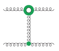
Refer to caption        Refer to caption

Figure 2: (a)(a) Tree five-gluon amplitude. The green blob along the gluon ladder represents the central-emission vertex. (b)(b) Regge trajectory in the one-loop four–gluon amplitude. The pierced blob represents the one-loop Regge trajectory.

The MRK rationale is that each gluon emitted along the ladder requires a factor of αS\alpha_{\scriptscriptstyle S} and after being integrated out in rapidity yields a factor of log⁡(s/|t|)\log(s/|t|), in such a way that each gluon emitted along the ladder contributes a factor of 𝒪⁡(αS​log⁡(s/|t|)){\cal O}(\alpha_{\scriptscriptstyle S}\log(s/|t|)). Five-gluon amplitudes in MRK allow one to compute the emission of a gluon along the gluon ladder. The factor associated to that gluon emission is called central-emission vertex, or Lipatov vertex Lipatov:1976zz. The central-emission vertex constitutes the kernel of the BFKL equation. Beyond five gluons, amplitudes in MRK assume an iterative structure, with a central-emission vertex for each gluon emitted along the ladder. Thus, the building blocks of the BFKL equation are the central-emission vertex at tree level, fig. 2(a)(a), and the Regge trajectory at one loop (7), fig. 2(b)(b). Finally, the impact factors (2) are not part of the gluon ladder, but sit at its ends, and when they are squared the constitute the jet impact factors and contribute to any jet cross section Mueller:1986ey; DelDuca:1993mn; Stirling:1994he; Andersen:2001kta; Andersen:2008gc; Andersen:2009nu; Andersen:2011hs which is computed through the BFKL equation.

1.2 The Regge limit at next-to-leading logarithmic accuracy

At next-to-leading-logarithmic (NLL) accuracy, keeping the s↔us\leftrightarrow u crossing symmetry (4) into account, the exchange of one Reggeised gluon of eq. (6) generalises to Fadin:1993wh

ℳg​g→g​g(−)​[8a]\displaystyle{\cal M}^{(-)[8_{a}]}_{gg\to gg} (10)
=\displaystyle= 12​[gS​(Fa′)a​c​Cg​(paνa,pa′νa′)]​st​[(sτ)α⁡(t)+(−sτ)α⁡(t)]​[gS​(Fb′)c​b​Cg​(pbνb,pb′νb′)],\displaystyle\frac{1}{2}\left[g_{\scriptscriptstyle S}(F^{a^{\prime}})_{ac}\,C^{g}(p_{a}^{\nu_{a}};p_{a^{\prime}}^{\nu_{a^{\prime}}})\right]{s\over t}\left[\left({s\over\tau}\right)^{\alpha(t)}+\left({-s\over\tau}\right)^{\alpha(t)}\right]\,\left[g_{\scriptscriptstyle S}(F^{b^{\prime}})_{cb}\,C^{g}(p_{b}^{\nu_{b}};p_{b^{\prime}}^{\nu_{b^{\prime}}})\right]\,,

where the colour and kinematic parts of the amplitude are each odd under s↔us\leftrightarrow u crossing. Further, by expanding the gluon Regge trajectory,

α⁡(t)=αS4​π​α(1)​(t)+(αS4​π)2​α(2)​(t)+𝒪⁡(αS3),\alpha(t)=\frac{\alpha_{\scriptscriptstyle S}}{4\pi}\alpha^{(1)}(t)+\left(\frac{\alpha_{\scriptscriptstyle S}}{4\pi}\right)^{2}\alpha^{(2)}(t)+{\cal O}(\alpha_{\scriptscriptstyle S}^{3})\,, (11)

with α(1)​(t)\alpha^{(1)}(t) given in eq. (7), and the helicity-conserving impact factor,

Cg​(pj∓,pj′±)=Cg⁡(0)​(pj∓,pj′±)​(1+αS4​π​C−⁣+g⁡(1)​(t,τ)+𝒪⁡(αS2)).C^{g}(p_{j}^{\mp};p_{j^{\prime}}^{\pm})=C^{g(0)}(p_{j}^{\mp};p_{j^{\prime}}^{\pm})\left(1+\frac{\alpha_{\scriptscriptstyle S}}{4\pi}C^{g(1)}_{-+}(t,\tau)+{\cal O}(\alpha_{\scriptscriptstyle S}^{2})\right)\,. (12)

with j=a,bj=a,b, see fig. 3, one can write the amplitude (10) as a double expansion in the strong coupling αS\alpha_{\scriptscriptstyle S} and in log⁡(s/τ)\log(s/\tau),

ℳg​g→g​g(−)​[8a]=ℳg​g→g​g(0)​(1+∑ℓ=1∞(αS4​π)ℓ​Mg​g→g​g(ℓ)​[8a]),{\cal M}^{(-)[8_{a}]}_{gg\to gg}={\cal M}^{(0)}_{gg\to gg}\left(1+\sum_{\ell=1}^{\infty}\left(\frac{\alpha_{\scriptscriptstyle S}}{4\pi}\right)^{\ell}M^{(\ell)[8_{a}]}_{gg\to gg}\right)\,, (13)

with

Mg​g→g​g(ℓ)​[8a]=∑i=0ℓMg​g→g​g(ℓ,i)​[8a]​logi⁡(sτ),M^{(\ell)[8_{a}]}_{gg\to gg}=\sum_{i=0}^{\ell}M^{(\ell,i)[8_{a}]}_{gg\to gg}\log^{i}\left(\frac{s}{\tau}\right)\,, (14)

where the Mg​g→g​g(ℓ,ℓ)​[8a]M^{(\ell,\ell)[8_{a}]}_{gg\to gg} coefficients have LL accuracy, the Mg​g→g​g(ℓ,ℓ−1)​[8a]M^{(\ell,\ell-1)[8_{a}]}_{gg\to gg} coefficients have NLL accuracy, and in general the Mg​g→g​g(ℓ,ℓ−k)​[8a]M^{(\ell,\ell-k)[8_{a}]}_{gg\to gg} coefficients have Nk​LL\mathrm{N^{k}LL} accuracy.

Refer to caption      Refer to caption

Figure 3: Impact factors in the one-loop four–gluon amplitude. The pierced blobs represent the one-loop impact factor Cg⁡(1)​(t)C^{g(1)}(t).

Beyond LL accuracy, in the gluon ladder the exchange of two or more Reggeised gluons may appear. Further, all the colour representations (5) exchanged in the tt channel may contribute. However, at NLL accuracy, the real part of the amplitude is entirely given by the antisymmetric octet 𝟖a{\bf 8}_{a} through eq. (10),

Re​[ℳg​g→g​g]N​L​L=Re⁡[ℳg​g→g​g(−)​[8a]],{\rm Re}\left[{\cal M}_{gg\to gg}\right]_{NLL}={\rm Re}\left[{\cal M}^{(-)[8_{a}]}_{gg\to gg}\right]\,, (15)

which, once eq. (10) is expanded at one and two loops reads,

Re​[ℳg​g→g​g(1)]N​L​L=α(1)​(t)​log⁡(sτ)+2​R​e​[Cg⁡(1)​(t,τ)],\displaystyle{\rm Re}\left[{\cal M}^{(1)}_{gg\to gg}\right]_{NLL}=\alpha^{(1)}(t)\log\left(\frac{s}{\tau}\right)+2{\rm Re}\big[C^{g(1)}(t,\tau)\big]\,,
Re​[ℳg​g→g​g(2)]N​L​L\displaystyle{\rm Re}\left[{\cal M}^{(2)}_{gg\to gg}\right]_{NLL} (16)
=12​(α(1)​(t))2​log2⁡(sτ)+(α(2)​(t)+2​R​e​[Cg⁡(1)​(t,τ)]​α(1)​(t))​log⁡(sτ).\displaystyle\qquad\qquad=\frac{1}{2}\left(\alpha^{(1)}(t)\right)^{2}\log^{2}\left(\frac{s}{\tau}\right)+\left(\alpha^{(2)}(t)+2{\rm Re}\big[C^{g(1)}(t,\tau)\big]\alpha^{(1)}(t)\right)\log\left(\frac{s}{\tau}\right)\,.

Beyond two loops, no more coefficients occur at NLL accuracy, i.e. the gluon-gluon scattering amplitude is uniquely determined by eq. (10), in terms of the two-loop Regge trajectory α(2)​(t)\alpha^{(2)}(t) Fadin:1995xg; Fadin:1996tb; Fadin:1995km; Blumlein:1998ib; DelDuca:2001gu and the one-loop impact factor C(1)C^{(1)} Fadin:1993wh; Fadin:1992zt; Fadin:1993qb; DelDuca:1998kx; Bern:1998sc. Accordingly, gluon Reggeisation is extended to NLL accuracy Fadin:2006bj; Fadin:2015zea. Further, because of eq. (10) factorisation still holds, so the amplitudes for quark-gluon or quark-quark scattering have the same form as eq. (10), up to replacing one or both colour and impact factors for gluons with the ones for quarks.

Likewise, the BFKL equation is extended to NLL accuracy Fadin:1998py; Ciafaloni:1998gs, which sums the terms of 𝒪⁡(αSn​logn−1⁡(s/τ)){\cal O}(\alpha_{\scriptscriptstyle S}^{n}\log^{n-1}(s/\tau)). At NLL accuracy, the kernel of the BFKL equation is given by the radiative corrections to the central-emission vertex, i.e. the emission of two gluons or of a quark-antiquark pair along the gluon ladder Fadin:1989kf; DelDuca:1995ki; Fadin:1996nw; DelDuca:1996nom; DelDuca:1996km, fig. 4(a)(a), and the one-loop corrections to the central-emission vertex Fadin:1993wh; Fadin:1994fj; Fadin:1996yv; DelDuca:1998cx; Bern:1998sc, fig. 4(b)(b). The infrared divergences of the radiative corrections to the central-emission vertex cancel the divergences of the two-loop Regge trajectory, fig. 4(c)(c). The emission of two gluons or of a quark-antiquark pair along the gluon ladder requires the adoption of a next-to-multi-Regge kinematics (NMRK), in which the gluons are strongly ordered in rapidity except for two gluons or for a quark-antiquark pair emitted along the gluon ladder. The NMRK rationale is that when the two gluons or the quark-antiquark pair are integrated out in rapidity, they yield a factor of 𝒪⁡(αS2​log⁡(s/τ)){\cal O}(\alpha_{\scriptscriptstyle S}^{2}\log(s/\tau)), thus contributing to NLL accuracy.

Refer to caption      Refer to caption      Refer to caption

Figure 4: (a)(a) Tree six–gluon amplitude. The oval blob represents the central-emission vertex – the emission of two gluons or of a quark-antiquark pair along the gluon ladder. (b)(b) One-loop five–gluon amplitude. The pierced blob represents the one-loop corrections to the central-emission vertex. (c)(c) Regge trajectory in the two-loop four–gluon amplitude. The double pierced oval represents the two-loop Regge trajectory.

Finally, in order to compute jet cross sections at NLL accuracy through the BFKL equation Colferai:2010wu; Ducloue:2013hia; Ducloue:2013bva, one needs to compute the jet impact factors at next-to-leading order (NLO) in αS\alpha_{\scriptscriptstyle S} Bartels:2001ge; Bartels:2002yj. To that effect, one needs the one-loop impact factor C(1)C^{(1)} and the impact factor for the emission of two gluons or of a quark-antiquark pair Fadin:1989kf; DelDuca:1995ki; Fadin:1996nw; DelDuca:1996nom; DelDuca:1996km, evaluated in NMRK, sec. C, in which the gluons are strongly ordered in rapidity except for two partons emitted at one end of the ladder.

At NLL accuracy, in addition to the imaginary part of the antisymmetric octet 𝟖a{\bf 8}_{a} in eq. (10)33 3 In order to avoid an imaginary part in the antisymmetric octet 𝟖a{\bf 8}_{a}, one can define the combination of logarithms Caron-Huot:2017fxr, L=12​(log⁡(sτ)+log⁡(uτ))=log⁡(sτ)−i​π2.L=\frac{1}{2}\left(\log\left(\frac{s}{\tau}\right)+\log\left(\frac{u}{\tau}\right)\right)=\log\left(\frac{s}{\tau}\right)-i\frac{\pi}{2}\,. (17) Using LL as the resummation parameter, one may identify odd(even)-signature states with the real (imaginary) part of the amplitude, and thus with the exchange of an odd (even) number of Reggeised gluons, which is a convenient bookkeping device to classify the various contributions to the tt-channel exchange. At the accuracy of our study, this is immaterial, and we will keep using log⁡(s/τ)\log(s/\tau) as the resummation parameter., all the colour representations which are even under s↔us\leftrightarrow u crossing (5), i.e. the singlet 𝟏{\bf 1}, the symmetric octet 𝟖s{\bf 8}_{s} and the 𝟐𝟕{\bf 27}, appear in the imaginary part of the gluon-gluon scattering amplitude, already in the non-logarithmic term of the one-loop amplitude Mg​g→g​g(1,0)M^{(1,0)}_{gg\to gg} DelDuca:1998kx. Just like the BFKL equation Kuraev:1976ge; Kuraev:1977fs; Balitsky:1978ic, which is described by the exchange of two Reggeised gluons in the tt channel and displays a cut in the ss channel, the imaginary part of the gluon-gluon amplitude features a cut and is described by the exchange of two Reggeised gluons Caron-Huot:2013fea; Caron-Huot:2017zfo, and just like the BFKL equation DelDuca:2013lma its finite parts can be expressed in terms of single-valued harmonic polylogarithms Caron-Huot:2020grv. The analyses of Refs. Caron-Huot:2017zfo; Caron-Huot:2020grv complete the study of gluon-gluon scattering amplitudes at NLL accuracy. We note that the imaginary part of the gluon-gluon amplitude at NLL accuracy can only contribute to a squared amplitude, and thus to a cross section, at next-to-next-to-leading-logarithmic (NNLL) accuracy.

1.3 Moving toward next-to-next-to-leading logarithmic accuracy

At NNLL accuracy, both the antisymmetric octet 𝟖a{\bf 8}_{a} (starting at two loops) and the 𝟏𝟎⊕𝟏𝟎¯{\bf 10}\oplus\overline{{\bf 10}} (starting at three loops) feature a cut in the ss channel, which is described by the exchange of three Reggeised gluons in the tt channel Fadin:2016wso; Caron-Huot:2017fxr; Fadin:2017nka. This is in addition to the exchange of one Reggeised gluon, which is still given by eq. (10). Thus, Regge pole factorisation, which is based on the exchange of one Reggeised gluon, does not hold any more DelDuca:2001gu. Accordingly, in the non-logarithmic term of the two-loop amplitude, Mg​g→g​g(2,0)M^{(2,0)}_{gg\to gg}, both the two-loop impact factor and the three-Reggeised-gluon exchange44 4 At NNLL accuracy, the three-Reggeised-gluon exchange is currently known up to four loops Falcioni:2020lvv. contribute.

However, in Mg​g→g​g(2,0)M^{(2,0)}_{gg\to gg}, the factorisation-violating term is a 1/ε21/\varepsilon^{2} pole, whose coefficient is subleading in NcN_{c} DelDuca:2001gu. Since it is an infrared pole, it can be analysed through infrared factorisation, which shows that, in addition to the usual diagonal terms of the colour octet exchange, also non-diagonal terms in the tt-channel colour basis contribute to the real part of Mg​g→g​g(2,0)M^{(2,0)}_{gg\to gg} Bret:2011xm; DelDuca:2011ae. Then one can disentangle the infrared poles of the two-loop impact factor (10) from the ones of factorisation-violating terms by identifying the impact factor with the diagonal terms and the factorisation-violating terms with the off-diagonal ones. Carrying this prescription on to the next loop order, one can predict how the infrared poles of the factorisation-violating term propagate into the single-logarithmic term of the three-loop amplitude Mg​g→g​g(3,1)M^{(3,1)}_{gg\to gg} DelDuca:2013ara; DelDuca:2014cya, and thus have a prescription to disentangle the infrared poles of the three-loop Regge trajectory, which should be given by the cusp anomalous dimension Korchemskaya:1996je, from the ones of the factorisation-violating terms. The disentanglement, which is based on such a prescription, has been confirmed by the explicit computation of the three-loop four-point function of 𝒩=4{\cal N}=4 SYM Henn:2016jdu. We stress, though, that the disentanglement above is valid only for the infrared poles through three loops. In order to predict factorisation-violating terms beyond three loops and including the finite terms, one must be able to compute the three Reggeised-gluon exchange Caron-Huot:2017fxr; Caron-Huot:2020grv.

The possibility of disentangling terms which are based on the exchange of one Reggeised gluon from factorisation-violating terms makes us hope that the BFKL equation, which is based on the exchange of one Reggeised gluon, could be extended to NNLL accuracy. Further, there are reasons, which are based on the integrability of amplitudes in MRK in the large NcN_{c} limit Lipatov:2009nt and on the colour structure of the corrections found through four loops in Ref. Falcioni:2020lvv, to believe that the Regge pole factorisation would be simpler in the large NcN_{c} limit. This warrants an analysis of the terms which would contribute to the BFKL equation at NNLL accuracy.

At NNLL accuracy, the kernel of the BFKL equation will be given by the emission of three partons along the gluon ladder DelDuca:1999iql; Antonov:2004hh; Duhr:2009uxa, evaluated in next-to-next-to-multi-Regge kinematics (NNMRK); by the one-loop corrections to the emission of two gluons or of a quark-antiquark pair along the gluon ladder, evaluated in NMRK; and by the two-loop corrections to the central-emission vertex. The last two contributions are yet to be determined. The infrared divergences of the contributions outlined above will cancel the divergences of the three-loop Regge trajectory, which is so far only known in a specific scheme Caron-Huot:2017fxr.

Finally, in order to compute jet cross sections at NNLL accuracy through the BFKL equation, one needs to compute the jet impact factors at next-to-next-to-leading order (NNLO) in αS\alpha_{\scriptscriptstyle S}. To that effect, one needs the tree impact factor for the emission of three partons at one end of the ladder DelDuca:1999iql, evaluated in NNMRK; the two-loop impact factor C(2)C^{(2)} DelDuca:2014cya, and the one-loop impact factor for the emission of two gluons or of a quark-antiquark pair, evaluated in NMRK. Further, one must include the square of the one-loop helicity-violating impact factor, which is recalled in eqs. (68) and (69).

1.4 Plan

Using the one-loop corrections to the five-gluon amplitudes Bern:1993mq and to the two-quark three-gluon amplitudes Bern:1994fz, in this paper we evaluate the one-loop impact factor for the emission of two gluons. This is the last ingredient which is necessary to evaluate the gluon-jet impact factor at NNLO accuracy in αS\alpha_{\scriptscriptstyle S}.

Sec. 2 is devoted to the computation of the one-loop impact factor for the emission of two gluons. Firstly, we recall the tree-level impact factor; then in sec. 2.1, we consider the one-loop five-gluon amplitude in NMRK, and apply the reggeisation ansatz to each colour-ordered amplitude (30); from that we extract in sec. 2.2 the one-loop impact factor for the emission of two gluons (41). These are the main results of the paper. Then, in order to verify that Regge factorisation holds at NLL accuracy in NMRK, we consider in sec. 2.3 the one-loop two-quark three-gluon amplitude in NMRK, and we extract again the one-loop impact factor for the emission of two gluons, finding agreement with the previous computation. Finally, in sec. 2.4 we compute the one-loop helicity-violating impact factor. In sec. 3, we draw our conclusions. Several appendices are given, which contain information about the kinematic approximations, and the one-loop five-point amplitudes in general kinematics and in NMRK.

2 The impact factor for the emission of two gluons

We consider the production of three gluons of momenta p1p_{1}, p2p_{2} and pb′p_{b^{\prime}} in the scattering of two gluons of momenta pap_{a} and pbp_{b}. We suppose that the outgoing gluons are in NMRK, sec. C, with rapidities and transverse momenta,

y1≃y2≫yb′;|p1⟂|≃|p2⟂|≃|pb′⟂|.y_{1}\simeq y_{2}\gg y_{b^{\prime}}\,;\qquad|p_{1\perp}|\simeq|p_{2\perp}|\simeq|p_{b^{\prime}\perp}|\,. (18)

In the NMRK region of eq. (18), the tree amplitude for the ga​gb→g1​g2​gb′g_{a}\,g_{b}\to g_{1}\,g_{2}\,g_{b^{\prime}} scattering is DelDuca:1996km

ℳg​g→g​g​g(0)|N​M​R​K=∑σ∈S2gS3​(Fdσ1​Fdσ2)a​c​(Fb′)c​b​m5​g(0)​(paνa,pσ1νσ1,pσ2νσ2,pb′νb′,pbνb)|N​M​R​K,\left.{\cal M}^{(0)}_{gg\to ggg}\right|_{NMRK}=\sum_{\sigma\in S_{2}}g_{\scriptscriptstyle S}^{3}\,(F^{d_{\sigma_{1}}}F^{d_{\sigma_{2}}})_{ac}(F^{b^{\prime}})_{cb}\,\left.m^{(0)}_{5g}(p_{a}^{\nu_{a}},p^{\nu_{\sigma_{1}}}_{\sigma_{1}},p^{\nu_{\sigma_{2}}}_{\sigma_{2}},p_{b^{\prime}}^{\nu_{b^{\prime}}},p_{b}^{\nu_{b}})\right|_{NMRK}\,, (19)

where the sum is over the permutations of the labels 1 and 2, and the colour-ordered amplitude is

m5​g(0)​(paνa,p1ν1,p2ν2,pb′νb′,pbνb)|N​M​R​K=Ag​g​(0)​(paνa,p1ν1,p2ν2)​st​Cg⁡(0)​(pbνb,pb′νb′),\left.m^{(0)}_{5g}(p_{a}^{\nu_{a}},p^{\nu_{1}}_{1},p^{\nu_{2}}_{2},p_{b^{\prime}}^{\nu_{b^{\prime}}},p_{b}^{\nu_{b}})\right|_{NMRK}=A^{gg(0)}(p_{a}^{\nu_{a}};p^{\nu_{1}}_{1},p^{\nu_{2}}_{2})\,\frac{s}{t}\,C^{g(0)}(p_{b}^{\nu_{b}};p_{b^{\prime}}^{\nu_{b^{\prime}}})\,, (20)

with s=pa+pbs=p_{a}+p_{b}, q=pb′+pbq=p_{b^{\prime}}+p_{b} and t≃−|q⟂|2t\simeq-|q_{\perp}|^{2}, fig. 5(a). Eq. (19) yields the five-gluon amplitude in terms of two colour-ordered amplitudes, again in agreement with the Bern-Carrasco-Johansson (BCJ) counting of (n−3)!(n-3)! independent colour-ordered amplitudes.

Refer to caption

Figure 5: Tree (a)(a) five–gluon amplitude for the ga​gb→g1​g2​gb′g_{a}\,g_{b}\to g_{1}\,g_{2}\,g_{b^{\prime}} scattering, and (b)(b) two-quark three–gluon amplitude for the ga​qb→g1​g2​qb′g_{a}\,q_{b}\to g_{1}\,g_{2}\,q_{b^{\prime}} scattering, in the NMRK of eq. (18). The oval blob represents the impact factor for the emission of two gluons.

In eq. (20), the impact factor Ag​g​(0)​(paνa,p1ν1,p2ν2)A^{gg(0)}(p_{a}^{\nu_{a}};p^{\nu_{1}}_{1},p^{\nu_{2}}_{2}) for g∗​g→g​gg^{*}\,g\rightarrow g\,g can be written as

Ag​g​(0)​(paνa,p1ν1,p2ν2)=Dg​g​(paνa,p1ν1,p2ν2)​Bν~​(p1,p2),A^{gg(0)}(p_{a}^{\nu_{a}};p^{\nu_{1}}_{1},p^{\nu_{2}}_{2})=D^{gg}(p_{a}^{\nu_{a}};p^{\nu_{1}}_{1},p^{\nu_{2}}_{2})B^{\tilde{\nu}}(p_{1},p_{2})\,, (21)

with

Dg​g​(pa−,p1+,p2+)\displaystyle D^{gg}(p_{a}^{-};p^{+}_{1},p^{+}_{2}) =\displaystyle= 1,\displaystyle 1\,,
Dg​g​(pa+,p1−,p2+)\displaystyle D^{gg}(p_{a}^{+};p^{-}_{1},p^{+}_{2}) =\displaystyle= x12,\displaystyle x_{1}^{2}\,, (22)
Dg​g​(pa+,p1+,p2−)\displaystyle D^{gg}(p_{a}^{+};p^{+}_{1},p^{-}_{2}) =\displaystyle= x22,\displaystyle x_{2}^{2}\,,

and

ν~=sign⁡(νa+ν1+ν2),\tilde{\nu}={\rm sign}(\nu_{a}+\nu_{1}+\nu_{2})\,, (23)

and55 5 Note that since (Fc)a​b=i​2​fa​c​b(F^{c})_{ab}=i\sqrt{2}f^{acb}, the coefficient (24) and the central-emission vertex (28) do not display the usual overall 2\sqrt{2} factor.

B+​(p1,p2)=p1⟂+p2⟂p1⟂​x1x2​1⟨12⟩,B^{+}(p_{1},p_{2})=\frac{p_{1\perp}+p_{2\perp}}{p_{1\perp}}\sqrt{\frac{x_{1}}{x_{2}}}\frac{1}{\langle 12\rangle}\,, (24)

and where the momentum fractions are

xi=pi+p1++p2+,i=1,2.x_{i}=\frac{p_{i}^{+}}{p_{1}^{+}+p_{2}^{+}}\,,\qquad i=1,2\,. (25)

The BB coefficient (24) displays a collinear divergence as p1⋅p2→0p_{1}\cdot p_{2}\to 0. The DD coefficients (22) are real, and so invariant under parity, while BB transforms under parity into its complex conjugate,

B−​(p1,p2)=[B+​(p1,p2)]∗.B^{-}(p_{1},p_{2})=[B^{+}(p_{1},p_{2})]^{\ast}\,. (26)

The impact factor Ag​g​(0)​(paνa,p2ν2,p1ν1)A^{gg(0)}(p_{a}^{\nu_{a}};p^{\nu_{2}}_{2},p^{\nu_{1}}_{1}) is obtained from eq. (21) by swapping the labels 1 and 2.

Since the five-gluon amplitude is a MHV amplitude, eq. (19) describes 2​(52)=202\binom{5}{2}=20 helicity configurations. However, at leading power in t/st/s, only 12 helicity configurations are leading. The impact factor (21) describes six helicity configurations, three out of which are given by eq. (22), and three more by parity conjugation. They are multiplied by the two given by the impact factor Cg⁡(0)​(pb∓,pb′±)C^{g(0)}(p_{b}^{\mp};p_{b^{\prime}}^{\pm}) (2). Then there are eight helicity configurations which are power suppressed in t/st/s. Three of them are associated to Cg⁡(0)​(pb−,pb′−)C^{g(0)}(p_{b}^{-};p_{b^{\prime}}^{-}), multiplied by the impact factor (21) with the helicity configurations (22), one is associated to Cg⁡(0)​(pb−,pb′−)C^{g(0)}(p_{b}^{-};p_{b^{\prime}}^{-}) multiplied by Ag​g​(0)​(pa+,p1+,p2+)A^{gg(0)}(p_{a}^{+};p^{+}_{1},p^{+}_{2}). The remaining four are obtained from the four above by parity conjugation.

In MRK, app. B, with p1+≫p2+p_{1}^{+}\gg p_{2}^{+}, the impact factor Ag​g​(0)​(paνa,p2ν2,p1ν1)A^{gg(0)}(p_{a}^{\nu_{a}};p^{\nu_{2}}_{2},p^{\nu_{1}}_{1}) is power suppressed in p2+/p1+p_{2}^{+}/p_{1}^{+} because of the FF coefficient (24), while Ag​g​(0)​(paνa,p1ν1,p2ν2)A^{gg(0)}(p_{a}^{\nu_{a}};p^{\nu_{1}}_{1},p^{\nu_{2}}_{2}) factorises as

limp1+≫p2+Ag​g​(0)​(paνa,p1ν1,p2ν2)=Cg⁡(0)​(paνa,p1ν1)​1t1​Vg⁡(0)​(q1,p2ν2),\lim_{p_{1}^{+}\gg p_{2}^{+}}A^{gg(0)}(p_{a}^{\nu_{a}};p^{\nu_{1}}_{1},p^{\nu_{2}}_{2})=C^{g(0)}(p_{a}^{\nu_{a}};p^{\nu_{1}}_{1})\,\frac{1}{t_{1}}\,V^{g(0)}(q_{1},p^{\nu_{2}}_{2})\,, (27)

where q1=−(pa+p1)q_{1}=-(p_{a}+p_{1}), q2=q1−p2q_{2}=q_{1}-p_{2}, t1=q12≃−q1⟂​q1⟂∗t_{1}=q_{1}^{2}\simeq-q_{1\perp}q_{1\perp}^{\ast}, and where Cg⁡(0)​(paνa,p1ν1)C^{g(0)}(p_{a}^{\nu_{a}};p^{\nu_{1}}_{1}) is given in eq. (2), while the tree central-emission vertex is

Vg⁡(0)​(q1,p2+)=q1⟂∗​q2⟂p2⟂.V^{g(0)}(q_{1},p^{+}_{2})=\frac{q_{1\perp}^{\ast}q_{2\perp}}{p_{2\perp}}\,. (28)

Accordingly, the five-gluon amplitude (19) takes the factorised form,

ℳg​g→g​g​g(0)|M​R​K\displaystyle\left.{\cal M}^{(0)}_{gg\to ggg}\right|_{MRK} =\displaystyle= s⁡[gS​(Fd1)a​c1​Cg⁡(0)​(paνa,p1ν1)]​1t1\displaystyle s\left[g_{\scriptscriptstyle S}(F^{d_{1}})_{ac_{1}}\,C^{g(0)}(p_{a}^{\nu_{a}};p_{1}^{\nu_{1}})\right]\,{1\over t_{1}}\, (29)
×\displaystyle\times [gS​(Fd2)c1​c2​Vg⁡(0)​(q1,p2ν2)]​1t2​[gS​(Fb′)c2​b​Cg⁡(0)​(pbνb,pb′νb′)].\displaystyle\left[g_{\scriptscriptstyle S}(F^{d_{2}})_{c_{1}c_{2}}\,V^{g(0)}(q_{1},p^{\nu_{2}}_{2})\right]\,{1\over t_{2}}\,\left[g_{\scriptscriptstyle S}(F^{b^{\prime}})_{c_{2}b}\,C^{g(0)}(p_{b}^{\nu_{b}};p_{b^{\prime}}^{\nu_{b^{\prime}}})\right]\,.

2.1 The one-loop five-gluon amplitude in the next-to-multi-Regge kinematics

In order to extend eq. (19) to loop level and to NLL accuracy, we note that the five-gluon amplitude in the NMRK region of eq. (18) retains the crossing symmetry under pb↔pb′p_{b}\leftrightarrow p_{b^{\prime}}. Using eq. (83), that is equivalent to a crossing symmetry of the colour-ordered amplitudes of eq. (19) under either s2​b↔s2​b′s_{2b}\leftrightarrow s_{2b^{\prime}} or s1​b↔s1​b′s_{1b}\leftrightarrow s_{1b^{\prime}}. Then, just like for the four-gluon amplitude (4), but in this case for each colour-ordered amplitude, we may consider states whose kinematic and colour coefficients have a definite signature under the suitable crossing, extend the reggeisation ansatz (10) to NMRK, and write

ℳg​g→g​g​g(−)​[8a]|N​M​R​K=∑σ∈S2gS3​(Fdσ1​Fdσ2)a​c​(Fb′)c​b​m5​g​(paνa,pσ1νσ1,pσ2νσ2,pb′νb′,pbνb)|N​M​R​K,\left.{\cal M}^{(-)[8_{a}]}_{gg\to ggg}\right|_{NMRK}=\sum_{\sigma\in S_{2}}g_{\scriptscriptstyle S}^{3}\,(F^{d_{\sigma_{1}}}F^{d_{\sigma_{2}}})_{ac}(F^{b^{\prime}})_{cb}\,\left.m_{5g}(p_{a}^{\nu_{a}},p^{\nu_{\sigma_{1}}}_{\sigma_{1}},p^{\nu_{\sigma_{2}}}_{\sigma_{2}},p_{b^{\prime}}^{\nu_{b^{\prime}}},p_{b}^{\nu_{b}})\right|_{NMRK}\,, (30)

where, as in eq. (19), the sum is over the permutations of the labels 1 and 2, and

m5​g​(paνa,p1ν1,p2ν2,pb′νb′,pbνb)|N​M​R​K\displaystyle\left.m_{5g}(p_{a}^{\nu_{a}},p^{\nu_{1}}_{1},p^{\nu_{2}}_{2},p_{b^{\prime}}^{\nu_{b^{\prime}}},p_{b}^{\nu_{b}})\right|_{NMRK} (31)
=\displaystyle= 12​st​Ag​g​(paνa,p1ν1,p2ν2)​[(s2​b′τ)α⁡(t)+(−s2​b′τ)α⁡(t)]​Cg​(pbνb,pb′νb′),\displaystyle\frac{1}{2}{s\over t}A^{gg}(p_{a}^{\nu_{a}};p^{\nu_{1}}_{1},p^{\nu_{2}}_{2})\left[\left({s_{2b^{\prime}}\over\tau}\right)^{\alpha(t)}+\left({-s_{2b^{\prime}}\over\tau}\right)^{\alpha(t)}\right]C^{g}(p_{b}^{\nu_{b}};p_{b^{\prime}}^{\nu_{b^{\prime}}})\,,

where α⁡(t)\alpha(t) is given by eq. (11), Cg​(pbνb,pb′νb′)C^{g}(p_{b}^{\nu_{b}};p_{b^{\prime}}^{\nu_{b^{\prime}}}) by eq. (12), and

Ag​g​(paνa,p1ν1,p2ν2)=Ag​g​(0)​(paνa,p1ν1,p2ν2)​(1+αS4​π​Aν~g​g​(1)​(p1,p2,τ)+𝒪⁡(αS2)),A^{gg}(p_{a}^{\nu_{a}};p^{\nu_{1}}_{1},p^{\nu_{2}}_{2})=A^{gg(0)}(p_{a}^{\nu_{a}};p^{\nu_{1}}_{1},p^{\nu_{2}}_{2})\left(1+\frac{\alpha_{\scriptscriptstyle S}}{4\pi}A^{gg(1)}_{\tilde{\nu}}(p_{1},p_{2},\tau)+{\cal O}(\alpha_{\scriptscriptstyle S}^{2})\right)\,, (32)

with ν~\tilde{\nu} in eq. (23). Just like in eq. (13), one can write the colour-ordered amplitude (31) as a double expansion in the strong coupling αS\alpha_{\scriptscriptstyle S} and in log⁡(s2​b′/τ)\log(s_{2b^{\prime}}/\tau),

m5​g|N​M​R​K=m5​g(0)​(1+∑ℓ=1∞(αS4​π)ℓ​m5​g(ℓ)),\left.m_{5g}\right|_{NMRK}=m^{(0)}_{5g}\left(1+\sum_{\ell=1}^{\infty}\left(\frac{\alpha_{\scriptscriptstyle S}}{4\pi}\right)^{\ell}m^{(\ell)}_{5g}\right)\,, (33)

with m5​g(0)m^{(0)}_{5g} as in eq. (20) where a N​M​R​KNMRK subscript is understood, and where

m5​g(ℓ)=∑i=0ℓlogi⁡(s2​b′τ)​m5​g(ℓ,i),m^{(\ell)}_{5g}=\sum_{i=0}^{\ell}\log^{i}\left(\frac{s_{2b^{\prime}}}{\tau}\right)m^{(\ell,i)}_{5g}\,, (34)

where the m5​g(ℓ,ℓ)m^{(\ell,\ell)}_{5g} coefficients have LL accuracy, the m5​g(ℓ,ℓ−1)m^{(\ell,\ell-1)}_{5g} coefficients have NLL accuracy, etc.

If at NLL accuracy only the antisymmetric octet 𝟖a{\bf 8}_{a} is exchanged in the tt channel, and if within 𝟖a{\bf 8}_{a} three reggeised-gluon exchanges are missing, we expect that, just like for eq. (10), the real part of the five-gluon amplitude in the NMRK region of eq. (18) be entirely given by eq. (30),

Re​[ℳg​g→g​g​g]N​M​R​KN​L​L=Re​[ℳg​g→g​g​g(−)​[8a]]N​M​R​K,{\rm Re}\left[{\cal M}_{gg\to ggg}\right]^{NLL}_{NMRK}={\rm Re}\left[{\cal M}^{(-)[8_{a}]}_{gg\to ggg}\right]_{NMRK}\,, (35)

where the left-hand side of eq. (35), once expanded at one loop, yields

Re[ℳg​g→g​g​g(1)]N​M​R​KN​L​L=gS3αS4​π∑σ∈S2(Fdσ1Fdσ2Fb′)a​bRe[m5:1]N​M​R​K,{\rm Re}\left[{\cal M}^{(1)}_{gg\to ggg}\right]_{NMRK}^{NLL}=g_{\scriptscriptstyle S}^{3}\,\frac{\alpha_{\scriptscriptstyle S}}{4\pi}\,\sum_{\sigma\in S_{2}}(F^{d_{\sigma_{1}}}F^{d_{\sigma_{2}}}F^{b^{\prime}})_{ab}\,{\rm Re}\left[m_{5:1}\right]_{NMRK}\,, (36)

where the colour-ordered amplitude m5:1m_{5:1} will be provided in app. E and app. F, where the dependence on the momenta to be permuted is understood, and where, using eqs. (33) and (35), we write

Re[m5:1]N​M​R​K=m5​g(0)Re[m5​g(1)]N​M​R​K,{\rm Re}\left[m_{5:1}\right]_{NMRK}=m^{(0)}_{5g}\,{\rm Re}\left[m^{(1)}_{5g}\right]_{NMRK}\,, (37)

with

Re​[m5​g(1)]N​M​R​K=α(1)​(t)​log⁡(s2​b′τ)+Re⁡[Ag​g​(1)​(p1,p2,τ)]+Re⁡[Cg⁡(1)​(t,τ)],{\rm Re}\left[m^{(1)}_{5g}\right]_{NMRK}=\alpha^{(1)}(t)\log\left(\frac{s_{2b^{\prime}}}{\tau}\right)+{\rm Re}\big[A^{gg(1)}(p_{1},p_{2},\tau)\big]+{\rm Re}\big[C^{g(1)}(t,\tau)\big]\,, (38)

which is displayed diagrammatically in fig. 6.

Refer to caption

Figure 6: Factorisation of the one-loop five-gluon amplitude in NMRK. The three diagrams represent the three terms in eq. (37). The pierced blobs represent (a)(a) the one-loop Regge trajectory; and the one-loop corrections to the impact factor for the emission of (b)(b) two gluons and (c)(c) one gluon.

The one-loop impact factors Cp⁡(1)C^{p(1)}, with p=g,qp=g,q, are process and infrared-scheme dependent. They were computed in conventional dimensional regularization (CDR)/’t-Hooft-Veltman (HV) schemes in Refs. Fadin:1992zt; Fadin:1993wh; Fadin:1993qb; DelDuca:1998kx; Bern:1998sc, and in the dimensional reduction (DR)/ four dimensional helicity (FDH) schemes in Refs. Bern:1998sc; DelDuca:1998kx. Through 𝒪⁡(ε0){\cal O}(\varepsilon^{0}), the real part of the MS¯\overline{\rm MS}-renormalised one-loop gluon impact factor can be written as DelDuca:1998kx; DelDuca:2017pmn

Re⁡[C−⁣+g⁡(1)​(t,τ)]\displaystyle{\rm Re}\big[C^{g(1)}_{-+}(t,\tau)\big] =\displaystyle= κΓ{(μ2−t)ε[−γK(1)ϵ2Nc+4​γg(1)ϵ+β02​ε+Ncεlog(τ−t)\displaystyle\kappa_{\Gamma}\left\{\left({\mu^{2}\over-t}\right)^{\varepsilon}\left[-\frac{\gamma_{K}^{(1)}}{\epsilon^{2}}N_{c}+\frac{4\gamma_{g}^{(1)}}{\epsilon}+\frac{\beta_{0}}{2\varepsilon}+\frac{N_{c}}{\varepsilon}\log\left(\frac{\tau}{-t}\right)\right.\right. (39)
−(329+δR6−π22)Nc+59Nf]−β02​ε}\displaystyle\left.\left.\qquad\qquad\quad-\left(\frac{32}{9}+\frac{\delta_{R}}{6}-\frac{\pi^{2}}{2}\right)N_{c}+\frac{5}{9}N_{f}\right]-\frac{\beta_{0}}{2\varepsilon}\right\}
=\displaystyle= κΓ[(μ2−t)ϵ[(−2ϵ2−116​ε+1εlog(τ−t)−329−δR6+π22)Nc\displaystyle\kappa_{\Gamma}\left[\left(\frac{\mu^{2}}{-t}\right)^{\epsilon}\left[\left(-\frac{2}{\epsilon^{2}}-\frac{11}{6\varepsilon}+\frac{1}{\varepsilon}\log\left(\frac{\tau}{-t}\right)-\frac{32}{9}-\frac{\delta_{R}}{6}+\frac{\pi^{2}}{2}\right)N_{c}\right.\right.
+(13​ε+59)Nf]−β02​ϵ],\displaystyle\left.\left.\qquad\qquad\quad+\left(\frac{1}{3\varepsilon}+\frac{5}{9}\right)N_{f}\right]-\frac{\beta_{0}}{2\epsilon}\right]\,,

with NfN_{f} the number of light quark flavours, and where we have used the regularisation parameter, δR=1\delta_{R}=1 in CDR/HV schemes, δR=0\delta_{R}=0 in the DR/FDH schemes Catani:1996pk. In eq. (39), the last term is the MS¯\overline{\rm MS} ultraviolet counterterm, and the infrared ε\varepsilon poles are accounted for by the cusp anomalous dimension and by the gluon collinear anomalous dimension DelDuca:2014cya, with γK(1)\gamma_{K}^{(1)} the one-loop coefficient of the cusp anomalous dimension (86), γg(1)\gamma_{g}^{(1)} the one-loop coefficient of the gluon collinear anomalous dimension (88), and β0\beta_{0} the one-loop coefficient of the beta function (89).

In order to compute Ag​g​(1)A^{gg(1)}, we use the colour decomposition of the one-loop five-gluon amplitude DelDuca:1999rs,

ℳ5​g(1)\displaystyle{\cal M}^{(1)}_{5g} =\displaystyle= gS5∑σ∈S4/ℛ[Tr (Fdσ1⋯Fdσ5)m5:1[1](σ1,…,σ5)\displaystyle g_{\scriptscriptstyle S}^{5}\sum_{\sigma\in S_{4}/{\cal R}}\left[\mbox{Tr\,}(F^{d_{\sigma_{1}}}\cdots F^{d_{\sigma_{5}}})m_{5:1}^{[1]}(\sigma_{1},\ldots,\sigma_{5})\right. (40)
+2NfTr (Tdσ1⋯Tdσ5)m5:1[1/2](σ1,…,σ5)],\displaystyle\left.\qquad+2N_{f}\mbox{Tr\,}(T^{d_{\sigma_{1}}}\cdots T^{d_{\sigma_{5}}})m_{5:1}^{[1/2]}(\sigma_{1},\ldots,\sigma_{5})\right]\,,

where S4≡S5/ℤ5S_{4}\equiv S_{5}/\mathbb{Z}_{5} is the group of the non-cyclic permutations, and ℛ{\cal R} is the reflection: ℛ⁡(1,…,5)=(5,…,1){\cal R}(1,\ldots,5)=(5,\ldots,1). The superscript [j][j] denotes the spin of the particle circulating in the loop. Eq. (40) contains 12 independent colour-ordered amplitudes of type m5:1[1]m_{5:1}^{[1]} and 12 of type m5:1[1/2]m_{5:1}^{[1/2]}. They have been computed in Ref. Bern:1993mq, and are recorded in app. E in the notation of Ref. DelDuca:1998cx.

We evaluate the colour-ordered amplitudes m5:1[1]m_{5:1}^{[1]} and m5:1[1/2]m_{5:1}^{[1/2]}, app. E, in the NMRK region of eq. (18) and app. C. The leading colour-ordered amplitudes are found to be the same as at tree level (19), such that at one loop we can write the five-gluon colour-ordered amplitude as in eq. (36), where m5:1m_{5:1} is given by eqs. (98) and (102). Then the one-loop five-gluon amplitude is factorised as in eqs. (30)-(37).

2.2 One-loop impact factor for the emission of two gluons

Using eqs. (7), (37) and (39), we obtain from eq. (102) the real part of the MS¯\overline{\rm MS}-renormalised one-loop impact factor for the emission of two gluons,

1κΓ​Re​[A+g​g​(1)​(p1,p2,τ)]\displaystyle\frac{1}{\kappa_{\Gamma}}{\rm Re}\big[A^{gg(1)}_{+}(p_{1},p_{2},\tau)\big] (41)
=\displaystyle= Nc{−1ϵ2[2(μ2|p1⟂|2)ϵ+(μ2|p2⟂|2)ϵ]\displaystyle N_{c}\left\{-\frac{1}{\epsilon^{2}}\left[2\left(\frac{\mu^{2}}{|p_{1\perp}|^{2}}\right)^{\epsilon}+\left(\frac{\mu^{2}}{|p_{2\perp}|^{2}}\right)^{\epsilon}\right]\right.
+1ϵ​[2​(μ2|p1⟂|2)ϵ​log⁡(s12|p1⟂|​|p2⟂|)+(μ2−t)ϵ​log⁡(τ|p2⟂|2)]\displaystyle\qquad+\frac{1}{\epsilon}\left[2\left(\frac{\mu^{2}}{|p_{1\perp}|^{2}}\right)^{\epsilon}\log\left(\frac{s_{12}}{|p_{1\perp}|\>|p_{2\perp}|}\right)+\left(\frac{\mu^{2}}{-t}\right)^{\epsilon}\log\left(\frac{\tau}{|p_{2\perp}|^{2}}\right)\right]
−1ϵ​(μ2−t​|p2⟂|2|p1⟂|2​(p2+p1+​s12|p2⟂|2)12)ϵ​log⁡(x1​x2​s12|p2⟂|2)\displaystyle\qquad-\frac{1}{\epsilon}\left(\frac{\mu^{2}}{-t}\frac{|p_{2\perp}|^{2}}{|p_{1\perp}|^{2}}\left(\frac{p_{2}^{+}}{p_{1}^{+}}\frac{s_{12}}{|p_{2\perp}|^{2}}\right)^{\frac{1}{2}}\right)^{\epsilon}\log\left(\frac{x_{1}x_{2}s_{12}}{|p_{2\perp}|^{2}}\right)
−12log2(|p1⟂|2−t)−12log(x1)log(x1x2(−ts12)3−t|p2⟂|2)−329−δR6+56π2}\displaystyle\left.\qquad-\frac{1}{2}\log^{2}\left(\frac{|p_{1\perp}|^{2}}{-t}\right)-\frac{1}{2}\log\left(x_{1}\right)\log\left(x_{1}x_{2}\left(\frac{-t}{s_{12}}\right)^{3}\frac{-t}{|p_{2\perp}|^{2}}\right)-\frac{32}{9}-\frac{\delta_{R}}{6}+\frac{5}{6}\pi^{2}\right\}
−\displaystyle- β02​ϵ​(x1​μ2|p1⟂|2)ϵ+59​Nf+β02​(|p1⟂|2x1−t+2​q⟂∗​p1⟂)​L0​(|p1⟂|2−x1​t)t\displaystyle\frac{\beta_{0}}{2\epsilon}\left(\frac{x_{1}\mu^{2}}{|p_{1\perp}|^{2}}\right)^{\epsilon}+\frac{5}{9}N_{f}+\frac{\beta_{0}}{2}\left(\frac{|p_{1\perp}|^{2}}{x_{1}}-t+2q_{\perp}^{*}p_{1\perp}\right)\frac{L_{0}\left(\frac{|p_{1\perp}|^{2}}{-x_{1}t}\right)}{t}
+\displaystyle+ NC−Nf3{p2+p1+[|p1⟂|2q⟂∗2p2⟂2−2|p1⟂|2|p2⟂|2p1⟂q⟂∗+p2+p1+|p1⟂|4p2⟂q⟂∗]\displaystyle\frac{N_{C}-N_{f}}{3}\left\{\frac{p_{2}^{+}}{p_{1}^{+}}\left[|p_{1\perp}|^{2}\>{q_{\perp}^{*}}^{2}\>p_{2\perp}^{2}-2\>|p_{1\perp}|^{2}\>|p_{2\perp}|^{2}p_{1\perp}q_{\perp}^{*}+\frac{p_{2}^{+}}{p_{1}^{+}}|p_{1\perp}|^{4}\,p_{2\perp}q_{\perp}^{*}\right]\right.
−|p2⟂|2[2|p1⟂|2(−t)+(2|p2⟂|2−|p1⟂|2+t)p1⟂q⟂∗]}L2​(|p1⟂|2−x1​t)t3\displaystyle\qquad\qquad-|p_{2\perp}|^{2}\left[2\>|p_{1\perp}|^{2}(-t)+\left(2\,|p_{2\perp}|^{2}-|p_{1\perp}|^{2}+t\right)p_{1\perp}q_{\perp}^{*}\right]\bigg\}\frac{L_{2}\left(\frac{|p_{1\perp}|^{2}}{-x_{1}t}\right)}{t^{3}}
+\displaystyle+ NC−Nf6​[x2​p2⟂​q⟂∗−t+2​x1​x2​q⟂∗2​p1⟂2−t​|p1⟂|2−x1​|p2⟂|2​p1⟂​q⟂∗−t​|p1⟂|2]−β0ϵ+O⁡(ϵ),\displaystyle\frac{N_{C}-N_{f}}{6}\left[\frac{x_{2}p_{2\perp}q_{\perp}^{*}}{-t}+\frac{2x_{1}x_{2}{q_{\perp}^{*}}^{2}p_{1\perp}^{2}}{-t\,|p_{1\perp}|^{2}}-\frac{x_{1}|p_{2\perp}|^{2}p_{1\perp}q_{\perp}^{*}}{-t\,|p_{1\perp}|^{2}}\right]-\frac{\beta_{0}}{\epsilon}+O(\epsilon)\,,

with q⟂=−(p1⟂+p2⟂)q_{\perp}=-(p_{1\perp}+p_{2\perp}), where the last term is the MS¯\overline{\rm MS} ultraviolet counterterm, and where it is understood that in order to obtain the real part we must use eq. (103). The impact factor Ag​g​(1)​(paνa,p2ν2,p1ν1)A^{gg(1)}(p_{a}^{\nu_{a}};p^{\nu_{2}}_{2},p^{\nu_{1}}_{1}) for the second colour ordering of eq. (30) is obtained by exchanging the labels 1 and 2 in eq. (41).

In MRK, app. B, with p1+≫p2+p_{1}^{+}\gg p_{2}^{+}, the impact factor Ag​g​(paνa,p2ν2,p1ν1)A^{gg}(p_{a}^{\nu_{a}};p^{\nu_{2}}_{2},p^{\nu_{1}}_{1}) is power suppressed in p2+/p1+p_{2}^{+}/p_{1}^{+}, then we just need to consider the first colour ordering in eq. (30), for which the one-loop impact factor (41) factorises as

limp1+≫p2+Re⁡[Ag​g​(1)​(p1,p2,τ)]=α(1)​(t1)​log⁡(s12τ)+Re⁡[Cg⁡(1)​(t1,τ)]+Re⁡[Vg⁡(1)​(q1,p2,τ)],\lim_{p_{1}^{+}\gg p_{2}^{+}}{\rm Re}\big[A^{gg(1)}(p_{1},p_{2},\tau)\big]=\alpha^{(1)}(t_{1})\log\left(\frac{s_{12}}{\tau}\right)+{\rm Re}\big[C^{g(1)}(t_{1},\tau)\big]+{\rm Re}\big[V^{g(1)}(q_{1},p_{2},\tau)\big]\,, (42)

with q1=−(pa+p1)q_{1}=-(p_{a}+p_{1}), t1=q12≃−q1⟂​q1⟂∗t_{1}=q_{1}^{2}\simeq-q_{1\perp}q_{1\perp}^{\ast} and q=q2=q1−p2q=q_{2}=q_{1}-p_{2}, and where the one-loop corrections to the MS¯\overline{\rm MS}-renormalised central-emission vertex (28) are given by

Vg​(q1,p2)=Vg⁡(0)​(q1,p2)​(1+αS4​π​Vg⁡(1)​(q1,p2,τ)+𝒪⁡(αS2)),V^{g}(q_{1},p_{2})=V^{g(0)}(q_{1},p_{2})\left(1+\frac{\alpha_{\scriptscriptstyle S}}{4\pi}V^{g(1)}(q_{1},p_{2},\tau)+{\cal O}(\alpha_{\scriptscriptstyle S}^{2})\right)\,, (43)

with DelDuca:1998cx

1κΓ​Re⁡[Vg⁡(1)​(q1,p2,τ)]\displaystyle\frac{1}{\kappa_{\Gamma}}\hbox to0.0pt{$\displaystyle{\rm Re}\big[V^{g(1)}(q_{1},p_{2},\tau)\big]$\hss} (44)
=\displaystyle= Nc​{−1ϵ2​(μ2|p2⟂|2)ϵ+1ϵ​[(μ2−t1)ϵ+(μ2−t2)ϵ]​log⁡(τ|p2⟂|2)−12​log2⁡(t1t2)+π23}\displaystyle N_{c}\left\{-{1\over\epsilon^{2}}\,\left({\mu^{2}\over|p_{2\perp}|^{2}}\right)^{\epsilon}+{1\over\epsilon}\,\left[\left({\mu^{2}\over-t_{1}}\right)^{\epsilon}+\left({\mu^{2}\over-t_{2}}\right)^{\epsilon}\right]\log\left({\tau\over|p_{2\perp}|^{2}}\right)-{1\over 2}\log^{2}\left({t_{1}\over t_{2}}\right)+{\pi^{2}\over 3}\right\}
−\displaystyle- β02​(t1+t2+2​q1⟂​q2⟂∗)​L0​(t1/t2)t2\displaystyle{\beta_{0}\over 2}\left(t_{1}+t_{2}+2q_{1\perp}q_{2\perp}^{\ast}\right){L_{0}(t_{1}/t_{2})\over t_{2}}
+\displaystyle+ Nc−Nf3​|p2⟂|2​[−[2​t1​t2+(t1+t2+2​|p2⟂|2)​q1⟂​q2⟂∗]​L2​(t1/t2)t23−q1⟂​q2⟂∗2​t1​t2]−β02​ϵ\displaystyle{N_{c}-N_{f}\over 3}\,|p_{2\perp}|^{2}\left[-[2t_{1}t_{2}+(t_{1}+t_{2}+2|p_{2\perp}|^{2})q_{1\perp}q_{2\perp}^{\ast}]{L_{2}(t_{1}/t_{2})\over t_{2}^{3}}-{q_{1\perp}q_{2\perp}^{\ast}\over 2\,t_{1}\,t_{2}}\right]-{\beta_{0}\over 2\epsilon}
+\displaystyle+ O⁡(ϵ),\displaystyle O(\epsilon)\,,

with t=t2=q22t=t_{2}=q_{2}^{2}, where the last term is the MS¯\overline{\rm MS} ultraviolet counterterm, and where it is understood that in order to obtain the real part we must use

2​Re​(q1⟂​q2⟂∗)=−(t1+t2+|p2⟂|2).2{\rm Re}(q_{1\perp}q_{2\perp}^{\ast})=-(t_{1}+t_{2}+|p_{2\perp}|^{2})\,. (45)

2.3 One-loop two-quark three-gluon amplitude in NMRK

Regge factorisation at tree level implies that in the NMRK region of eq. (18), we can write the two-quark three-gluon tree amplitude for the ga​qb→g1​g2​qb′g_{a}\,q_{b}\to g_{1}\,g_{2}\,q_{b^{\prime}} scattering, fig. 5(b), as DelDuca:1996km; DelDuca:1999iql

ℳg​q→g​g​q(0)|N​M​R​K=∑σ∈S2gS3​(Fdσ1​Fdσ2)a​c​(Tc)b′​b¯​m2​q​3​g(0)​(paνa,pσ1νσ1,pσ2νσ2,pb′νb′,pbνb)|N​M​R​K,\left.{\cal M}^{(0)}_{gq\to ggq}\right|_{NMRK}=\sum_{\sigma\in S_{2}}g_{\scriptscriptstyle S}^{3}\,(F^{d_{\sigma_{1}}}F^{d_{\sigma_{2}}})_{ac}(T^{c})_{b^{\prime}\bar{b}}\,\left.m^{(0)}_{2q3g}(p_{a}^{\nu_{a}},p^{\nu_{\sigma_{1}}}_{\sigma_{1}},p^{\nu_{\sigma_{2}}}_{\sigma_{2}},p_{b^{\prime}}^{\nu_{b^{\prime}}},p_{b}^{\nu_{b}})\right|_{NMRK}\,, (46)

where the sum is over the permutations of the labels 1 and 2, and the colour-ordered amplitude is

m2​q​3​g(0)​(paνa,p1ν1,p2ν2,pb′νb′,pbνb)|N​M​R​K=Ag​g​(0)​(paνa,p1ν1,p2ν2)​st​Cq⁡(0)​(pbνb,pb′νb′),\left.m^{(0)}_{2q3g}(p_{a}^{\nu_{a}},p^{\nu_{1}}_{1},p^{\nu_{2}}_{2},p_{b^{\prime}}^{\nu_{b^{\prime}}},p_{b}^{\nu_{b}})\right|_{NMRK}=A^{gg(0)}(p_{a}^{\nu_{a}};p^{\nu_{1}}_{1},p^{\nu_{2}}_{2})\,\frac{s}{t}\,C^{q(0)}(p_{b}^{\nu_{b}};p_{b^{\prime}}^{\nu_{b^{\prime}}})\,, (47)

where Ag​g​(0)A^{gg(0)} is given by eq. (21), and the quark impact factor is66 6 Since helicities are for all outgoing momenta, an incoming right-handed quark is labelled in eq. (48) and the right-hand side of eq. (46) as a left-handed antiquark, so e.g. the amplitude gR​(−pa)​qR​(−pb)→gR​(p1)​gR​(p2)​qR​(pb′)g_{R}(-p_{a})q_{R}(-p_{b})\to g_{R}(p_{1})g_{R}(p_{2})q_{R}(p_{b^{\prime}}) becomes ℳ⁡(ag−,1g+,2g+,b′q+,bq¯−){\cal M}(a^{-}_{g},1^{+}_{g},2^{+}_{g},{b^{\prime}}^{+}_{q},b^{-}_{\bar{q}}).

Cq⁡(0)​(pb−,pb′+)=i​pb′⟂∗pb′⟂,C^{q(0)}(p_{b}^{-};p_{b^{\prime}}^{+})=i\sqrt{p_{b^{\prime}\perp}^{*}\over p_{b^{\prime}\perp}}\,, (48)

which under parity becomes DelDuca:1999iql

[Cq⁡(0)​(pb−ν,pb′ν)]∗=S​Cq⁡(0)​(pbν,pb′−ν)withS=−sign⁡(q¯0​q0).[C^{q(0)}(p_{b}^{-\nu};p_{b^{\prime}}^{\nu})]^{\ast}=SC^{q(0)}(p_{b}^{\nu};p_{b^{\prime}}^{-\nu})\qquad{\rm with}\quad S=-{\rm sign}({\bar{q}}^{0}q^{0})\,. (49)

If Regge factorisation holds at NLL accuracy, then we can write the two-quark three-gluon amplitude in the NMRK region of eq. (18) as

ℳg​q→g​g​q(−)​[8a]|N​M​R​K=∑σ∈S2gS3​(Fdσ1​Fdσ2)a​c​(Tc)b′​b¯​m2​q​3​g​(paνa,pσ1νσ1,pσ2νσ2,pb′νb′,pbνb)|N​M​R​K,\left.{\cal M}^{(-)[8_{a}]}_{gq\to ggq}\right|_{NMRK}=\sum_{\sigma\in S_{2}}g_{\scriptscriptstyle S}^{3}\,(F^{d_{\sigma_{1}}}F^{d_{\sigma_{2}}})_{ac}(T^{c})_{b^{\prime}\bar{b}}\,\left.m_{2q3g}(p_{a}^{\nu_{a}},p^{\nu_{\sigma_{1}}}_{\sigma_{1}},p^{\nu_{\sigma_{2}}}_{\sigma_{2}},p_{b^{\prime}}^{\nu_{b^{\prime}}},p_{b}^{\nu_{b}})\right|_{NMRK}\,, (50)

with the colour-ordered amplitude,

m2​q​3​g​(paνa,p1ν1,p2ν2,pb′νb′,pbνb)|N​M​R​K\displaystyle\left.m_{2q3g}(p_{a}^{\nu_{a}},p^{\nu_{1}}_{1},p^{\nu_{2}}_{2},p_{b^{\prime}}^{\nu_{b^{\prime}}},p_{b}^{\nu_{b}})\right|_{NMRK} (51)
=\displaystyle= 12​st​Ag​g​(paνa,p1ν1,p2ν2)​[(s2​b′τ)α⁡(t)+(−s2​b′τ)α⁡(t)]​Cq​(pbνb,pb′νb′),\displaystyle\frac{1}{2}{s\over t}A^{gg}(p_{a}^{\nu_{a}};p^{\nu_{1}}_{1},p^{\nu_{2}}_{2})\left[\left({s_{2b^{\prime}}\over\tau}\right)^{\alpha(t)}+\left({-s_{2b^{\prime}}\over\tau}\right)^{\alpha(t)}\right]C^{q}(p_{b}^{\nu_{b}};p_{b^{\prime}}^{\nu_{b^{\prime}}})\,,

where Ag​g​(paνa,p1ν1,p2ν2)A^{gg}(p_{a}^{\nu_{a}};p^{\nu_{1}}_{1},p^{\nu_{2}}_{2}) is given by eq. (32), and Cq​(pbνb,pb′νb′)C^{q}(p_{b}^{\nu_{b}};p_{b^{\prime}}^{\nu_{b^{\prime}}}) is given by the quark analog of eq. (12). We can then write the colour-ordered amplitude (51) as a double expansion in the strong coupling αS\alpha_{\scriptscriptstyle S} and in log⁡(s2​b′/τ)\log(s_{2b^{\prime}}/\tau), and repeat the steps of eq. (33) through eq. (37). Once expanded at one loop, the real part of eq. (51) becomes

Re​[m2​q​3​g(1)]N​M​R​K=α(1)​(t)​log⁡(sσ2​b′τ)+Re⁡[Ag​g​(1)​(pσ1,pσ2,τ)]+Re⁡[Cq⁡(1)​(t,τ)],{\rm Re}\left[m^{(1)}_{2q3g}\right]_{NMRK}=\alpha^{(1)}(t)\log\left(\frac{s_{\sigma_{2}b^{\prime}}}{\tau}\right)+{\rm Re}\big[A^{gg(1)}(p_{\sigma_{1}},p_{\sigma_{2}},\tau)\big]+{\rm Re}\big[C^{q(1)}(t,\tau)\big]\,, (52)

with Ag​g​(1)A^{gg(1)} as in eq. (41), and where, through 𝒪⁡(ε0){\cal O}(\varepsilon^{0}), the MS¯\overline{\rm MS}-renormalised one-loop quark impact factor Cq⁡(1)​(t)C^{q(1)}(t) can be written as DelDuca:1998kx; DelDuca:2017pmn

Re⁡[C−⁣+q⁡(1)​(t,τ)]\displaystyle{\rm Re}\big[C^{q(1)}_{-+}(t,\tau)\big] =\displaystyle= κΓ{(μ2−t)ϵ[−γK(1)ϵ2CF+4εγq(1)+β02​ε+Ncεlog(τ−t)\displaystyle\kappa_{\Gamma}\left\{\left({\mu^{2}\over-t}\right)^{\epsilon}\left[-\frac{\gamma_{K}^{(1)}}{\epsilon^{2}}C_{F}+\frac{4}{\varepsilon}\gamma_{q}^{(1)}+\frac{\beta_{0}}{2\varepsilon}+\frac{N_{c}}{\varepsilon}\log\left(\frac{\tau}{-t}\right)\right.\right. (53)
+(1918−δR3+π22)Nc−59Nf+(72+δR2)1Nc]−β02​ε}\displaystyle\left.\left.\qquad\qquad+\left({19\over 18}-{\delta_{R}\over 3}+{\pi^{2}\over 2}\right)N_{c}-\frac{5}{9}N_{f}+\left({7\over 2}+{\delta_{R}\over 2}\right){1\over N_{c}}\right]-\frac{\beta_{0}}{2\varepsilon}\right\}
=\displaystyle= κΓ{(μ2−t)ϵ[(−1ϵ2+13​ϵ+1εlog(τ−t)+1918−δR3+π22)Nc\displaystyle\kappa_{\Gamma}\left\{\left({\mu^{2}\over-t}\right)^{\epsilon}\left[\left(-{1\over\epsilon^{2}}+{1\over 3\epsilon}+\frac{1}{\varepsilon}\log\left(\frac{\tau}{-t}\right)+{19\over 18}-{\delta_{R}\over 3}+{\pi^{2}\over 2}\right)N_{c}\right.\right.
−(13​ϵ+59)Nf+(1ϵ2+32​ϵ+72+δR2)1Nc]−β02​ϵ},\displaystyle\qquad\left.\left.-\left({1\over 3\epsilon}+{5\over 9}\right)N_{f}+\left({1\over\epsilon^{2}}+{3\over 2\epsilon}+{7\over 2}+{\delta_{R}\over 2}\right){1\over N_{c}}\right]-{\beta_{0}\over 2\epsilon}\right\}\,,

with γq(1)\gamma_{q}^{(1)} the one-loop coefficient of the quark collinear anomalous dimension (88).

In order to verify that the one-loop two-quark three-gluon amplitude in NMRK takes the factorised form given by eq. (52), we use the colour decomposition of the one-loop two-quark three-gluon amplitude DelDuca:1999rs,

M2​q​3​g1−l​o​o​p​(1q¯,2q,3,4,5)\displaystyle M_{2q3g}^{1-loop}(1_{\bar{q}},2_{q},3,4,5) (54)
=\displaystyle= gS5[∑p=25∑σ∈S3(Tc2Tdσ3…TdσpTc1)i2i¯1(Fdσp+1…Fdσ5)c1​c2\displaystyle g_{\scriptscriptstyle S}^{5}\left[\sum_{p=2}^{5}\sum_{\sigma\in S_{3}}\left(T^{c_{2}}T^{d_{\sigma_{3}}}\ldots T^{d_{\sigma_{p}}}T^{c_{1}}\right)_{i_{2}}^{\,\,\bar{i}_{1}}\left(F^{d_{\sigma_{p+1}}}\ldots F^{d_{\sigma_{5}}}\right)_{c_{1}c_{2}}\right.
×A5R,[1]​(1q¯,σp+1,…,σ5,2q,σ3,…,σp)\displaystyle\qquad\times A_{5}^{R,[1]}(1_{\bar{q}},\sigma_{p+1},\ldots,\sigma_{5},2_{q},\sigma_{3},\ldots,\sigma_{p})
+NfNc∑j=14∑σ∈S3/S5;jGr5;jq¯​q(σ3,σ4,σ5)A5;j[1/2](1q¯,2q,σ3,σ4,σ5)],\displaystyle\quad+\left.\frac{N_{f}}{N_{c}}\sum_{j=1}^{4}\sum_{\sigma\in S_{3}/S_{5;j}}Gr_{5;j}^{\bar{q}q}(\sigma_{3},\sigma_{4},\sigma_{5})A_{5;j}^{[1/2]}(1_{\bar{q}},2_{q},\sigma_{3},\sigma_{4},\sigma_{5})\right]\,,

where the colour structures G​r5;jq¯​qGr_{5;j}^{\bar{q}q} are defined by

G​r5;1q¯​q​(3,4,5)\displaystyle Gr_{5;1}^{\bar{q}q}(3,4,5) =\displaystyle= Nc​(Td3​Td4​Td5)i2i¯1,\displaystyle N_{c}\left(T^{d_{3}}T^{d_{4}}T^{d_{5}}\right)_{i_{2}}^{\,\,\bar{i}_{1}}\,,
G​r5;2q¯​q​(3,4,5)\displaystyle Gr_{5;2}^{\bar{q}q}(3;4,5) =\displaystyle= 0,\displaystyle 0\,,
G​r5;3q¯​q​(3,4,5)\displaystyle Gr_{5;3}^{\bar{q}q}(3,4;5) =\displaystyle= Tr ​(Td3​Td4)​(Td5)i2i¯1,\displaystyle\mbox{Tr\,}\left(T^{d_{3}}T^{d_{4}}\right)\left(T^{d_{5}}\right)_{i_{2}}^{\,\,\bar{i}_{1}}\,,
G​r5;4q¯​q​(3,4,5)\displaystyle Gr_{5;4}^{\bar{q}q}(3,4;5) =\displaystyle= Tr ​(Td3​Td4​Td5)​δi2i¯1,\displaystyle\mbox{Tr\,}\left(T^{d_{3}}T^{d_{4}}T^{d_{5}}\right)\delta_{i_{2}}^{\,\,\bar{i}_{1}}\,, (55)

and S5;j=ℤj−1S_{5;j}=\mathbb{Z}_{j-1} is the subgroup of S3S_{3} that leaves G​r5;jq¯​qGr_{5;j}^{\bar{q}q} invariant, and

A5;1[1/2]​(1q¯,2q,3,4,5)\displaystyle A_{5;1}^{[1/2]}(1_{\bar{q}},2_{q},3,4,5) =\displaystyle= A5L,[1/2]​(1q¯,2q,3,4,5),\displaystyle A_{5}^{L,[1/2]}(1_{\bar{q}},2_{q},3,4,5)\,,
A5;3[1/2]​(1q¯,2q,3,4,5)\displaystyle A_{5;3}^{[1/2]}(1_{\bar{q}},2_{q};3,4;5) =\displaystyle= −∑σ∈{4,3}⊔⊔{1,2,5}A5;1[1/2](σ(1q¯,2q,3,4,5)),\displaystyle-\sum_{\sigma\in\{4,3\}\sqcup\mathchoice{\mkern-7.0mu}{\mkern-7.0mu}{\mkern-3.2mu}{\mkern-3.8mu}\sqcup\{1,2,5\}}A_{5;1}^{[1/2]}\left(\sigma(1_{\bar{q}},2_{q},3,4,5)\right)\,,
A5;4[1/2]​(1q¯,2q,3,4,5)\displaystyle A_{5;4}^{[1/2]}(1_{\bar{q}},2_{q};3,4;5) =\displaystyle= ∑σ∈{5,4,3}⊔⊔{1,2}A5;1[1/2]​(σ⁡(1q¯,2q,3,4,5)),\displaystyle\sum_{\sigma\in\{5,4,3\}\sqcup\mathchoice{\mkern-7.0mu}{\mkern-7.0mu}{\mkern-3.2mu}{\mkern-3.8mu}\sqcup\{1,2\}}A_{5;1}^{[1/2]}\left(\sigma(1_{\bar{q}},2_{q},3,4,5)\right)\,, (56)

where the shuffle product {α}⊔⊔{β}\{\alpha\}\sqcup\mathchoice{\mkern-7.0mu}{\mkern-7.0mu}{\mkern-3.2mu}{\mkern-3.8mu}\sqcup\{\beta\} yields the permutations which preserve the orderings of the elements in {α}\{\alpha\} and in {β}\{\beta\} while allowing for all possible orderings of the elements of {α}\{\alpha\} with respect to {β}\{\beta\}. In eq. (56), we did not list the j=2j=2 case, since the corresponding colour structure is missing in eq. (55). Further, we spell out the first sum of eq. (54),

∑p=25∑σ∈S3(Tc2​Tdσ3​…​Tdσp​Tc1)i2i¯1​(Fdσp+1​…​Fdσ5)c1​c2\displaystyle\sum_{p=2}^{5}\sum_{\sigma\in S_{3}}\left(T^{c_{2}}T^{d_{\sigma_{3}}}\ldots T^{d_{\sigma_{p}}}T^{c_{1}}\right)_{i_{2}}^{\,\,\bar{i}_{1}}\left(F^{d_{\sigma_{p+1}}}\ldots F^{d_{\sigma_{5}}}\right)_{c_{1}c_{2}} (57)
×A5R,[1]​(1q¯,σp+1,…,σ5,2q,σ3,…,σp)\displaystyle\qquad\times A_{5}^{R,[1]}(1_{\bar{q}},\sigma_{p+1},\ldots,\sigma_{5},2_{q},\sigma_{3},\ldots,\sigma_{p})
=\displaystyle= ∑σ∈S3[(Tc2Tc1)i2i¯1(Fdσ3Fdσ4Fdσ5)c1​c2A5R,[1](1q¯,σ3,σ4,σ5,2q)\displaystyle\sum_{\sigma\in S_{3}}\left[\left(T^{c_{2}}T^{c_{1}}\right)_{i_{2}}^{\,\,\bar{i}_{1}}\left(F^{d_{\sigma_{3}}}F^{d_{\sigma_{4}}}F^{d_{\sigma_{5}}}\right)_{c_{1}c_{2}}A_{5}^{R,[1]}(1_{\bar{q}},\sigma_{3},\sigma_{4},\sigma_{5},2_{q})\right.
+(Tc2​Tdσ3​Tc1)i2i¯1​(Fdσ4​Fdσ5)c1​c2​A5R,[1]​(1q¯,σ4,σ5,2q,σ3)\displaystyle\qquad+\left(T^{c_{2}}T^{d_{\sigma_{3}}}T^{c_{1}}\right)_{i_{2}}^{\,\,\bar{i}_{1}}\left(F^{d_{\sigma_{4}}}F^{d_{\sigma_{5}}}\right)_{c_{1}c_{2}}A_{5}^{R,[1]}(1_{\bar{q}},\sigma_{4},\sigma_{5},2_{q},\sigma_{3})
+(Tc2​Tdσ3​Tdσ4​Tc1)i2i¯1​(Fdσ5)c1​c2​A5R,[1]​(1q¯,σ5,2q,σ3,σ4)\displaystyle\qquad+\left(T^{c_{2}}T^{d_{\sigma_{3}}}T^{d_{\sigma_{4}}}T^{c_{1}}\right)_{i_{2}}^{\,\,\bar{i}_{1}}\left(F^{d_{\sigma_{5}}}\right)_{c_{1}c_{2}}A_{5}^{R,[1]}(1_{\bar{q}},\sigma_{5},2_{q},\sigma_{3},\sigma_{4})
+(Tc2Tdσ3Tdσ4Tdσ5Tc1)i2i¯1δc1​c2A5R,[1](1q¯,2q,σ3,σ4,σ5)].\displaystyle\left.\qquad+\left(T^{c_{2}}T^{d_{\sigma_{3}}}T^{d_{\sigma_{4}}}T^{d_{\sigma_{5}}}T^{c_{1}}\right)_{i_{2}}^{\,\,\bar{i}_{1}}\delta_{c_{1}c_{2}}A_{5}^{R,[1]}(1_{\bar{q}},2_{q},\sigma_{3},\sigma_{4},\sigma_{5})\right]\,.

Finally, the reflection identity,

AnR,[1]​(1q¯,3,…,2q,…,n−1,n)=(−1)n​AnL,[1]​(1q¯,n,n−1,…,2q,…,3).A_{n}^{R,[1]}(1_{\bar{q}},3,\ldots,2_{q},\ldots,n-1,n)=(-1)^{n}A_{n}^{L,[1]}(1_{\bar{q}},n,n-1,\ldots,2_{q},\ldots,3)\,. (58)

relates the left and right primitive amplitudes.

The primitive amplitudes A5L,[1]​(1q¯,2q,3,4,5)A_{5}^{L,[1]}(1_{\bar{q}},2_{q},3,4,5) and A5L,[1/2]​(1q¯,2q,3,4,5)A_{5}^{L,[1/2]}(1_{\bar{q}},2_{q},3,4,5), which are necessary to assemble the one-loop two-quark three-gluon amplitude (54), have been provided by Ref. Bern:1994fz in the DR/FDH schemes. We have evaluated them in the NMRK region of eq. (18) and app. C. In NMRK, the leading contributions are given by the terms with p=2p=2, p=5p=5 and j=1j=1 in eq. (54), i.e. by the first and the last term on the right-hand side of eq. (57) and by the first term of eqs. (55) and (56).

2.3.1 The p=2p=2 term

The knowledge of the primitive amplitudes A5L,[1]​(1q¯,2q,3,4,5)A_{5}^{L,[1]}(1_{\bar{q}},2_{q},3,4,5) Bern:1994fz, and the reflection identity (58) allow us to compute the primitive amplitudes A5R,[1]A_{5}^{R,[1]}, which, in the notation of the ga​qb→g1​g2​qb′g_{a}\,q_{b}\to g_{1}\,g_{2}\,q_{b^{\prime}} scattering, are A5R,[1]​(bq¯,σa,σ1,σ2,b′q)A_{5}^{R,[1]}(b_{\bar{q}},\sigma_{a},\sigma_{1},\sigma_{2},{b^{\prime}}_{q}). Computing the primitive amplitudes A5R,[1]A_{5}^{R,[1]} in the NMRK of eq. (18) for different colour orderings, we find that they are related by,

A5R,[1]​(bq¯,a,1,2,b′q)\displaystyle A_{5}^{R,[1]}(b_{\bar{q}},a,1,2,{b^{\prime}}_{q}) =\displaystyle= A5R,[1]​(bq¯,2,1,a,b′q)=−λ1​m2​q​3​g(0)​(pa,p1,p2,pb′,pb),\displaystyle A_{5}^{R,[1]}(b_{\bar{q}},2,1,a,{b^{\prime}}_{q})=-\lambda_{1}m_{2q3g}^{(0)}(p_{a},p_{1},p_{2},p_{b^{\prime}},p_{b})\,,
A5R,[1]​(bq¯,a,2,1,b′q)\displaystyle A_{5}^{R,[1]}(b_{\bar{q}},a,2,1,{b^{\prime}}_{q}) =\displaystyle= A5R,[1]​(bq¯,1,2,a,b′q)=−λ2​m2​q​3​g(0)​(pa,p2,p1,pb′,pb),\displaystyle A_{5}^{R,[1]}(b_{\bar{q}},1,2,a,{b^{\prime}}_{q})=-\lambda_{2}m_{2q3g}^{(0)}(p_{a},p_{2},p_{1},p_{b^{\prime}},p_{b})\,,
A5R,[1]​(bq¯,1,a,2,b′q)\displaystyle A_{5}^{R,[1]}(b_{\bar{q}},1,a,2,{b^{\prime}}_{q}) =\displaystyle= A5R,[1]​(bq¯,2,a,1,b′q)\displaystyle A_{5}^{R,[1]}(b_{\bar{q}},2,a,1,{b^{\prime}}_{q}) (59)
=\displaystyle= λ1​m2​q​3​g(0)​(pa,p1,p2,pb′,pb)+λ2​m2​q​3​g(0)​(pa,p2,p1,pb′,pb),\displaystyle\lambda_{1}m_{2q3g}^{(0)}(p_{a},p_{1},p_{2},p_{b^{\prime}},p_{b})+\lambda_{2}m_{2q3g}^{(0)}(p_{a},p_{2},p_{1},p_{b^{\prime}},p_{b})\,,

with λ1,λ2\lambda_{1},\lambda_{2} in eqs. (105) and (106), and m2​q​3​g(0)​(pa,p2,p1,pb′,pb)m_{2q3g}^{(0)}(p_{a},p_{2},p_{1},p_{b^{\prime}},p_{b}) the tree colour-ordered amplitude (47), where a N​M​R​KNMRK subscript is understood. Using eq. (59), the colour coefficient of the p=2p=2 term of eq. (54), i.e. of the first term on the right-hand side of eq. (57), simplifies and factors an NcN_{c} term out. It can be written as

∑σ∈S3(Tc2​Tc1)b′b¯​(Fdσa​Fdσ1​Fdσ2)c1​c2​A5R,[1]​(bq¯,σa,σ1,σ2,b′q)\displaystyle\sum_{\sigma\in S_{3}}\left(T^{c_{2}}T^{c_{1}}\right)_{b^{\prime}}^{\,\,\bar{b}}\left(F^{d_{\sigma_{a}}}F^{d_{\sigma_{1}}}F^{d_{\sigma_{2}}}\right)_{c_{1}c_{2}}A_{5}^{R,[1]}(b_{\bar{q}},\sigma_{a},\sigma_{1},\sigma_{2},{b^{\prime}}_{q})
⟹N​M​R​KNc​∑σ∈S2(Fdσ1​Fdσ2)a​c​(Tc)b′b¯​λσ1​m2​q​3​g(0)​(pa,pσ1,pσ2,pb′,pb).\displaystyle\stackrel{{\scriptstyle\scriptscriptstyle NMRK}}{{\Longrightarrow}}N_{c}\sum_{\sigma\in S_{2}}(F^{d_{\sigma_{1}}}F^{d_{\sigma_{2}}})_{ac}\,(T^{c})_{b^{\prime}}^{\bar{b}}\lambda_{\sigma_{1}}m_{2q3g}^{(0)}(p_{a},p_{\sigma_{1}},p_{\sigma_{2}},p_{b^{\prime}},p_{b})\,. (60)

Thus, the p=2p=2 term provides the leading NcN_{c} terms of the one-loop two-quark three-gluon amplitude in NMRK.

2.3.2 The p=5p=5 term

For the p=5p=5 term, one can use the relation Bern:1994fz,

A5R,[1]​(bq¯,b′q,σa,σ1,σ2)\displaystyle A_{5}^{R,[1]}(b_{\bar{q}},{b^{\prime}}_{q},\sigma_{a},\sigma_{1},\sigma_{2}) (61)
=\displaystyle= A5S​U​S​Y​(bq¯,b′q,σa,σ1,σ2)−A5L,[1]​(bq¯,b′q,σa,σ1,σ2)−A5L,[1/2]​(bq¯,b′q,σa,σ1,σ2),\displaystyle A_{5}^{SUSY}(b_{\bar{q}},{b^{\prime}}_{q},\sigma_{a},\sigma_{1},\sigma_{2})-A_{5}^{L,[1]}(b_{\bar{q}},{b^{\prime}}_{q},\sigma_{a},\sigma_{1},\sigma_{2})-A_{5}^{L,[1/2]}(b_{\bar{q}},{b^{\prime}}_{q},\sigma_{a},\sigma_{1},\sigma_{2})\,,

where the primitive amplitudes on the right-hand side are all provided in Ref. Bern:1994fz. Computing the primitive amplitudes A5R,[1]A_{5}^{R,[1]} in the NMRK of eq. (18) for different colour orderings, we find that they are related by

A5R,[1]​(bq¯,bq′,a,1,2)\displaystyle A_{5}^{R,[1]}(b_{\bar{q}},b^{\prime}_{q},a,1,2) =\displaystyle= A5R,[1]​(bq¯,bq′,2,1,a)=Φ​m2​q​3​g(0)​(pa,p1,p2,pb,pb′),\displaystyle A_{5}^{R,[1]}(b_{\bar{q}},b^{\prime}_{q},2,1,a)=\Phi\,m_{2q3g}^{(0)}(p_{a},p_{1},p_{2},p_{b},p_{b^{\prime}})\,,
A5R,[1]​(bq¯,bq′,a,2,1)\displaystyle A_{5}^{R,[1]}(b_{\bar{q}},b^{\prime}_{q},a,2,1) =\displaystyle= A5R,[1]​(bq¯,bq′,1,2,a)=Φ​m2​q​3​g(0)​(pa,p2,p1,pb,pb′),\displaystyle A_{5}^{R,[1]}(b_{\bar{q}},b^{\prime}_{q},1,2,a)=\Phi\,m_{2q3g}^{(0)}(p_{a},p_{2},p_{1},p_{b},p_{b^{\prime}})\,,
A5R,[1]​(bq¯,bq′,1,a,2)\displaystyle A_{5}^{R,[1]}(b_{\bar{q}},b^{\prime}_{q},1,a,2) =\displaystyle= A5R,[1]​(bq¯,bq′,2,a,1)\displaystyle A_{5}^{R,[1]}(b_{\bar{q}},b^{\prime}_{q},2,a,1) (62)
=\displaystyle= −Φ⁡[m2​q​3​g(0)​(pa,p1,p2,pb,pb′)+m2​q​3​g(0)​(pa,p2,p1,pb,pb′)],\displaystyle-\Phi\left[m_{2q3g}^{(0)}(p_{a},p_{1},p_{2},p_{b},p_{b^{\prime}})+m_{2q3g}^{(0)}(p_{a},p_{2},p_{1},p_{b},p_{b^{\prime}})\right],

where m2​q​3​g(0)​(pa,p1,p2,pb,pb′)=−m2​q​3​g(0)​(pa,p1,p2,pb′,pb)m_{2q3g}^{(0)}(p_{a},p_{1},p_{2},p_{b},p_{b^{\prime}})=-m_{2q3g}^{(0)}(p_{a},p_{1},p_{2},p_{b^{\prime}},p_{b}), and with

Φ=κΓ​(μ2−t)ϵ​(1ϵ2+32​ϵ+72).\Phi=\kappa_{\Gamma}\left(\frac{\mu^{2}}{-t}\right)^{\epsilon}\left(\frac{1}{\epsilon^{2}}+\frac{3}{2\epsilon}+\frac{7}{2}\right)\,. (63)

Using eq. (62), the colour coefficient of the p=5p=5 term of eq. (54), i.e. of the fourth term on the right-hand side of eq. (57), simplifies and factors a 1/Nc1/N_{c} term out. It can be written as

∑σ∈S3δc1​c2​(Tc2​Tdσa​Tdσ1​Tdσ2​Tc1)b′b¯​A5R,[1]​(bq¯,bq′,σa,σ1,σ2)\displaystyle\sum_{\sigma\in S_{3}}\delta_{c_{1}c_{2}}\left(T^{c_{2}}T^{d_{\sigma_{a}}}T^{d_{\sigma_{1}}}T^{d_{\sigma_{2}}}T^{c_{1}}\right)_{b^{\prime}}^{\,\,\bar{b}}A_{5}^{R,[1]}(b_{\bar{q}},b^{\prime}_{q},\sigma_{a},\sigma_{1},\sigma_{2})
⟹N​M​R​K1Nc​Φ​∑σ∈S2(Fdσ1​Fdσ2)a​c​(Tc)b′b¯​λσ1​m2​q​3​g(0)​(pa,pσ1,pσ2,pb,pb′).\displaystyle\stackrel{{\scriptstyle\scriptscriptstyle NMRK}}{{\Longrightarrow}}\frac{1}{N_{c}}\Phi\sum_{\sigma\in S_{2}}(F^{d_{\sigma_{1}}}F^{d_{\sigma_{2}}})_{ac}\,(T^{c})_{b^{\prime}}^{\bar{b}}\lambda_{\sigma_{1}}m_{2q3g}^{(0)}(p_{a},p_{\sigma_{1}},p_{\sigma_{2}},p_{b},p_{b^{\prime}})\,. (64)

Thus, the p=5p=5 term provides the 1/Nc1/N_{c} terms of the one-loop two-quark three-gluon amplitude in NMRK.

2.3.3 The j=1j=1 term

For the j=1j=1 term, we use the first term of eqs. (55) and (56). Computing the primitive amplitudes A5;1[1/2]A^{[1/2]}_{5;1} in the NMRK of eq. (18) for different colour orderings, we find that they are related by,

A5;1[1/2]​(bq¯,bq′,a,1,2)\displaystyle A^{[1/2]}_{5;1}(b_{\bar{q}},b^{\prime}_{q},a,1,2) =\displaystyle= A5;1[1/2]​(bq¯,bq′,2,1,a)=χ1​m2​q​3​g(0)​(pa,p1,p2,pb,pb′),\displaystyle A^{[1/2]}_{5;1}(b_{\bar{q}},b^{\prime}_{q},2,1,a)=\chi_{1}\,m_{2q3g}^{(0)}(p_{a},p_{1},p_{2},p_{b},p_{b^{\prime}})\,,
A5;1[1/2]​(bq¯,bq′,a,2,1)\displaystyle A^{[1/2]}_{5;1}(b_{\bar{q}},b^{\prime}_{q},a,2,1) =\displaystyle= A5;1[1/2]​(bq¯,bq′,1,2,a)=χ2​m2​q​3​g(0)​(pa,p2,p1,pb,pb′),\displaystyle A^{[1/2]}_{5;1}(b_{\bar{q}},b^{\prime}_{q},1,2,a)=\chi_{2}\,m_{2q3g}^{(0)}(p_{a},p_{2},p_{1},p_{b},p_{b^{\prime}})\,,
A5;1[1/2]​(bq¯,bq′,1,a,2)\displaystyle A^{[1/2]}_{5;1}(b_{\bar{q}},b^{\prime}_{q},1,a,2) =\displaystyle= A5;1[1/2]​(bq¯,bq′,2,a,1)\displaystyle A^{[1/2]}_{5;1}(b_{\bar{q}},b^{\prime}_{q},2,a,1) (65)
=\displaystyle= −χ1​m2​q​3​g(0)​(pa,p1,p2,pb,pb′)−χ2​m2​q​3​g(0)​(pa,p2,p1,pb,pb′),\displaystyle-\chi_{1}m_{2q3g}^{(0)}(p_{a},p_{1},p_{2},p_{b},p_{b^{\prime}})-\chi_{2}m_{2q3g}^{(0)}(p_{a},p_{2},p_{1},p_{b},p_{b^{\prime}})\,,

with χ1,χ2\chi_{1},\chi_{2} in eqs. (107) and (108). Using eq. (65), the colour coefficient of the j=1j=1 term of eq. (54) simplifies and can be written as

Nf​∑σ∈S3(Tdσa​Tdσ1​Tdσ2)b′b¯​A5;1[1/2]​(bq¯,bq′,σa,σ1,σ2)\displaystyle N_{f}\sum_{\sigma\in S_{3}}\left(T^{d_{\sigma_{a}}}T^{d_{\sigma_{1}}}T^{d_{\sigma_{2}}}\right)_{b^{\prime}}^{\,\,\bar{b}}A^{[1/2]}_{5;1}(b_{\bar{q}},b^{\prime}_{q},\sigma_{a},\sigma_{1},\sigma_{2})
⟹N​M​R​KNf​∑σ∈S2(Fdσ1​Fdσ2)a​c​(Tc)b′b¯​χσ1​m2​q​3​g(0)​(pa,pσ1,pσ2,pb,pb′).\displaystyle\stackrel{{\scriptstyle\scriptscriptstyle NMRK}}{{\Longrightarrow}}N_{f}\sum_{\sigma\in S_{2}}(F^{d_{\sigma_{1}}}F^{d_{\sigma_{2}}})_{ac}\,(T^{c})_{b^{\prime}}^{\bar{b}}\chi_{\sigma_{1}}m_{2q3g}^{(0)}(p_{a},p_{\sigma_{1}},p_{\sigma_{2}},p_{b},p_{b^{\prime}})\,. (66)

Thus, the j=1j=1 term provides the NfN_{f} terms of the one-loop two-quark three-gluon amplitude in NMRK.

2.3.4 Regge factorisation

Combining eqs. (60) and (64) and (66), we obtain the one-loop two-quark three-gluon amplitude in the NMRK region of eq. (18),

Re​[ℳg​q→g​g​q(1)]N​M​R​K\displaystyle{\rm Re}\left[{\cal M}^{(1)}_{gq\to ggq}\right]_{NMRK} (67)
=\displaystyle= ∑σ∈S2(Fdσ1​Fdσ2)a​c​(Tc)b′b¯​(Nc​λσ1+Nf​χσ1+ΦNc)​m2​q​3​g(0)​(pa,pσ1,pσ2,pb′,pb).\displaystyle\sum_{\sigma\in S_{2}}(F^{d_{\sigma_{1}}}F^{d_{\sigma_{2}}})_{ac}\,(T^{c})_{b^{\prime}}^{\bar{b}}\left(N_{c}\lambda_{\sigma_{1}}+N_{f}\chi_{\sigma_{1}}+\frac{\Phi}{N_{c}}\right)m_{2q3g}^{(0)}(p_{a},p_{\sigma_{1}},p_{\sigma_{2}},p_{b^{\prime}},p_{b})\,.

Then we use eq. (52), with the one-loop Regge trajectory (7) and the one-loop quark impact factor (53), which in particular subtracts out all the 1/Nc1/N_{c} terms, and we obtain the one-loop impact factor for the emission of two gluons Ag​g​(1)A^{gg(1)}, which is in agreement with eq. (41), thus verifying that Regge factorisation holds at NLL accuracy in NMRK.

2.4 Helicity-violating contributions

The conservation of helicity along the ss-channel direction in Minkowski space, that we mentioned in the Introduction, is an approximate feature of the Regge limit of tree four-gluon amplitudes, since the helicity-flip impact factor Cg⁡(0)​(p+,p′⁣+)C^{g(0)}(p^{+};p^{\prime+}) exists, but is power suppressed in t/st/s. At one loop, the four-gluon amplitude m4(1)​(−,+,+,+)m_{4}^{(1)}(-,+,+,+) is not vanishing, so the helicity-flip impact factor Cg⁡(1)​(p+,p′⁣+)C^{g(1)}(p^{+};p^{\prime+}) is not power suppressed in t/st/s Fadin:1993wh; Fadin:1992zt; DelDuca:1998kx. In fact, we can write

Cg​(pj+,pj′+)=Cg⁡(0)​(pj−,pj′+)​(αS4​π​C+⁣+g⁡(1)​(q⟂)+𝒪⁡(αS2)),C^{g}(p_{j}^{+};p_{j^{\prime}}^{+})=C^{g(0)}(p_{j}^{-};p_{j^{\prime}}^{+})\left(\frac{\alpha_{\scriptscriptstyle S}}{4\pi}C^{g(1)}_{++}(q_{\perp})+{\cal O}(\alpha_{\scriptscriptstyle S}^{2})\right)\,, (68)

with j=a,bj=a,b and q⟂=pb′⟂=−pa′⟂q_{\perp}=p_{b^{\prime}\perp}=-p_{a^{\prime}\perp}, and

C+⁣+g⁡(1)​(q⟂)=−Nc−Nf3​q⟂∗q⟂.C^{g(1)}_{++}(q_{\perp})=-\frac{N_{c}-N_{f}}{3}\,\frac{q_{\perp}^{\ast}}{q_{\perp}}\,. (69)

Because the tree four-gluon amplitude m4(0)​(−,+,+,+)m_{4}^{(0)}(-,+,+,+) vanishes, the one loop four-gluon amplitude m4(1)​(−,+,+,+)m_{4}^{(1)}(-,+,+,+) contributes to a squared amplitude, and so to a cross section, only when it is squared by itself. Thus, although the helicity-flip impact factor Cg​(p+,p′⁣+)C^{g}(p^{+};p^{\prime+}) contributes to the four-gluon amplitude at NLL accuracy, it occurs in a squared amplitude only at NNLL accuracy. As such, it will contribute to the computation of the jet impact factor at NNLO in αS\alpha_{\scriptscriptstyle S}, mentioned at the end of sec. 1.3.

Likewise, although the tree five-gluon amplitude m5(0)​(−,+,+,+,+)m_{5}^{(0)}(-,+,+,+,+) vanishes, the one loop amplitude m5(1)​(−,+,+,+,+)m_{5}^{(1)}(-,+,+,+,+) does not. In general kinematics, its expression is given in Ref. Bern:1993mq. In the NMRK region of eq. (18), it becomes

M5:1[1](b−,a+,1+,2+,b′+)\displaystyle M_{5:1}^{[1]}(b^{-},a^{+},1^{+},2^{+},{b^{\prime}}^{+}) (70)
=\displaystyle= gS248​π2​(Nc−Nf)​M5(0)​(b−,a−,1+,2+,b′+)​(−x2​pb′⟂∗pb′⟂−x1​p1⟂∗p1⟂+x1​x2​[12]2s12),\displaystyle\frac{g_{\scriptscriptstyle S}^{2}}{48\pi^{2}}\left(N_{c}-N_{f}\right)M_{5}^{(0)}(b^{-},a^{-},1^{+},2^{+},{b^{\prime}}^{+})\left(-x_{2}\frac{p_{b^{\prime}\perp}^{\ast}}{p_{b^{\prime}\perp}}-x_{1}\frac{p_{1\perp}^{\ast}}{p_{1\perp}}+x_{1}x_{2}\frac{[12]^{2}}{s_{12}}\right)\,,

with x1,2x_{1,2} in eq. (25). From eq. (70) we may derive the helicity-flip impact factor Ag​g​(pa+,p1+,p2+)A^{gg}(p_{a}^{+};p^{+}_{1},p^{+}_{2}) for the emission of two gluons,

Ag​g​(pa+,p1+,p2+)=Ag​g​(0)​(pa−,p1+,p2+)​(αS4​π​A¯+g​g​(1)​(p1,p2)+𝒪⁡(αS2)),A^{gg}(p_{a}^{+};p^{+}_{1},p^{+}_{2})=A^{gg(0)}(p_{a}^{-};p^{+}_{1},p^{+}_{2})\left(\frac{\alpha_{\scriptscriptstyle S}}{4\pi}\bar{A}^{gg(1)}_{+}(p_{1},p_{2})+{\cal O}(\alpha_{\scriptscriptstyle S}^{2})\right)\,, (71)

with

A¯+g​g​(1)​(p1,p2)=Nc−Nf3​(−x2​q⟂∗q⟂−x1​p1⟂∗p1⟂+x1​x2​[12]2s12),\bar{A}^{gg(1)}_{+}(p_{1},p_{2})=\frac{N_{c}-N_{f}}{3}\,\left(-x_{2}\frac{q_{\perp}^{\ast}}{q_{\perp}}-x_{1}\frac{p_{1\perp}^{\ast}}{p_{1\perp}}+x_{1}x_{2}\frac{[12]^{2}}{s_{12}}\right)\,, (72)

with q⟂=pb′⟂=−(p1⟂+p2⟂)q_{\perp}=p_{b^{\prime}\perp}=-(p_{1\perp}+p_{2\perp}). Note however that although the helicity-flip impact factor Ag​g​(pa+,p1+,p2+)A^{gg}(p_{a}^{+};p^{+}_{1},p^{+}_{2}) contributes to the five-gluon amplitude at NLL accuracy, it contributes to the jet impact factor only at next-to-next-to-next-to-leading order (N3​LO\mathrm{N^{3}LO}) in αS\alpha_{\scriptscriptstyle S}.

3 Discussion and conclusions

In the Regge limit of QCD amplitudes, large logarithms log⁡(s/t)\log(s/t) arise. For octet exchange in the tt channel, they are resummed by the BFKL equation at leading logarithmic and NLL accuracy. Also the other colour representations, which are exchanged in the tt channel of gluon-gluon scattering amplitudes, have been fully analysed at NLL accuracy Caron-Huot:2017fxr; Caron-Huot:2013fea; Caron-Huot:2017zfo; Caron-Huot:2020grv. Moving toward a BFKL equation at NNLL accuracy presents several challenges, which go from taking stock of the exchange of three Reggeised gluons Caron-Huot:2017fxr; Fadin:2016wso; Fadin:2017nka; Falcioni:2020lvv, which violate Regge-pole factorisation DelDuca:2001gu, to computing loop-level building blocks of the BFKL kernel in multi-Regge and next-to-multi-Regge kinematics.

In this paper, we have evaluated the one-loop impact factors for the emission of two gluons, eqs. (41) and (72), by taking the one-loop five-gluon Bern:1993mq and two-quark three-gluon amplitudes Bern:1994fz in NMRK. As a sanity check, we verified that in MRK, eq. (102) is reduced to the one-loop five-gluon amplitude which yields the one-loop central-emission vertex DelDuca:1998cx.

The form of eq. (41) depends on the reggeisation ansatz (30). In eq. (30), we have chosen a different base of the Regge-trajectory exponent for each of the two colour-ordered amplitudes. Such issue is immaterial in the Regge limit (10) or in MRK DelDuca:1998cx, where there is only one colour-ordered amplitude. The ansatz (30) ensures that in the MRK limit the impact factor (41) has the correct factorisation properties, i.e. that it is reduced to eq. (42). We note that in eq. (30) one could avoid introducing a different base of the trajectory exponent for each colour-ordered amplitude, by taking as a base the geometric s1​b′​s2​b′τ\frac{\sqrt{s_{1b^{\prime}}s_{2b^{\prime}}}}{\tau} or the arithmetic s1​b′+s2​b′2​τ\frac{s_{1b^{\prime}}+s_{2b^{\prime}}}{2\tau} means of s1​b′s_{1b^{\prime}} and s2​b′s_{2b^{\prime}}. That would induce terms of the type log⁡(s2​b′s1​b′)\log\left(\frac{s_{2b^{\prime}}}{s_{1b^{\prime}}}\right) or log⁡(s2​b′s1​b′+s2​b′)\log\left(\frac{s_{2b^{\prime}}}{s_{1b^{\prime}}+s_{2b^{\prime}}}\right) in the impact factor (41). Such terms would be harmless in NMRK, but would not yield the correct MRK limit (42).

Eq. (41) is the last ingredient which is necessary to evaluate the gluon-jet impact factor at NNLO accuracy in αS\alpha_{\scriptscriptstyle S}. It is also the first instance in which loop-level QCD amplitudes are evaluated in next-to-multi-Regge kinematics77 7 Loop-level 𝒩=4{\cal N}=4 SYM amplitudes have been considered in NMRK in order to compute the two-loop six-point remainder function DelDuca:2009au; DelDuca:2010zg.. This has led to the introduction of a specific reggeisation ansatz for each colour-ordered amplitude (30). We expect that the same issue will arise in the evaluation of the one-loop corrections to the central-emission vertex for the production of two gluons or of a quark-antiquark pair along the gluon ladder, which is one of the building blocks, yet to be determined, of the BFKL kernel at NNLL accuracy.

Acknowledgements

We thank Einan Gardi for useful discussions and for a critical reading of the draft. VDD’s work has been supported in part by the European Research Council (ERC) under grant agreement No 694712 (PertQCD). MC’s work has been supported in part by the European Research Council under Advanced Investigator Grant ERC-AdG-885414.

Appendix A Multiparton kinematics

Without loss of generality, we consider the production of up to three partons of momenta p1p_{1}, p2p_{2} and p3p_{3}, in the scattering between two partons of momenta pap_{a} and pbp_{b}. By convention, we consider the scattering in the unphysical region where all momenta are taken as outgoing, and then we analitically continue to the physical region where pa0<0p_{a}^{0}<0 and pb0<0p_{b}^{0}<0. Thus partons are incoming or outgoing depending on the sign of their energy. Since the helicity of a positive-energy (negative-energy) massless spinor has the same (opposite) sign as its chirality, the helicities assigned to the partons depend on whether they are incoming or outgoing. We label outgoing (positive-energy) particles with their helicity; if they are incoming the actual helicity and charge are reversed, e.g. an incoming left-handed parton is labelled as an outgoing right-handed anti-parton.

Using light-cone coordinates p±=p0±pzp^{\pm}=p_{0}\pm p_{z}, and complex transverse coordinates p⟂=px+i​pyp_{\perp}=p^{x}+ip^{y}, with scalar product,

2​p⋅q=p+​q−+p−​q+−p⟂​q⟂∗−p⟂∗​q⟂,2p\cdot q=p^{+}q^{-}+p^{-}q^{+}-p_{\perp}q^{*}_{\perp}-p^{*}_{\perp}q_{\perp}\,, (73)

the four-momenta are,

pa\displaystyle p_{a} =\displaystyle= (pa+/2,0,0,pa+/2)≡(pa+,0,0,0),\displaystyle\left(p_{a}^{+}/2,0,0,p_{a}^{+}/2\right)\equiv\left(p_{a}^{+},0;0,0\right)\,,
pb\displaystyle p_{b} =\displaystyle= (pb−/2,0,0,−pb−/2)≡(0,pb−;0,0),\displaystyle\left(p_{b}^{-}/2,0,0,-p_{b}^{-}/2\right)\equiv\left(0,p_{b}^{-};0,0\right)\,, (74)
pi\displaystyle p_{i} =\displaystyle= ((pi++pi−)/2,Re⁡[pi⟂],Im⁡[pi⟂],(pi+−pi−)/2)\displaystyle\left((p_{i}^{+}+p_{i}^{-})/2,{\rm Re}[p_{i\perp}],{\rm Im}[p_{i\perp}],(p_{i}^{+}-p_{i}^{-})/2\right)
≡\displaystyle\equiv (|pi⟂|eyi,|pi⟂|e−yi;|pi⟂|cosϕi,|pi⟂|sinϕi),\displaystyle\left(|p_{i\perp}|e^{y_{i}},|p_{i\perp}|e^{-y_{i}};|p_{i\perp}|\cos{\phi_{i}},|p_{i\perp}|\sin{\phi_{i}}\right)\,\,,

where yy is the rapidity, and 1≤i≤31\leq i\leq 3. The first notation in eq. (74) is the standard representation pμ=(p0,px,py,pz)p^{\mu}=(p^{0},p^{x},p^{y},p^{z}), while in the second we have the ++ and −- light-cone components on the left of the semicolon, and on the right the transverse components.

From the momentum conservation,

0\displaystyle 0 =\displaystyle= ∑i=13pi⟂,\displaystyle\sum_{i=1}^{3}p_{i\perp}\,,
pa+\displaystyle p_{a}^{+} =\displaystyle= −∑i=13pi+,\displaystyle-\sum_{i=1}^{3}p_{i}^{+}\,, (75)
pb−\displaystyle p_{b}^{-} =\displaystyle= −∑i=13pi−,\displaystyle-\sum_{i=1}^{3}p_{i}^{-}\,,

and using the scalar product eq. (73), the Mandelstam invariants may be written as,

s\displaystyle s =\displaystyle= 2​pa⋅pb=∑i,j=13pi+​pj−\displaystyle 2p_{a}\cdot p_{b}=\sum_{i,j=1}^{3}p_{i}^{+}p_{j}^{-}
sa​i\displaystyle s_{ai} =\displaystyle= 2pa⋅pi=−∑j=13pi−pj+\displaystyle 2p_{a}\cdot p_{i}=-\sum_{j=1}^{3}p_{i}^{-}p_{j}^{+} (76)
sb​i\displaystyle s_{bi} =\displaystyle= 2pb⋅pi=−∑j=13pi+pj−.\displaystyle 2p_{b}\cdot p_{i}=-\sum_{j=1}^{3}p_{i}^{+}p_{j}^{-}.

For the momenta (74), we use the spinor products DelDuca:1999iql

⟨pi​pj⟩\displaystyle\langle p_{i}p_{j}\rangle =\displaystyle= pi⟂​pj+pi+−pj⟂​pi+pj+,\displaystyle p_{i\perp}\sqrt{p_{j}^{+}\over p_{i}^{+}}-p_{j\perp}\sqrt{p_{i}^{+}\over p_{j}^{+}}\,,
⟨pa​pi⟩\displaystyle\langle p_{a}p_{i}\rangle =\displaystyle= −i​−pa+pi+​pi⟂,\displaystyle-i\sqrt{-p_{a}^{+}\over p_{i}^{+}}\,p_{i\perp}\,, (77)
⟨pi​pb⟩\displaystyle\langle p_{i}p_{b}\rangle =\displaystyle= i​−pb−​pi+,\displaystyle i\sqrt{-p_{b}^{-}p_{i}^{+}}\,,
⟨pa​pb⟩\displaystyle\langle p_{a}p_{b}\rangle =\displaystyle= −pa+​pb−,\displaystyle-\sqrt{p_{a}^{+}p_{b}^{-}}\,,

where we have used the mass-shell condition |pi⟂|2=pi+​pi−|p_{i\perp}|^{2}=p_{i}^{+}p_{i}^{-}.

Appendix B Multi-Regge kinematics

In the multi-Regge kinematics, we require that the gluons are strongly ordered in rapidity and have comparable transverse momentum,

y1≫y2≫y3;|p1⟂|≃|p2⟂|≃|p3⟂|.y_{1}\gg y_{2}\gg y_{3};\qquad|p_{1\perp}|\simeq|p_{2\perp}|\simeq|p_{3\perp}|\,.

Momentum conservation (75) then becomes

0\displaystyle 0 =\displaystyle= ∑i=13pi⟂,\displaystyle\sum_{i=1}^{3}p_{i\perp}\,,
pa+\displaystyle p_{a}^{+} ≃\displaystyle\simeq −p1+,\displaystyle-p_{1}^{+}\,, (78)
pb−\displaystyle p_{b}^{-} ≃\displaystyle\simeq −p3−.\displaystyle-p_{3}^{-}\,.

The Mandelstam invariants (76) are reduced to,

s\displaystyle s =\displaystyle= 2​pa⋅pb≃p1+​p3−,\displaystyle 2p_{a}\cdot p_{b}\simeq p_{1}^{+}p_{3}^{-}\,,
sa​i\displaystyle s_{ai} =\displaystyle= 2​pa⋅pi≃−p1+​pi−,\displaystyle 2p_{a}\cdot p_{i}\simeq-p_{1}^{+}p_{i}^{-}\,, (79)
sb​i\displaystyle s_{bi} =\displaystyle= 2​pb⋅pi≃−pi+​p3−,\displaystyle 2p_{b}\cdot p_{i}\simeq-p_{i}^{+}p_{3}^{-}\,,
si​j\displaystyle s_{ij} =\displaystyle= 2​pi⋅pj≃pi+​pj−for​yi>yj,\displaystyle 2p_{i}\cdot p_{j}\simeq p_{i}^{+}p_{j}^{-}\qquad{\rm for}\,y_{i}>y_{j}\,,

to leading accuracy. The spinor products (77) become,

⟨pi​pj⟩\displaystyle\langle p_{i}p_{j}\rangle ≃\displaystyle\simeq −pi+pj+​pj⟂for​yi>yj,\displaystyle-\sqrt{p_{i}^{+}\over p_{j}^{+}}\,p_{j\perp}\,\qquad{\rm for}\,y_{i}>y_{j}\;,
⟨pa​pi⟩\displaystyle\langle p_{a}p_{i}\rangle ≃\displaystyle\simeq −i​p1+pi+​pi⟂,\displaystyle-i\sqrt{p_{1}^{+}\over p_{i}^{+}}\,p_{i\perp}\,, (80)
⟨pi​pb⟩\displaystyle\langle p_{i}p_{b}\rangle ≃\displaystyle\simeq i​pi+​p3−,\displaystyle i\sqrt{p_{i}^{+}p_{3}^{-}}\,,
⟨pa​pb⟩\displaystyle\langle p_{a}p_{b}\rangle ≃\displaystyle\simeq −p1+​p3−.\displaystyle-\sqrt{p_{1}^{+}p_{3}^{-}}\,.

Appendix C Next-to-multi-Regge kinematics

We consider the production of three partons of momenta p1,p2,p3p_{1},p_{2},p_{3}, with partons 1 and 2 in the forward-rapidity region of parton pap_{a},

y1≃y2≫y3;|p1⟂|≃|p2⟂|≃|p3⟂|.y_{1}\simeq y_{2}\gg y_{3}\,;\qquad|p_{1\perp}|\simeq|p_{2\perp}|\simeq|p_{3\perp}|\,. (81)

Momentum conservation (75) becomes

0\displaystyle 0 =\displaystyle= ∑i=13pi⟂,\displaystyle\sum_{i=1}^{3}p_{i\perp}\,,
pa+\displaystyle p_{a}^{+} ≃\displaystyle\simeq −(p1++p2+),\displaystyle-(p_{1}^{+}+p_{2}^{+})\,, (82)
pb−\displaystyle p_{b}^{-} ≃\displaystyle\simeq −p3−.\displaystyle-p_{3}^{-}\,.

The Mandelstam invariants (76) become

s\displaystyle s ≃\displaystyle\simeq (p1++p2+)​p3−\displaystyle(p_{1}^{+}+p_{2}^{+})p_{3}^{-}
sa​3\displaystyle s_{a3} ≃\displaystyle\simeq −(p1++p2+)​p3−\displaystyle-(p_{1}^{+}+p_{2}^{+})p_{3}^{-}
sa​k\displaystyle s_{ak} ≃\displaystyle\simeq −(p1++p2+)​pk−k=1,2\displaystyle-(p_{1}^{+}+p_{2}^{+})p_{k}^{-}\qquad k=1,2
sb​k\displaystyle s_{bk} ≃\displaystyle\simeq −pk+​p3−k=1,2\displaystyle-p_{k}^{+}p_{3}^{-}\qquad k=1,2 (83)
sb​3\displaystyle s_{b3} ≃\displaystyle\simeq −p3+​p3−=−p3⟂∗​p3⟂\displaystyle-p_{3}^{+}p_{3}^{-}=-p_{3\perp}^{\ast}p_{3\perp}
sk​3\displaystyle s_{k3} ≃\displaystyle\simeq pk+​p3−k=1,2\displaystyle p_{k}^{+}p_{3}^{-}\qquad k=1,2
s12\displaystyle s_{12} =\displaystyle= p1+​p2−+p1−​p2+−p1⟂∗​p2⟂−p2⟂∗​p1⟂.\displaystyle p_{1}^{+}p_{2}^{-}+p_{1}^{-}p_{2}^{+}-p_{1\perp}^{\ast}p_{2\perp}-p_{2\perp}^{\ast}p_{1\perp}\,.

The spinor products (77) become

⟨pa​pb⟩\displaystyle\langle p_{a}p_{b}\rangle ≃\displaystyle\simeq −(p1++p2+)​p3−,\displaystyle-\sqrt{(p_{1}^{+}+p_{2}^{+})p_{3}^{-}}\,,
⟨pa​p3⟩\displaystyle\langle p_{a}p_{3}\rangle =\displaystyle= −i​−pa+p3+​p3⟂≃i​p3⟂|p3⟂|​⟨pa​pb⟩,\displaystyle-i\sqrt{-p_{a}^{+}\over p_{3}^{+}}\,p_{3\perp}\simeq i{p_{3\perp}\over|p_{3\perp}|}\langle p_{a}p_{b}\rangle\,,
⟨pa​pk⟩\displaystyle\langle p_{a}p_{k}\rangle =\displaystyle= −i−pa+pk+pk⟂≃−ip1++p2+pk+pk⟂,k=1,2\displaystyle-i\sqrt{-p_{a}^{+}\over p_{k}^{+}}\,p_{k\perp}\simeq-i\sqrt{p_{1}^{+}+p_{2}^{+}\over p_{k}^{+}}p_{k\perp}\,,\qquad k=1,2
⟨pk​pb⟩\displaystyle\langle p_{k}p_{b}\rangle =\displaystyle= i−pb−​pk+≃ipk+​p3−,k=1,2\displaystyle i\sqrt{-p_{b}^{-}p_{k}^{+}}\,\simeq i\sqrt{p_{k}^{+}p_{3}^{-}}\,,\qquad k=1,2
⟨p3​pb⟩\displaystyle\langle p_{3}p_{b}\rangle =\displaystyle= i​−pb−​p3+≃i​|p3⟂|,\displaystyle i\sqrt{-p_{b}^{-}p_{3}^{+}}\,\simeq i|p_{3\perp}|\,, (84)
⟨pk​p3⟩\displaystyle\langle p_{k}p_{3}\rangle =\displaystyle= pk⟂p3+pk+−p3⟂pk+p3+≃−p3⟂pk+p3+,k=1,2\displaystyle p_{k\perp}\sqrt{p_{3}^{+}\over p_{k}^{+}}-p_{3\perp}\sqrt{p_{k}^{+}\over p_{3}^{+}}\simeq-p_{3\perp}\,\sqrt{p_{k}^{+}\over p_{3}^{+}}\,,\qquad k=1,2
⟨p1​p2⟩\displaystyle\langle p_{1}p_{2}\rangle =\displaystyle= p1⟂​p2+p1+−p2⟂​p1+p2+.\displaystyle p_{1\perp}\sqrt{p_{2}^{+}\over p_{1}^{+}}-p_{2\perp}\sqrt{p_{1}^{+}\over p_{2}^{+}}\,.

Appendix D Anomalous dimensions

The perturbative expansion of the cusp anomalous dimension Korchemsky:1985xj; Moch:2004pa, divided by the relevant quadratic Casimir factor CiC_{i}, is

γK​(αS)=∑L=1∞γK(L)​(αsπ)L,\gamma_{K}(\alpha_{\scriptscriptstyle S})=\sum_{L=1}^{\infty}\gamma_{K}^{(L)}\left(\frac{\alpha_{s}}{\pi}\right)^{L}\,, (85)

with

γK(1)=2.\gamma_{K}^{(1)}=2\,. (86)

The perturbative expansion of the collinear anomalous dimension is

γi(αS)=∑L=1∞γi(L)(αsπ)L,i=q,g,\gamma_{i}(\alpha_{\scriptscriptstyle S})=\sum_{L=1}^{\infty}\gamma_{i}^{(L)}\left(\frac{\alpha_{s}}{\pi}\right)^{L}\,,\qquad i=q,g\,, (87)

with coefficients,

γg(1)=−β04,γq(1)=−34​CF,\gamma_{g}^{(1)}=-\frac{\beta_{0}}{4}\,,\qquad\gamma_{q}^{(1)}=-\frac{3}{4}C_{F}\,, (88)

where β0\beta_{0} is the coefficient of the beta function,

β0=11​Nc−2​NF3,\beta_{0}=\frac{11N_{c}-2N_{F}}{3}\,, (89)

and

CF=Nc2−12​Nc.C_{F}=\frac{N_{c}^{2}-1}{2N_{c}}\,. (90)

Note that, as customary in the literature, the expansion in Eqs. (85) and (87) is in αs/π\alpha_{s}/\pi, while the impact factor (12) and the Regge trajectory (11) are expanded in αs/4​π\alpha_{s}/4\pi.

Appendix E One-loop five-gluon colour-ordered amplitudes

In this appendix, we report in the notation of Ref. DelDuca:1998cx the one-loop five-gluon colour-ordered amplitudes, which were computed in Ref. Bern:1993mq. The one-loop five-gluon colour-ordered amplitudes in eq. (40) can be written as Bern:1993mq

m5:1[1]\displaystyle m_{5:1}^{[1]} =\displaystyle= κΓ​m5​g(0)​[Vg+4​Vf+Vs+4​Gf+Gs]\displaystyle\kappa_{\Gamma}m_{5g}^{(0)}\left[V^{g}+4V^{f}+V^{s}+4G^{f}+G^{s}\right]
m5:1[1/2]\displaystyle m_{5:1}^{[1/2]} =\displaystyle= −κΓ​m5​g(0)​[Vf+Vs+Gf+Gs],\displaystyle-\kappa_{\Gamma}m_{5g}^{(0)}\left[V^{f}+V^{s}+G^{f}+G^{s}\right]\,, (91)

with κΓ\kappa_{\Gamma} as in eq. (8), and where the superscripts g,f,sg,f,s label contributions from an N=4N=4 supersymmetric multiplet, an N=1N=1 chiral multiplet, and a complex scalar, respectively. As done in Ref. DelDuca:1998cx, in eq. (91) we have factored out the tree five-gluon colour-ordered amplitude.

For the one-loop impact factor Ag​g​(1)A^{gg(1)} (32), we need the one-loop five-gluon colour-ordered amplitudes only in the helicity configurations which are nonzero at tree level. We write the functions for the (1,2,3,4,5)(1,2,3,4,5) colour order for the two relevant helicity configurations below. The function obtained from the N=4N=4 multiplet is the same for both helicity configurations Bern:1993mq,

Vg=−1ϵ2∑j=15(μ2−sj,j+1)ϵ+∑j=15log(−sj,j+1−sj+1,j+2)log(−sj+2,j−2−sj−2,j−1)+56π2−δR3.V^{g}=-{1\over\epsilon^{2}}\sum_{j=1}^{5}\left({\mu^{2}\over-s_{j,j+1}}\right)^{\epsilon}+\sum_{j=1}^{5}\log\left({-s_{j,j+1}\over-s_{j+1,j+2}}\right)\,\log\left({-s_{j+2,j-2}\over-s_{j-2,j-1}}\right)+{5\over 6}\pi^{2}\,-{\delta_{R}\over 3}\,. (92)

The other functions depend on the helicity configuration. We define

Ii​j​k​l=[i​j]​⟨j​k⟩​[k​l]​⟨l​i⟩.I_{ijkl}=\left[ij\right]\langle jk\rangle\left[kl\right]\langle li\rangle\,. (93)

For the (1−,2−,3+,4+,5+)(1^{-},2^{-},3^{+},4^{+},5^{+}) helicity configuration we have Bern:1993mq,

Vf\displaystyle V^{f} =\displaystyle= −52​ϵ−12​[log⁡(μ2−s23)+log⁡(μ2−s51)]−2\displaystyle-{5\over 2\epsilon}-{1\over 2}\left[\log\left({\mu^{2}\over-s_{23}}\right)+\log\left({\mu^{2}\over-s_{51}}\right)\right]-2\,
Gf\displaystyle G^{f} =\displaystyle= I1234+I12452​s12​s51​L0​(−s23−s51)\displaystyle{I_{1234}+I_{1245}\over 2\,s_{12}\,s_{51}}L_{0}\left({-s_{23}\over-s_{51}}\right) (94)
Gs\displaystyle G^{s} =\displaystyle= −Gf3+I1234​I1245​(I1234+I1245)3​s123​s513​L2​(−s23−s51)\displaystyle-{G^{f}\over 3}+{I_{1234}\,I_{1245}\,(I_{1234}+I_{1245})\over 3\,s_{12}^{3}\,s_{51}^{3}}L_{2}\left(-s_{23}\over-s_{51}\right)
+\displaystyle+ I123523​s122​s23​s51​(1−s35s12)+I1234​I12456​s122​s23​s51,\displaystyle{I_{1235}^{2}\over 3\,s_{12}^{2}s_{23}s_{51}}\left(1-{s_{35}\over s_{12}}\right)+{I_{1234}\,I_{1245}\over 6\,s_{12}^{2}\,s_{23}\,s_{51}}\,,

while for the (1−,2+,3−,4+,5+)(1^{-},2^{+},3^{-},4^{+},5^{+}) helicity configuration, we have

Vf\displaystyle V^{f} =\displaystyle= −52​ϵ−12​[log⁡(μ2−s34)+log⁡(μ2−s51)]−2\displaystyle-{5\over 2\epsilon}-{1\over 2}\left[\log\left({\mu^{2}\over-s_{34}}\right)+\log\left({\mu^{2}\over-s_{51}}\right)\right]-2\,
Gf\displaystyle G^{f} =\displaystyle= −I1325+I13422​s13​s51​L0​(−s34−s51)+I1324​I1342s132​s512​L​s1​(−s23−s51,−s34−s51)\displaystyle-{I_{1325}+I_{1342}\over 2s_{13}\,s_{51}}L_{0}\left({-s_{34}\over-s_{51}}\right)+{I_{1324}\,I_{1342}\over s_{13}^{2}\,s_{51}^{2}}Ls_{1}\left({-s_{23}\over-s_{51}},{-s_{34}\over-s_{51}}\right) (95)
+\displaystyle+ I1325​I1352s132​s342​L​s1​(−s12−s34,−s51−s34)\displaystyle{I_{1325}\,I_{1352}\over s_{13}^{2}\,s_{34}^{2}}Ls_{1}\left({-s_{12}\over-s_{34}},{-s_{51}\over-s_{34}}\right)
Gs\displaystyle G^{s} =\displaystyle= −I13242​I13422s134​s242​s512​[2​L​s1​(−s23−s51,−s34−s51)+L1​(−s23−s51)+L1​(−s34−s51)]\displaystyle-{I_{1324}^{2}\,I_{1342}^{2}\over s_{13}^{4}\,s_{24}^{2}\,s_{51}^{2}}\left[2Ls_{1}\left({-s_{23}\over-s_{51}},{-s_{34}\over-s_{51}}\right)+L_{1}\left({-s_{23}\over-s_{51}}\right)+L_{1}\left({-s_{34}\over-s_{51}}\right)\right]
−I13252​I13522s134​s252​s342​[2​L​s1​(−s12−s34,−s51−s34)+L1​(−s12−s34)+L1​(−s51−s34)]\displaystyle-{I_{1325}^{2}\,I_{1352}^{2}\over s_{13}^{4}\,s_{25}^{2}\,s_{34}^{2}}\left[2Ls_{1}\left({-s_{12}\over-s_{34}},{-s_{51}\over-s_{34}}\right)+L_{1}\left({-s_{12}\over-s_{34}}\right)+L_{1}\left({-s_{51}\over-s_{34}}\right)\right]
+\displaystyle+ 23​I13243​I1342s134​s24​s513​L2​(−s23−s51)+23​I13523​I1325s134​s25​s343​L2​(−s12−s34)\displaystyle{2\over 3}{I_{1324}^{3}\,I_{1342}\over s_{13}^{4}\,s_{24}\,s_{51}^{3}}L_{2}\left(-s_{23}\over-s_{51}\right)+{2\over 3}{I_{1352}^{3}\,I_{1325}\over s_{13}^{4}\,s_{25}\,s_{34}^{3}}L_{2}\left(-s_{12}\over-s_{34}\right)
+\displaystyle+ 13​s513​L2​(−s34−s51)​[−I1325​I1342​(I1325+I1342)s133+2​I13423​I1324s134​s24+2​I13253​I1352s134​s25]\displaystyle{1\over 3s_{51}^{3}}\,L_{2}\left(-s_{34}\over-s_{51}\right)\left[-{I_{1325}\,I_{1342}\,(I_{1325}+I_{1342})\over s_{13}^{3}}+2{I_{1342}^{3}\,I_{1324}\over s_{13}^{4}\,s_{24}}+2{I_{1325}^{3}\,I_{1352}\over s_{13}^{4}\,s_{25}}\right]
+\displaystyle+ I1325+I13426​s13​s51​L0​(−s34−s51)+I13252​I134223​s134​s23​s51​s34​s12\displaystyle{I_{1325}+I_{1342}\over 6\,s_{13}\,s_{51}}L_{0}\left({-s_{34}\over-s_{51}}\right)+{I_{1325}^{2}\,I_{1342}^{2}\,\over 3\,s_{13}^{4}\,s_{23}\,s_{51}\,s_{34}\,s_{12}}
+\displaystyle+ I13242​I134223​s134​s23​s24​s34​s51+I13252​I135223​s134​s25​s12​s34​s51−I1342​I13256​s132​s34​s51,\displaystyle{I_{1324}^{2}\,I_{1342}^{2}\over 3\,s_{13}^{4}\,s_{23}\,s_{24}\,s_{34}\,s_{51}}+{I_{1325}^{2}\,I_{1352}^{2}\over 3\,s_{13}^{4}\,s_{25}\,s_{12}\,s_{34}\,s_{51}}-{I_{1342}\,I_{1325}\over 6\,s_{13}^{2}s_{34}\,s_{51}}\,,

with

L0​(x)\displaystyle L_{0}(x) =\displaystyle= log⁡(x)1−x\displaystyle{\log(x)\over 1-x}
L1​(x)\displaystyle L_{1}(x) =\displaystyle= log⁡(x)+1−x(1−x)2\displaystyle{\log(x)+1-x\over(1-x)^{2}}
L2​(x)\displaystyle L_{2}(x) =\displaystyle= 1(1−x)3​[log⁡(x)−x2+12​x]\displaystyle{1\over(1-x)^{3}}\left[\log(x)-{x\over 2}+{1\over 2x}\right] (96)
L​s1​(x,y)\displaystyle Ls_{1}(x,y) =\displaystyle= 1(1−x−y)2[Li2(1−x)+Li2(1−y)\displaystyle{1\over(1-x-y)^{2}}\,\left[{\rm Li}_{2}(1-x)+{\rm Li}_{2}(1-y)\right.
+log(x)log(y)+(1−x−y)[L0(x)+L0(y)]−π26],\displaystyle\left.+\log(x)\,\log(y)+(1-x-y)[L_{0}(x)+L_{0}(y)]-{\pi^{2}\over 6}\right]\,,

where Li2{\rm Li}_{2} is the dilogarithm.

For both the helicity configurations above, the functions VsV^{s} and VfV^{f} are related by,

Vs=−Vf3+29.V^{s}=-{V^{f}\over 3}+{2\over 9}\,. (97)

In the expansion in ϵ\epsilon, eq. (92)-(97) are valid to O⁡(ϵ0)O(\epsilon^{0}). The colour-ordered amplitudes (91) defined in terms of eqs. (92)-(97) are MS¯\overline{\rm MS} regulated.

The colour-weighted sum,

m5:1=Ncm5:1[1]+Nfm5:1[1/2],m_{5:1}=N_{c}m_{5:1}^{[1]}+N_{f}m_{5:1}^{[1/2]}\,, (98)

can be written as the sum of a universal piece, which is the same for both helicity configurations, and a non-universal piece, which depends on the helicity configuration,

m5:1=m5:1u+m5:1n​u,m_{5:1}=m_{5:1}^{u}+m_{5:1}^{nu}\ , (99)

where, using eqs. (91), (92) and (97), we can write

m5:1u\displaystyle m_{5:1}^{u} =\displaystyle= κΓ​m5​g(0)​Nc​Vg,\displaystyle\kappa_{\Gamma}\,m_{5g}^{(0)}\,N_{c}\,V^{g}\,,
m5:1n​u\displaystyle m_{5:1}^{nu} =\displaystyle= κΓ​m5​g(0)​[β0​Vf+(4​Nc−Nf)​Gf+(Nc−Nf)​(Gs+29)],\displaystyle\kappa_{\Gamma}\,m_{5g}^{(0)}\,\left[\beta_{0}V^{f}+\left(4N_{c}-N_{f}\right)G^{f}+\left(N_{c}-N_{f}\right)\left(G^{s}+{2\over 9}\right)\right]\,, (100)

which is useful to single out the MS¯\overline{\rm MS}\,\,ultraviolet counterterm.

Appendix F The one-loop five-gluon amplitude in NMRK

We evaluate the colour-ordered amplitudes m5:1[1]m_{5:1}^{[1]} and m5:1[1/2]m_{5:1}^{[1/2]}, app. E, in the NMRK region of eq. (18) and app. C. We use the Mandelstam invariants (83) and the prescription,

log⁡(−x)=log⁡(|x|)−i​π​Θ​(x),\log(-x)=\log(|x|)-i\pi\Theta(x)\,, (101)

in order to select the real part of the one-loop five-gluon amplitude. For the helicity configuration (a−,1+,2+,b′+,b−)(a^{-},1^{+},2^{+},b^{{}^{\prime}+},b^{-}), the real part of the MS¯\overline{\rm MS}-renormalised one-loop five-gluon amplitude is

1κΓ​m5​g(0)​Re​[m5;1​(pa−,p1+,p2+,pb′+,pb−)]=Nc{−1ϵ2[2(μ2|p1⟂|2)ϵ+(μ2|p2⟂|2)ϵ+2(μ2−t)ϵ]+2ϵ[(μ2|p1⟂|2)ϵlog(s12|p1⟂|​|p2⟂|)+(μ2−t)ϵlog(x2​s−t​|p2⟂|)−12(μ2−t|p2⟂|2|p1⟂|2(p2+p1+s12|p2⟂|2)12)ϵlog(x1​x2​s12|p2⟂|2)]−12log2(|p1⟂|2−t)−12log(x1)log(x1x2(−ts12)3−t|p2⟂|2)−649−δR3+43π2}−β02​ϵ​[(x1​μ2|p1⟂|2)ϵ+(μ2−t)ϵ]+109​Nf+β02​(|p1⟂|2x1−t+2​q⟂∗​p1⟂)​L0​(|p1⟂|2−x1​t)t+NC−Nf3{p2+p1+[|p1⟂|2q⟂∗2p2⟂2−2|p1⟂|2|p2⟂|2p1⟂q⟂∗+p2+p1+|p1⟂|4p2⟂q⟂∗]−|p2⟂|2[2|p1⟂|2(−t)+(2|p2⟂|2−|p1⟂|2+t)p1⟂q⟂∗]}L2​(|p1⟂|2−x1​t)t3+NC−Nf6​[x2​p2⟂​q⟂∗−t+2​x1​x2​q⟂∗2​p1⟂2−t​|p1⟂|2−x1​|p2⟂|2​p1⟂​q⟂∗−t​|p1⟂|2]−32​β0ϵ,\begin{split}&\frac{1}{\kappa_{\Gamma}\,m_{5g}^{(0)}}{\rm Re}\big[m_{5;1}(p_{a}^{-},p^{+}_{1},p^{+}_{2},p_{b^{\prime}}^{+},p_{b}^{-})\big]\\ \ &=N_{c}\left\{-\frac{1}{\epsilon^{2}}\left[2\left(\frac{\mu^{2}}{|p_{1\perp}|^{2}}\right)^{\epsilon}+\left(\frac{\mu^{2}}{|p_{2\perp}|^{2}}\right)^{\epsilon}+2\left(\frac{\mu^{2}}{-t}\right)^{\epsilon}\right]\right.\\ \ &\qquad\quad+\frac{2}{\epsilon}\left[\left(\frac{\mu^{2}}{|p_{1\perp}|^{2}}\right)^{\epsilon}\log\left(\frac{s_{12}}{|p_{1\perp}|\>|p_{2\perp}|}\right)+\left(\frac{\mu^{2}}{-t}\right)^{\epsilon}\log\left(\frac{x_{2}\,s}{\sqrt{-t}\,|p_{2\perp}|}\right)\right.\\ \ &\qquad\qquad\left.-\frac{1}{2}\left(\frac{\mu^{2}}{-t}\frac{|p_{2\perp}|^{2}}{|p_{1\perp}|^{2}}\left(\frac{p_{2}^{+}}{p_{1}^{+}}\frac{s_{12}}{|p_{2\perp}|^{2}}\right)^{\frac{1}{2}}\right)^{\epsilon}\log\left(\frac{x_{1}x_{2}s_{12}}{|p_{2\perp}|^{2}}\right)\right]\\ \ &\left.\qquad\quad-\frac{1}{2}\log^{2}\left(\frac{|p_{1\perp}|^{2}}{-t}\right)-\frac{1}{2}\log\left(x_{1}\right)\log\left(x_{1}x_{2}\left(\frac{-t}{s_{12}}\right)^{3}\frac{-t}{|p_{2\perp}|^{2}}\right)-\frac{64}{9}-\frac{\delta_{R}}{3}+\frac{4}{3}\pi^{2}\right\}\\ \ &-\frac{\beta_{0}}{2\epsilon}\left[\left(\frac{x_{1}\mu^{2}}{|p_{1\perp}|^{2}}\right)^{\epsilon}+\left(\frac{\mu^{2}}{-t}\right)^{\epsilon}\right]+\frac{10}{9}N_{f}+\frac{\beta_{0}}{2}\left(\frac{|p_{1\perp}|^{2}}{x_{1}}-t+2q_{\perp}^{*}p_{1\perp}\right)\frac{L_{0}\left(\frac{|p_{1\perp}|^{2}}{-x_{1}t}\right)}{t}\\ \ &+\frac{N_{C}-N_{f}}{3}\left\{\frac{p_{2}^{+}}{p_{1}^{+}}\left[|p_{1\perp}|^{2}\>{q_{\perp}^{*}}^{2}\>p_{2\perp}^{2}-2\>|p_{1\perp}|^{2}\>|p_{2\perp}|^{2}p_{1\perp}q_{\perp}^{*}+\frac{p_{2}^{+}}{p_{1}^{+}}|p_{1\perp}|^{4}\,p_{2\perp}q_{\perp}^{*}\right]\right.\\ \ &\qquad\qquad\qquad-|p_{2\perp}|^{2}\left[2\>|p_{1\perp}|^{2}(-t)+\left(2\,|p_{2\perp}|^{2}-|p_{1\perp}|^{2}+t\right)p_{1\perp}q_{\perp}^{*}\right]\bigg\}\frac{L_{2}\left(\frac{|p_{1\perp}|^{2}}{-x_{1}t}\right)}{t^{3}}\\ \ &+\frac{N_{C}-N_{f}}{6}\left[\frac{x_{2}p_{2\perp}q_{\perp}^{*}}{-t}+\frac{2x_{1}x_{2}{q_{\perp}^{*}}^{2}p_{1\perp}^{2}}{-t\,|p_{1\perp}|^{2}}-\frac{x_{1}|p_{2\perp}|^{2}p_{1\perp}q_{\perp}^{*}}{-t\,|p_{1\perp}|^{2}}\right]-\frac{3}{2}\frac{\beta_{0}}{\epsilon}\,,\end{split} (102)

where the last term is the MS¯\overline{\rm MS} ultraviolet counterterm, where q⟂=−(p1⟂+p2⟂)q_{\perp}=-(p_{1\perp}+p_{2\perp}), with t=−|q⟂|2t=-|q_{\perp}|^{2}, and where it is understood that we must use

2​Re​(q⟂∗​p1⟂)\displaystyle 2\,{\rm Re}(q_{\perp}^{*}p_{1\perp}) =\displaystyle= t+|p2⟂|2−|p1⟂|2,\displaystyle t+|p_{2\perp}|^{2}-|p_{1\perp}|^{2}\,,
2​Re​(q⟂∗​p2⟂)\displaystyle 2\,{\rm Re}(q_{\perp}^{*}p_{2\perp}) =\displaystyle= t+|p1⟂|2−|p2⟂|2.\displaystyle t+|p_{1\perp}|^{2}-|p_{2\perp}|^{2}\,. (103)

In the MRK, p1+≫p2+p_{1}^{+}\gg p_{2}^{+}, the quantities that follow become,

x1\displaystyle x_{1} →\displaystyle\rightarrow 1\displaystyle 1
x2\displaystyle x_{2} →\displaystyle\rightarrow p2+p1+\displaystyle\frac{p_{2}^{+}}{p_{1}^{+}}
s12\displaystyle s_{12} →\displaystyle\rightarrow p1+p2+​|p2⟂|2\displaystyle\frac{p_{1}^{+}}{p_{2}^{+}}|p_{2\perp}|^{2}
log⁡(s12|p1⟂|​|p2⟂|)\displaystyle\log\left(\frac{s_{12}}{|p_{1\perp}|\>|p_{2\perp}|}\right) →\displaystyle\rightarrow log⁡(s12−t1​|p2⟂|)\displaystyle\log\left(\frac{s_{12}}{\sqrt{-t_{1}}\>|p_{2\perp}|}\right)
log⁡(x2​s−t​|p2⟂|)\displaystyle\log\left(\frac{x_{2}\,s}{\sqrt{-t}\,|p_{2\perp}|}\right) →\displaystyle\rightarrow log⁡(s23−t2​|p2⟂|),\displaystyle\log\left(\frac{s_{23}}{\sqrt{-t_{2}}\>|p_{2\perp}|}\right)\,, (104)

with t1=−|p1⟂|2t_{1}=-|p_{1\perp}|^{2} and t2=−|pb′⟂|2t_{2}=-|p_{b^{\prime}\perp}|^{2}. In particular, the logarithms in the last two lines of eq. (104), which occur on the second line of the right-hand side of eq. (102) become the two rapidity intervals of a five-gluon amplitude in MRK, and eq. (102) is reduced to the one-loop five-gluon amplitude in MRK DelDuca:1998cx.

Appendix G Coefficients of the one-loop two-quark three-gluon amplitude in NMRK

Here we display the real parts of the coefficients λ1\lambda_{1} and χ1\chi_{1}, which are factored out in eqs. (59) and (65),

1κΓ​Re​[λ1]=\displaystyle\frac{1}{\kappa_{\Gamma}}{\rm Re}\big[\lambda_{1}\big]= −1ϵ2​[2​(μ2|p1⟂|2)ϵ+(μ2|p2⟂|2)ϵ+(μ2−t)ϵ]\displaystyle-\frac{1}{\epsilon^{2}}\left[2\left(\frac{\mu^{2}}{|p_{1\perp}|^{2}}\right)^{\epsilon}+\left(\frac{\mu^{2}}{|p_{2\perp}|^{2}}\right)^{\epsilon}+\left(\frac{\mu^{2}}{-t}\right)^{\epsilon}\right]
+2ϵ[(μ2|p1⟂|2)ϵlog(s12|p1⟂|​|p2⟂|)+(μ2−t)ϵlog(x2​s−t​|p2⟂|)\displaystyle+\frac{2}{\epsilon}\left[\left(\frac{\mu^{2}}{|p_{1\perp}|^{2}}\right)^{\epsilon}\log\left(\frac{s_{12}}{|p_{1\perp}|\>|p_{2\perp}|}\right)+\left(\frac{\mu^{2}}{-t}\right)^{\epsilon}\log\left(\frac{x_{2}\,s}{\sqrt{-t}\,|p_{2\perp}|}\right)\right.
−12(μ2−t|p2⟂|2|p1⟂|2(p2+p1+s12|p2⟂|2)12)ϵlog(x1​x2​s12|p2⟂|2)]\displaystyle\left.-\frac{1}{2}\left(\frac{\mu^{2}}{-t}\frac{|p_{2\perp}|^{2}}{|p_{1\perp}|^{2}}\left(\frac{p_{2}^{+}}{p_{1}^{+}}\frac{s_{12}}{|p_{2\perp}|^{2}}\right)^{\frac{1}{2}}\right)^{\epsilon}\log\left(\frac{x_{1}x_{2}s_{12}}{|p_{2\perp}|^{2}}\right)\right]
−(μ2−t)ϵ​(32​ϵ−8318)−(μ2|p1⟂|2)ϵ​113​ϵ−112​ϵ\displaystyle-\left(\frac{\mu^{2}}{-t}\right)^{\epsilon}\left(\frac{3}{2\epsilon}-\frac{83}{18}\right)-\left(\frac{\mu^{2}}{|p_{1\perp}|^{2}}\right)^{\epsilon}\frac{11}{3\epsilon}-\frac{11}{2\epsilon}
−12​log2⁡(|p1⟂|2−t)−12​log⁡(x1)​log⁡(x1​x2​(−ts12)3​−t|p2⟂|2)\displaystyle-\frac{1}{2}\log^{2}\left(\frac{|p_{1\perp}|^{2}}{-t}\right)-\frac{1}{2}\log\left(x_{1}\right)\log\left(x_{1}x_{2}\left(\frac{-t}{s_{12}}\right)^{3}\frac{-t}{|p_{2\perp}|^{2}}\right)
−116​log⁡(x1)+43​π2−649+116​(|p1⟂|2x1−t+2​q⟂∗​p1⟂)​L0​(|p1⟂|2−x1​t)t\displaystyle-\frac{11}{6}\log\left(x_{1}\right)+\frac{4}{3}\pi^{2}-\frac{64}{9}+\frac{11}{6}\left(\frac{|p_{1\perp}|^{2}}{x_{1}}-t+2q_{\perp}^{*}p_{1\perp}\right)\frac{L_{0}\left(\frac{|p_{1\perp}|^{2}}{-x_{1}t}\right)}{t}
+13{p2+p1+[|p1⟂|2q⟂∗2p2⟂2−2|p1⟂|2|p2⟂|2p1⟂q⟂∗+p2+p1+|p1⟂|4p2⟂q⟂∗]\displaystyle+\frac{1}{3}\left\{\frac{p_{2}^{+}}{p_{1}^{+}}\left[|p_{1\perp}|^{2}\>{q_{\perp}^{*}}^{2}\>p_{2\perp}^{2}-2\>|p_{1\perp}|^{2}\>|p_{2\perp}|^{2}p_{1\perp}q_{\perp}^{*}+\frac{p_{2}^{+}}{p_{1}^{+}}|p_{1\perp}|^{4}\,p_{2\perp}q_{\perp}^{*}\right]\right.
−|p2⟂|2[2|p1⟂|2(−t)+(2|p2⟂|2−|p1⟂|2+t)p1⟂q⟂∗]}L2​(|p1⟂|2−x1​t)t3\displaystyle\qquad-|p_{2\perp}|^{2}\left[2\>|p_{1\perp}|^{2}(-t)+\left(2\,|p_{2\perp}|^{2}-|p_{1\perp}|^{2}+t\right)p_{1\perp}q_{\perp}^{*}\right]\bigg\}\frac{L_{2}\left(\frac{|p_{1\perp}|^{2}}{-x_{1}t}\right)}{t^{3}}
+16​[x2​p2⟂​q⟂∗−t+2​x1​x2​q⟂∗2​p1⟂2−t​|p1⟂|2−x1​|p2⟂|2​p1⟂​q⟂∗−t​|p1⟂|2],\displaystyle+\frac{1}{6}\left[\frac{x_{2}p_{2\perp}q_{\perp}^{*}}{-t}+\frac{2x_{1}x_{2}{q_{\perp}^{*}}^{2}p_{1\perp}^{2}}{-t\,|p_{1\perp}|^{2}}-\frac{x_{1}|p_{2\perp}|^{2}p_{1\perp}q_{\perp}^{*}}{-t\,|p_{1\perp}|^{2}}\right]\,, (105)

and λ2\lambda_{2} is obtained from λ1\lambda_{1} by swapping the labels 1 and 2,

λ2=λ1​(1↔2).\lambda_{2}=\lambda_{1}(1\leftrightarrow 2)\,. (106)
1κΓ​Re​[χ1]\displaystyle\frac{1}{\kappa_{\Gamma}}{\rm Re}\big[\chi_{1}\big] =1ϵ+23​ϵ​(μ2|p1⟂|2)ϵ−109​(μ2−t)ϵ+13​log⁡(x1)+109\displaystyle=\frac{1}{\epsilon}+\frac{2}{3\epsilon}\left(\frac{\mu^{2}}{|p_{1\perp}|^{2}}\right)^{\epsilon}-\frac{10}{9}\left(\frac{\mu^{2}}{-t}\right)^{\epsilon}+\frac{1}{3}\log\left(x_{1}\right)+\frac{10}{9}
−13​(|p1⟂|2x1−t+2​q⟂∗​p1⟂)​L0​(|p1⟂|2−x1​t)t\displaystyle-\frac{1}{3}\left(\frac{|p_{1\perp}|^{2}}{x_{1}}-t+2q_{\perp}^{*}p_{1\perp}\right)\frac{L_{0}\left(\frac{|p_{1\perp}|^{2}}{-x_{1}t}\right)}{t}
−13{p2+p1+[|p1⟂|2q⟂∗2p2⟂2−2|p1⟂|2|p2⟂|2p1⟂q⟂∗+p2+p1+|p1⟂|4p2⟂q⟂∗]\displaystyle-\frac{1}{3}\left\{\frac{p_{2}^{+}}{p_{1}^{+}}\left[|p_{1\perp}|^{2}\>{q_{\perp}^{*}}^{2}\>p_{2\perp}^{2}-2\>|p_{1\perp}|^{2}\>|p_{2\perp}|^{2}p_{1\perp}q_{\perp}^{*}+\frac{p_{2}^{+}}{p_{1}^{+}}|p_{1\perp}|^{4}\,p_{2\perp}q_{\perp}^{*}\right]\right.
−|p2⟂|2[2|p1⟂|2(−t)+(2|p2⟂|2−|p1⟂|2+t)p1⟂q⟂∗]}L2​(|p1⟂|2−x1​t)t3\displaystyle\qquad-|p_{2\perp}|^{2}\left[2\>|p_{1\perp}|^{2}(-t)+\left(2\,|p_{2\perp}|^{2}-|p_{1\perp}|^{2}+t\right)p_{1\perp}q_{\perp}^{*}\right]\bigg\}\frac{L_{2}\left(\frac{|p_{1\perp}|^{2}}{-x_{1}t}\right)}{t^{3}}
−16​[x2​p2⟂​q⟂∗−t+2​x1​x2​q⟂∗2​p1⟂2−t​|p1⟂|2−x1​|p2⟂|2​p1⟂​q⟂∗−t​|p1⟂|2],\displaystyle-\frac{1}{6}\left[\frac{x_{2}p_{2\perp}q_{\perp}^{*}}{-t}+\frac{2x_{1}x_{2}{q_{\perp}^{*}}^{2}p_{1\perp}^{2}}{-t\,|p_{1\perp}|^{2}}-\frac{x_{1}|p_{2\perp}|^{2}p_{1\perp}q_{\perp}^{*}}{-t\,|p_{1\perp}|^{2}}\right]\,, (107)

and χ2\chi_{2} is obtained from χ1\chi_{1} by swapping the labels 1 and 2,

χ2=χ1​(1↔2),\chi_{2}=\chi_{1}(1\leftrightarrow 2)\,, (108)

where it is understood that in order to obtain the real part of eqs. (105)-(108), we must use eq. (103).

References

  • (1) L. N. Lipatov, Reggeization of the Vector Meson and the Vacuum Singularity in Nonabelian Gauge Theories, Sov. J. Nucl. Phys. 23 (1976) 338–345. [Yad. Fiz.23,642(1976)].
  • (2) L. J. Dixon, C. Duhr, and J. Pennington, Single-valued harmonic polylogarithms and the multi-Regge limit, JHEP 10 (2012) 074, [1207.0186].
  • (3) V. Del Duca, L. J. Dixon, C. Duhr, and J. Pennington, The BFKL equation, Mueller-Navelet jets and single-valued harmonic polylogarithms, JHEP 02 (2014) 086, [1309.6647].
  • (4) V. Del Duca, S. Druc, J. Drummond, C. Duhr, F. Dulat, R. Marzucca, G. Papathanasiou, and B. Verbeek, Multi-Regge kinematics and the moduli space of Riemann spheres with marked points, JHEP 08 (2016) 152, [1606.08807].
  • (5) V. Del Duca, C. Duhr, R. Marzucca, and B. Verbeek, The analytic structure and the transcendental weight of the BFKL ladder at NLL accuracy, JHEP 10 (2017) 001, [1705.10163].
  • (6) V. Del Duca, S. Druc, J. M. Drummond, C. Duhr, F. Dulat, R. Marzucca, G. Papathanasiou, and B. Verbeek, All-order amplitudes at any multiplicity in the multi-Regge limit, Phys. Rev. Lett. 124 (2020), no. 16 161602, [1912.00188].
  • (7) S. Caron-Huot, E. Gardi, J. Reichel, and L. Vernazza, Two-parton scattering amplitudes in the Regge limit to high loop orders, JHEP 08 (2020) 116, [2006.01267].
  • (8) E. A. Kuraev, L. N. Lipatov, and V. S. Fadin, Multi - Reggeon Processes in the Yang-Mills Theory, Sov. Phys. JETP 44 (1976) 443–450. [Zh. Eksp. Teor. Fiz.71,840(1976)].
  • (9) Z. Bern, J. J. M. Carrasco, and H. Johansson, New Relations for Gauge-Theory Amplitudes, Phys. Rev. D 78 (2008) 085011, [0805.3993].
  • (10) V. Del Duca, Equivalence of the Parke-Taylor and the Fadin-Kuraev-Lipatov amplitudes in the high-energy limit, Phys. Rev. D 52 (1995) 1527–1534, [hep-ph/9503340].
  • (11) I. I. Balitsky, L. N. Lipatov, and V. S. Fadin, REGGE PROCESSES IN NONABELIAN GAUGE THEORIES. (IN RUSSIAN), .
  • (12) V. S. Fadin, E. A. Kuraev, and L. N. Lipatov, On the Pomeranchuk Singularity in Asymptotically Free Theories, Phys. Lett. B60 (1975) 50–52.
  • (13) E. A. Kuraev, L. N. Lipatov, and V. S. Fadin, The Pomeranchuk Singularity in Nonabelian Gauge Theories, Sov. Phys. JETP 45 (1977) 199–204. [Zh. Eksp. Teor. Fiz.72,377(1977)].
  • (14) I. I. Balitsky and L. N. Lipatov, The Pomeranchuk Singularity in Quantum Chromodynamics, Sov. J. Nucl. Phys. 28 (1978) 822–829. [Yad. Fiz.28,1597(1978)].
  • (15) A. H. Mueller and H. Navelet, An Inclusive Minijet Cross-Section and the Bare Pomeron in QCD, Nucl. Phys. B 282 (1987) 727–744.
  • (16) V. Del Duca and C. R. Schmidt, Dijet production at large rapidity intervals, Phys. Rev. D 49 (1994) 4510–4516, [hep-ph/9311290].
  • (17) W. J. Stirling, Production of jet pairs at large relative rapidity in hadron hadron collisions as a probe of the perturbative pomeron, Nucl. Phys. B 423 (1994) 56–79, [hep-ph/9401266].
  • (18) J. R. Andersen, V. Del Duca, S. Frixione, C. R. Schmidt, and W. J. Stirling, Mueller-Navelet jets at hadron colliders, JHEP 02 (2001) 007, [hep-ph/0101180].
  • (19) J. R. Andersen, V. Del Duca, and C. D. White, Higgs Boson Production in Association with Multiple Hard Jets, JHEP 02 (2009) 015, [0808.3696].
  • (20) J. R. Andersen and J. M. Smillie, Constructing All-Order Corrections to Multi-Jet Rates, JHEP 01 (2010) 039, [0908.2786].
  • (21) J. R. Andersen and J. M. Smillie, Multiple Jets at the LHC with High Energy Jets, JHEP 06 (2011) 010, [1101.5394].
  • (22) V. S. Fadin and L. N. Lipatov, Radiative corrections to QCD scattering amplitudes in a multi - Regge kinematics, Nucl. Phys. B 406 (1993) 259–292.
  • (23) V. S. Fadin, M. I. Kotsky, and R. Fiore, Gluon Reggeization in QCD in the next-to-leading order, Phys. Lett. B 359 (1995) 181–188.
  • (24) V. S. Fadin, R. Fiore, and M. I. Kotsky, Gluon Regge trajectory in the two loop approximation, Phys. Lett. B 387 (1996) 593–602, [hep-ph/9605357].
  • (25) V. S. Fadin, R. Fiore, and A. Quartarolo, Reggeization of quark quark scattering amplitude in QCD, Phys. Rev. D 53 (1996) 2729–2741, [hep-ph/9506432].
  • (26) J. Blumlein, V. Ravindran, and W. L. van Neerven, On the gluon Regge trajectory in O alpha-s**2, Phys. Rev. D 58 (1998) 091502, [hep-ph/9806357].
  • (27) V. Del Duca and E. W. N. Glover, The High-energy limit of QCD at two loops, JHEP 10 (2001) 035, [hep-ph/0109028].
  • (28) V. S. Fadin and R. Fiore, Quark contribution to the gluon-gluon - reggeon vertex in QCD, Phys. Lett. B 294 (1992) 286–292.
  • (29) V. S. Fadin, R. Fiore, and A. Quartarolo, Radiative corrections to quark quark reggeon vertex in QCD, Phys. Rev. D 50 (1994) 2265–2276, [hep-ph/9310252].
  • (30) V. Del Duca and C. R. Schmidt, Virtual next-to-leading corrections to the impact factors in the high-energy limit, Phys. Rev. D 57 (1998) 4069–4079, [hep-ph/9711309].
  • (31) Z. Bern, V. Del Duca, and C. R. Schmidt, The Infrared behavior of one loop gluon amplitudes at next-to-next-to-leading order, Phys. Lett. B 445 (1998) 168–177, [hep-ph/9810409].
  • (32) V. S. Fadin, R. Fiore, M. G. Kozlov, and A. V. Reznichenko, Proof of the multi-Regge form of QCD amplitudes with gluon exchanges in the NLA, Phys. Lett. B639 (2006) 74–81, [hep-ph/0602006].
  • (33) V. S. Fadin, M. G. Kozlov, and A. V. Reznichenko, Gluon Reggeization in Yang-Mills Theories, Phys. Rev. D92 (2015), no. 8 085044, [1507.00823].
  • (34) V. S. Fadin and L. N. Lipatov, BFKL pomeron in the next-to-leading approximation, Phys. Lett. B429 (1998) 127–134, [hep-ph/9802290].
  • (35) M. Ciafaloni and G. Camici, Energy scale(s) and next-to-leading BFKL equation, Phys. Lett. B430 (1998) 349–354, [hep-ph/9803389].
  • (36) V. S. Fadin and L. N. Lipatov, High-Energy Production of Gluons in a QuasimultiRegge Kinematics, JETP Lett. 49 (1989) 352.
  • (37) V. Del Duca, Real next-to-leading corrections to the multi - gluon amplitudes in the helicity formalism, Phys. Rev. D 54 (1996) 989–1009, [hep-ph/9601211].
  • (38) V. S. Fadin and L. N. Lipatov, Next-to-leading corrections to the BFKL equation from the gluon and quark production, Nucl. Phys. B 477 (1996) 767–808, [hep-ph/9602287].
  • (39) V. Del Duca, Quark - anti-quark contribution to the multi - gluon amplitudes in the helicity formalism, Phys. Rev. D 54 (1996) 4474–4482, [hep-ph/9604250].
  • (40) V. Del Duca, Next-to-leading corrections to the BFKL equation, Frascati Phys. Ser. 5 (1996) 463–478, [hep-ph/9605404].
  • (41) V. S. Fadin, R. Fiore, and A. Quartarolo, Quark contribution to the reggeon - reggeon - gluon vertex in QCD, Phys. Rev. D 50 (1994) 5893–5901, [hep-th/9405127].
  • (42) V. S. Fadin, R. Fiore, and M. I. Kotsky, Gribov’s theorem on soft emission and the reggeon-reggeon - gluon vertex at small transverse momentum, Phys. Lett. B 389 (1996) 737–741, [hep-ph/9608229].
  • (43) V. Del Duca and C. R. Schmidt, Virtual next-to-leading corrections to the Lipatov vertex, Phys. Rev. D 59 (1999) 074004, [hep-ph/9810215].
  • (44) D. Colferai, F. Schwennsen, L. Szymanowski, and S. Wallon, Mueller Navelet jets at LHC - complete NLL BFKL calculation, JHEP 12 (2010) 026, [1002.1365].
  • (45) B. Ducloue, L. Szymanowski, and S. Wallon, Confronting Mueller-Navelet jets in NLL BFKL with LHC experiments at 7 TeV, JHEP 05 (2013) 096, [1302.7012].
  • (46) B. Ducloué, L. Szymanowski, and S. Wallon, Evidence for high-energy resummation effects in Mueller-Navelet jets at the LHC, Phys. Rev. Lett. 112 (2014) 082003, [1309.3229].
  • (47) J. Bartels, D. Colferai, and G. P. Vacca, The NLO jet vertex for Mueller-Navelet and forward jets: The Quark part, Eur. Phys. J. C 24 (2002) 83–99, [hep-ph/0112283].
  • (48) J. Bartels, D. Colferai, and G. P. Vacca, The NLO jet vertex for Mueller-Navelet and forward jets: The Gluon part, Eur. Phys. J. C 29 (2003) 235–249, [hep-ph/0206290].
  • (49) S. Caron-Huot, E. Gardi, and L. Vernazza, Two-parton scattering in the high-energy limit, JHEP 06 (2017) 016, [1701.05241].
  • (50) S. Caron-Huot, When does the gluon reggeize?, JHEP 05 (2015) 093, [1309.6521].
  • (51) S. Caron-Huot, E. Gardi, J. Reichel, and L. Vernazza, Infrared singularities of QCD scattering amplitudes in the Regge limit to all orders, JHEP 03 (2018) 098, [1711.04850].
  • (52) V. S. Fadin, Particularities of the NNLLA BFKL, AIP Conf. Proc. 1819 (2017), no. 1 060003, [1612.04481].
  • (53) V. S. Fadin and L. N. Lipatov, Reggeon cuts in QCD amplitudes with negative signature, Eur. Phys. J. C 78 (2018), no. 6 439, [1712.09805].
  • (54) G. Falcioni, E. Gardi, C. Milloy, and L. Vernazza, Climbing three-Reggeon ladders: four-loop amplitudes in the high-energy limit in full colour, 2012.00613.
  • (55) V. Del Duca, C. Duhr, E. Gardi, L. Magnea, and C. D. White, An infrared approach to Reggeization, Phys. Rev. D 85 (2012) 071104, [1108.5947].
  • (56) V. Del Duca, C. Duhr, E. Gardi, L. Magnea, and C. D. White, The Infrared structure of gauge theory amplitudes in the high-energy limit, JHEP 12 (2011) 021, [1109.3581].
  • (57) V. Del Duca, G. Falcioni, L. Magnea, and L. Vernazza, High-energy QCD amplitudes at two loops and beyond, Phys. Lett. B 732 (2014) 233–240, [1311.0304].
  • (58) V. Del Duca, G. Falcioni, L. Magnea, and L. Vernazza, Analyzing high-energy factorization beyond next-to-leading logarithmic accuracy, JHEP 02 (2015) 029, [1409.8330].
  • (59) I. A. Korchemskaya and G. P. Korchemsky, Evolution equation for gluon Regge trajectory, Phys. Lett. B 387 (1996) 346–354, [hep-ph/9607229].
  • (60) J. M. Henn and B. Mistlberger, Four-Gluon Scattering at Three Loops, Infrared Structure, and the Regge Limit, Phys. Rev. Lett. 117 (2016), no. 17 171601, [1608.00850].
  • (61) L. N. Lipatov, Integrability of scattering amplitudes in N=4 SUSY, J. Phys. A 42 (2009) 304020, [0902.1444].
  • (62) V. Del Duca, A. Frizzo, and F. Maltoni, Factorization of tree QCD amplitudes in the high-energy limit and in the collinear limit, Nucl. Phys. B 568 (2000) 211–262, [hep-ph/9909464].
  • (63) E. N. Antonov, L. N. Lipatov, E. A. Kuraev, and I. O. Cherednikov, Feynman rules for effective Regge action, Nucl. Phys. B 721 (2005) 111–135, [hep-ph/0411185].
  • (64) C. Duhr, New techniques in QCD. PhD thesis, Louvain U., CP3, 2009.
  • (65) Z. Bern, L. J. Dixon, and D. A. Kosower, One loop corrections to five gluon amplitudes, Phys. Rev. Lett. 70 (1993) 2677–2680, [hep-ph/9302280].
  • (66) Z. Bern, L. J. Dixon, and D. A. Kosower, One loop corrections to two quark three gluon amplitudes, Nucl. Phys. B 437 (1995) 259–304, [hep-ph/9409393].
  • (67) V. Del Duca, Iterating QCD scattering amplitudes in the high-energy limit, JHEP 02 (2018) 112, [1712.07030].
  • (68) S. Catani, M. H. Seymour, and Z. Trocsanyi, Regularization scheme independence and unitarity in QCD cross-sections, Phys. Rev. D 55 (1997) 6819–6829, [hep-ph/9610553].
  • (69) V. Del Duca, L. J. Dixon, and F. Maltoni, New color decompositions for gauge amplitudes at tree and loop level, Nucl. Phys. B 571 (2000) 51–70, [hep-ph/9910563].
  • (70) V. Del Duca, C. Duhr, and V. A. Smirnov, An Analytic Result for the Two-Loop Hexagon Wilson Loop in N = 4 SYM, JHEP 03 (2010) 099, [0911.5332].
  • (71) V. Del Duca, C. Duhr, and V. A. Smirnov, The Two-Loop Hexagon Wilson Loop in N = 4 SYM, JHEP 05 (2010) 084, [1003.1702].
  • (72) G. P. Korchemsky and A. V. Radyushkin, Loop Space Formalism and Renormalization Group for the Infrared Asymptotics of {QCD}, Phys. Lett. B 171 (1986) 459–467.
  • (73) S. Moch, J. A. M. Vermaseren, and A. Vogt, The Three loop splitting functions in QCD: The Nonsinglet case, Nucl. Phys. B 688 (2004) 101–134, [hep-ph/0403192].