Importance Sampling Scheme for the Stochastic Simulation of Quantum Spin Dynamics

Experimental breakthroughs in the simulation of isolated many-body quantum systems Langen et al. 2015; Gross and Bloch 2017 have led to great theoretical interest in their far-from-equilibrium dynamics Polkovnikov et al. 2011. Concepts such as the thermalization of isolated quantum systems Rigol et al. 2007; Rigol et al. 2008, or the absence thereof Kinoshita et al. 2006; Abanin et al. 2019, and the discovery of novel non-equilibrium phenomena Heyl 2018; Turner et al. 2018; Else et al. 2020, have been the subject of intense experimental and theoretical exploration. Great progress has been achieved for one-dimensional systems, which include analytically solvable integrable models Calabrese et al. 2016 and are often amenable to efficient numerical treatment via tensor-network based approaches Vidal 2007; Haegeman et al. 2011; Paeckel et al. 2019. However, the limitations of existing techniques call for the development of additional analytical and numerical tools to describe non-equilibrium quantum dynamics. This is particularly important in higher-dimensional settings, where no exact solutions are generally available and the applicability of tensor network methods is limited Schuch et al. 2007; Czarnik et al. 2019. A number of directions are currently being explored, including linked cluster expansions Richter et al. 2020 and neural network approaches Schmitt and Heyl 2020; Verdel et al. 2020; Gutiérrez and Mendl 2021.

An alternative technique, recently applied to many-body quantum spin systems, consists in exactly mapping unitary quantum dynamics to an ensemble of classical stochastic processes Hogan and Chalker 2004; Ringel and Gritsev 2013; De Nicola et al. 2019; De Nicola et al. 2020; Begg et al. 2020a. This approach is based on the disentanglement formalism Hogan and Chalker 2004; Galitski 2011; Ringel and Gritsev 2013; De Nicola et al. 2019, which provides an exact functional integral representation of the time-evolution operator. In this formalism, interactions are decoupled by means of Hubbard-Stratonovich (HS) transformations Hubbard 1959; Stratonovich 1957, and the resulting single-spin dynamics is then parameterized in terms of a set of classical disentangling variables, defined by a Lie-algebraic transformation Wei and Norman 1963; Kolokolov 1986; Hogan and Chalker 2004; Galitski 2011; Ringel and Gritsev 2013; De Nicola et al. 2019. Quantum expectation values are then obtained as classical averages over ensembles of stochastic trajectories of the disentangling variables. Early investigations have shown that the stochastic approach is immediately applicable to higher-dimensional settings, but its practical performance is limited by the exponential growth of fluctuations in the stochastic quantities as a function of time De Nicola et al. 2020. In recent work, the disentanglement formalism was applied in imaginary time, providing an analytical and numerical framework to study the ground states of quantum spin systems De Nicola 2021. In this context, the identification of the saddle point trajectory, which provides the dominant contribution to observables, was used to perform an exact measure transformation. This resulted in an importance sampling scheme which greatly improves the performance of the numerical stochastic approach.

In this manuscript, we generalize the importance sampling scheme to real-time evolution. We begin by briefly recapping the main aspects of the disentanglement formalism in Section II. The real-time importance sampling scheme in then introduced in Section III, emphasizing similarities and differences with the imaginary-time case. The approach is first applied to local observables in Section IV, comparing it to direct sampling and discussing the role of fluctuations. Return probabilities are then considered in Section V in the context of dynamical quantum phase transitions Heyl et al. 2013; Heyl 2018. We conclude in Section VI, summarizing our findings and discussing directions for further research.

The dynamics of a quantum state $\lvert\psi_{0}\rangle$ under the action of a Hamiltonian $\hat{H}$ is encoded in the time-evolution operator $\hat{U}(t)\equiv\mathbbm{T}\exp[-i\int_{0}^{t}\hat{H}(t^{\prime})\mathrm{d}t^{\prime}]$, where we set $\hbar=1$ and $\mathbbm{T}$ denotes time ordering: $\lvert\psi(t)\rangle=\hat{U}(t)\lvert\psi_{0}\rangle$. We consider a generic quadratic spin Hamiltonian

$$\hat{H}=-J\sum_{jkab}\mathcal{J}_{jk}^{ab}\hat{S}_{j}^{a}\hat{S}_{k}^{b}-\sum_{ia}h_{j}^{a}\hat{S}_{j}^{a},$$

(1)

where the indices $j,k$ correspond to lattice sites and $a,b,$ run over the generators of SU(2). The external fields $h^{a}_{i}$ and the interaction matrix $\mathcal{J}^{ab}_{jk}$ can in general be time-dependent and no specific boundary conditions are assumed. The constant $J$ is an overall coupling strength. The time-evolution operator corresponding to the Hamiltonian (1) is represented by a matrix whose size grows exponentially with the system size $N$, forbidding its direct evaluation for large systems. However, this issue can be circumvented by means of the disentanglement formalism Hogan and Chalker 2004; Galitski 2011; Ringel and Gritsev 2013; De Nicola et al. 2019; De Nicola et al. 2020; De Nicola 2021. In this approach, $\hat{U}$ is exactly written as a functional integral featuring matrices whose size is determined by the local Hilbert space dimension, e.g. they are $2\times 2$ matrices for spin-$1/2$ systems. Below we recap the main features of this approach; additional details can be found in Ref. De Nicola et al. 2020. For simplicity, we consider systems initialized in a product state $\lvert\psi_{0}\rangle=\otimes_{i}\lvert\psi_{0}\rangle_{i}$; more general initial conditions can also be treated within the same formalism, e.g. by first performing imaginary-time evolution from a product state and subsequently evolving in real time. The time-evolution operator $\hat{U}$ admits the exact functional integral representation Hogan and Chalker 2004; Ringel and Gritsev 2013; De Nicola et al. 2019

$$\hat{U}(t)=\int\mathcal{D}\varphi\mathrm{e}^{-S_{0}[\varphi]}\prod_{j}e^{\xi_{j}^{+}(t)\hat{S}_{j}^{+}}e^{\xi_{j}^{z}(t)\hat{S}_{j}^{z}}e^{\xi_{j}^{-}(t)\hat{S}_{j}^{-}},$$

(2)

where the noise action $S_{0}$ is given by

$$S_{0}[\varphi]\equiv\frac{iJ}{4}\int^{t}_{0}\mathrm{d}t^{\prime}\sum_{abjk}(\mathcal{J}^{-1})_{jk}^{ab}\varphi^{a}_{j}(t^{\prime})\varphi^{b}_{k}(t^{\prime})$$

(3)

and the disentangling variables $\xi^{a}_{i}(t)$ satisfy the equations of motion Ringel and Gritsev 2013

	$\displaystyle-i\dot{\xi}_{j}^{+}$	$\displaystyle=\Phi_{j}^{+}+\Phi_{j}^{z}\xi_{j}^{+}-\Phi_{i}^{-}{\xi_{j}^{+}}^{2},$		(4a)
	$\displaystyle-i\dot{\xi}_{j}^{z}$	$\displaystyle=\Phi_{j}^{z}-2\Phi_{j}^{-}\xi_{j}^{+}\ ,$		(4b)
	$\displaystyle-i\dot{\xi}_{j}^{-}$	$\displaystyle=\Phi_{j}^{-}\exp\xi_{j}^{z},$		(4c)

with $\Phi_{i}^{a}\equiv h^{a}_{j}+J\varphi^{a}_{j}$ and initial conditions $\xi^{a}_{i}=0$. The system of equations (4) encodes the details of the system at hand. The fields $\varphi^{a}_{i}$ are in general complex valued. The noise action (3) can be diagonalized by a linear transformation $\varphi^{a}_{i}=\sum_{bj}O^{ab}_{ij}\phi_{j}^{b}$ where $O^{ab}_{ij}$ is defined by $iJO^{T}\mathcal{J}^{-1}O/2=\mathbbm{1}$; here $O^{ab}_{ij}$ and $(\mathcal{J}^{-1})^{ab}_{ij}$ are treated as matrices by grouping the $(a,i)$ and $(b,j)$ indices. This yields Ringel and Gritsev 2013; De Nicola et al. 2019; De Nicola et al. 2020

$\displaystyle S_{0}[\phi]=\frac{1}{2}\int_{0}^{t}\mathrm{d}t^{\prime}\sum_{ia}\phi^{a}_{i}(t^{\prime})\phi^{a}_{i}(t^{\prime}).$

(5)

The real-valuedness of the fields $\phi^{a}_{j}$ is required for convergence of the integral (2) and can be viewed as defining the appropriate integration lines for the complex-valued fields $\varphi^{a}_{j}$ De Nicola et al. 2020. Due to the Gaussian action (5), the functional integral in Eq. (2) can be seen as an average over realizations of Gaussian white noise variables $\phi$ Ringel and Gritsev 2013,

$$\hat{U}(t)=\langle\prod_{j}e^{\xi_{j}^{+}(t)\hat{S}_{j}^{+}}e^{\xi_{j}^{z}(t)\hat{S}_{j}^{z}}e^{\xi_{j}^{-}(t)\hat{S}_{j}^{-}}\rangle_{\phi}.$$

(6)

Eqs (4) can then be interpreted as stochastic differential equations (SDEs) Hogan and Chalker 2004; Ringel and Gritsev 2013; De Nicola et al. 2019. Eq. (6) makes it possible to establish an exact map between quantum expectation values and classical averages. Time-evolved expectation values are given by $\mathcal{O}(t)=\langle\hat{U}^{\dagger}(t)\hat{\mathcal{O}}\hat{U}(t)\rangle$, where $\langle\dots\rangle$ denotes the expectation value with respect to a chosen initial state. Quantum observables can thus be cast in functional integral form by expressing their time dependence in terms of time-evolution operators $\hat{U}(t)$ and substituting the representation (6) De Nicola et al. 2019; De Nicola et al. 2020. In order to disentangle two time-evolution operators, as in the case of local expectation values, one can introduce independent HS fields $\phi_{x}=\{\phi^{a}_{x,i}\}$ and the associated disentangling variables $\xi_{x}=\{\xi^{a}_{x,i}\}$, with $x\in\{f,b\}$ denoting forwards and backwards evolution. Eq. (6) features a product of single-site operators, whose action on product states can be straightforwardly evaluated; this yields a classical function $F_{\mathcal{O}}(\xi^{a}_{i})$ such that $\langle\hat{\mathcal{O}}\rangle=\langle F_{\mathcal{O}}(\xi^{a}_{i})\rangle_{\phi}$. Local observables correspond to classical functions of the form

$\displaystyle F_{\mathcal{O}}=F_{\mathcal{\mathbbm{1}}}\bar{F}_{\mathcal{O}},$

(7)

where $\langle F_{\mathcal{\mathbbm{1}}}(t)\rangle_{\phi}$ gives the norm of the state and $\bar{F}_{\mathcal{O}}$ is a product of a finite number of terms, each featuring the disentangling variables relative to a single site De Nicola 2021. For instance, for spin-$1/2$ systems the spin operators are represented by the Pauli matrices, $\hat{S}^{a}_{i}=\sigma^{a}_{i}/2$; inserting this in Eq. (6) one readily finds that for an initial $\otimes_{i}\lvert\downarrow\rangle_{i}$ state the normalization function is given by

$\displaystyle F_{\mathcal{\mathbbm{1}}}(t)\equiv\prod_{i}[1+\xi^{+}_{f,i}(t)\xi^{+*}_{b,i}(t)]e^{-\frac{1}{2}[\xi^{z}_{f,i}(t)+\xi^{z*}_{b,i}(t)]},$

(8)

while the on-site longitudinal magnetization $\mathcal{M}^{z}_{i}(t)=\langle\psi(t)\rvert\hat{S}_{i}^{z}\lvert\psi(t)\rangle$ is given by $\mathcal{M}^{z}_{i}=\langle F_{\mathcal{\mathbbm{1}}}\bar{F}_{\mathcal{M}^{z}_{i}}\rangle_{\phi}$ with

$\displaystyle\bar{F}_{\mathcal{M}^{z}_{i}}(t)=\frac{1-\xi^{+}_{f,i}(t)\xi^{+*}_{b,i}(t)}{1+\xi^{+}_{f,i}(t)\xi^{+*}_{b,i}(t)}.$

(9)

Expressions such as (9) are easily obtained for any physical observable and take the same form for different models, in real or imaginary time; see Refs De Nicola et al. 2020; De Nicola 2021. Different initial conditions correspond to different $F_{\mathcal{O}}$ De Nicola et al. 2019; De Nicola et al. 2020, or, alternatively, can be encoded in the initial conditions of the disentangling variables De Nicola 2021; Begg et al. 2020a. In general, any time-evolving quantity can be expressed within the disentanglement approach. However, the approach is best suited to quantities that are readily expressed in terms of time-evolution operators, since these are the objects that are replaced by their disentangled counterparts (2). This is the case of the local observables discussed above.

Quantum expectation values $\mathcal{O}(t)$ can be numerically computed by averaging the classical functions $F_{\mathcal{O}}$ over realization of the stochastic processes $\phi(t)$. As demonstrated in Refs De Nicola et al. 2020; Begg et al. 2020a, the numerical evaluation of such averages is stymied by the exponential growth of fluctuations in $F_{\mathcal{O}}$ with time and the system size. In the imaginary-time case, it was recently shown that the growth of fluctuations can be greatly suppressed by applying an importance sampling method whereby, when randomly generating trajectories, strongly-contributing ones are sampled preferentially De Nicola 2021. In contrast, when sampling according to the original measure (5) one mostly draws trajectories that are nearly non-interacting and give little contribution. Below we generalize the importance sampling approach to real-time evolution, showing that it leads to a significant reduction in fluctuations compared to the direct sampling approach of Refs De Nicola et al. 2019; De Nicola et al. 2020; Begg et al. 2020a.

For analytical computations, it is convenient to work with the $\varphi$ fields. For a given observable $\mathcal{O}$, we seek to identify the saddle point (SP) trajectory $\varphi_{\text{SP}}$ yielding the largest contribution to the corresponding functional integral. This is obtained by extremizing the effective action $S_{\mathcal{O}}[\varphi]\equiv S_{0}[\varphi]-\log F_{\mathcal{O}}[\varphi]$, defined such that De Nicola 2021

$$\mathcal{O}=\int\mathcal{D}\varphi e^{-S_{\mathcal{O}}[\varphi]}.$$

(10)

The action $S_{\mathcal{O}}$ features the fields $\xi^{a}_{i}$ via the function $F_{\mathcal{O}}$; these are themselves functionals of $\varphi$, such that Euler-Lagrange equations cannot be derived. Instead, the SP equation is obtained by direct extremization of $S_{\mathcal{O}}$:

$\displaystyle\frac{\delta S_{\mathcal{O}}}{\delta\varphi(t)}\Big|_{\varphi_{\text{SP}}}=0.$

(11)

This condition yields a functional integral equation for $\varphi_{\text{SP}}$, which can be solved recursively. One can then perform an exact measure transformation such that trajectories around the saddle point configuration are sampled preferentially, as illustrated in Fig. 1. This is carried out by performing the change of variables $\phi(t)\rightarrow\phi(t)+\phi_{\text{SP}}(t)$ in the functional integral (10) De Nicola 2021, where $\phi_{\text{SP}}$ is readily obtained from $\varphi_{\text{SP}}$ as indicated in Section II. This transformation does not constitute a saddle point approximation: a change of measure does not truncate fluctuations, so that the resulting expressions are still formally exact.

Due to the Gaussianity of the action (5), the importance sampling method then amounts to numerically sampling a modified functional

$\displaystyle\langle\hat{\mathcal{O}}\rangle=e^{-S_{0}[\phi_{\text{SP}}]}\hskip-4.2679pt\int\mathcal{D}\phi e^{-S_{0}[\phi]}e^{-\int\mathrm{d}t\phi(t)\cdot\phi_{\text{SP}}(t)}F_{\mathcal{O}}[\phi_{\text{SP}}+\phi],$

(12)

where $\phi\equiv\{\phi^{a}_{x,i}\}$, $\phi_{\text{SP}}\cdot\phi\equiv\sum_{iax}(\phi_{\text{SP}})_{x,i}^{a}\phi_{x,i}^{a}$, and the index $x$ runs over all sets of disentangling fields, e.g. forwards and backwards for local observables.

Eq. (12) can be evaluated numerically in order to compute quantum expectation values, yielding an importance sampling scheme for the stochastic approach. In practice, one generates an ensemble of stochastic trajectories $\xi^{a}_{i}$ whose time evolution is determined via the SDEs (4) with the modified field $\phi(t)\rightarrow\phi(t)+\phi_{\text{SP}}(t)$. To the best of our current knowledge, the SDEs (4) can only be solved analytically in certain special cases, such as non-interacting systems or Hamiltonians made up of commuting terms De Nicola et al. 2020. Thus, a discrete-time numerical method is generally needed in order to solve (4). Different numerical integration schemes have been previously used to this end, including the Euler-Maruyama Kloeden and Platen 1992; De Nicola et al. 2019; De Nicola et al. 2020 and the stochastic Heun Rüemelin 1982; Kloeden and Platen 1992; Begg et al. 2020a schemes. Here, unless otherwise stated, we use the explicit strong order-$1$ scheme Kloeden and Platen 1992; Burrage et al. 2004 with time-step $\Delta t=0.01$, which was found to perform comparatively well. The numerical time evolution of the disentangling variables $\xi^{a}_{i}$ is known to give rise to divergences whereby $|\xi^{+}_{i}(t)|\rightarrow\infty$ at finite $t$ De Nicola et al. 2019; this issue can be avoided by means of a suitable reparameterization of the disentangling variables Ng et al. 2013; Begg et al. 2020a. We explicitly normalize observables by $\langle F_{\mathbbm{1}}\rangle_{\phi}$, which improves the final accuracy Begg et al. 2020a. For results obtained as classical averages of stochastic quantities, we estimate error bars as $\sigma/\sqrt{n_{B}}$, where $\sigma$ is the standard deviation over $n_{B}=5$ batches of independent simulations unless otherwise specified.

For definiteness, we will illustrate the importance sampling approach by considering the quantum Ising model in $D$ spatial dimensions. For a system with $N=N_{1}\times\dots\times N_{D}$ sites, this is given by

$$\hat{H}=-J\sum_{\langle ij\rangle}^{N}\hat{S}_{i}^{z}\hat{S}_{j}^{z}-\Gamma\sum_{j=1}^{N}\hat{S}_{j}^{x}-h\sum_{j=1}^{N}\hat{S}_{j}^{z},$$

(13)

where we use $D$-dimensional spatial indices $i=(i_{1},\cdots,i_{D})$ with $i_{k}\in(1,\cdots,N_{k})$ and $\langle ij\rangle$ denotes pairs of nearest neighbors¹¹ 1 This model corresponds to $\mathcal{J}^{ab}_{ij}=\delta_{az}\delta_{bz}\sum_{d=1}^{D}\mathcal{J}^{d}_{ij}$, where $\mathcal{J}^{d}_{ij}=(\delta_{i_{d}j_{d}+1}+\delta_{i_{d}j_{d}-1})/2\prod_{k\neq d}\delta_{i_{k}j_{k}}$ is the interaction matrix relative to the dimension $d$. For this model, if any of the dimensions $N_{k}$ of the system is a multiple of $4$, the corresponding interaction matrix needs to be regularized by including a diagonal term, which does not affect the resulting dynamics; see Ref. De Nicola et al. 2020.. We consider periodic boundary conditions and ferromagnetic (FM) interactions, $J>0$. When $D=1$, the model (13) reduces to the quantum Ising chain, and for $h=0$ it can be solved exactly in terms of free fermions, harboring a quantum phase transition (QPT) at $\Gamma_{c}=J/2$ in the present units Pfeuty 1970. The Hamiltonian (13) is encoded in the SDEs (4) with $h^{+}_{j}=h^{-}_{j}=\Gamma/2$, $h^{z}_{j}=h$ Ringel and Gritsev 2013; De Nicola et al. 2019. In our numerical results below we set $J=1$ and consider $D\in\{1,2\}$, illustrating the applicability of the importance sampling method to higher-dimensional systems.

In general, the SP equation (11) must be solved numerically, and the resulting SP field configuration depends on the chosen end time $t_{f}$, i.e. $\varphi_{\SP}\equiv\varphi_{\SP}(t|t_{f})$. However, as further discussed below, for local observables of the form $\mathcal{O}=\langle\hat{U}^{\dagger}\hat{\mathcal{O}}\hat{U}\rangle$ the functional equation (11) can be reduced to a differential equation. The effective action for an observable of this form is given by

$\displaystyle S_{\mathcal{O}}=S_{0}[\varphi_{f}]+S^{*}_{0}[\varphi_{b}]+\frac{1}{2}\sum_{i}\xi^{z}_{f,i}(t_{f})+\frac{1}{2}\sum_{i}\xi^{z*}_{b,i}(t_{f})-\sum_{i}\log\left[1+\xi^{+}_{f,i}(t_{f})\xi^{+*}_{b,i}(t_{f})\right]-\log\bar{F}_{\mathcal{O}}(t_{f}).$

(14)

Eq. (14) features forwards and backwards fields $\varphi_{x}=\{\varphi^{a}_{x,j}\}$ with $x\in\{f,b\}$, introduced to decouple the two time-evolution operators in $\mathcal{O}$, and the respective noise actions $S_{0}[\varphi_{x}]$ and disentangling variables $\xi^{a}_{x,j}$, given by (3) and (4). Eq. (14) is general to spin-$1/2$ systems in any dimension. It is apparent that only the last term of Eq. (14) is observable-dependent. Let us begin by considering the case $\bar{F}_{\mathcal{O}}=1$, corresponding to the normalization function $F_{\mathbbm{1}}$. Extremization of (14) with respect to $\varphi^{a}_{f,i}(t^{\prime})$ leads to the SP equation

$\displaystyle iJ\sum_{bj}[\mathcal{J}^{-1}]^{ab}_{ij}\varphi^{b}_{f,j}(t^{\prime})\Big|_{\text{SP}}=-\frac{\delta\xi^{z}_{f,i}(t_{f})}{\delta\varphi^{a}_{f,i}(t^{\prime})}\Big|_{\text{SP}}+\frac{2\xi^{+*}_{b,i}(t_{f})}{[1+\xi^{+}_{f,i}(t_{f})\xi^{+*}_{b,i}(t_{f})]}\frac{\delta\xi^{+}_{f,i}(t_{f})}{\delta\varphi^{a}_{f,i}(t^{\prime})}\Big|_{\text{SP}},$

(15)

where we used $\delta\xi^{a}_{j}/\delta\varphi^{b}_{k}\propto\delta_{jk}$; explicit expressions for the functional derivatives are given in Appendix A. Symmetry between the forwards and backwards fields implies $\varphi^{a}_{f,i}|_{\text{SP}}=\varphi^{a}_{b,i}|_{\text{SP}}=\varphi^{a}_{\text{SP},i}$ and similarly $\xi^{a}_{f,i}|_{\text{SP}}=\xi^{a}_{b,i}|_{\text{SP}}\equiv\xi^{a}_{\text{SP},i}$. For ground state expectation values, SP equations analogous to (15) can be reduced to algebraic ones by considering the infinite imaginary-time limit De Nicola 2021; this is however not possible in the present context of real-time evolution. However, it can be shown that the solution of Eq. (15) satisfies $\partial_{t_{f}}\varphi^{a}_{\SP,i}(t|t_{f})=0$; see Appendix B. As a consequence, the end time $t_{f}$ in Eq. (15) can be chosen freely so as to simplify the computation of the SP configuration. It is convenient to set $t_{f}=t^{\prime}$; the SP equation (15) then readily yields

$\displaystyle\varphi^{a}_{f,j}|_{\text{SP}}=\sum_{j}\mathcal{J}^{ab}_{jk}v^{b}_{k},$

(16)

where the vectors

$\displaystyle v^{a}_{k}\equiv\frac{1}{1+|\xi^{+}_{\text{SP},k}|^{2}}\left(\xi^{+*}_{\text{SP},k},\frac{|\xi^{+}_{\text{SP},k}|^{2}-1}{2},\xi^{+}_{\text{SP},k}\right),$

(17)

with $a\in(+,z,-)$, feature the normalized expectation values of the spin operators $\hat{S}^{a}_{k}$ under the dynamics induced by the SP field. Eq. (16) is thus equivalent to a mean field condition, $\varphi^{a}_{\text{SP},j}(t)=\sum_{bk}\mathcal{J}^{ab}_{jk}\langle\hat{S}^{b}_{k}(t)\rangle|_{\text{SP}}$, whereby the effective field acting on each spin is produced by the magnetization of its neighbors. The above steps should in principle be repeated for each different observable, adding the corresponding term $-\log\bar{F}_{\mathcal{O}}$ to the action. However, for translationally invariant observables it can be shown that the $\bar{F}_{\mathcal{O}}$-dependent term in the SP equation becomes negligible in the thermodynamic limit; see Appendix C. This makes it possible to use the SP configuration given by (16) to perform importance sampling for local observables given a sufficiently large system. These findings generalize the results of Ref. De Nicola 2021, where it was shown that in the limit of infinite imaginary time the dominant contribution to ground-state expectation values corresponds to the mean-field ground state. The physical interpretation is analogous: the optimal approximation to the full dynamics of a quantum system within the manifold of single-spin trajectories, in the spirit of the time-dependent variational principle (TDVP) Dirac 1930; *Kramer_2008, is given by mean field. In contrast to TDVP, however, here we do not restrict ourselves to the optimal trajectory, but perform a sum over trajectories: this restores entanglement, and the resulting time evolution is formally exact. The set of coupled equations (16) can be solved numerically together with (4); the solution matches the direct recursive solution of (15), but is much more efficient.

Having obtained the SP configuration from Eq. (16), we can perform importance sampling according to Eq. (12) to compute local observables. To illustrate the difference in performance between direct and importance sampling, in Fig. 2 we consider results obtained using the same numerical solution scheme, discretization time step, and number of simulations. We consider the longitudinal magnetization of a $3\times 3$ quantum Ising model initialized in the symmetry-broken ferromagnetic ground state for $\Gamma=0$, $h<0$, $\lvert\Downarrow\rangle\equiv\otimes_{i}\lvert\downarrow\rangle_{i}$, and evolved with $\Gamma=h=2J$, comparing our results to exact diagonalization (ED) performed using the QuSpin package Weinberg and Bukov 2017. Generating each data set required $\approx 12$ minutes on a laptop, using $2$ Intel Core i5 processors with a clock speed of $2.9$ GHz. The results obtained using the importance sampling approach are in much better agreement with ED compared to direct sampling. The difference between the two approaches is also reflected in the behavior of fluctuations around mean values. Due to the strong fluctuations in the direct sampling results, dividing the data set into small batches leads to an underestimation of fluctuations. Instead, in Fig. 2 we estimate fluctuations as the standard error $\sigma/\sqrt{\mathcal{N}}$ over the full data set, where the standard deviation $\sigma$ over $\mathcal{N}$ independent simulations is obtained from the standard deviations of the numerator and denominator by using uncertainty propagation De Nicola 2021. The bars clearly show that the importance sampling scheme results in a significant mitigation of fluctuations. To investigate this quantitatively, in the inset of Fig. 2(b) we show the variance $\sigma_{F}^{2}$ of the stochastic function $F_{\mathbbm{1}}$ yielding the normalization, whose behavior is representative of all local observables due to Eq. (7) De Nicola 2021. Beyond a transient regime, the time evolution of this quantity is well-approximated by exponential growth, $\sigma_{F}^{2}(t)\sim\alpha\exp(\beta Nt)$ with $\alpha\approx 10^{-3}$, $\beta\approx 1$. In contrast, for direct sampling one has a comparable $\beta\approx 1$ but a much larger prefactor $\alpha\approx 10$.

Thus, the importance sampling approach does not eliminate the exponential growth of fluctuations, but it can suppress by several orders of magnitude the associated prefactor. This allows importance sampling to access larger systems and later times than it was previously possible using the direct approach De Nicola et al. 2019; De Nicola et al. 2020; Begg et al. 2020a. As an example, in Fig. 3 we consider $5\times 5$ and $13\times 13$ systems initialized in the $\lvert\Downarrow\rangle$ state and time-evolved using the Hamiltonian (13) with $\Gamma=h=J/4$. The suppression of fluctuations is increasingly effective as the transverse field $\Gamma$ is reduced and the classical $\Gamma=0$ limit is approached, as previously reported for imaginary-time evolution De Nicola 2021. This can again be understood in light of the physical interpretation of the importance sampling approach, whereby the sampling accounts for the presence of entanglement on top of the optimal mean-field trajectory. As a consequence, although the above derivation did not assume a particular regime, the approach can be expected to be most effective in regimes where mean field theory would provide a reasonably good approximation to the true quantum dynamics.

The importance sampling approach is not restricted to local observables and can be applied to compute global quantities. As an illustration, we consider the Loschmidt amplitude $A(t)\equiv\langle\psi(0)|\psi(t)\rangle$, where $|A(t)|^{2}$ gives the probability for the system to return to its initial state following unitary evolution for a time $t$. Since $A(t)$ is exponentially suppressed as $N\rightarrow\infty$, one typically considers the rate function $\lambda(t)\equiv-\log|A(t)|^{2}/N$, also known as the fidelity density, which has a well-defined thermodynamic limit Heyl et al. 2013. This quantity has recently received great theoretical Heyl 2018 and experimental Jurcevic et al. 2017 interest in the context of dynamical quantum phase transitions (DQPTs), a proposed generalization of equilibrium QPTs whereby $\lambda(t)$ becomes non-analytic as a function of time Heyl et al. 2013; Heyl 2018. Notably, DQPTs can only occur in the thermodynamic limit, but signatures of their presence can be observed in large but finite systems Heyl et al. 2013; Jurcevic et al. 2017; De Nicola et al. 2019; De Nicola et al. 2020. Furthermore, these phenomena typically occur at early times, making them promising candidates for currently available experimental platforms.

To illustrate how the importance sampling method can be applied to reveal DQPTs, we consider the 2D Ising model (13) with $h=0$. This model has a QPT at $\Gamma\approx 1.523\,J$ Pfeuty and Elliott 1971; *Jongh1998. We initialize the system in the symmetric FM ground state $\lvert\psi_{\text{FM}}\rangle\equiv(\lvert\Uparrow\rangle+\lvert\Downarrow\rangle)/\sqrt{2}$, where $\lvert\Uparrow\rangle\equiv\otimes_{i}\lvert\uparrow\rangle_{i}$, and consider a quench deep into the paramagnetic phase; the return probability is then given by

$\displaystyle|A|^{2}=|\langle\Downarrow\rvert\hat{U}\lvert\Downarrow\rangle|^{2}+|\langle\Uparrow\rvert\hat{U}\lvert\Downarrow\rangle|^{2}\equiv|A_{ud}|^{2}+|A_{dd}|^{2},$

(18)

where $\hat{U}=\hat{U}(t)$ and we used $|\langle\Uparrow\rvert\hat{U}\lvert\Uparrow\rangle|=|\langle\Downarrow\rvert\hat{U}\lvert\Downarrow\rangle|$ and $|\langle\Uparrow\rvert\hat{U}\lvert\Downarrow\rangle|=|\langle\Downarrow\rvert\hat{U}\lvert\Uparrow\rangle|$. DQPT in this quantity can be understood as arising from the crossing of the contributions coming from $|A_{ud}|^{2}$ and $|A_{dd}|^{2}$. In the stochastic approach, the amplitudes are obtained as $A=\langle f\rangle_{\phi}$ with

$\displaystyle f_{dd}(t)=e^{-1/2\sum_{i}\xi^{z}_{i}(t)/2},\quad f_{ud}(t)=f_{dd}(t)\prod_{i}\xi^{+}_{i}(t).$

(19)

The SP equation for each amplitude can be obtained as in (11) and solved numerically to find the SP field. In contrast to local observables, here the SP field is not equal to the mean field and the whole configuration depends on the chosen end time $t_{f}$, $\varphi_{\SP}\equiv\varphi_{\SP}(t|t_{f})$.

One can then perform importance sampling separately for the two contributions in (18), using the SP field obtained numerically for each. Fig. 4 shows the results obtained in this way for systems of increasing size. In the main panel we compare our results to ED for a $5\times 5$ system time-evolved with $\Gamma=8J$, finding good agreement. Here we use the stochastic Heun scheme applied in Ref. Begg et al. 2020a, setting $\Delta t=10^{-4}$. Notably, the number of simulations required by the importance sampling scheme to accurately reproduce the ED result is more than two orders of magnitudes smaller in comparison to direct sampling using the measure (5) Begg et al. 2020a. The inset shows that the peak becomes increasingly sharp as the system size is increased to $7\times 7$ and $15\times 15$.

It is known that non-analytic points can also occur in the time evolution of the term $|A_{dd}|^{2}$, which corresponds to the return probability for a quench from the symmetry-broken initial state $\lvert\Downarrow\rangle$, and the relative rate function $\lambda_{dd}=-\lim_{N\rightarrow\infty}\log|A_{dd}|^{2}/N$ Heyl et al. 2013. In contrast to the previously considered case of a quench from $\lvert\psi_{\text{FM}}\rangle$, such DQPTs cannot be straightforwardly understood as arising from a sum of competing contributions. However, insights about the origin of DQPTs in the amplitude $|A_{dd}|$ can be obtained from the solution of the SP equation itself. We illustrate this for the 1D Ising chain, where the exact location of the non-analytic point can be computed analytically or determined to arbitrary numerical precision using infinite time-evolving block decimation (iTEBD) Vidal 2007.

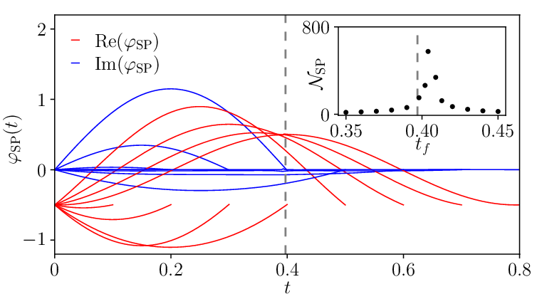
In Fig. 5 we consider the solution $\varphi_{\SP}(t|t_{f})$ of Eq. (11) as a function of the stopping time $t_{f}$ for a system initialized as $\lvert\Downarrow\rangle$ and evolved with $\Gamma=8J$. For this quench, a DQPT occurs at $t^{*}\approx 0.397$. It can be seen that the entire SP configuration evolves as a function of $t_{f}$, with an abrupt change occurring at $t_{f}\approx t^{*}$ whereby the real and imaginary parts of the SP field change sign. As shown in the inset, the number of iterations $\mathcal{N}_{\SP}$ required to recursively solve Eq. (11) sharply increases in a region near $t_{f}\approx t^{*}$. In particular, we find that the recursive solution does not converge within $10^{3}$ iterations for $0.404<t_{f}<0.409$. Such behavior points to an instability of the recursive solution in this region, which could be due to the coexistence of different minima yielding a comparable action; the leading and subleading contributions would then switch at a critical time $t^{*}_{\SP}\approx 0.406$. These observations suggest that DQPTs in $|A_{dd}|^{2}$ are associated with an abrupt change of the product-state configuration carrying the largest contribution to the quantum dynamics, consistently with recent findings De Nicola et al. 2021. This immediately generalizes the phenomenology of ground-state QPTs in the disentanglement formalism, where QPTs are associated with an abrupt change of the dominant trajectory as a function of a control parameter De Nicola 2021. Similar switching behavior near DQPTs was previously observed by considering generalized expectation values in fermionic systems Canovi et al. 2014. In the present context, this phenomenology would not be reproduced if the SP field corresponded to the mean field, since it is closely tied to the end-time dependence of Eq. (11). The full quantum dynamics, obtained from sampling, includes the additional effects of entanglement on top of the optimal SP product-state dynamics. This potentially explains the small difference between $t^{*}_{\SP}$ and the DQPT critical time $t^{*}$: the product-state approximation provided by the SP field can only determine the DQPT location approximately, as a degree of entanglement is always needed to fully capture these phenomena De Nicola et al. 2021.

In this manuscript, we have introduced an importance sampling scheme for the real-time dynamics of many-body quantum spin systems. The importance sampling method is based on the disentanglement approach, whereby unitary quantum dynamics is exactly mapped to an ensemble of classical stochastic processes. Quantum expectation values are then obtained as averages over stochastic trajectories, which can be generated numerically. We have shown that the dominant contribution to a given observable is given by a saddle point trajectory, which can be obtained by extremizing an appropriate effective action. By preferentially sampling trajectories close to the saddle point trajectory, it is possible to significantly improve the performance of the method compared to direct sampling, as we have demonstrated for both local observables and return probabilities. This improvement in performance is due to a suppression in the strength of fluctuations in the stochastic quantities, which determine the numerical efficiency of the method. However, fluctuations are still found to grow exponentially with time and the system size; while the accessible parameter regions can be extended by using importance sampling, large systems and late times remain challenging to capture. Further progress will thus be needed in order for the method to access interesting regimes of higher-dimensional quantum dynamics; several directions for development can be envisaged, including cluster approaches and the development of approximate schemes that truncate fluctuations. Since the importance sampling scheme completely eliminates fluctuations in the limit of a Hamiltonian made up of commuting terms, it would also be interesting to explore its application to higher-spin systems, where the performance of the approach might benefit from the proximity to a classical limit. Furthermore, the broader framework introduced in this work might prove useful beyond its application to importance sampling. In the context of imaginary-time evolution, it has recently been shown that corrections to the mean-field estimate for ground state expectation values can be analytically obtained order-by-order by viewing the disentanglement approach as a field theory De Nicola 2021. A similar development for real-time evolution would make it possible to systematically include the effect of entanglement on top of the leading-order mean-field dynamics.

Acknowledgments.— SDN would like to thank S. Begg, M. J. Bhaseen, B. Doyon, V. Gritsev, C. Mendl and M. Serbyn for valuable feedback and discussions. SDN acknowledges funding from the Institute of Science and Technology (IST) Austria, and from the European Union’s Horizon 2020 research and innovation programme under the Marie Skłodowska-Curie Grant Agreement No. 754411.

During the preparation of this manuscript we became aware of the work Begg et al. 2020b, in which an importance sampling scheme is developed by considering the Hermiticity of the effective Hamiltonian governing the stochastic evolution; this also leads to an improvement in the accessible time-scale for a given number of simulations.

References

- Langen et al. (2015) T. Langen, R. Geiger, and J. Schmiedmayer, Ultracold atoms out of equilibrium, Annu. Rev. Condens. Matter Phys. 6, 201 (2015).
- Gross and Bloch (2017) C. Gross and I. Bloch, Quantum simulations with ultracold atoms in optical lattices, Science 357, 995 (2017).
- Polkovnikov et al. (2011) A. Polkovnikov, K. Sengupta, A. Silva, and M. Vengalattore, Colloquium: Nonequilibrium dynamics of closed interacting quantum systems, Rev. Mod. Phys. 83, 863 (2011).
- Rigol et al. (2007) M. Rigol, V. Dunjko, V. Yurovsky, and M. Olshanii, Relaxation in a completely integrable many-body quantum system: An ab initio study of the dynamics of the highly excited states of 1d lattice hard-core bosons, Phys. Rev. Lett. 98, 050405 (2007).
- Rigol et al. (2008) M. Rigol, V. Dunjko, and M. Olshanii, Thermalization and its mechanism for generic isolated quantum systems, Nature 452, 854 (2008).
- Kinoshita et al. (2006) T. Kinoshita, T. Wenger, and D. S. Weiss, A quantum Newton’s cradle, Nature 440, 900 (2006).
- Abanin et al. (2019) D. A. Abanin, E. Altman, I. Bloch, and M. Serbyn, Colloquium: Many-body localization, thermalization, and entanglement, Rev. Mod. Phys. 91, 021001 (2019).
- Heyl (2018) M. Heyl, Dynamical quantum phase transitions: a review, Rep. Prog. Phys. 81, 054001 (2018).
- Turner et al. (2018) C. J. Turner, A. A. Michailidis, D. A. Abanin, M. Serbyn, and Z. Papić, Weak ergodicity breaking from quantum many-body scars, Nat. Phys. 14, 745 (2018).
- Else et al. (2020) D. V. Else, C. Monroe, C. Nayak, and N. Y. Yao, Discrete time crystals, Annu. Rev. Condens. Matter Phys. 11, 467 (2020).
- Calabrese et al. (2016) P. Calabrese, F. H. L. Essler, and G. Mussardo, Introduction to ‘quantum integrability in out of equilibrium systems’, J. Stat. Mech.: Theory Exp. 2016 (6), 064001.
- Vidal (2007) G. Vidal, Classical simulation of infinite-size quantum lattice systems in one spatial dimension, Phys. Rev. Lett. 98, 070201 (2007).
- Haegeman et al. (2011) J. Haegeman, J. I. Cirac, T. J. Osborne, I. Pižorn, H. Verschelde, and F. Verstraete, Time-dependent variational principle for quantum lattices, Phys. Rev. Lett. 107, 070601 (2011).
- Paeckel et al. (2019) S. Paeckel, T. Köhler, A. Swoboda, S. R. Manmana, U. Schollwöck, and C. Hubig, Time-evolution methods for matrix-product states, Ann. Phys. (N. Y.) 411, 167998 (2019).
- Schuch et al. (2007) N. Schuch, M. M. Wolf, F. Verstraete, and J. I. Cirac, Computational complexity of projected entangled pair states, Phys. Rev. Lett. 98, 140506 (2007).
- Czarnik et al. (2019) P. Czarnik, J. Dziarmaga, and P. Corboz, Time evolution of an infinite projected entangled pair state: An efficient algorithm, Phys. Rev. B 99, 035115 (2019).
- Richter et al. (2020) J. Richter, T. Heitmann, and R. Steinigeweg, Quantum quench dynamics in the transverse-field Ising model: A numerical expansion in linked rectangular clusters, SciPost Phys. 9, 31 (2020).
- Schmitt and Heyl (2020) M. Schmitt and M. Heyl, Quantum many-body dynamics in two dimensions with artificial neural networks, Phys. Rev. Lett. 125, 100503 (2020).
- Verdel et al. (2020) R. Verdel, M. Schmitt, Y.-P. Huang, P. Karpov, and M. Heyl, Variational classical networks for dynamics in interacting quantum matter (2020), arXiv:2007.16084 [cond-mat.str-el] .
- Gutiérrez and Mendl (2021) I. L. Gutiérrez and C. B. Mendl, Real time evolution with neural-network quantum states (2021), arXiv:1912.08831 [cond-mat.dis-nn] .
- Hogan and Chalker (2004) P. M. Hogan and J. T. Chalker, Path integrals, diffusion on SU(2) and the fully frustrated antiferromagnetic spin cluster, J. Phys. A: Math. Gen. 37, 11751 (2004).
- Ringel and Gritsev (2013) M. Ringel and V. Gritsev, Dynamical symmetry approach to path integrals of quantum spin systems, Phys. Rev. A 88, 062105 (2013).
- De Nicola et al. (2019) S. De Nicola, B. Doyon, and M. J. Bhaseen, Stochastic approach to non-equilibrium quantum spin systems, J. Phys. A: Math. Theor. 52, 05LT02 (2019).
- De Nicola et al. (2020) S. De Nicola, B. Doyon, and M. J. Bhaseen, Non-equilibrium quantum spin dynamics from classical stochastic processes, J. Stat. Mech.: Theory Exp. 2020 (1), 013106.
- Begg et al. (2020a) S. E. Begg, A. G. Green, and M. J. Bhaseen, Fluctuations and non-hermiticity in the stochastic approach to quantum spins, J. Phys. A: Math. Theor. 53, 50LT02 (2020a).
- Galitski (2011) V. Galitski, Quantum-to-classical correspondence and Hubbard-Stratonovich dynamical systems: A Lie-algebraic approach, Phys. Rev. A 84, 012118 (2011).
- Hubbard (1959) J. Hubbard, Calculation of partition functions, Phys. Rev. Lett. 3, 77 (1959).
- Stratonovich (1957) R. L. Stratonovich, On a method of calculating quantum distribution functions, Sov. Phys. Dokl. 2, 416 (1957).
- Wei and Norman (1963) J. Wei and E. Norman, Lie algebraic solution of linear differential equations, J. Math. Phys. 4, 575 (1963).
- Kolokolov (1986) I. Kolokolov, Functional representation for the partition function of the quantum heidenberg ferromagnet, Phys. Lett. A 114, 99 (1986).
- De Nicola (2021) S. De Nicola, Disentanglement approach to quantum spin ground states: Field theory and stochastic simulation, J. Stat. Mech.: Theory Exp. 2021 (1), 013101.
- Heyl et al. (2013) M. Heyl, A. Polkovnikov, and S. Kehrein, Dynamical quantum phase transitions in the transverse-field Ising model, Phys. Rev. Lett. 110, 135704 (2013).
- Kloeden and Platen (1992) P. E. Kloeden and E. Platen, Numerical Solution of Stochastic Differential Equations (Springer-Verlag Berlin Heidelberg, Berlin, Heidelberg, 1992).
- Rüemelin (1982) W. Rüemelin, Numerical treatment of stochastic differential equations, SIAM J. Numer. Anal. 19, 604 (1982).
- Burrage et al. (2004) K. Burrage, P. M. Burrage, and T. Tian, Numerical methods for strong solutions of stochastic differential equations: An overview, Proc. Math. Phys. Eng. Sci. 460, 373 (2004).
- Ng et al. (2013) R. Ng, E. S. Sørensen, and P. Deuar, Simulation of the dynamics of many-body quantum spin systems using phase-space techniques, Phys. Rev. B 88, 144304 (2013).
- Pfeuty (1970) P. Pfeuty, The one-dimensional Ising model with a transverse field, Ann. Phys. (N. Y.) 57, 79 (1970).
- Dirac (1930) P. A. M. Dirac, Note on exchange phenomena in the Thomas atom, Math. Proc. Camb. Philos. Soc 26, 376–385 (1930).
- Kramer (2008) P. Kramer, A review of the time-dependent variational principle, J. Phys.: Conf. Ser. 99, 012009 (2008).
- Weinberg and Bukov (2017) P. Weinberg and M. Bukov, QuSpin: a Python package for dynamics and exact diagonalisation of quantum many body systems part I: Spin chains, SciPost Phys. 2, 003 (2017).
- Jurcevic et al. (2017) P. Jurcevic, H. Shen, P. Hauke, C. Maier, T. Brydges, C. Hempel, B. P. Lanyon, M. Heyl, R. Blatt, and C. F. Roos, Direct observation of dynamical quantum phase transitions in an interacting many-body system, Phys. Rev. Lett. 119, 080501 (2017).
- Pfeuty and Elliott (1971) P. Pfeuty and R. J. Elliott, The Ising model with a transverse field. II. ground state properties, J. Phys. C: Solid State Phys. 4, 2370 (1971).
- du Croo de Jongh and van Leeuwen (1998) M. S. L. du Croo de Jongh and J. M. J. van Leeuwen, Critical behavior of the two-dimensional Ising model in a transverse field: A density-matrix renormalization calculation, Phys. Rev. B 57, 8494 (1998).
- De Nicola et al. (2021) S. De Nicola, A. A. Michailidis, and M. Serbyn, Entanglement view of dynamical quantum phase transitions, Phys. Rev. Lett. 126, 040602 (2021).
- Canovi et al. (2014) E. Canovi, P. Werner, and M. Eckstein, First-order dynamical phase transitions, Phys. Rev. Lett. 113, 265702 (2014).
- Begg et al. (2020b) S. E. Begg, A. G. Green, and M. J. Bhaseen, Time-evolving Weiss fields in the stochastic approach to quantum spins (2020b), arXiv:2011.07924 [cond-mat.str-el] .
Appendix A Functional derivatives of the disentangling variables
Here we provide the functional derivatives of the disentangling variables, which can be obtained from the SDEs (4). For clarity we suppress site indices, , since all variables at different sites are independent. Let us begin from ; differentiating the equation of motion (4a) yields