跳到论文正文
W Papers独立论文阅读器 arXiv:2103.16459 论文正文 计算阅读时间 · 0%
引用这篇论文根据当前论文元数据生成,正式投稿前建议核对。


License: CC Zero
arXiv:2103.16459v1 [math.AP] 30 Mar 2021

Loss of Regularity of Solutions to Shock Reflection Problems by a Non-symmetric Convex Wedge with Potential Flow Equations

Jingchen Hu
Abstract

In this paper, we study the problem of shock reflection by a wedge, with the potential flow equation, which is a simplification of the Euler System.

In [5] and [6], the existence theory of shock reflection problems with the potential flow equation was established, when the wedge is symmetric w.r.t. the direction of the upstream flow. As a natural extension of [5] and [6], we study non-symmetric cases, i.e. when the direction of the upstream flow forms a nonzero angle with the symmetry axis of the wedge.

The main idea of investigating the regularity of solutions to non-symmetric problems is to study the symmetry of the solution. Then difficulties arise such as free boundaries and degenerate ellipticity, especially when ellipticity degenerates on the free boundary. We developed an integral method to overcome these difficulties.

Some estimates near the corner of wedge is also established, as an extension of G.Lieberman’s work.

We proved that in non-symmetric cases, the ideal Lipschitz solution to the potential flow equation, which we call regular solution, does not exist. This suggests that the potential flow solutions to the non-symmetric shock reflection problem, should have some singularity which is not encountered in symmetric case.

1 Introduction

In [5], it was shown that with some simplifications we can reduce the shock reflection problem to a boundary value problem for a quasi-linear second order degenerate elliptic equation. And in [5] the problem is rigorously solved when the shock is reflected by a symmetric convex wedge (the symmetric axis of the wedge is perpendicular to the shock). It’s natural to ask if the existence result holds in the non-symmetric case, i.e. when the symmetric axis of the wedge is not perpendicular to the shock. To answer this question, we define regular solutions to the problem, which are characterized by reasonable physical and mathematical properties. Then we derive a contradiction from the existence of such kinds of regular solutions (Theorem 1). So this implies solutions to the non-symmetric problem should have some type or types of singularity, which is not encountered in the symmetric case.

In this section, we first derive the potential flow equation from conservation laws, then we reduce the problem to a boundary value problem in a domain with a free boundary. Then after stating the existence results and introducing some notations, we define regular solutions to the problem.

1.1 The Potential Flow Equation

In this paper we study the phenomena of plane shock reflection by a wedge. Precisely, when a plane shock, with upstream state (u1,0,ρ1)(u_{1},0;\rho_{1}) and downstream state (0,0,ρ0)(0,0;\rho_{0}), hits a wedge WW,

W={(x1,x2)∣−x1​cot⁡(σ−δ)<x2​<x1​cot⁡(σ+δ),x1>​0}W=\{(x_{1},x_{2})\mid-x_{1}\cot(\sigma-\delta)<x_{2}<x_{1}\cot(\sigma+\delta),x_{1}>0\}

it experiences a reflection-diffraction process. Here we denote the state with density ρ\rho and velocity (u,v)(u,v) by (u,v,ρ)(u,v;\rho).

Figure 1: Non-symmetric Shock Reflection-Diffraction Problem

Some mathematical models have been used in the past to study this problem, including Euler System [20] and its simplification potential flow equation [5] and [6].

In this paper we consider isentropic (p=κ​ργ,γ>0)(p=\kappa\rho^{\gamma},\gamma>0) and non-vortex(∇×(u,v)=0)(\nabla\times(u,v)=0) fluids. So the state of the fluid is governed by the density ρ\rho and a potential function Φ\Phi(∇Φ=(u,v)\nabla\Phi=(u,v)).

Our equations in (x→,t)(\vec{x},t) coordinates are

∂tρ+∇x⋅[ρ​∇xΦ]=0​ (mass conservation),\displaystyle\partial_{t}\rho+\nabla_{x}\cdot[\rho\nabla_{x}\Phi]=0\text{\ (mass conservation)}, (1)
∂tΦ+12​|∇xΦ|2+ργ−1=B0​ (Bernoulli law).\displaystyle\partial_{t}\Phi+{1\over 2}\left|\nabla_{x}\Phi\right|^{2}+\rho^{\gamma-1}=B_{0}\text{\ (Bernoulli law)}. (2)

In the equations above, ∇x=(∂x1,∂x2)\nabla_{x}=(\partial_{x^{1}},\partial_{x^{2}}). And equation (2) comes from combining the following momentum conservation equation (3) with mass conservation equation (1).

The equation of momentum conservation is

∂t(ρ∇xΦ)+∂j(ρ∂iΦ∂jΦ)∂i+∇p=0.\displaystyle\partial_{t}(\rho\nabla_{x}\Phi)+\partial_{j}(\rho\partial_{i}\Phi\partial_{j}\Phi)\partial_{i}+\nabla p=0. (3)

Combine it with mass conservation (1), we get:

∂t∇xΦ+∇x|∇xΦ|22+∇pρ=0.\partial_{t}\nabla_{x}\Phi+\nabla_{x}\frac{|\nabla_{x}\Phi|^{2}}{2}+\frac{\nabla p}{\rho}=0.

Plugging in p=κ​ργp=\kappa\rho^{\gamma}, it becomes:

∇x(∂tΦ+|∇xΦ|22+γ​κγ−1​ργ−1)=0.\nabla_{x}\left(\partial_{t}\Phi+\frac{|\nabla_{x}\Phi|^{2}}{2}+\frac{\gamma\kappa}{\gamma-1}\rho^{\gamma-1}\right)=0.

If the potential function Φ\Phi satisfies the equation above weakly on ℝ2∖W{\mathbb{R}}^{2}\setminus W, we can remove ∇x\nabla_{x} and get

∂tΦ+|∇xΦ|22+γ​κγ−1​ργ−1=B0,\displaystyle\partial_{t}\Phi+\frac{|\nabla_{x}\Phi|^{2}}{2}+\frac{\gamma\kappa}{\gamma-1}\rho^{\gamma-1}=B_{0}, (4)

where B0B_{0} is a constant independent of x,tx,t. Previously, for fixed tt, Φ\Phi is only defined up to a constant, so, if B0B_{0} depends on tt, we can extract a function of tt from B0B_{0}.

Finally, we can make κ=γ−1γ\kappa=\frac{\gamma-1}{\gamma} by the scaling,

(x→,t,B0)→(α​x→,α2​t,α−2​B0),α2=κ​γ/(γ−1),(\vec{x},t,B_{0})\rightarrow(\alpha\vec{x},\alpha^{2}t,\alpha^{-2}B_{0}),\alpha^{2}=\kappa\gamma/(\gamma-1),

and get

∂tΦ+12​|∇xΦ|2+ργ−1=B0.\displaystyle\partial_{t}\Phi+{1\over 2}\left|\nabla_{x}\Phi\right|^{2}+\rho^{\gamma-1}=B_{0}. (5)

And in front of the incident shock (u,v,ρ)=(0;ρ0)(u,v;\rho)=(0;\rho_{0}), so B0B_{0} should be ρ0γ−1.\rho_{0}^{\gamma-1}. Now we have reduced our reflection-diffraction problem to the following:

Problem 1.

Initial-boundary value problem

Find a solution of system (1) (2), in (ℝ2∖W)×ℝ≥0({{\mathbb{R}}^{2}\setminus W})\times\mathbb{R}^{\geq 0}, with B0=ρ0γ−1B_{0}=\rho_{0}^{\gamma-1}, which satisfies the initial condition

(ρ,Φ)∣t=0={(ρ0,0),for x2>x1cot(σ+δ) or x2<−x1cot(σ−δ),x1>0,(ρ1,u1​x1),for ​x1<0,(\rho,\Phi)\mid_{t=0}=\left\{\begin{array}[]{cc}(\rho_{0},0),&\text{for }x_{2}>x_{1}\cot(\sigma+\delta)\text{ or }x_{2}<-x_{1}\cot(\sigma-\delta),x_{1}>0,\\ (\rho_{1},u_{1}x_{1}),&\text{for }x_{1}<0,\end{array}\right.

and the slip boundary condition along the boundary of the wedge ∂W\partial W:

∇xΦ⋅𝕟∣∂W=0.\nabla_{x}\Phi\cdot\mathbb{n}\mid_{\partial W}=0.

This initial-boundary value problem is invariant under the self-similar scaling:

(x→,t)→(α​x→,α​t),(ρ,Φ)→(ρ,Φ/α)​for ​α>0,(\vec{x},t)\rightarrow(\alpha\vec{x},\alpha t),\ (\rho,\Phi)\rightarrow(\rho,\Phi/\alpha)\ \text{for }\alpha>0,

so we look for self-similar solutions which satisfy

ρ⁡(x→,t)=ρ⁡(ξ,η),Φ⁡(x→,t)=t​ϕ​(ξ,η)​ for ​(ξ,η)=x→/t.\rho(\vec{x},t)=\rho(\xi,\eta),\ \Phi(\vec{x},t)=t\phi(\xi,\eta)\text{ for }(\xi,\eta)=\vec{x}/t.

For self-similar solution mass conservation becomes:

∇⋅(ρ∇ϕ)−∇ρ⋅(ξ,η)=0,\displaystyle\nabla\cdot(\rho\nabla\phi)-\nabla\rho\cdot(\xi,\eta)=0, (6)

and by Bernoulli Law(2) cc, ρ\rho can be represented by:

c2=(γ−1)​ργ−1=(γ−1)​(ρ0γ−1−ϕ+ϕξ​ξ+ϕη​η−ϕξ2+ϕη22).\displaystyle c^{2}=(\gamma-1)\rho^{\gamma-1}=(\gamma-1)(\rho_{0}^{\gamma-1}-\phi+\phi_{\xi}\xi+\phi_{\eta}\eta-\frac{\phi_{\xi}^{2}+\phi_{\eta}^{2}}{2}). (7)

If we define φ=ϕ−ξ2+η22\varphi=\phi-\frac{\xi^{2}+\eta^{2}}{2}, which is named as pseudo-potential function in [5], then relations above can be written as

∇⋅(ρ∇φ)+2ρ=0,\displaystyle\nabla\cdot(\rho\nabla\varphi)+2\rho=0, (8)
c2=(γ−1)​ργ−1=(γ−1)​(ρ0γ−1−12​|∇φ|2−φ),\displaystyle c^{2}=(\gamma-1)\rho^{\gamma-1}=(\gamma-1)\left(\rho_{0}^{\gamma-1}-{1\over 2}|\nabla\varphi|^{2}-\varphi\right), (9)

where cc stands for the sonic speed. By plugging (7) into (6), the equation for ϕ\phi can also be written as

[c2−(ϕξ−ξ)2]​ϕξ​ξ−2​(ϕξ−ξ)​(ϕη−η)​ϕξ​η+[c2−(ϕη−η)2]​ϕη​η=0.\left[c^{2}-(\phi_{\xi}-\xi)^{2}\right]\phi_{\xi\xi}-2(\phi_{\xi}-\xi)(\phi_{\eta}-\eta)\phi_{\xi\eta}+\left[c^{2}-(\phi_{\eta}-\eta)^{2}\right]\phi_{\eta\eta}=0.

So the equation for ϕ\phi or φ\varphi is elliptic if and only if

|∇φ|<c.|\nabla\varphi|<c.

So now we can reduce the initial-boundary value problem in (x→,t)(\vec{x},t)-space to the following boundary value problem in self-similar (ξ,η)(\xi,\eta)-space.

Problem 2.

Boundary Value Problem

Find a weak solution φ\varphi of (8), in ℝ2∖W{\mathbb{R}}^{2}\setminus W, which satisfies Neumann boundary condition

∇φ⋅𝕟=0,on ∂W,\nabla\varphi\cdot\mathbb{n}=0,\ \ \text{on }\partial W,

and asymptotic boundary condition at infinity: when ​ξ2+η2→∞\text{when }\xi^{2}+\eta^{2}\rightarrow\infty

φ→{φ0=−12​(ξ2+η2),for ​ξ>X,η>ξ​cot⁡(σ+δ)​ or ​η<−ξ​cot⁡(σ−δ)φ1=−12​(ξ2+η2)+u1​(ξ−X),for ​ξ<X,η>0,\varphi\rightarrow\left\{\begin{array}[]{cc}\varphi_{0}=-{1\over 2}(\xi^{2}+\eta^{2}),&\text{for }\xi>X,\eta>\xi\cot(\sigma+\delta)\text{ or }\eta<-\xi\cot(\sigma-\delta)\\ \varphi_{1}=-{1\over 2}(\xi^{2}+\eta^{2})+u_{1}(\xi-X),&\text{for }\xi<X,\eta>0\end{array}\right.,

where XX is the speed of the incident shock, and is also the ξ\xi-coordinate of the incident shock in (ξ,η)(\xi,\eta)-plane.

1.2 Boundary Condition, Shock and Sonic Circle

We try to find a weak solution to the equation (8) (9), however because of the existence of shocks and sonic circles, directly solving (8) (9) is not convenient. So, based on some physical observations, we divide ℝ2∖W{{\mathbb{R}}^{2}\setminus W} into several regions, and solve equations in different regions separately.

Physical observations suggest that, on (ξ,η)(\xi,\eta)-plane, ℝ2∖W{{\mathbb{R}}^{2}\setminus W} should be divided into six regions, as illustrated by Figure 2. The fluid in each region has properties which are different from those of its neighbors. Fluids in front of the incident shock are static, they are in State(0)(0). Fluids in State(I) are the fluids behind the incident shock, its velocity and density are given as conditions. Fluids in State(II±)(\textup{II}_{\pm})have uniform velocities and densities, their velocities can be found by algebraic computations. The essential problem is to describe the behavior of the fluid in the region Ω\Omega. We solve this problem by finding a φ\varphi solving (8) and (9) in Ω\Omega and satisfying some boundary conditions on ∂Ω\partial\Omega,

Figure 2: Structures and Notations

In the following, we explain what are the conditions that should be satisfied on ∂Ω\partial\Omega. Actually these conditions are the physical conditions that should be satisfied along shocks and sonic circles.

We first consider the boundary conditions on the shock. Let Γ\Gamma be a shock on (ξ,η)(\xi,\eta)-plane, separating regions Ω+\Omega_{+} and Ω−\Omega_{-}. The potential function, velocity and density of the gas in Ω±\Omega_{\pm} are denoted by ϕ±\phi_{\pm}, (u±,v±)(u_{\pm},v_{\pm}) and ρ±\rho_{\pm} respectively.

And since this is self-similar coordinate, point (ξ,η)(\xi,\eta) on Γshock\Gamma_{\text{shock}}, will be moving with velocity (ξ,η)(\xi,\eta). So the relative velocity of point represented by (ξ,η)(\xi,\eta) and gas in Ω±\Omega_{\pm}, is (u±−ξ,v±−η)(u_{\pm}-\xi,v_{\pm}-\eta), which is ∇ϕ±−(ξ,η)\nabla\phi_{\pm}-(\xi,\eta) or ∇φ±\nabla\varphi_{\pm}, with pseudo-potential function φ±=ϕ±−ξ2+η22\varphi_{\pm}=\phi_{\pm}-{\xi^{2}+\eta^{2}\over 2}.

So Mass Conservation across shock should be

[ρ+​(∇ϕ+−(ξ,η))−ρ−​(∇ϕ−−(ξ,η))]⋅𝕟=0,[\rho_{+}(\nabla\phi_{+}-(\xi,\eta))-\rho_{-}(\nabla\phi_{-}-(\xi,\eta))]\cdot\mathbb{n}=0, (10)

or, with pseudo-potential function

(ρ+∇φ+−ρ−∇φ−)⋅𝕟=0.(\rho_{+}\nabla\varphi_{+}-\rho_{-}\nabla\varphi_{-})\cdot\mathbb{n}=0. (11)

And note that, in generic case, the normal direction of Γ\Gamma is (u+−u−,v+−v−)(u_{+}-u_{-},v_{+}-v_{-}). So (10) and (11) can also be written as

[ρ+​(∇ϕ+−(ξ,η))−ρ−​(∇ϕ−−(ξ,η))]⋅(u+−u−,v+−v−)=0,\displaystyle[\rho_{+}(\nabla\phi_{+}-(\xi,\eta))-\rho_{-}(\nabla\phi_{-}-(\xi,\eta))]\cdot(u_{+}-u_{-},v_{+}-v_{-})=0, (12)
(ρ+∇φ+−ρ−∇φ−)⋅(u+−u−,v+−v−)=0.\displaystyle(\rho_{+}\nabla\varphi_{+}-\rho_{-}\nabla\varphi_{-})\cdot(u_{+}-u_{-},v_{+}-v_{-})=0. (13)

In this paper, most of time, (10) (11) (12) (13) will all be referred to as RH condition.

And we also require vorticity vanish, so on Γ\Gamma, the tangential velocity of gas in Ω+\Omega_{+} and Ω−\Omega_{-} should be equal. This leads to the continuity assumption of potential function

ϕ+=ϕ−​(or equivalently,​φ+=φ−).\phi_{+}=\phi_{-}\ (\text{or equivalently,}\ \varphi_{+}=\varphi_{-}). (14)

(14) and any one of (10) (11) (12) (13) constitute free boundary condition on shock.

Then for convenience, we define weak solutions to the potential flow equation. Notice that free boundary condition is singular form of equation(6), which is mass conservation. So it implies that two solutions to equation (6) in two domains separated by a shock, should be considered as a global weak solution, if they satisfy equation weakly, separately in two different domains, and satisfy free boundary condition.

Assume gg is a smooth function with compact support in Ω=Ω+∪Ω−\Omega=\Omega_{+}\cup\Omega_{-}, here Ω+,Ω−\Omega_{+},\Omega_{-} are separated by an arc, which is a free boundary Γ\Gamma. φ+,φ−\varphi_{+},\varphi_{-} are defined in Ω+,Ω−\Omega_{+},\Omega_{-} respectively, satisfying (6) weakly and separately. And they satisfy free boundary condition along Γ\Gamma.

∫Ωρ(∇φ,φ)∇φ⋅∇g−2ρ(∇φ,φ)g(ρ is defined by (22),φ=φ± in Ω±)\displaystyle\int_{\Omega}\rho(\nabla\varphi,\varphi)\nabla\varphi\cdot\nabla g-2\rho(\nabla\varphi,\varphi)g\ (\rho\text{ is defined by }(\ref{sonicspeed}),\ \varphi=\varphi_{\pm}\text{ in }\Omega_{\pm})
=\displaystyle= ∫Ω+ρ(∇φ+,φ+)∇φ+⋅∇g−2ρ(∇φ+,φ+)g+∫Ω−ρ(∇φ−,φ−)∇φ−⋅∇g−2ρ(∇φ−,φ−)g\displaystyle\int_{\Omega_{+}}\rho(\nabla\varphi_{+},\varphi_{+})\nabla\varphi_{+}\cdot\nabla g-2\rho(\nabla\varphi_{+},\varphi_{+})g+\int_{\Omega_{-}}\rho(\nabla\varphi_{-},\varphi_{-})\nabla\varphi_{-}\cdot\nabla g-2\rho(\nabla\varphi_{-},\varphi_{-})g
=\displaystyle= ∫Γ(ρ(∇φ+,φ+)∇φ+−ρ(∇φ−,φ−)∇φ−)⋅𝕟g(𝕟 is outer normal of Ω+)\displaystyle\int_{\Gamma}(\rho(\nabla\varphi_{+},\varphi_{+})\nabla\varphi_{+}-\rho(\nabla\varphi_{-},\varphi_{-})\nabla\varphi_{-})\cdot\mathbb{n}g\ (\mathbb{n}\text{ is outer normal of }\Omega_{+})
=\displaystyle= 0​(by free boundary condition)\displaystyle 0\ (\text{by free boundary condition})

In this paper, speed of incident shock will be denoted as XX, so XX is also the ξ\xi-coordinate of incident shock on (ξ,η)(\xi,\eta)-plane. As stated in previous subsection, speed and density of the gas behind incident shock are denoted as u1u_{1} and ρ1\rho_{1}. They satisfy:

(X−u1)​ρ1=X​ρ0​(Mass Conservation)(X-u_{1})\rho_{1}=X\rho_{0}\ (\text{Mass Conservation}) (15)
ρ1γ−1+12​u12−u1​X=ρ0γ−1​(Bernoulli Law)\rho_{1}^{\gamma-1}+{1\over 2}u_{1}^{2}-u_{1}X=\rho_{0}^{\gamma-1}\ (\text{Bernoulli Law}) (16)

(16) comes from plugging ϕ=0,\phi=0, ϕξ=u1\phi_{\xi}=u_{1}, ξ=X\xi=X and ϕη=η=0\phi_{\eta}=\eta=0 into (7).

When shock hits a parallel wall (σ=0,δ=0\sigma=0,\delta=0 with our notation), the shock will be reflected back, leaving gas static in its wake. This is called normal reflection. We denote the static gas state behind normally reflected shock as State(II¯)(\overline{\textup{II}}). Density and sonic speed of State(II¯)(\overline{\textup{II}}) are denoted as ρ¯2\overline{\rho}_{2} and c¯2\overline{c}_{2} respectively. They satisfy

c¯22=(γ−1)​ρ¯2γ−1.\overline{c}_{2}^{2}=(\gamma-1)\overline{\rho}_{2}^{\gamma-1}. (17)

The speed of reflected shock is denoted as ZZ. ZZ and ρ¯2\overline{\rho}_{2} are determined by

ρ1​(Z+u1)=ρ¯2​Z,(Mass Conservation)\rho_{1}(Z+u_{1})=\overline{\rho}_{2}Z,\ \ \ \ \ \ \ \ \ \ \ \ (\text{Mass Conservation}) (18)
ρ0γ−1+u1​(Z+X)=ρ¯2γ−1.(Bernoulli Law)\rho_{0}^{\gamma-1}+u_{1}(Z+X)=\overline{\rho}_{2}^{\gamma-1}.\ \ \ \ \ \ \ (\text{Bernoulli Law}) (19)

There will be one and only one physically admissible solution to (18) and (19), which satisfies

ρ¯2>ρ1, or ​Z>0.\overline{\rho}_{2}>\rho_{1},\text{ or }Z>0.

And by argument in section 3.1 of [5], we know

c¯22>Z2.\overline{c}_{2}^{2}>Z^{2}. (20)

We will denote c¯22−Z2=Y\sqrt{\overline{c}_{2}^{2}-Z^{2}}=Y, so (−Z,Y)(-Z,Y) is the coordinate of point, where reflected shock intersects sonic circle.

When incident shock is not parallel to the wall (σ=0,δ≠0\sigma=0,\delta\neq 0, with our notation), a two-shock structure will form. And this is called the regular reflection, contrary to the Mach reflection, which is more complicated.

Two regular reflections occur in our case, one is above ξ\xi-axis, another is below ξ\xi-axis. They are denoted as State(II+)(\textup{II}_{+}) and State​(II−)\text{State}(\textup{II}_{-}). The density and velocity of State(II±)(\textup{II}_{\pm}) are denoted as ρ2±\rho_{2}^{\pm} and (u2±,v2±)(u_{2}^{\pm},v_{2}^{\pm}) respectively. When σ\sigma is small enough, the ρ2±\rho_{2}^{\pm} and (u2±,v2±)(u_{2}^{\pm},v_{2}^{\pm}), satisfying ρ2±>ρ\rho_{2}^{\pm}>\rho are uniquely determined, as shown in section 3.1 of [5]. And analysis in [5] also shows or implies

  • •

    u2+>0,v2+>0;u2−>0,v2−<0u_{2}^{+}>0,\ v_{2}^{+}>0;\ u_{2}^{-}>0,\ v_{2}^{-}<0;

  • •

    |u2+|+|v2+|+|u2−|+|v2−|≤Cp​σ|u_{2}^{+}|+|v_{2}^{+}|+|u_{2}^{-}|+|v_{2}^{-}|\leq C_{p}\sigma;

  • •

    |ρ2+−ρ¯2|+|ρ2−−ρ¯2|≤Cp​σ|\rho_{2}^{+}-\overline{\rho}_{2}|+|\rho_{2}^{-}-\overline{\rho}_{2}|\leq C_{p}\sigma.

1.3 Symmetric Case

Figure 3: Symmetric Case

In [5], when the wedge is symmetric (δ=0)(\delta=0) and σ\sigma is very small, solutions to boundary value problem was rigorously constructed. Later, more general existence results, without requiring σ\sigma being small, was proved in [6]. In the remaining part of this subsection for the convenience of notation, we denote the region surrounded by arc A1​A2A_{1}A_{2}, A2​A3A_{2}A_{3}…Ai​Ai+1A_{i}A_{i+1}…Ak​A1A_{k}A_{1} by region A1​A2​…​AkA_{1}A_{2}...A_{k}. And arc A1​A2​…​AkA_{1}A_{2}...A_{k} means arc A1​A2∪A2​A3∪…​Ak−1​AkA_{1}A_{2}\cup A_{2}A_{3}\cup...A_{k-1}A_{k}.

When solving the problem in the symmetric case, many difficulties arise, including free boundary problems and ellipticity degeneration, especially when ellipticity degenerates on free boundary. To overcome these difficulties many new techniques were developed in [5] and [6].In [5], they first showed the existence of State(II)(\textup{II}), based on implicit function theorem, when the wedge is close to a half-plane(σ\sigma closes to zero). Then in region P1​P2​P3​P4P_{1}P_{2}P_{3}P_{4} they constructed φ\varphi as a solution to equation (8) (9) with the following boundary condition:

φ𝕟=0, on arc ​P2​P3​P4,φ=φ2, on arc ​P1​P4,φ=φ1, on arc ​P1​P2,(ρ∇φ−ρ1∇φ1)⋅𝕟=0,on arc ​P1​P2.\begin{array}[]{cc}\varphi_{\mathbb{n}}=0,&\text{ \ on arc }P_{2}P_{3}P_{4},\\ \varphi=\varphi_{2},&\text{ on arc }P_{1}P_{4},\\ \varphi=\varphi_{1},&\text{ on arc }P_{1}P_{2},\\ (\rho\nabla\varphi-\rho_{1}\nabla\varphi_{1})\cdot\mathbb{n}=0,&\text{on arc }P_{1}P_{2}.\end{array}

Notice that, in above, arc P1​P2P_{1}P_{2} is a free boundary so we can pose two boundary conditions on it. And arc P1​P4P_{1}P_{4} is a part of the sonic circle of State(II)(\textup{II})

P1​P4⊂{(ξ,η)∣|ξ−u2|2+|η−v2|2=c22}.P_{1}P_{4}\subset\left\{(\xi,\eta)\mid|\xi-u_{2}|^{2}+|\eta-v_{2}|^{2}=c_{2}^{2}\right\}.

Along it, equation degenerates. And for the solution they constructed, ∇φ=∇φ2\nabla\varphi=\nabla\varphi_{2} on arc P1​P4P_{1}P_{4}.

If we extend the definition of φ\varphi to the whole ℝ2∖W{\mathbb{R}}^{2}\setminus W, by defining

φ={φ0,in {ξ>ξ0}∖Wφ1,in {ξ≤ξ0}∖(W∪region P0P1P2P3)φ2,in region ​P0​P1​P4\varphi=\left\{\begin{array}[]{cc}\varphi_{0},&\text{in }\{\xi>\xi_{0}\}\setminus W\\ \varphi_{1},&\text{in }\{\xi\leq\xi_{0}\}\setminus(W\cup\text{region }P_{0}P_{1}P_{2}P_{3})\\ \varphi_{2},&\text{in }\text{region }P_{0}P_{1}P_{4}\end{array}\right.

then φ\varphi is a weak solution to Problem 2.

So a natural question is can we solve the boundary value problem for non-symmetric case? And if so, can the solution be as regular as the solution constructed in [5]?

1.4 Notations

Before presenting the result of this paper, we introduce some notations and conventions. Notations introduced here will be universally used through out the paper, except Appendix. Some other notations, which will only be used in a specific section (or subsection), will be introduced later, in the corresponding sections.

In (ξ,η)(\xi,\eta)-plane, we still use WW to denote the wedge. State(I) is the state left to shock (behind incident shock and in front of reflected shock), and State(II¯){(\overline{\textup{II}})} denotes the state behind normal reflected shock. Since now we have two regular shock reflections, we use State(II+\textup{II}_{+}) denotes the state above ξ\xi-axis, and use State(II−\textup{II}_{-}) denotes the state below ξ\xi-axis. And State(0)(0) is the state in front of (or right to) incident shock.

Γsonic±{\Gamma_{\text{sonic}}}^{\pm} denotes the sonic circle of State(II±\textup{II}_{\pm}), and Γsonic\Gamma_{\text{sonic}} denotes their union. Γshock\Gamma_{\text{shock}} denotes the part of reflected shock between Γsonic+\Gamma_{\text{sonic}}^{+} and Γsonic−\Gamma_{\text{sonic}}^{-}. And Γshock+\Gamma_{\text{shock}}^{+} is used to denote the part of reflected shock above Γsonic+\Gamma_{\text{sonic}}^{+}. While Γshock−\Gamma_{\text{shock}}^{-} is used to denote the part of reflected shock below Γsonic−\Gamma_{\text{sonic}}^{-}. Γwedge+\Gamma_{\text{wedge}}^{+}(Γwedge−\Gamma_{\text{wedge}}^{-}) denotes upper(lower) part of boundary of wedge, while Γwedge\Gamma_{\text{wedge}} denotes the union of these two rays.

𝒞\mathcal{C} denotes corner of wedge. Ω\Omega denotes the region surrounded by Γshock\Gamma_{\text{shock}}, Γsonic\Gamma_{\text{sonic}} and Γwedge\Gamma_{\text{wedge}}. CpC_{p} is a constant depends only on physical constants, ρ1,u1,ρ0,γ\rho_{1},u_{1},\rho_{0},\gamma.

And, for convenience, we may choose different directions for wedge and flow in different parts of this paper, like illustrated in the following pictures. But the angle between symmetry axis of wedge and direction of flow will always be denoted as δ\delta. So in every section we declare either direction of flow or direction of wedge.

Figure 4: Non-Vertical Shock hits Symmetric Wedge
Figure 5: Vertical Shock hits Non-Symmetric Wedge
Refer to caption
Figure 6: Γwedge+\Gamma_{\text{wedge}}^{+} coincides with +η+\eta-Axis
Refer to caption
Figure 7: A position easy to compute RH condition at PP

1.5 Regular Solutions and the Conclusion of the Paper

In this subsection the direction of the wedge and the flow is shown in Figure 7, s.t. the symmetry axis of the wedge is ξ\xi-axis.

Definition 1.

Regular Solution for Shock Reflection

We define that a regular solution of self-similar shock reflection problem is a function ϕ∈C3​(Ω¯∖(Γsonic¯∪𝒞))∩C1​(Ω¯∖𝒞)∩L​i​p​(Ω¯)\phi\in C^{3}(\overline{\Omega}\setminus(\overline{\Gamma_{\text{sonic}}}\cup\mathcal{C}))\cap C^{1}(\overline{\Omega}\setminus\mathcal{C})\cap Lip(\overline{\Omega}) which satisfies the following conditions:

Equation
[c2−(ϕξ−ξ)2]​ϕξ​ξ−2​(ϕξ−ξ)​(ϕη−η)​ϕξ​η+[c2−(ϕη−η)2]​ϕη​η=0​, in Ω,\left[c^{2}-(\phi_{\xi}-\xi)^{2}\right]\phi_{\xi\xi}-2(\phi_{\xi}-\xi)(\phi_{\eta}-\eta)\phi_{\xi\eta}+\left[c^{2}-(\phi_{\eta}-\eta)^{2}\right]\phi_{\eta\eta}=0\text{, in $\Omega$,} (21)

where,

c2=(γ−1)​ργ−1=(γ−1)​(ρ0γ−1−ϕ+ϕξ​ξ+ϕη​η−|∇ϕ|22),c^{2}=(\gamma-1)\rho^{\gamma-1}=(\gamma-1)\left(\rho_{0}^{\gamma-1}-\phi+\phi_{\xi}\xi+\phi_{\eta}\eta-\frac{|\nabla\phi|^{2}}{2}\right), (22)

and equivalently if we define φ=ϕ−ξ2+η22\varphi=\phi-\frac{\xi^{2}+\eta^{2}}{2}, relations above can be written as

∇⋅[ρ∇φ]+2ρ=0,in Ω,\nabla\cdot[\rho\nabla\varphi]+2\rho=0,\ \text{in $\Omega$},

where,

c2=(γ−1)​ργ−1=(γ−1)​(ρ0γ−1−12​|∇φ|2−φ);c^{2}=(\gamma-1)\rho^{\gamma-1}=(\gamma-1)\left(\rho_{0}^{\gamma-1}-{1\over 2}|\nabla\varphi|^{2}-\varphi\right);
Subsonic Condition
|∇φ|2<c2​, in ​Ω¯∖Γsonic¯;|\nabla\varphi|^{2}<c^{2}\text{, in }\overline{\Omega}\setminus\overline{\Gamma_{\text{sonic}}}; (23)
Continuity Conditions on Sonic Circles
ϕ=ϕ2±, on Γsonic±,\phi=\phi_{2}^{\pm},\ \ \text{ on $\Gamma_{\text{sonic}}^{\pm}$}, (24)
∇ϕ=∇ϕ2±, on Γsonic±;\nabla\phi=\nabla\phi_{2}^{\pm},\ \ \text{ on $\Gamma_{\text{sonic}}^{\pm}$}; (25)
Free Boundary Conditions on the Shock (Non-Vorticity and RH Condition)
φ=φ1,[ρ1∇φ1−ρ∇φ]⋅𝕟=0, on Γshock,\displaystyle\varphi=\varphi_{1},\ \ \ [\rho_{1}\nabla\varphi_{1}-\rho\nabla\varphi]\cdot\mathbb{n}=0,\text{ on }\Gamma_{\text{shock}}, (26)

or equivalently,

ϕ=ϕ1,[ρ1(u1cosδ−ξ,u1sinδ−η)−ρ(u−ξ,v−η)]⋅𝕟=0, on Γshock;\phi=\phi_{1},\ \ \ [\rho_{1}(u_{1}\cos\delta-\xi,u_{1}\sin\delta-\eta)-\rho(u-\xi,v-\eta)]\cdot\mathbb{n}=0,\text{ on }\Gamma_{\text{shock}}; (27)
Slip (or Neumann) Boundary Condition on the Boundary of Wedge
ϕ𝕟=0​, on ​Γwedge;\phi_{\mathbb{n}}=0\text{, on }\Gamma_{\text{wedge}}; (28)
Regularity Assumption of Shock
Γshock\Gamma_{\text{shock}} is not tangential to the direction of the upcoming flow at any point, and it’s a C1C^{1} curve up to its ends; (29)
Admissible Condition
ρ1<ρ​, in ​Ω¯.\rho_{1}<\rho\text{, in }\overline{\Omega}. (30)

If we can find such a regular solution ϕ\phi, then we can combine it with potential functions of State(I)(\textup{I}), State(II±)(\textup{II}_{\pm}) and State(0)(0) to form a function from ℝ2∖W{\mathbb{R}}^{2}\setminus W to ℝ{\mathbb{R}}, which will be a weak solution to Problem 2.

In this paper we prove

Theorem 1 (Main Theorem).

For isentropic gases (with c2=(γ−1)​ργ−1c^{2}=(\gamma-1)\rho^{\gamma-1}), given a vertical shock with the upstream state (u1,0,ρ1)(u_{1},0;\rho_{1}) and the downstream state (0,0,ρ0)(0,0;\rho_{0}), we can find ϵT>0\epsilon_{T}>0 small enough, which depends on ρ0,ρ1,u1\rho_{0},\rho_{1},u_{1} and γ\gamma, s.t. when the shock hits a convex wedge, with vertex angle π−2​σ​(0<σ<ϵT)\pi-2\sigma(0<\sigma<\epsilon_{T}) and if the symmetry axis of the wedge forms an angle δ⁡(0<δ≤σ)\delta(0<\delta\leq\sigma) with the direction of the upstream flow, the shock reflection problem does not have a regular solution as defined in Definition 1.

1.6 Structure of the Paper

Section 2 provides some relatively rough estimates. Some of these estimates are used to show more regularities of regular solution, some of them imply that when σ\sigma tends to zero, our corresponding regular solution tends to potential function of normal reflection which is a constant.

With these estimates, we can have a good control on regular solution in later sections.

In section 3, with computation we show precisely how geometric structure differs from symmetric shock reflection. And so we can tell the relative position of Γsonic+\Gamma_{\text{sonic}}^{+} and Γsonic−~\widetilde{\Gamma_{\text{sonic}}^{-}}, here Γsonic−~\widetilde{\Gamma_{\text{sonic}}^{-}} is the reflection of Γsonic−{\Gamma_{\text{sonic}}^{-}} across symmetry axis of wedge. And the geometric structure will be useful when doing integral by parts in section 4. The technique in this section depends on comparison of derivatives, at δ\delta or σ=0\sigma=0, so it’s only available for σ\sigma and δ\delta small.

In section 4, we proved “symmetric estimate”. It says, if we take the symmetry axis of wedge as ξ\xi-axis, regular solution is almost symmetric w.r.t. η\eta, precisely, near symmetry axis of wedge,

|ϕ⁡(ξ,η)−ϕ⁡(ξ,−η)|≤Cp​δ.|\phi(\xi,\eta)-\phi(\xi,-\eta)|\leq C_{p}\delta.

To prove above, we first get an integral type symmetric estimate. With method of [7] we are able to control ∫Ω∩Ω~|ϕ−ϕ~|3\int_{\Omega\cap\widetilde{\Omega}}|\phi-\tilde{\phi}|^{3} by a divergence integral, so we can reduce it to integral on boundary of Ω∩Ω~\Omega\cap\widetilde{\Omega}, then making use of RH condition and ∇ϕ=∇ϕ2±\nabla\phi=\nabla\phi_{2}^{\pm} on Γsonic±\Gamma_{\text{sonic}}^{\pm}, we can further transform boundary integral into integral in Ω​△​Ω~\Omega\triangle\widetilde{\Omega} and on ∂(Ω∪Ω~)\partial(\Omega\cup\widetilde{\Omega}). These integrals can either be estimated with the properties of R​HRH function derived in section 2, or by explicit computation and boundary condition.

Then we get L∞L^{\infty} symmetric estimate near corner of wedge, with Moser iteration; and around where shock intersects symmetry axis, with a generalized Krylov-Safonov estimate (Lemma B.1). From this L∞L^{\infty} estimate, we get on symmetry axis of wedge, |ϕη|≤Cp​δ|\phi_{\eta}|\leq C_{p}\delta near shock and |ϕη|≤Cp​δ​rα2−1|\phi_{\eta}|\leq C_{p}\delta r^{{\alpha\over 2}-1} near corner of wedge.

Above gradient estimates will be used in section 5, to control boundary integral.

In section 5, we provided a lower bound for ϕ−ϕ~\phi-\widetilde{\phi}, precisely:

ϕ⁡(ξ,η)−ϕ⁡(ξ,−η)≥δ⁡(ηCp−Cp​σ13)\phi(\xi,\eta)-\phi(\xi,-\eta)\geq\delta({\eta\over C_{p}}-C_{p}\sigma^{1\over 3}) (31)

So contrary to section 4, we call this estimate as “antisymmetric estimate”. To prove above, roughly speaking, we minus a linear function η​sin⁡δ\eta\sin\delta from ϕ\phi, and denote the new function as ψ\psi, then estimate ψ⁡(ξ,−η)−ψ⁡(ξ,η)\psi(\xi,-\eta)-\psi(\xi,\eta) from above. We first do the integral estimate as in last section, then with Moser Iteration we get an L∞L^{\infty} estimate on ∂Br0\partial B_{r_{0}}, r0r_{0} is smaller then some physical constants, decided in Lemma A.1 and A.3.

With (31), we can use Lemma A.3 to get a contradiction.

In appendix are some lemmas about linear partial differential equations.

Lemma A.1 A.2 and A.3 are all about the solution of linear elliptic partial differential equation with singular coefficients near a corner. Lemma A.1 is a maximum principle, Lemma A.2 is an estimate based on conformal mapping, it gives a singular bound on |ϕη||\phi_{\eta}| and Lemma A.3 implies that out of a convex wedge, a C1C^{1} solution to our linear partial differential equation, should not be C1,αC^{1,\alpha}, if solution is bigger on one side of the symmetry axis of wedge.

Lemma B.1 is a generalized Krylov-Safonov estimate, which is used to get L∞L^{\infty}-symmetric estimate near free boundary.

2 Fundamental Estimates for Regular Solutions

In this section, we provide some fundamental estimates for regular solutions defined in Definition 1. Roughly speaking, with estimates in this section we have a better control on regular solution.

  • •

    We show the shock reflection corresponds to our regular solution is close to normal shock reflection (subsection2.3),

  • •

    we provide some regularity estimate of potential function (subsection 2.1, 2.9, 2.10, 2.11)

  • •

    we provide a “coercive” estimate of the RH function, in subsection 2.5, which will be used in section 4 and section 5 to estimate boundary integral.

2.1 Continuity of Velocity at the Corner of the Wedge

Based on Estimate in [4], a regular solution to potential flow equation, which is only assumed to be Lipschitz at corner of wedge should actually be C1C^{1}. And so at corner of wedge,

ϕξ=u=ϕη=v=0\phi_{\xi}=u=\phi_{\eta}=v=0. (32)

We cannot immediately get |∇ϕ|​(ξ,η)≤Cp​(|ξ|+|η|)α|\nabla\phi|(\xi,\eta)\leq C_{p}(|\xi|+|\eta|)^{\alpha}, which is contained in Proposition 3, because now we don’t have any control on |∇ϕ|0|\nabla\phi|_{0} in Ω¯\overline{\Omega}. We will more precisely estimate ∇ϕ\nabla\phi until section 2.9.

2.2 Comparison of ϕ\phi and ϕ1\phi_{1}

In this subsection, position of wedge and flow is as shown in Figure 7, so velocity of upstream flow is (u1,0)(u_{1},0). And we want to show ϕ<ϕ1\phi<\phi_{1} in Ω\Omega.

First, in Ω\Omega, ϕ\phi satisfies (21). In this paper, except Appendix, when we only use linear property of (21), we denote this linear equation by

ai​j​ϕi​j=0.a_{ij}\phi_{ij}=0. (33)

ai​j′​s{a_{ij}}^{\prime}s are polynomials of ξ,η,u,v\xi,\eta,u,v, so ai​j∈C1​(Ω¯∖(Γsonic¯∪𝒞))a_{ij}\in C^{1}(\overline{\Omega}\setminus(\overline{\Gamma_{\text{sonic}}}\cup\mathcal{C})).

So,

ai​j​(ϕ−ϕ1)i​j=ai​j​ϕi​j=0,a_{ij}(\phi-\phi_{1})_{ij}=a_{ij}\phi_{ij}=0, (34)

since ϕ1\phi_{1} is a linear function. So

ϕ−ϕ1 cannot achieve maximum in Ω.\text{$\phi-\phi_{1}$ cannot achieve maximum in $\Omega$}. (35)

Then, on Γsonic±\Gamma_{\text{sonic}}^{\pm},

ϕ−ϕ1​=(24)​ϕ2±−ϕ1.\phi-\phi_{1}\underset{(\ref{continuityofpotentialfunctiononsoniccircle})}{=}\phi_{2}^{\pm}-\phi_{1}.

Since in section 1.2, we have shown that ϕ1=ϕ2±\phi_{1}=\phi_{2}^{\pm} on Γshock±\Gamma_{\text{shock}}^{\pm}, and when σ\sigma small enough |∇ϕ2±|≤Cp​σ|\nabla\phi_{2}^{\pm}|\leq C_{p}\sigma, so on right-hand side of Γshock±\Gamma_{\text{shock}}^{\pm}

ϕ2,ξ±<ϕ1,ξ=u1,(providing σ small enough)\phi^{\pm}_{2,\xi}<\phi_{1,\xi}=u_{1},\ \text{(providing $\sigma$ small enough)}

and so

ϕ=ϕ2±<ϕ1​ on Γsonic±.\phi=\phi_{2}^{\pm}<\phi_{1}\text{ on $\Gamma_{\text{sonic}}^{\pm}$.} (36)

For 𝕟±=(cos⁡(σ±δ),∓sin⁡(σ±δ))\mathbb{n}_{\pm}=(\cos(\sigma\pm\delta),\mp\sin(\sigma\pm\delta)), which are outer unit normal vectors of Ω\Omega on Γwedge±\Gamma_{\text{wedge}}^{\pm},

(ϕ−ϕ1)𝕟±=ϕ𝕟±−ϕ1,𝕟±=−u1​cos⁡(σ±δ)<0,on Γwedge± (providing σ small enough)(\phi-\phi_{1})_{\mathbb{n}_{\pm}}=\phi_{\mathbb{n}_{\pm}}-\phi_{1,\mathbb{n}_{\pm}}=-u_{1}\cos(\sigma\pm\delta)<0,\ \text{on $\Gamma_{\text{wedge}}^{\pm}$}\text{\ (providing $\sigma$ small enough)}

So,

ϕ−ϕ1 cannot achieve maximum on Γwedge±.\text{$\phi-\phi_{1}$ cannot achieve maximum on ${\Gamma_{\text{wedge}}^{\pm}}$}. (37)

Note, that at corner of wedge when Γwedge+¯\overline{\Gamma_{\text{wedge}}^{+}} meets Γwedge−¯\overline{\Gamma_{\text{wedge}}^{-}}, we can apply both 𝕟+\mathbb{n}_{+} and 𝕟−\mathbb{n}_{-} to ϕ\phi.

Combine (34) (35) (36) (37) and (26) together, we get

ϕ<ϕ1​, in ​Ω\phi<\phi_{1}\text{, in }\Omega (38)

2.3 Gradient Estimates

In this subsection the direction of upcoming flow is (u1,0)(u_{1},0), as shown in Figure 7.

Take ξ−\xi-derivative of linear equation of ϕ\phi, (33), we get:

a11​uξ​ξ+2​a12​uξ​η+a22​uη​η+a22​(a11a22)ξ​uξ+a22​(2​a12a22)ξ​uη=0.a_{11}u_{\xi\xi}+2a_{12}u_{\xi\eta}+a_{22}u_{\eta\eta}+a_{22}(\frac{a_{11}}{a_{22}})_{\xi}u_{\xi}+a_{22}(\frac{2a_{12}}{a_{22}})_{\xi}u_{\eta}=0. (39)
So uu can’t achieve maximum(or minimum) in Ω∘\Omega^{\circ} . (40)

If at some interior point of Γwedge+\Gamma_{\text{wedge}}^{+}, uu achieves a local maximum (or minimum), then at this point,

u𝕥=0,D𝕥​(ϕ𝕟)=0,ai​j​ϕi​j=0.u_{{\mathbb{t}}}=0,\ D_{{\mathbb{t}}}(\phi_{\mathbb{n}})=0,\ a_{ij}\phi_{ij}=0.

In above 𝕥=(sin⁡(σ+δ),cos⁡(σ+δ)),𝕟=(cos⁡(σ+δ),−sin⁡(σ+δ)){\mathbb{t}}=(\sin(\sigma+\delta),\cos(\sigma+\delta)),\ \mathbb{n}=(\cos(\sigma+\delta),-\sin(\sigma+\delta)), write above equations in matrix form:

(sin⁡(σ+δ)cos⁡(σ+δ)0sin⁡(σ+δ)​cos⁡(σ+δ)cos2⁡(σ+δ)−sin2⁡(σ+δ)−sin⁡(σ+δ)​cos⁡(σ+δ)a112​a12a22)​(uξuηvη)=0.\left(\begin{array}[]{ccc}\sin(\sigma+\delta)&\cos(\sigma+\delta)&0\\ \sin(\sigma+\delta)\cos(\sigma+\delta)&\cos^{2}(\sigma+\delta)-\sin^{2}(\sigma+\delta)&-\sin(\sigma+\delta)\cos(\sigma+\delta)\\ a_{11}&2a_{12}&a_{22}\end{array}\right)\left(\begin{array}[]{c}u_{\xi}\\ u_{\eta}\\ v_{\eta}\end{array}\right)=0.

Determinant of this 3×33\times 3 matrix equals

−sin⁡(σ+δ)​[a11​cos2⁡(σ+δ)−2​a12​sin⁡(σ+δ)​cos⁡(σ+δ)+a22​sin2⁡(σ+δ)]≠0.-\sin(\sigma+\delta)[a_{11}\cos^{2}(\sigma+\delta)-2a_{12}\sin(\sigma+\delta)\cos(\sigma+\delta)+a_{22}\sin^{2}(\sigma+\delta)]\neq 0.

This implies at this maximum point ∇u=0\nabla u=0, which is a contradiction to Hopf lemma.

So uu can’t achieve maximum(or minimum) value at any interior point of Γwedge+\Gamma_{\text{wedge}}^{+}. (41)
Similarly, when σ≠δ\sigma\neq\delta, uu can’t achieve any maximum(or minimum) value on Γwedge−\Gamma_{\text{wedge}}^{-}, (42)
 and when σ=δ, u=0 on Γwedge−.\text{ and when $\sigma=\delta$, $u=0$ on $\Gamma_{\text{wedge}}^{-}$}. (43)

On Γshock\Gamma_{\text{shock}}, ϕ−ϕ1=0\phi-\phi_{1}=0 (26); in Ω\Omega, ϕ−ϕ1<0\phi-\phi_{1}<0 (38),

ai​j​(ϕ−ϕ1)i​j=0​(because ϕ1 is a linear function),a_{ij}(\phi-\phi_{1})_{ij}=0\ \text{(because $\phi_{1}$ is a linear function),}

and since we know now Γshock\Gamma_{\text{shock}} is the graph of a C1C^{1} function of η\eta (29), so we can apply Hopf maximum principle, to ϕ−ϕ1\phi-\phi_{1}, and get

u=ϕξ<ϕ1,ξ=u1,on ​Γshock−Γsonic±¯.u=\phi_{\xi}<\phi_{1,\xi}=u_{1},\ \text{on }\Gamma_{\text{shock}}-\overline{\Gamma_{\text{sonic}}^{\pm}}. (44)

Put (32) (40) (41) (42) (43) (44) together, and use the assumption, that regular solution is C1C^{1} on sonic circle, we have : when σ,δ\sigma,\delta small enough s.t. u2±<u1u_{2}^{\pm}<u_{1},

u<u1,in​Ω¯.u<u_{1},\ \text{in}\ \overline{\Omega}. (45)

Now with (45) we can define S=vu1−uS=\frac{v}{u_{1}-u} in Ω¯\overline{\Omega}, and since ϕ∈C1​(Ω¯)∩C3​(Ω¯∖(Γ¯sonic∪𝒞))\phi\in C^{1}(\overline{\Omega})\cap C^{3}(\overline{\Omega}\setminus(\overline{\Gamma}_{\text{sonic}}\cup\mathcal{C})) and |u|=|u2±|<u1|u|=|u_{2}^{\pm}|<u_{1} on Γsonic±\Gamma_{\text{sonic}}^{\pm}, S∈C0​(Ω¯)∩C2​(Ω¯∖(Γsonic¯∪𝒞))S\in C^{0}(\overline{\Omega})\cap C^{2}(\overline{\Omega}\setminus(\overline{\Gamma_{\text{sonic}}}\cup\mathcal{C})).

In Ω¯∖(Γsonic¯∪𝒞)\overline{\Omega}\setminus(\overline{\Gamma_{\text{sonic}}}\cup\mathcal{C}), we have

{Sξ=Su​uξ+Sv​vξSη=Su​uη+Sv​vηa11​ϕξ​ξ+2​a12​ϕξ​η+a22​ϕη​η=0\left\{\begin{array}[]{c}S_{\xi}=S_{u}u_{\xi}+S_{v}v_{\xi}\\ S_{\eta}=S_{u}u_{\eta}+S_{v}v_{\eta}\\ a_{11}\phi_{\xi\xi}+2a_{12}\phi_{\xi\eta}+a_{22}\phi_{\eta\eta}=0\end{array}\right.

Solve above equation of uξ,vξ,vηu_{\xi},v_{\xi},v_{\eta}, we get (we know Sv=1u1−uS_{v}=\frac{1}{u_{1}-u} is also well defined and Sv≠0S_{v}\neq 0)

(uξvξvη)=1a11​Sv2−2​a12​Su​Sv+a22​Su2​(Su​a22−2​Sv​a12−Sv​a22a11​SvSu​a22−a11​Su−2​Su​a12+Sv​a11)​(SξSη).\displaystyle\left(\begin{array}[]{c}u_{\xi}\\ v_{\xi}\\ v_{\eta}\end{array}\right)={1\over a_{11}S_{v}^{2}-2a_{12}S_{u}S_{v}+a_{22}S_{u}^{2}}\left(\begin{array}[]{cc}S_{u}a_{22}-2S_{v}a_{12}&-S_{v}a_{22}\\ a_{11}S_{v}&S_{u}a_{22}\\ -a_{11}S_{u}&-2S_{u}a_{12}+S_{v}a_{11}\end{array}\right)\left(\begin{array}[]{c}S_{\xi}\\ S_{\eta}\end{array}\right).

Plug

a11​uξ​ξ+2​a12​uξ​η+a22​uη​η+a22​(a11a22)ξ​uξ+a22​(2​a12a22)ξ​uη=0a_{11}u_{\xi\xi}+2a_{12}u_{\xi\eta}+a_{22}u_{\eta\eta}+a_{22}(\frac{a_{11}}{a_{22}})_{\xi}u_{\xi}+a_{22}(\frac{2a_{12}}{a_{22}})_{\xi}u_{\eta}=0
a11​vξ​ξ+2​a12​vξ​η+a22​vη​η+a11​(a22a11)η​vη+a11​(2​a12a11)η​vξ=0,a_{11}v_{\xi\xi}+2a_{12}v_{\xi\eta}+a_{22}v_{\eta\eta}+a_{11}(\frac{a_{22}}{a_{11}})_{\eta}v_{\eta}+a_{11}(\frac{2a_{12}}{a_{11}})_{\eta}v_{\xi}=0,

into:

a11​Sξ​ξ+2​a12​Sξ​η+a22​Sη​η\displaystyle a_{11}S_{\xi\xi}+2a_{12}S_{\xi\eta}+a_{22}S_{\eta\eta}
=\displaystyle= a11​(Su​uξ​ξ+Sv​vξ​ξ+Su​u​uξ2+2​Su​v​uξ​vξ+Sv​v​vξ2)\displaystyle a_{11}(S_{u}u_{\xi\xi}+S_{v}v_{\xi\xi}+S_{uu}u_{\xi}^{2}+2S_{uv}u_{\xi}v_{\xi}+S_{vv}v_{\xi}^{2})
+2​a12​(Su​uξ​η+Sv​vξ​η+Su​u​uξ​uη+Su​v​uξ​vη+Su​v​uη​vξ+Sv​v​vξ​vη)\displaystyle+2a_{12}(S_{u}u_{\xi\eta}+S_{v}v_{\xi\eta}+S_{uu}u_{\xi}u_{\eta}+S_{uv}u_{\xi}v_{\eta}+S_{uv}u_{\eta}v_{\xi}+S_{vv}v_{\xi}v_{\eta})
+a22​(Su​uη​η+Sv​vη​η+Su​u​uη2+2​Su​v​uη​vη+Sv​v​vη2)\displaystyle+a_{22}(S_{u}u_{\eta\eta}+S_{v}v_{\eta\eta}+S_{uu}u_{\eta}^{2}+2S_{uv}u_{\eta}v_{\eta}+S_{vv}v_{\eta}^{2})

and replace uξ,vξ=uη,vηu_{\xi},v_{\xi}=u_{\eta},v_{\eta} by linear combination of Sξ,SηS_{\xi},S_{\eta}, using (2.3). We get there exists b^i′​s\hat{b}_{i}^{\prime}s, which are C0C^{0} functions in Ω¯∖(Γsonic¯∪𝒞)\overline{\Omega}\setminus(\overline{\Gamma_{\text{sonic}}}\cup\mathcal{C}), s.t.

ai​j​Si​j+b^i​Si=0.a_{ij}S_{ij}+\hat{b}_{i}S_{i}=0. (54)
So SS can’t achieve maximum or minimum at interior point of Ω\Omega. (55)

To show that SS can not achieve maximum or minimum on Γshock\Gamma_{\text{shock}} either, we define

R​H=[ρ⁡(u−ξ,v−η)−ρ1​(u1−ξ,−η)]​(u−u1,v), in Ω¯RH=[\rho(u-\xi,v-\eta)-\rho_{1}(u_{1}-\xi,-\eta)](u-u_{1},v),\text{ in $\overline{\Omega}$} (56)

in the expression above,

ρ=[ρ0γ−1−ϕ+ϕξ​ξ+ϕη​η−ϕξ2+ϕη22]1γ−1\rho=\left[\rho_{0}^{\gamma-1}-\phi+\phi_{\xi}\xi+\phi_{\eta}\eta-\frac{\phi_{\xi}^{2}+\phi_{\eta}^{2}}{2}\right]^{1\over\gamma-1} (57)

R​HRH can be considered either as a function of ξ,η\xi,\eta or a function of five variables, ϕ,u,v,ξ,η\phi,u,v,\xi,\eta, as expressed in (56) and (57). To avoid confusion, when RH is considered as a function of five variables, ξ⁡(η​ and ​T)\xi(\eta\text{ and }T)-derivative of RH will be denoted as R​H(ξ)​(R​H(η)​ and ​R​H(T))RH_{(\xi)}(RH_{(\eta)}\text{ and }RH_{(T)}) respectively. Taking tangential derivative of RH on Γshock\Gamma_{\text{shock}} gives:

R​HT=R​Hu​uT+R​Hv​vT+R​Hϕ​ϕT+R​H(T)(here ​T=(v,u1−u)),RH_{T}=RH_{u}u_{T}+RH_{v}v_{T}+RH_{\phi}\phi_{T}+RH_{(T)}\ \ (\text{here }T=(v,u_{1}-u)), (58)
  • •

    on left-hand side of (58), RH is considered as a pure function of ξ,η\xi,\eta,

  • •

    on right-hand side of (58), RH is considered as a function of ϕ,u,v,ξ,η\phi,u,v,\xi,\eta.

Then algebraic computation gives, when RH is considered as a function of ϕ,u,v,ξ,η\phi,u,v,\xi,\eta:

R​Hϕ=−[(u−ξ)​(u−u1)+(v−η)​v]​ρ2−γγ−1,RH_{\phi}=-[(u-\xi)(u-u_{1})+(v-\eta)v]\frac{\rho^{2-\gamma}}{\gamma-1},
R​H(ξ)=(ρ1−ρ)​(u−u1)+[(u−ξ)​(u−u1)+(v−η)​v]​ρ2−γγ−1​u,RH_{(\xi)}=(\rho_{1}-\rho)(u-u_{1})+[(u-\xi)(u-u_{1})+(v-\eta)v]\frac{\rho^{2-\gamma}}{\gamma-1}u,
R​H(η)=v⁡(ρ1−ρ)+[(u−ξ)​(u−u1)+(v−η)​v]​ρ2−γγ−1​v.RH_{(\eta)}=v(\rho_{1}-\rho)+[(u-\xi)(u-u_{1})+(v-\eta)v]\frac{\rho^{2-\gamma}}{\gamma-1}v.

Combine these with

ϕT=u​v+(u1−u)​v=u1​v,\phi_{T}=uv+(u_{1}-u)v=u_{1}v,

and RH condition, we know on right-hand side of (58)

R​Hϕ​ϕT+R​H(T)=0.RH_{\phi}\phi_{T}+RH_{(T)}=0.

So along Γshock\Gamma_{\text{shock}}

0=R​HT=R​Hu​uT+R​Hv​vT.0=RH_{T}=RH_{u}u_{T}+RH_{v}v_{T}. (59)

If SS achieves maximum or minimum at some interior point of Γshock\Gamma_{\text{shock}}, at this point:

DT​S=Su​uT+Sv​vT=0,D_{T}S=S_{u}u_{T}+S_{v}v_{T}=0, (60)

We put (60) (59) and linear equation of ϕ\phi (33) together in matrix form:

(R​Hu​vR​Hv​v+R​Hu​(u1−u)R​Hv​(u1−u)Su​vSv​v+Su​(u1−u)Sv​(u1−u)a112​a12a22)​(uξvξvη)=0.\left(\begin{array}[]{ccc}RH_{u}v&RH_{v}v+RH_{u}(u_{1}-u)&RH_{v}(u_{1}-u)\\ S_{u}v&S_{v}v+S_{u}(u_{1}-u)&S_{v}(u_{1}-u)\\ a_{11}&2a_{12}&a_{22}\end{array}\right)\left(\begin{array}[]{c}u_{\xi}\\ v_{\xi}\\ v_{\eta}\end{array}\right)=0.

Plug Su=v(u1−u)2,Sv=1u1−uS_{u}=\frac{v}{(u_{1}-u)^{2}},S_{v}=\frac{1}{u_{1}-u} into the 3×33\times 3 matrix above, with computation we get its determinant is

−(R​Hu​(u−u1)+R​Hv​v)​(a11−2​a12​vu1−u+a22​v2(u1−u)2)\displaystyle-(RH_{u}(u-u_{1})+RH_{v}v)(a_{11}-2a_{12}\frac{v}{u_{1}-u}+a_{22}\frac{v^{2}}{(u_{1}-u)^{2}})
≤\displaystyle\leq −ρ⁡[(u−u1)2+v2]​(1−(u−ξ)2+(v−η)2c2)​(a11−2​a12​vu1−u+a22​v2(u1−u)2)<0\displaystyle-\rho[(u-u_{1})^{2}+v^{2}](1-\frac{(u-\xi)^{2}+(v-\eta)^{2}}{c^{2}})(a_{11}-2a_{12}\frac{v}{u_{1}-u}+a_{22}\frac{v^{2}}{(u_{1}-u)^{2}})<0

So at such minimum or maximum point, D2​ϕ=0,S𝕟=0D^{2}\phi=0,\ S_{\mathbb{n}}=0, which contradicts with Hopf lemma, since SS satisfies (54) in Ω\Omega.

So S can not achieve a minimum or maximum at any interior point of Γshock.\text{So $S$ can not achieve a minimum or maximum at any interior point of $\Gamma_{\text{shock}}$}. (61)

Then if SS achieves maximum or minimum at some interior point of Γwedge+\Gamma_{\text{wedge}}^{+}, at this point we have:

D𝕥​ϕ𝕟=0,D𝕥​S=0,a11​ϕξ​ξ+2​a12​ϕξ​η+a22​ϕη​η=0,D_{\mathbb{t}}\phi_{\mathbb{n}}=0,\ D_{\mathbb{t}}S=0,\ a_{11}\phi_{\xi\xi}+2a_{12}\phi_{\xi\eta}+a_{22}\phi_{\eta\eta}=0,

in above 𝕥=(sin⁡(σ+δ),cos⁡(σ+δ)){\mathbb{t}}=(\sin(\sigma+\delta),\cos(\sigma+\delta)), again we write them in matrix form:

(sin⁡(σ+δ)​cos⁡(σ+δ)cos2⁡(σ+δ)−sin2⁡(σ+δ)−sin⁡(σ+δ)​cos⁡(σ+δ)Su​sin⁡(σ+δ)Sv​sin⁡(σ+δ)+Su​cos⁡(σ+δ)Sv​cos⁡(σ+δ)a112​a12a22)​(uξvξvη)=0,\left(\begin{array}[]{ccc}\sin(\sigma+\delta)\cos(\sigma+\delta)&\cos^{2}(\sigma+\delta)-\sin^{2}(\sigma+\delta)&-\sin(\sigma+\delta)\cos(\sigma+\delta)\\ S_{u}\sin(\sigma+\delta)&S_{v}\sin(\sigma+\delta)+S_{u}\cos(\sigma+\delta)&S_{v}\cos(\sigma+\delta)\\ a_{11}&2a_{12}&a_{22}\end{array}\right)\left(\begin{array}[]{c}u_{\xi}\\ v_{\xi}\\ v_{\eta}\end{array}\right)=0,

with computation we get the determinant of the 3×33\times 3 matrix above is:

(a11​cos2⁡(σ+δ)−2​a12​sin⁡(σ+δ)​cos⁡(σ+δ)+a22​sin2⁡(σ+δ))​(Sv​cos⁡(σ+δ)+Su​sin⁡(σ+δ))\displaystyle(a_{11}\cos^{2}(\sigma+\delta)-2a_{12}\sin(\sigma+\delta)\cos(\sigma+\delta)+a_{22}\sin^{2}(\sigma+\delta))(S_{v}\cos(\sigma+\delta)+S_{u}\sin(\sigma+\delta))
=\displaystyle= (a11​cos2⁡(σ+δ)−2​a12​sin⁡(σ+δ)​cos⁡(σ+δ)+a22​sin2⁡(σ+δ))​u1​cos⁡(σ+δ)(u1−u)2>0.\displaystyle(a_{11}\cos^{2}(\sigma+\delta)-2a_{12}\sin(\sigma+\delta)\cos(\sigma+\delta)+a_{22}\sin^{2}(\sigma+\delta))\frac{u_{1}\cos(\sigma+\delta)}{(u_{1}-u)^{2}}>0.

In above we used D𝕟​ϕ=v​sin⁡(σ+δ)−u​cos⁡(σ+δ)=0D_{\mathbb{n}}\phi=v\sin(\sigma+\delta)-u\cos(\sigma+\delta)=0. Again we get at such a maximum(or minimum) point D2​ϕ=0,D^{2}\phi=0, so D𝕟​S=0D_{\mathbb{n}}S=0, which is a contradiction to Hopf lemma. With same method we can show SS cannot achieve maximum or minimum on (Γwedge−)∘(\Gamma_{\text{wedge}}^{-})^{\circ}

Combine with (61), we know SS can only achieve maximum or minimum on Γsonic¯∪𝒞\overline{\Gamma_{\text{sonic}}}\cup\mathcal{C}, so

−Cp​σ≤v2−u1−u2−<S=vu1−u<v2+u1−u2+≤Cp​σ, in ​Ω.\displaystyle-C_{p}\sigma\leq\frac{v_{2}^{-}}{u_{1}-u_{2}^{-}}<S=\frac{v}{u_{1}-u}<\frac{v_{2}^{+}}{u_{1}-u_{2}^{+}}\leq C_{p}\sigma,\text{ in }\Omega. (62)

(62) implies, providing σ\sigma small enough, if 𝕟=(n1,n2)\mathbb{n}=(n_{1},n_{2}) is the unit normal direction of Γshock\Gamma_{\text{shock}}, pointing rightward, then

n1>12,|n2|≤Cp​σ.\displaystyle n_{1}>{1\over 2},|n_{2}|\leq C_{p}\sigma. (63)

This implies,

1|slope of ​Γshock|≤Cp​σ,{1\over\left|\text{slope of }\Gamma_{\text{shock}}\right|}\leq C_{p}\sigma, (64)

so,

Γshock\Gamma_{\text{shock}} stays in a Cp​σC_{p}\sigma neighborhood of normal reflected shock. (65)

And (64) (29) also implies

Γshock\Gamma_{\text{shock}} is a C1C^{1} function of η\eta, (66)

in any of 4 positions shown in Figure 7, 7, 7 and 7. Plug (63) into R​HRH condition:

[ρ⁡(u−ξ,v−η)−ρ1​(u1−ξ,−η)]​(n1,n2)=0,[\rho(u-\xi,v-\eta)-\rho_{1}(u_{1}-\xi,-\eta)](n_{1},n_{2})=0,

we get,

|ρ⁡(u−ξ)−ρ1​(u1−ξ)|≤Cp​σ​ρ​|v−η|+Cp≤Cp​σ​ρ​(u1−u)+Cp​σ​ρ+Cp,|\rho(u-\xi)-\rho_{1}(u_{1}-\xi)|\leq C_{p}\sigma\rho|v-\eta|+C_{p}\\ \leq C_{p}\sigma\rho(u_{1}-u)+C_{p}\sigma\rho+C_{p},

so,

(1−Cp​σ)​ρ​u≥ρ⁡(ξ−Cp)−Cp,(1-C_{p}\sigma)\rho u\geq\rho(\xi-C_{p})-C_{p},

which implies:

u≥−Cp​, on ​Γshock,\displaystyle u\geq{-C_{p}}\text{, on }\Gamma_{\text{shock}}, (67)

since ρ≥ρ1\rho\geq\rho_{1}. Combining (67) with |vu1−u|<Cp​σ|\frac{v}{u_{1}-u}|<C_{p}\sigma (62), and u<u1u<u_{1} (45), gives

|v|<Cp​σ.|v|<C_{p}\sigma. (68)
Figure 8: Graph of RR

Now with estimate of vv in hand we want to get a same level estimate of uu, to do so, we define:

R⁡(u)=ρ¯2​Z−(ρ¯2γ−1−u​Z−u22)1γ−1​(u+Z),\displaystyle R(u)=\overline{\rho}_{2}Z-(\overline{\rho}_{2}^{\gamma-1}-uZ-\frac{u^{2}}{2})^{1\over\gamma-1}(u+Z), (69)

here, −Z-Z is the ξ\xi-coordinate of normal reflected shock, ρ¯2\overline{\rho}_{2} is the density of normal shock reflection.

ρ¯2​Z=ρ1​(u1+Z)\displaystyle\overline{\rho}_{2}Z=\rho_{1}(u_{1}+Z) (70)

is the RH condition for normal shock reflection.

ρ0γ−1−ϕ¯2=ρ¯2γ−1\displaystyle\rho_{0}^{\gamma-1}-\overline{\phi}_{2}=\overline{\rho}_{2}^{\gamma-1} (71)

is Bernoulli law for normal reflection.
Now in (57), replacing ρ0\rho_{0} by ρ¯2\overline{\rho}_{2} with (71) gives on Γshock\Gamma_{\text{shock}}

(ρ¯2γ−1+ϕ¯2−ϕ1+u​ξ+v​η−u2+v22)1γ−1=ρ\left(\overline{\rho}_{2}^{\gamma-1}+\overline{\phi}_{2}-\phi_{1}+u\xi+v\eta-\frac{u^{2}+v^{2}}{2}\right)^{1\over\gamma-1}=\rho (72)

Since we know , |u|≤Cp|u|\leq C_{p} (45) (67), |v|≤Cp​σ|v|\leq C_{p}\sigma (68), ϕ=ϕ1\phi=\phi_{1} on Γshock\Gamma_{\text{shock}}(26) and Γshock\Gamma_{\text{shock}} is close to normal reflected shock (65), we can estimate

ρ¯2γ−1−u​Z−u22=ργ−1+O⁡(σ).\overline{\rho}_{2}^{\gamma-1}-uZ-\frac{u^{2}}{2}=\rho^{\gamma-1}+O(\sigma). (73)

(73) implies: first, that

ρ¯2γ−1−u​Z−u22>ρ1γ−1−Cp​σ>ρ1γ−12(providing σ small enough)\overline{\rho}_{2}^{\gamma-1}-uZ-\frac{u^{2}}{2}>\rho_{1}^{\gamma-1}-C_{p}\sigma>\frac{\rho_{1}^{\gamma-1}}{2}\ \ (\text{providing $\sigma$ small enough}) (74)

so R⁡(u)R(u) is well defined; second,

ρ≤Cp​, on Γshock.\rho\leq C_{p}\text{, on $\Gamma_{\text{shock}}$.} (75)

With (63) and (68), we can reduce RH condition on Γshock\Gamma_{\text{shock}}

[ρ⁡(u−ξ,v−η)−ρ1​(u1−ξ,−η)]​(n1,n2)=0,[\rho(u-\xi,v-\eta)-\rho_{1}(u_{1}-\xi,-\eta)](n_{1},n_{2})=0,

to

|ρ⁡(u−ξ)−ρ1​(u1−ξ)|≤Cp​σ.|\rho(u-\xi)-\rho_{1}(u_{1}-\xi)|\leq C_{p}\sigma.

Plug in (65) (73) and (70), and use (75), RH condition can be further reduced to

|R⁡(u)|=|(ρ¯2γ−1−u​Z−u22)1γ−1​(u+Z)−ρ¯2​Z|≤Cp​σ|R(u)|=\left|\left(\overline{\rho}_{2}^{\gamma-1}-uZ-\frac{u^{2}}{2}\right)^{1\over\gamma-1}(u+Z)-\overline{\rho}_{2}Z\right|\leq C_{p}\sigma (76)

When u<−Zu<-Z, R⁡(u)≥ρ¯2​ZR(u)\geq\overline{\rho}_{2}Z. So with estimate (76), we know on Γshock\Gamma_{\text{shock}}, u>−Zu>-Z. And we also know u<u1u<u_{1} (45), so on Γshock\Gamma_{\text{shock}},

−Z<u<u1.-Z<u<u_{1}. (77)

Then for convenience, define

m⁡(u)=ρ¯2γ−1−u​Z−u22.m(u)=\overline{\rho}_{2}^{\gamma-1}-uZ-\frac{u^{2}}{2}.

And denote the range of uu on Γshock\Gamma_{\text{shock}} by ℛ\mathcal{R}, precisely let ℛ\mathcal{R} be the minimal subset of ℝ\mathbb{R} s.t. for every point p∈p\inΓshock\Gamma_{\text{shock}}, u⁡(p)∈ℛu(p)\in\mathcal{R}. Since uu is continuous on Γshock\Gamma_{\text{shock}}, ℛ\mathcal{R} is a connected interval. And (77) equals ℛ⊂[−Z,u1]\mathcal{R}\subset[-Z,u_{1}].

d​Rd​u\displaystyle\frac{dR}{du} =m2−γγ−1γ−1​(u+Z)2−m1γ−1\displaystyle=\frac{m^{2-\gamma\over\gamma-1}}{\gamma-1}(u+Z)^{2}-m^{1\over\gamma-1}
=m2−γγ−1γ−1​((u+Z)2−(γ−1)​m)\displaystyle=\frac{m^{2-\gamma\over\gamma-1}}{\gamma-1}((u+Z)^{2}-(\gamma-1)m)

so

(γ−1)​d​Rd​u​mγ−2γ−1=γ+12​(u+Z)2−(γ−1)​Z22−(γ−1)​ρ¯2γ−1(\gamma-1)\frac{dR}{du}m^{\gamma-2\over\gamma-1}=\frac{\gamma+1}{2}(u+Z)^{2}-\frac{(\gamma-1)Z^{2}}{2}-(\gamma-1)\overline{\rho}_{2}^{\gamma-1}

is a monotone function of uu on ℛ\mathcal{R}, and

d​Rd​u​(0)=ρ¯2γ−1γ−1​(Z2−ρ¯2γ−1​(γ−1))​<(20)−1Cp.\frac{dR}{du}(0)=\frac{\overline{\rho}^{\gamma-1}_{2}}{\gamma-1}(Z^{2}-\overline{\rho}_{2}^{\gamma-1}(\gamma-1))\underset{(\ref{subsonicityofnormallyreflectedshock})}{<}-{1\over C_{p}}.

So on [−Z,0],R′<−1Cp[-Z,0],\ R^{\prime}<-{1\over C_{p}}. Since RR is a smooth function of uu and m⁡(u)>1Cpm(u)>{1\over C_{p}} (74),

|d2​Rd​u2|≤Cp,\left|\frac{d^{2}R}{du^{2}}\right|\leq C_{p},

so there exists δ0≥1Cp,\delta_{0}\geq{1\over C_{p}}, s.t.

R′<−1Cp​ on [0,δ0] ⇒R⁡(δ0)<−1Cp.R^{\prime}<{-1\over C_{p}}\text{ on $[0,{\delta_{0}}]$ }\Rightarrow R(\delta_{0})<{-1\over C_{p}}.

And by (20) and (73):

(γ−1)​m​(u)−(u+Z)2−(η−v)2≥−Cp​σ(\gamma-1)m(u)-(u+Z)^{2}-(\eta-v)^{2}\geq-C_{p}\sigma
⇒d​Rd​u=[(u+Z)2−(γ−1)​m]​m2−γγ−1γ−1≤Cp​σ.\Rightarrow\frac{dR}{du}=\left[(u+Z)^{2}-(\gamma-1)m\right]\frac{m^{2-\gamma\over\gamma-1}}{\gamma-1}\leq C_{p}\sigma.

This means if we choose σ\sigma small enough, then R<−1CpR<-{1\over C_{p}} on (δ0,u1)({\delta_{0}},u_{1}).

And so u∈[−Z,δ0]u\in[-Z,\delta_{0}], and in this interval, Ru≤−1CpR_{u}\leq{-1\over C_{p}}. Since |R|≤Cp​σ|R|\leq C_{p}\sigma (76) and R⁡(0)=0R(0)=0,

|u|<Cp​σ​, in ​Ω.|u|<C_{p}\sigma\text{, in }\Omega. (78)

Then plug (78) into (73) we get

|ρ−ρ¯2|≤Cp​σ​, in ​Ω.|\rho-\overline{\rho}_{2}|\leq C_{p}\sigma\text{, in }\Omega. (79)

So, we have reached conclusion of this subsection:

Proposition 1.

If there is a regular solution ϕ\phi, as defined in Definition 1, then the physical state of gas, described by this potential function, is close to that of normal shock reflection, precisely

|u|+|v|+|ρ−ρ¯2|≤Cp​σ,in ​Ω,|u|+|v|+|\rho-\overline{\rho}_{2}|\leq C_{p}\sigma,\ \text{in }\Omega,

and Γshock\Gamma_{\text{shock}} stays in a Cp​σC_{p}\sigma neighborhood of normal reflected shock.

2.4 Monotonicity of the Potential Function along Some Direction

In this subsection we first rotate wedge together with flow, such that upper part of Γwedge\Gamma_{\text{wedge}} is +η+\eta-axis, as illustrated in Figure 7. Later we need to change direction of wedge and flow.

We denote:

u^1=u1​cos⁡(σ+δ),v^1=u1​sin⁡(σ+δ)\hat{u}_{1}=u_{1}\cos(\sigma+\delta),\ \ \hat{v}_{1}=u_{1}\sin(\sigma+\delta)

So the direction of upstream flow is (u^1,v^1)(\hat{u}_{1},\ \hat{v}_{1}).

First we want to show uu cannot achieve minimum at any interior point of Γshock\Gamma_{\text{shock}}.

If uu achieves minimum at some interior point on Γshock\Gamma_{\text{shock}}, then at this point (denoted by MM),

uξ>0.{u_{\xi}>0}. (80)

This is because uu satisfies a linear elliptic equation (39), Γshock\Gamma_{\text{shock}} is a C1C^{1} curve (Assumption (29)), and |1slope of shock|≤Cp​σ\left|\frac{1}{\text{slope of shock}}\right|\leq C_{p}\sigma (64), so we can apply Hopf maximum principle to uu at MM.

At this minimum point of uu we should also have

uT=0, here ​T=(v−v^1,u^1−u),u_{T}=0,\text{\ here }T=(v-\hat{v}_{1},\hat{u}_{1}-u), (81)

We put uξu_{\xi}, (81) (33) together in matrix form:

(100v−v^1u^1−u0a112​a12a22)​(uξuηvη)=(uξ00)\left(\begin{array}[]{ccc}1&0&0\\ v-\hat{v}_{1}&\hat{u}_{1}-u&0\\ a_{11}&2a_{12}&a_{22}\end{array}\right)\left(\begin{array}[]{c}u_{\xi}\\ u_{\eta}\\ v_{\eta}\end{array}\right)=\left(\begin{array}[]{c}u_{\xi}\\ 0\\ 0\end{array}\right)

Solve above linear equation of (uξ,uη,vη)(u_{\xi},u_{\eta},v_{\eta}), we get

(uξ,uη,vη)=uξ​(1,v−v^1u−u^1,−a11a22−2​a12a22​v−v^1u−u^1)\left(u_{\xi},u_{\eta},v_{\eta}\right)=u_{\xi}\left(1,\frac{v-\hat{v}_{1}}{u-\hat{u}_{1}},-\frac{a_{11}}{a_{22}}-2\frac{a_{12}}{a_{22}}\frac{v-\hat{v}_{1}}{u-\hat{u}_{1}}\right) (82)

Then we can compute the sign of

DT​S^=DT​(v−v^1u^1−u),( here, we define ​S^=v−v^1u^1−u)D_{T}\hat{S}=D_{T}(\frac{v-\hat{v}_{1}}{\hat{u}_{1}-u}),\ (\text{ here, we define }\hat{S}=\frac{v-\hat{v}_{1}}{\hat{u}_{1}-u})

Plug (82) and

 S^u=v−v^1(u^1−u)2,S^v=1u^1−u,\text{ }\hat{S}_{u}=\frac{v-\hat{v}_{1}}{(\hat{u}_{1}-u)^{2}},\ \hat{S}_{v}=\frac{1}{\hat{u}_{1}-u},

into:

DT​S^=S^u​uξ​(v−v^1)+S^v​vξ​(v−v^1)+S^u​uη​(u^1−u)+S^v​vη​(u^1−u)D_{T}\hat{S}=\hat{S}_{u}u_{\xi}(v-\hat{v}_{1})+\hat{S}_{v}v_{\xi}(v-\hat{v}_{1})+\hat{S}_{u}u_{\eta}(\hat{u}_{1}-u)+\hat{S}_{v}v_{\eta}(\hat{u}_{1}-u)

we get

DT​S^=uξ​(−S^2+2​a12a22​S^−a11a22)<0D_{T}\hat{S}=u_{\xi}\left(-\hat{S}^{2}+2\frac{a_{12}}{a_{22}}\hat{S}-\frac{a_{11}}{a_{22}}\right)<0

This means at this minimum point of uu, shock bends against upstream flow direction, as shown in Figure 9. So the tangent line lTl_{T} of Γshock\Gamma_{\text{shock}} at M, must separate domain Ω\Omega into three parts, and when we slide this line leftwards it must contact domain Ω\Omega at some interior point of Γshock\Gamma_{\text{shock}} (denote this point by NN).

Refer to caption
Figure 9: Sliding Tangent Line

Then we compare these two points MM and NN. For convenience, denote ∂ξϕ=u,∂ηϕ=v\partial_{\xi}\phi=u,\partial_{\eta}\phi=v and ρ,ξ,η\rho,\ \xi,\ \eta at M,NM,N will be denoted as uM,vM,ρM,ξM,ηMu_{M},v_{M},\rho_{M},\xi_{M},\eta_{M} and uN,vN,ρN,ξN,ηNu_{N},v_{N},\rho_{N},\xi_{N},\eta_{N} respectively.

We define

k≜v^1−vMu^1−uM=v^1−vNu^1−uN.k\triangleq\frac{\hat{v}_{1}-v_{M}}{\hat{u}_{1}-u_{M}}=\frac{\hat{v}_{1}-v_{N}}{\hat{u}_{1}-u_{N}}.

And direct computation shows

uM+k​vM\displaystyle u_{M}+kv_{M}
=\displaystyle= uM+k⁡(−k​u^1+k​uM+v^1)\displaystyle u_{M}+k(-k\hat{u}_{1}+ku_{M}+\hat{v}_{1})
≤\displaystyle\leq uN+k⁡(−k​u^1+k​uN+v^1)\displaystyle u_{N}+k(-k\hat{u}_{1}+ku_{N}+\hat{v}_{1})
=\displaystyle= uN+k​vN.\displaystyle u_{N}+kv_{N}.

Now we rotate wedge and flow s.t. lTl_{T} parallels to η\eta-axis.

For simplicity, after this rotation we still use notation in previous part of this subsection. So we still have

∂ξϕ⁡(M)=uM≤∂ξϕ⁡(N)=uN.\partial_{\xi}\phi(M)=u_{M}\leq\partial_{\xi}\phi(N)=u_{N}. (83)

Since, now, the tangent lines at M,NM,N are vertical, RH condition becomes

ρ1​(u^1−ξM)=ρM​(uM−ξM);ρ1​(u^1−ξN)=ρN​(uN−ξN).\rho_{1}(\hat{u}_{1}-\xi_{M})=\rho_{M}(u_{M}-\xi_{M});\ \ \rho_{1}(\hat{u}_{1}-\xi_{N})=\rho_{N}(u_{N}-\xi_{N}). (84)

Plugging state parameters of State(I) into (22), gives at MM and NN

ρ0γ−1=ρ1γ−1+ϕ1−u^1​ξ−v^1​η+u^12+v^122=ργ−1+ϕ−u​ξ−v​η+u2+v22.\displaystyle\rho_{0}^{\gamma-1}=\rho_{1}^{\gamma-1}+\phi_{1}-\hat{u}_{1}\xi-\hat{v}_{1}\eta+{\hat{u}_{1}^{2}+\hat{v}_{1}^{2}\over 2}=\rho^{\gamma-1}+\phi-u\xi-v\eta+{u^{2}+v^{2}\over 2}. (85)

Since at M,NM,N, v^1=v\hat{v}_{1}=v and ϕ1=ϕ\phi_{1}=\phi, (85) can be reduced to

ργ−1=ρ1γ−1+u^122−(u^1−u)​ξ−u22.\displaystyle\rho^{\gamma-1}=\rho_{1}^{\gamma-1}+\frac{\hat{u}_{1}^{2}}{2}-(\hat{u}_{1}-u)\xi-\frac{u^{2}}{2}. (86)

Then plug (86) into (84), we get at M,NM,N

−(ρ1γ−1+u^122−u^1​ξ+u​ξ−u22)1γ−1​(u−ξ)+ρ1​(u^1−ξ)=0.-(\rho_{1}^{\gamma-1}+\frac{\hat{u}_{1}^{2}}{2}-\hat{u}_{1}\xi+u\xi-{u^{2}\over 2})^{1\over\gamma-1}(u-\xi)+\rho_{1}(\hat{u}_{1}-\xi)=0.

Define:

R⁡(u,ξ)=−(ρ1γ−1+u^122−u^1​ξ+u​ξ−u22)1γ−1​(u−ξ)+ρ1​(u^1−ξ),R(u,\xi)=-(\rho_{1}^{\gamma-1}+\frac{\hat{u}_{1}^{2}}{2}-\hat{u}_{1}\xi+u\xi-{u^{2}\over 2})^{1\over\gamma-1}(u-\xi)+\rho_{1}(\hat{u}_{1}-\xi),

then R⁡(uM,ξM)=R⁡(uN,ξN)=0R(u_{M},\xi_{M})=R(u_{N},\xi_{N})=0.

Ru=−ρ⁡[1−(ξ−u)2(γ−1)​ργ−1]=−ρ⁡[1−(ξ−u)2c2]<0,R_{u}=-\rho\left[1-\frac{(\xi-u)^{2}}{(\gamma-1)\rho^{\gamma-1}}\right]=-\rho\left[1-\frac{(\xi-u)^{2}}{c^{2}}\right]<0,

Inequality above follows from (20). Note that the rotation we did in later part of this section didn’t move shock much, since we have estimated |u|,|v|≤Cp​σ|u|,|v|\leq C_{p}\sigma (78) (68), so Γshock\Gamma_{\text{shock}} still stays in a Cp​σC_{p}\sigma neighborhood of Γshock\Gamma_{\text{shock}}, after the rotation.

So when uu closes to 00 and ξ\xi closes to −Z-Z we can consider uu as a function of ξ\xi, s.t. R⁡(u⁡(ξ),ξ)=0R(u(\xi),\xi)=0. And since

Rξ=−ρ2−γγ−1​(−u^1+u)​(u−ξ)+ρ−ρ1>0,R_{\xi}=-\frac{\rho^{2-\gamma}}{\gamma-1}(-\hat{u}_{1}+u)(u-\xi)+\rho-\rho_{1}>0,

we get ∂ξu>0\partial_{\xi}u>0, which implies uM>uNu_{M}>u_{N}, and contradicts with uM≤uNu_{M}\leq u_{N}(83).

This means the minimum of uu cannot be achieved at any interior point of Γshock\Gamma_{\text{shock}}.

Now we rotate back to the position used at the beginning of this subsection.

Argument in section 2.3 shows uu cannot achieve its minimum in Ω\Omega and at interior point of Γwedge−\Gamma_{\text{wedge}}^{-}. So

u≥minΓsonic+∪Γsonic−∪Γwedge+​u=min⁡{u2+=0,u2−,0}=0u\geq\underset{\Gamma_{\text{sonic}}^{+}\cup\Gamma_{\text{sonic}}^{-}\cup\Gamma_{\text{wedge}}^{+}}{\min}u=\min\{u_{2}^{+}=0,u_{2}^{-},0\}=0 (87)

Similar argument works when we rotate wedge, s.t. Γwedge−\Gamma_{\text{wedge}}^{-} coincides with η\eta axis, so we get the following conclusion of this subsection:

Proposition 2.

Let T±T_{\pm} denote the tangent vector of Γwedge±\Gamma_{\text{wedge}}^{\pm} respectively, with T+T_{+} pointing upwards and T−T_{-} pointing downwards. If a vector 𝛄{\boldsymbol{\gamma}} satisfies

𝜸⋅T±≥0,{\boldsymbol{\gamma}}\cdot T_{\pm}\geq 0,

then,

ϕ𝜸≥0,in​Ω¯,\phi_{{\boldsymbol{\gamma}}}\geq 0,\ \text{in}\ \overline{\Omega},

for any regular solution ϕ\phi.

2.5 Estimates of the RH function

In this subsection, at first, the direction is chosen s.t. the upstream flow is (u1,0)(u_{1},0), as illustrated in Figure 7, later for convenience we will need to change the direction of wedge and flow.
Consider

G=R​H−(ρ−ρ1)​(ϕ1−ϕ)G=RH-(\rho-\rho_{1})(\phi_{1}-\phi) (88)

In subsection 2.3, RH is defined (56) (57). And we stated there, that RH can be considered either as a function of ξ,η\xi,\eta or a function of five variables u,v,ϕ,ξ,ηu,v,\phi,\xi,\eta, and when considered as a 5-variable- function, ξ⁡(η)\xi(\eta)-derivative of RH is denoted as R​H(ξ)​(R​H(η))RH_{(\xi)}(RH_{(\eta)}) respectively. Here we adopt the idea and notation.

Pure algebraic computation gives:

Gϕ=R​Hϕ+(ρ−ρ1)+(ϕ1−ϕ)​ρ2−γγ−1G_{\phi}=RH_{\phi}+(\rho-\rho_{1})+(\phi_{1}-\phi)\frac{\rho^{2-\gamma}}{\gamma-1} (89)
G(ξ)=R​H(ξ)−(ρ−ρ1)​u1−(ϕ1−ϕ)​ρ2−γγ−1​uG_{(\xi)}=RH_{(\xi)}-(\rho-\rho_{1})u_{1}-(\phi_{1}-\phi)\frac{\rho^{2-\gamma}}{\gamma-1}u (90)

Plug (89) and (90) into

Gξ=Gu​uξ+Gv​vξ+Gϕ​u+G(ξ),G_{\xi}=G_{u}u_{\xi}+G_{v}v_{\xi}+G_{\phi}u+G_{(\xi)}, (91)

we find, on right-hand side of (91), Gϕ​u+G(ξ)G_{\phi}u+G_{(\xi)} disappeared. So (91) can be reduced to

Gξ=Gu​uξ+Gv​vξ.G_{\xi}=G_{u}u_{\xi}+G_{v}v_{\xi}. (92)

And replace ξ\xi by η\eta, we get

Gη=Gu​uη+Gv​vη.G_{\eta}=G_{u}u_{\eta}+G_{v}v_{\eta}. (93)

Given σ\sigma small enough

Gu\displaystyle G_{u} =R​Hu−(ϕ1−ϕ)​ρu\displaystyle=RH_{u}-(\phi_{1}-\phi)\rho_{u}
<ρ​u1​((ξ−u)2c2−1)+(ρ1−ρ)​(ξ+Z)−u1​(ξ+Z)​ρc2​(ξ−u)+Cp​σ\displaystyle<\rho u_{1}\left(\frac{(\xi-u)^{2}}{c^{2}}-1\right)+(\rho_{1}-\rho)(\xi+Z)-u_{1}(\xi+Z)\frac{\rho}{c^{2}}(\xi-u)+C_{p}\sigma
=ρ​u1​((−Z−u)​(ξ−u)c2−1)+(ρ1−ρ)​(ξ+Z)+Cp​σ\displaystyle=\rho u_{1}\left(\frac{(-Z-u)(\xi-u)}{c^{2}}-1\right)+(\rho_{1}-\rho)(\xi+Z)+C_{p}\sigma
≤ρ¯2​u1​(Z2c¯22−1)+Cp​σ\displaystyle\leq\overline{\rho}_{2}u_{1}\left(\frac{Z^{2}}{\overline{c}_{2}^{2}}-1\right)+C_{p}\sigma
<−Cp.\displaystyle<-C_{p}. (94)

Now, to G, we can copy what we did to SS, in subsection 2.3 (from (2.3) to (54)), simply replace SS by GG, and get there exist b^i\hat{b}_{i}’s (b^i∈C0​(Ω¯∖(Γsonic¯∪𝒞¯))CLOSE(\hat{b}_{i}\in C^{0}(\overline{\Omega}\setminus(\overline{\Gamma_{\text{sonic}}}\cup\overline{\mathcal{C}})), s.t.

ai​j​Gi​j+b^i​Gi=0,a_{ij}G_{ij}+\hat{b}_{i}G_{i}=0, (95)
so GG cannot achieve its minimum in Ω\Omega. (96)

We want to show GG can not achieve its minimum on Γwedge\Gamma_{\text{wedge}}. To do so, we compute G𝕟G_{\mathbb{n}} on Γwedge+\Gamma_{\text{wedge}}^{+}, here 𝕟\mathbb{n} is the outer normal direction of Ω\Omega on Γwedge+\Gamma_{\text{wedge}}^{+}.

If we do the computation directly, it will be time consuming, and the idea is not clear. So, we rotate wedge and flow s.t. Γwedge+\Gamma_{\text{wedge}}^{+} is +η+\eta axis. Now G𝕟G_{\mathbb{n}}, in original coordinate, becomes GξG_{\xi}. And in new coordinate,

G=[ρ⁡(u−ξ,v−η)−ρ1​(u1​cos⁡(σ+δ)−ξ,u1​sin⁡(σ+δ)−η)]\displaystyle G=[\rho(u-\xi,v-\eta)-\rho_{1}(u_{1}\cos(\sigma+\delta)-\xi,u_{1}\sin(\sigma+\delta)-\eta)]
⋅(u−u1​cos⁡(σ+δ),v−u1​sin⁡(σ+δ))−(ρ−ρ1)​(ϕ1−ϕ),\displaystyle\cdot(u-u_{1}\cos(\sigma+\delta),v-u_{1}\sin(\sigma+\delta))-(\rho-\rho_{1})(\phi_{1}-\phi), (97)
on Γwedge+,u=vξ=0​(Neumann Condition),ξ=0​(Γwedge+ is +η axis).\displaystyle\text{on $\Gamma_{\text{wedge}}^{+}$},\ \ \ u=v_{\xi}=0\ (\text{Neumann Condition}),\ \ \xi=0\ (\text{$\Gamma_{\text{wedge}}^{+}$\ is $+\eta$ axis}). (98)

Plug (98) into ξ\xi derivative of (97), we get on Γwedge+\Gamma_{\text{wedge}}^{+}

Gξ=−(ρ+ρ1)​u1​cos⁡(σ+δ)​uξ.G_{\xi}=-(\rho+\rho_{1})u_{1}\cos(\sigma+\delta)u_{\xi}.

In equality above, we know uξ<0u_{\xi}<0, since in last subsection 2.4, we found u>0u>0 in Ω\Omega, and u=0u=0 on Γwedge+\Gamma_{\text{wedge}}^{+}. So GG cannot achieve its minimum on Γwedge+\Gamma_{\text{wedge}}^{+}, with similar method we can show GG cannot achieve minimum on Γwedge−\Gamma_{\text{wedge}}^{-}. And by definition G=0G=0 on Γshock\Gamma_{\text{shock}}, by computation G=0G=0 on Γsonic\Gamma_{\text{sonic}}. Combine these with (96), we get

G>0​, in ​Ω.G>0\text{, in }\Omega.

So

R​H>(ϕ1−ϕ)​(ρ−ρ1)​, in ​Ω.RH>(\phi_{1}-\phi)(\rho-\rho_{1})\text{, in }\Omega. (99)

We consider (99) as a “coercive” estimate of RH boundary condition, and it will play an essential role in Section 4 and 5.

2.6 Convexity of the Shock

In this section, direction of upstream flow is (u1,0)(u_{1},0).
Now we know

G>0​, in ​Ω​ , G>0\text{, in }\Omega\text{ , }
G=0​, on ​Γshock,G=0\text{, on }\Gamma_{\text{shock}},

GG satisfies a second order elliptic PDE (95) and Γshock\Gamma_{\text{shock}} is the graph of a C1C^{1} function of η\eta (66), so by Hopf Lemma Gξ>0G_{\xi}>0 on Γshock\Gamma_{\text{shock}}. So along Γshock\Gamma_{\text{shock}}, we have the following:

Gξ>0,GT=0,a11​ϕξ​ξ+2​a12​ϕξ​η+a22​ϕη​η=0.G_{\xi}>0,\ G_{T}=0,\ a_{11}\phi_{\xi\xi}+2a_{12}\phi_{\xi\eta}+a_{22}\phi_{\eta\eta}=0.

Again we can write them in matrix form:

(GuGv0Gu​vGv​v+Gu​(u1−u)Gv​(u1−u)a112​a12a22)​(uξuηvη)=(Gξ00)\left(\begin{array}[]{ccc}G_{u}&G_{v}&0\\ G_{u}v&G_{v}v+G_{u}(u_{1}-u)&G_{v}(u_{1}-u)\\ a_{11}&2a_{12}&a_{22}\end{array}\right)\left(\begin{array}[]{c}u_{\xi}\\ u_{\eta}\\ v_{\eta}\end{array}\right)=\left(\begin{array}[]{c}G_{\xi}\\ 0\\ 0\end{array}\right)

Note, that the first line is (92). The determinant of this 3×33\times 3 matrix is

D≜(u1−u)​(a11​Gv2−2​a12​Gu​Gv+a22​Gu2).D\triangleq(u_{1}-u)(a_{11}G_{v}^{2}-2a_{12}G_{u}G_{v}+a_{22}G_{u}^{2}).

Solve above linear equation of uξ,uη,vηu_{\xi},\ u_{\eta},\ v_{\eta}, we get

(uξuηvη)=GξD​(Gu​(u1−u)​a22−2​a12​Gv​(u1−u)−Gv​a22Gv​(u1−u)​a11a22​Gu−Gu​(u1−u)​a11Gv​a11−2​Gu​a12)​(1−v)\left(\begin{array}[]{c}u_{\xi}\\ u_{\eta}\\ v_{\eta}\end{array}\right)=\frac{G_{\xi}}{D}\left(\begin{array}[]{cc}G_{u}(u_{1}-u)a_{22}-2a_{12}G_{v}(u_{1}-u)&-G_{v}a_{22}\\ G_{v}(u_{1}-u)a_{11}&a_{22}G_{u}\\ -G_{u}(u_{1}-u)a_{11}&G_{v}a_{11}-2G_{u}a_{12}\end{array}\right)\left(\begin{array}[]{c}1\\ -v\end{array}\right)

With this result we can compute the sign of DT​SD_{T}S, here S=vu1−u,T=(v,u1−u)S=\frac{v}{u_{1}-u},T=(v,u_{1}-u).

DT​S\displaystyle D_{T}S =Su​uξ​v+Sv​vξ​v+Su​uη​(u1−u)+Sv​vη​(u1−u)\displaystyle=S_{u}u_{\xi}v+S_{v}v_{\xi}v+S_{u}u_{\eta}(u_{1}-u)+S_{v}v_{\eta}(u_{1}-u)
=S2​uξ+2​S​uη+vη\displaystyle=S^{2}u_{\xi}+2Su_{\eta}+v_{\eta}
=GξD​[Gv​v+Gu​(u−u1)]​(a11−2​a12​S+a22​S2)\displaystyle=\frac{G_{\xi}}{D}[G_{v}v+G_{u}(u-u_{1})](a_{11}-2a_{12}S+a_{22}S^{2})

Earlier results show |v|≤Cp​σ|v|\leq C_{p}\sigma (68), |u|≤Cp​σ|u|\leq C_{p}\sigma (78) and Gu<−CpG_{u}<-C_{p} (94). So when σ\sigma is small enough DT​S>0D_{T}S>0, shock is convex.

2.7 Comparison of ϕ\phi and ϕ2±\phi_{2}^{\pm}

In this subsection, we prove ϕ≥ϕ2±\phi\geq\phi_{2}^{\pm} in Ω\Omega. To do so, we compare

  • •

    value of ϕ\phi and ϕ2±\phi_{2}^{\pm}, on Γshock∪Γsonic+\Gamma_{\text{shock}}\cup\Gamma_{\text{sonic}}^{+}

  • •

    derivative of ϕ\phi and ϕ2±\phi_{2}^{\pm}, in Ω\Omega.

And we only prove ϕ≥ϕ2+\phi\geq\phi_{2}^{+}, since ϕ≥ϕ2−\phi\geq\phi_{2}^{-} follows symmetrically.

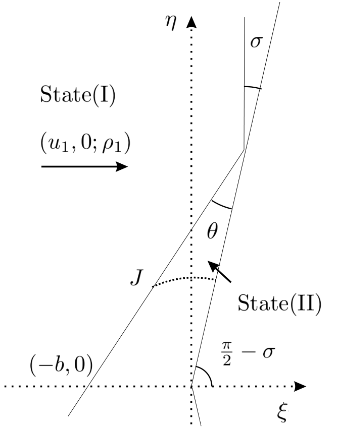
In this subsection, direction of wedge and flow is as illustrated in Figure 10, s.t. Γwedge+\Gamma_{\text{wedge}}^{+} coincides with +η−+\eta-axis. We denote velocity of State(I)(\textup{I}) as (u^1,v^1)=(u1​cos⁡(σ+δ),u1​sin⁡(σ+δ))(\hat{u}_{1},\hat{v}_{1})=(u_{1}\cos(\sigma+\delta),u_{1}\sin(\sigma+\delta)), and velocity of State(II+)(\textup{II}_{+}) as (u2+,v2+)(u_{2}^{+},v_{2}^{+}).

First we compare ϕ\phi and ϕ2+\phi_{2}^{+} on Γshock∪Γsonic+\Gamma_{\text{shock}}\cup\Gamma_{\text{sonic}}^{+}.

Refer to caption
Figure 10: Comparison of ϕ\phi and ϕ2+\phi_{2}^{+}

Assumption (25) implies, Γshock\Gamma_{\text{shock}} is tangent to Γshock+\Gamma_{\text{shock}}^{+} at JJ (here, J≜Γshock¯∩Γsonic+¯J\triangleq\overline{\Gamma_{\text{shock}}}\cap\overline{\Gamma_{\text{sonic}}^{+}}). Here, recall that, Γshock+\Gamma_{\text{shock}}^{+} is the regular reflected shock above ξ\xi-axis. And in section 2.6 we proved that shock is convex. So if we denote that Γshock+\Gamma_{\text{shock}}^{+} lay on a straight line l+l_{+}, then l+l_{+} should be tangent to Γshock\Gamma_{\text{shock}} at JJ, and Γshock\Gamma_{\text{shock}} should stay right to l+l_{+}, as illustrated in Figure 10.

Since on Γshock+\Gamma_{\text{shock}}^{+}, ϕ2+=ϕ1\phi^{+}_{2}=\phi_{1}, and ϕ1,ϕ2+\phi_{1},\phi_{2}^{+} are both linear functions, we have ϕ1=ϕ2+\phi_{1}=\phi_{2}^{+} on l+l_{+}. And since

ϕ1,ξ=u1​cos⁡(σ+δ)>0=u2+=ϕ2,ξ+\phi_{1,\xi}=u_{1}\cos(\sigma+\delta)>0=u_{2}^{+}=\phi_{2,\xi}^{+}

ϕ1≥ϕ2+\phi_{1}\geq\phi_{2}^{+} on Γshock\Gamma_{\text{shock}}. Free boundary condition requires ϕ=ϕ1\phi=\phi_{1} on Γshock\Gamma_{\text{shock}} (26), so ϕ≥ϕ2+\phi\geq\phi_{2}^{+} on Γshock\Gamma_{\text{shock}}.

By assumption ϕ=ϕ2+\phi=\phi_{2}^{+} on Γsonic+\Gamma_{\text{sonic}}^{+} (24). So

ϕ≥ϕ2+​ on Γsonic+∪Γshock\phi\geq\phi_{2}^{+}\text{\ \ on $\Gamma_{\text{sonic}}^{+}\cup\Gamma_{\text{shock}}$} (100)

Then, we compare velocity.

We know u2+=0u_{2}^{+}=0, and analysis in section 2.4 shows u≥0u\geq 0 in Ω\Omega (87), so u≥u2+u\geq u_{2}^{+}.

To vv, we can apply analysis in section 2.3(from (33) to (41)), only replacing ξ\xi-derivative of (33) by η\eta-derivative of (33), to assert that vv cannot achieve minimum or maximum in Ω\Omega or at interior point of Γwedge+\Gamma_{\text{wedge}}^{+} and Γwedge−\Gamma_{\text{wedge}}^{-}.

Then, if vv achieves minimum or maximum at some interior point of Γshock\Gamma_{\text{shock}}, at this point,

vT=0,(here, ​T=(v^1−v,u−u^1))v_{T}=0,(\text{here, }T=(\hat{v}_{1}-v,u-\hat{u}_{1}))

Put this, (59) and (33) together:

(0v^1−vu−u^1R​Hu​(v^1−v)R​Hv​(v^1−v)+R​Hu​(u−u^1)R​Hv​(u−u^1)a112​a12a22)​(uξvξvη)=0\left(\begin{array}[]{ccc}0&\hat{v}_{1}-v&u-\hat{u}_{1}\\ RH_{u}(\hat{v}_{1}-v)&RH_{v}(\hat{v}_{1}-v)+RH_{u}(u-\hat{u}_{1})&RH_{v}(u-\hat{u}_{1})\\ a_{11}&2a_{12}&a_{22}\end{array}\right)\left(\begin{array}[]{c}u_{\xi}\\ v_{\xi}\\ v_{\eta}\end{array}\right)=0

Determinant of this 3×\times3 matrix equals

−R​Hu​(a11​(u−u^1)2−2​a12​(v^1−v)​(u−u^1)+a22​(v^1−v)2)-RH_{u}(a_{11}(u-\hat{u}_{1})^{2}-2a_{12}(\hat{v}_{1}-v)(u-\hat{u}_{1})+a_{22}(\hat{v}_{1}-v)^{2})

In this subsection

R​H=[ρ⁡(u−ξ,v−η)−ρ1​(u^1−ξ,v^1−η)]​(u−u^1,v−v^1), on Γshock,RH=[\rho(u-\xi,v-\eta)-\rho_{1}(\hat{u}_{1}-\xi,\hat{v}_{1}-\eta)](u-\hat{u}_{1},v-\hat{v}_{1}),\text{ on $\Gamma_{\text{shock}}$}, (101)

while ρ\rho is still expressed as (57). Computation shows

R​Hu\displaystyle RH_{u} =ρ2−γγ−1​(ξ−u)​[(u−ξ)​(u−u^1)+(v−η)​(v−v^1)]+ρ⁡(2​u−u^1−ξ)−ρ1​(u^1−ξ)\displaystyle=\frac{\rho^{2-\gamma}}{\gamma-1}(\xi-u)[(u-\xi)(u-\hat{u}_{1})+(v-\eta)(v-\hat{v}_{1})]+\rho(2u-\hat{u}_{1}-\xi)-\rho_{1}(\hat{u}_{1}-\xi) (102)
≤Cp​σ+u1​ρ¯2​(Z2c¯22−1)⏟<−1Cp​(20)+ρ¯2​Z−ρ1​(u1+Z)⏟=0,RH condition for normal shock reflection.\displaystyle\leq C_{p}\sigma+u_{1}\overline{\rho}_{2}\underbrace{\left(\frac{Z^{2}}{\overline{c}_{2}^{2}}-1\right)}_{<-{1\over C_{p}}\text{(\ref{subsonicityofnormallyreflectedshock})}}+\underbrace{\overline{\rho}_{2}Z-\rho_{1}(u_{1}+Z)}_{=0,\text{RH condition for normal shock reflection}}. (103)

So when σ\sigma small enough, if the minimum or maximum of vv is achieved at some point on Γshock\Gamma_{\text{shock}}, then at this point, D2​ϕ=0D^{2}\phi=0, vn=0v_{n}=0. This contradicts with Hopf Lemma, since vv would satisfy a linear elliptic equation without zero order term, similar to (39).

So vv can only achieve its minimum on Γsonic+\Gamma_{\text{sonic}}^{+} and Γsonic−\Gamma_{\text{sonic}}^{-}. In section 1.2, we have shown, in current position, v2−v_{2}^{-} should be ≤0\leq 0, while v2+v_{2}^{+} should be ≥0\geq 0. So v≤v2+v\leq v_{2}^{+} in Ω¯\overline{\Omega}.

Now, we have proved,

  • •

    ϕξ=u≥0=u2+=ϕ2,ξ+,ϕη=v≤v2+=ϕ2,η+\phi_{\xi}=u\geq 0=u_{2}^{+}=\phi_{2,\xi}^{+},\ \phi_{\eta}=v\leq v_{2}^{+}=\phi_{2,\eta}^{+} in Ω¯\overline{\Omega}

  • •

    ϕ≥ϕ2+\phi\geq\phi_{2}^{+} on Γshock∪Γsonic+\Gamma_{\text{shock}}\cup\Gamma_{\text{sonic}}^{+}.

With above estimates, we can tell ϕ≥ϕ2+\phi\geq\phi_{2}^{+} along Γwedge¯\overline{\Gamma_{\text{wedge}}}. And computation gives

ϕ2+<ϕ2−,on Γsonic−,\phi^{+}_{2}<\phi^{-}_{2},\ \text{on $\Gamma_{\text{sonic}}^{-}$},

so ϕ2+<ϕ\phi_{2}^{+}<\phi, on Γsonic−\Gamma_{\text{sonic}}^{-}. So ϕ≥ϕ2+\phi\geq\phi_{2}^{+}, on ∂Ω\partial\Omega.

Since ϕ2+−ϕ\phi_{2}^{+}-\phi satisfies a second order elliptic equation in Ω\Omega, we can conclude

ϕ≥ϕ2+,in ​Ω.\phi\geq\phi_{2}^{+},\ \text{in }\Omega. (104)

2.8 Elliptic Estimates away from the Sonic Circle

In {|η|≤12c¯22−Z2}\{|\eta|\leq{1\over 2}\sqrt{\overline{c}_{2}^{2}-Z^{2}}\} when σ\sigma small enough,

|∇φ|2c2≤12​(c¯22−Z2)+Z2+Cp​σc¯22−Cp​σ=12​(c¯22+Z2)+Cp​σc¯22−Cp​σ<1−1Cp.\frac{|\nabla\varphi|^{2}}{c^{2}}\leq\frac{{1\over 2}(\overline{c}_{2}^{2}-Z^{2})+Z^{2}+C_{p}\sigma}{\overline{c}_{2}^{2}-C_{p}\sigma}=\frac{{1\over 2}(\overline{c}_{2}^{2}+Z^{2})+C_{p}\sigma}{\overline{c}_{2}^{2}-C_{p}\sigma}<1-\frac{1}{C_{p}}.

2.9 Derivative Estimate at Corner of Wedge

Now with Proposition 1, we can control |∇ϕ||\nabla\phi| by CpC_{p}, so according to Lemma A.1 of [4], there exists 0<α<10<\alpha<1, which does not depend on angle of wedge s.t. we can take

ω⁡(r)=Cp​rα,\omega(r)=C_{p}r^{\alpha},

in Lemma 4.3 in [4], and get:

Proposition 3.

Let ϕ\phi be a regular solution in the sense of Definition 1, we can find CpC_{p} and α\alpha (0<α<1)(0<\alpha<1), which do not depend on σ\sigma, s.t.

|∇ϕ|C0≤Cp​rα,in ​Br​(𝒞)∩Ω;\displaystyle|\nabla\phi|_{C^{0}}\leq C_{p}r^{\alpha},\ \text{in }B_{r}(\mathcal{C})\cap\Omega; (105)
|D2​ϕ|C0≤Cp​rα−1,in ​Br​(𝒞)∩Ω.\displaystyle|D^{2}\phi|_{C^{0}}\leq C_{p}r^{\alpha-1},\ \text{in }B_{r}(\mathcal{C})\cap\Omega. (106)

for r<min⁡{Z2,Y2}r<\min\{{Z\over 2},{Y\over 2}\}.

2.10 Hölder Gradient Estimates away from the Sonic Circle and the Corner of the Wedge

In this section we estimate Hölder norm of ∇ϕ\nabla\phi through quasiconformal mapping. Our method is a modification of the method in [15] and Chap 12 of [10].

For q∈Ω¯∩{|η|<Y4}∩{ξ+Z<Z4}q\in\overline{\Omega}\cap\left\{|\eta|<\frac{Y}{4}\right\}\cap\left\{\xi+Z<\frac{Z}{4}\right\}, consider

𝒟⁡(r,q)≜∫Br​(q)∩Ωuξ2+vξ2+uη2+vη2,(0<r<r0≜min⁡{Y4,Z4}).\mathcal{D}(r;q)\triangleq\int_{B_{r}(q)\cap\Omega}u_{\xi}^{2}+v_{\xi}^{2}+u_{\eta}^{2}+v_{\eta}^{2},\ \left(0<r<r_{0}\triangleq\min\left\{\frac{Y}{4},\frac{Z}{4}\right\}\right).
𝒟⁡(r,q)≤\displaystyle\mathcal{D}(r;q)\leq 2​K​∫Br​(q)∩Ω(vξ2−vη​uξ)​(K≜Λλ≤Cp)\displaystyle 2K\int_{B_{r}(q)\cap\Omega}(v_{\xi}^{2}-v_{\eta}u_{\xi})\ (K\triangleq\frac{\Lambda}{\lambda}\leq C_{p})
=\displaystyle= 2K∫Br​(q)∩Ωvξ​Gη−vη​GξGu(in denominator we consider G as a function of u,v,ξ,η,\displaystyle 2K\int_{B_{r}(q)\cap\Omega}\frac{v_{\xi}G_{\eta}-v_{\eta}G_{\xi}}{G_{u}}\ (\text{in denominator we consider $G$}\text{ as a function of $u,v,\xi,\eta$,}
OPENwhile in numerator we consider G as a function of ξ,η)\displaystyle\text{ while in numerator we consider $G$ as a function of $\xi,\eta$})
≤\displaystyle\leq 2​Cp​∫Br​(q)∩Ω∇⋅(vη​G,−vξ​G)​(because vξ2−vη​uξ>0, and Gu≤−1Cp​(94))\displaystyle 2C_{p}\int_{B_{r}(q)\cap\Omega}\nabla\cdot(v_{\eta}G,-v_{\xi}G)\ (\text{because $v_{\xi}^{2}-v_{\eta}u_{\xi}>0$, and $G_{u}\leq-\frac{1}{C_{p}}$}(\ref{negativeupperboundofGu}))
=\displaystyle= 2​Cp​∫∂(Br​(q)∩Ω)G​v𝕥((vη,−vξ)⋅𝕟≜v𝕥)\displaystyle 2C_{p}\int_{\partial(B_{r}(q)\cap\Omega)}Gv_{{\mathbb{t}}}\ \ \left((v_{\eta},-v_{\xi})\cdot\mathbb{n}\triangleq v_{{\mathbb{t}}}\right)
=\displaystyle= 2​Cp​∫(∂Br​(q))∩ΩG​v𝕥(because ​G∣Γshock=0)\displaystyle 2C_{p}\int_{(\partial B_{r}(q))\cap\Omega}Gv_{{\mathbb{t}}}\ \ \left(\text{because }G\mid_{\Gamma_{\text{shock}}}=0\right)
≤\displaystyle\leq Cp​(2​π​r​∫(∂Br​(q))∩Ω|∇v|2)12.\displaystyle C_{p}\left(2\pi r\int_{(\partial B_{r}(q))\cap\Omega}|\nabla v|^{2}\right)^{1\over 2}.

Above means

𝒟​(r,q)2≤Cp​r​d​𝒟​(r,q)d​r⇒dd​r​[1𝒟⁡(r,q)+log⁡rCp]≤0,\mathcal{D}(r;q)^{2}\leq C_{p}r\frac{d\mathcal{D}(r;q)}{dr}\ \Rightarrow\ \frac{d}{dr}\left[\frac{1}{\mathcal{D}(r;q)}+\frac{\log r}{C_{p}}\right]\leq 0,

and after integral we get

𝒟⁡(r,q)≤Cp−log⁡rr0.\mathcal{D}(r;q)\leq\frac{C_{p}}{-\log{r\over r_{0}}}.

Then we estimate growth of 𝒟⁡(r,q)\mathcal{D}(r;q) more precisely with

𝒟⁡(r,q)≤2​Cp​∫(∂Br​(q))∩ΩG​v𝕥.\mathcal{D}(r;q)\leq 2C_{p}\int_{(\partial B_{r}(q))\cap\Omega}Gv_{{\mathbb{t}}}.

1) if (∂Br)∩Γshock≠∅(\partial B_{r})\cap\Gamma_{\text{shock}}\neq\emptyset

𝒟⁡(r,q)≤\displaystyle\mathcal{D}(r;q)\leq Cp​(1μ​∫(∂Br)∩Ω|∇v|2+μ​∫(∂Br)∩ΩG2)\displaystyle C_{p}\left(\frac{1}{\mu}\int_{(\partial B_{r})\cap\Omega}|\nabla v|^{2}+\mu\int_{(\partial B_{r})\cap\Omega}G^{2}\right)
≤\displaystyle\leq Cp​(1μ​∫(∂Br)∩Ω|∇v|2+μ​∫(∂Br)∩Ω|∇G|2​4​π2​r2)(G∣Γshock=0)\displaystyle C_{p}\left(\frac{1}{\mu}\int_{(\partial B_{r})\cap\Omega}|\nabla v|^{2}+\mu\int_{(\partial B_{r})\cap\Omega}|\nabla G|^{2}4\pi^{2}r^{2}\right)\ \ (G\mid_{\Gamma_{\text{shock}}}=0)
=\displaystyle= Cp​r​∫(∂Br)∩Ω|∇u|2+|∇v|2(take ​μ=12​π​r)\displaystyle C_{p}r\int_{(\partial B_{r})\cap\Omega}|\nabla u|^{2}+|\nabla v|^{2}\ \ (\text{take }\mu={1\over 2\pi r})
=\displaystyle= Cp​r​d​𝒟​(r,q)d​r;\displaystyle C_{p}r\frac{d\mathcal{D}(r;q)}{dr};

2) if (∂Br)∩Γshock=∅(\partial B_{r})\cap\Gamma_{\text{shock}}=\emptyset

𝒟⁡(r,q)≤2​Cp​∫(∂Br)∩Ω(G−G¯)​v𝕥,\mathcal{D}(r;q)\leq 2C_{p}\int_{(\partial B_{r})\cap\Omega}(G-\overline{G})v_{{\mathbb{t}}},

again with method above we get

𝒟⁡(r,q)≤Cp​r​d​𝒟​(r,q)d​r.\mathcal{D}(r;q)\leq C_{p}r\frac{d\mathcal{D}(r;q)}{dr}.

Above result implies

𝒟⁡(r,q)≤𝒟⁡(r0/2,q)​(rr0/2)1Cp≤Cp​r1Cp, for ​r<r0/2.\mathcal{D}(r;q)\leq\mathcal{D}(r_{0}/2,q)\left(\frac{r}{r_{0}/2}\right)^{1\over C_{p}}\leq C_{p}r^{1\over C_{p}},\text{ for }r<r_{0}/2.

Then with Lemma 7.16, Lemma 7.18 of [10] and the property that Γshock\Gamma_{\text{shock}} is convex we get:

Proposition 4.

For ϕ\phi, a regular solution in the sense of Definition 1, there exists 0<χ<10<\chi<1 and CpC_{p}, both do not depend on angle of wedge, s.t.

|∇ϕ|χ;ℱ≤Cp,|\nabla\phi|_{\chi;\mathcal{F}}\leq C_{p}, (107)

where we define

ℱ≜(Ω¯∩{|η|<Y4}∩{ξ+Z<Z4}).\mathcal{F}\triangleq\left(\overline{\Omega}\cap\left\{|\eta|<\frac{Y}{4}\right\}\cap\left\{\xi+Z<\frac{Z}{4}\right\}\right).

2.11 C2,χC^{2,\chi} Estimate away from Sonic Circle and Corner of Wedge

Now we consider divergence form equation of GG.

Since ai​j​ϕi​j=0a_{ij}\phi_{ij}=0, given any h∈C0∞​(Ω)h\in C_{0}^{\infty}(\Omega), we have

0=\displaystyle 0= ∫Ω(a11a22​ϕξ​ξ+2​a12a22​ϕξ​η+ϕη​η)​hξ\displaystyle\int_{\Omega}\left({a_{11}\over a_{22}}\phi_{\xi\xi}+{2a_{12}\over a_{22}}\phi_{\xi\eta}+\phi_{\eta\eta}\right)h_{\xi}
=\displaystyle= ∫Ωa11a22​uξ​hξ+2​a12a22​vξ​hξ+uη​hη.\displaystyle\int_{\Omega}{a_{11}\over a_{22}}u_{\xi}h_{\xi}+{2a_{12}\over a_{22}}v_{\xi}h_{\xi}+u_{\eta}h_{\eta}.

Then make use of first two lines of

(uξuηvη)=1D​(a22​Gu−2​a12​Gv−a22​Gva11​Gva22​Gu−a11​Gua11​Gv−2​a12​Gu)​(GξGη),\left(\begin{array}[]{c}u_{\xi}\\ u_{\eta}\\ v_{\eta}\end{array}\right)={1\over D}\left(\begin{array}[]{cc}a_{22}G_{u}-2a_{12}G_{v}&-a_{22}G_{v}\\ a_{11}G_{v}&a_{22}G_{u}\\ -a_{11}G_{u}&a_{11}G_{v}-2a_{12}G_{u}\end{array}\right)\left(\begin{array}[]{c}G_{\xi}\\ G_{\eta}\end{array}\right), (108)

where D=a11​Gv2−2​a12​Gu​Gv+a22​Gu2D=a_{11}G_{v}^{2}-2a_{12}G_{u}G_{v}+a_{22}G_{u}^{2}, we get

∫Ωa11​GuD​Gξ​hξ+a11​GvD​Gξ​hη+−a11​Gv+2​a12​GuD​Gη​hξ+a22​GuD​Gη​hη=0.\int_{\Omega}{a_{11}G_{u}\over D}G_{\xi}h_{\xi}+{a_{11}G_{v}\over D}G_{\xi}h_{\eta}+{-a_{11}G_{v}+2a_{12}G_{u}\over D}G_{\eta}h_{\xi}+{a_{22}G_{u}\over D}G_{\eta}h_{\eta}=0.

With computation we can tell above equation is elliptic in Ω\Omega, when σ\sigma small(Gu≠0G_{u}\neq 0). And we know G∣Γshock=0G\mid_{\Gamma_{\text{shock}}}=0 and |Γshock|1,χ≤Cp|\Gamma_{\text{shock}}|_{1,\chi}\leq C_{p} (107), with Theorem 8.33 of [10], we get

|G|1,χ;ℱ≤Cp,|G|_{1,\chi;\mathcal{F}}\leq C_{p},

where ℱ\mathcal{F} is defined in last subsection.

Since with (108) we can represent D2​ϕD^{2}\phi by derivatives of GG, derivatives of ϕ\phi and ϕ\phi, we can conclude:

Proposition 5.

For ϕ\phi, a regular solution in the sense of Definition 1, and for 0<χ<10<\chi<1, whose existence is argued in last subsection, there exists CpC_{p}, s.t.

|ϕ|2,χ;ℱ≤Cp.|\phi|_{2,\chi;\mathcal{F}}\leq C_{p}. (109)

3 Perturbation of State(II)(\textup{II})

In this section we show that some parameters of State(II±)(\textup{II}_{\pm}) are analytic functions of σ\sigma, and compute the derivative of these parameters w.r.t. σ\sigma and δ\delta.

3.1 Symmetric: Derivatives w.r.t. σ\sigma

In this subsection the position of flow and wedge is as in Figure 3. And we compute derivative of parameters of State(II)(\textup{II}) w.r.t. σ\sigma. If we change σ\sigma to σ+δ\sigma+\delta, results here apply to State(II+)(\textup{II}_{+}); and if we change σ\sigma to σ−δ\sigma-\delta, then results here apply to State​(II−)\text{State}(\textup{II}_{-}), after a reflection.

3.1.1 Parameters of State(II)(\textup{II})

Refer to caption
Figure 11: Parameters of State(II)(\textup{II})

We denote velocity and density of gas in State(II)(\textup{II}) as (u2,v2)(u_{2},v_{2}) and ρ2\rho_{2}; the point where regular reflected shock intersects with sonic circle as JJ; the angle between regular reflected shock and Γwedge\Gamma_{\text{wedge}} as θ\theta; the point where extension line of regular reflected shock intersects with symmetry axis of wedge as (−b,0)(-b,0), as illustrated in Figure 11.

We have the following relations for (v2,ρ2,b,θ)(v_{2},\rho_{2},b,\theta) and σ\sigma.

ρ2γ−1+tan2⁡σ+12​v22+v2​b​tan⁡σ=ρ1γ−1+u122+u1​b\displaystyle\rho_{2}^{\gamma-1}+\frac{\tan^{2}\sigma+1}{2}v_{2}^{2}+v_{2}b\tan\sigma=\rho_{1}^{\gamma-1}+\frac{u_{1}^{2}}{2}+u_{1}b (110)
v2​cos⁡θcos⁡σ=u1​sin⁡(σ+θ)\displaystyle{\centering v_{2}\frac{\cos\theta}{\cos\sigma}=u_{1}\sin(\sigma+\theta)\@add@centering} (111)
(ρ1​(u1+b)−ρ2​(v2​tan⁡σ+b))​(u1−v2​tan⁡σ)\displaystyle(\rho_{1}(u_{1}+b)-\rho_{2}(v_{2}\tan\sigma+b))(u_{1}-v_{2}\tan\sigma)
+ρ2​v22=0\displaystyle+\rho_{2}v_{2}^{2}=0 (112)
X​tan⁡(θ+σ)=tan⁡σ⁡(b+X)\displaystyle X\tan(\theta+\sigma)=\tan\sigma(b+X) (113)

(110) is Bernoulli Law computed at (−b,0)(-b,0), (111) means gas in State(I)(\textup{I}) and State(II)(\textup{II}) have same tangential velocity along regularly reflected shock. (112) is Mass Conservation computed at (−b,0)(-b,0), with (u1−u2,−v2)(u_{1}-u_{2},-v_{2}) taken as normal direction of shock. (113) is a fundamental geometric condition.

Computation shows for σ\sigma small enough, system (110) (111) (112) (113) has a unique solution, which satisfies

|b−Z|≤Cp​σ,|u2|+|v2|≤Cp​σ,|ρ2−ρ¯2|≤Cp​σ,|θ|≤Cp​σ,|b-Z|\leq C_{p}\sigma,|u_{2}|+|v_{2}|\leq C_{p}\sigma,|\rho_{2}-\overline{\rho}_{2}|\leq C_{p}\sigma,|\theta|\leq C_{p}\sigma,

so b,θ,v2,ρ2​ are analytic functions of ​σb,\ \theta,\ v_{2},\ \rho_{2}\text{ are analytic functions of }\sigma. And at σ=0\sigma=0

d​θd​σ=ZX,d​bd​σ=d​ρd​σ=0,d​v2d​σ=u1​(ZX+1).\frac{d\theta}{d\sigma}=\frac{Z}{X},\ \frac{db}{d\sigma}=\frac{d\rho}{d\sigma}=0,\ \frac{dv_{2}}{d\sigma}=u_{1}(\frac{Z}{X}+1).

3.1.2 Coordinates of the Intersection Point

Then we compute the coordinate of JJ where shock intersects with sonic circle, we have:

(ξJ−u2)2+(ηJ−v2)2=c22=(γ−1)​ρ2γ−1,\displaystyle(\xi_{J}-u_{2})^{2}+(\eta_{J}-v_{2})^{2}=c_{2}^{2}=(\gamma-1)\rho_{2}^{\gamma-1}, (114)
(−u1+u2)​ξJ+v2​ηJ+u122−u22+v222+ρ1γ−1−ρ2γ−1=0.\displaystyle(-u_{1}+u_{2})\xi_{J}+v_{2}\eta_{J}+\frac{u_{1}^{2}}{2}-\frac{u_{2}^{2}+v_{2}^{2}}{2}+\rho_{1}^{\gamma-1}-\rho_{2}^{\gamma-1}=0. (115)

From (114)(115), we get, at σ=0\sigma=0,

d​ξJd​σ=(ZX+1)​c¯22−Z2,\displaystyle\frac{d\xi_{J}}{d\sigma}=(\frac{Z}{X}+1)\sqrt{\overline{c}_{2}^{2}-{Z}^{2}}, (116)
d​ηJd​σ=(ZX+1)​(u1+Z).\displaystyle\frac{d\eta_{J}}{d\sigma}=(\frac{Z}{X}+1)(u_{1}+Z). (117)

3.2 Non-symmetric: Derivatives w.r.t. δ\delta

In this subsection we fix the angle between wedge and η\eta-axis as σ0\sigma_{0}, consider the derivatives of (u2+,v2+,ρ2+)(u_{2}^{+},v_{2}^{+},\rho_{2}^{+}) w.r.t. δ\delta for 0≤δ≤σ00\leq\delta\leq\sigma_{0}(here consider u2+,v2+,ρ2+u_{2}^{+},v_{2}^{+},\rho_{2}^{+} as functions of δ\delta).

Refer to caption
Figure 12: Rotation from Symmetric Flow to Symmetric Wedge

With result of last subsection, we get (as illustrated in Figure 12):

(u2+,v2+)=(u2​(σ0+δ),v2​(σ0+δ))​(cos⁡δsin⁡δ−sin⁡δcos⁡δ)(u_{2}^{+},v_{2}^{+})=(u_{2}(\sigma_{0}+\delta),v_{2}(\sigma_{0}+\delta))\left(\begin{array}[]{cc}\cos\delta&\sin\delta\\ -\sin\delta&\cos\delta\end{array}\right)
⇒d​u2+d​δ=O⁡(σ0),d​v2+d​δ=u1​(ZX+1)+O⁡(σ0)\Rightarrow\frac{du_{2}^{+}}{d\delta}=O(\sigma_{0}),\ \ \frac{dv_{2}^{+}}{d\delta}=u_{1}({Z\over X}+1)+O(\sigma_{0})
(ξJ+,ηJ+)=(ξJ​(σ0+δ),ηJ​(σ0+δ))​(cos⁡δsin⁡δ−sin⁡δcos⁡δ)(\xi_{J}^{+},\eta_{J}^{+})=(\xi_{J}(\sigma_{0}+\delta),\eta_{J}(\sigma_{0}+\delta))\left(\begin{array}[]{cc}\cos\delta&\sin\delta\\ -\sin\delta&\cos\delta\end{array}\right)
⇒d​ξJ+d​δ=ZX​c¯22−Z2+O⁡(σ0),d​ηJ+d​δ=u1​(ZX+1)+Z2X+O⁡(σ0)\Rightarrow\frac{d\xi_{J}^{+}}{d\delta}=\frac{Z}{X}\sqrt{\overline{c}_{2}^{2}-Z^{2}}+O(\sigma_{0}),\ \ \frac{d\eta_{J}^{+}}{d\delta}=u_{1}(\frac{Z}{X}+1)+\frac{Z^{2}}{X}+O(\sigma_{0})

Then we analyze motion of Sonic Circle.

Any point pp on Γsonic+\Gamma_{\text{sonic}}^{+} takes the following form:

p=c2+(cosα,sinα)+(u2+,v2+)(π2−σ0<α<π2−σ0+α0,α0=π2−12arccosZc2)p=c_{2}^{+}(\cos\alpha,\sin\alpha)+(u_{2}^{+},v_{2}^{+})\ ({\pi\over 2}-\sigma_{0}<\alpha<{\pi\over 2}-\sigma_{0}+\alpha_{0},\ \alpha_{0}={\pi\over 2}-{1\over 2}\arccos\frac{Z}{c_{2}})

and

d​pd​δ=(O⁡(σ0),u1​(ZX+1)+O⁡(σ0)).\frac{dp}{d\delta}=(O(\sigma_{0}),u_{1}(\frac{Z}{X}+1)+O(\sigma_{0})).

So if we rotate upstream flow counterclockwise(δ>0\delta>0), and σ0\sigma_{0} small enough s.t.

O⁡(σ0)u1​(ZX+1)+O⁡(σ0)≤c¯22−Z22​Z,\frac{O(\sigma_{0})}{u_{1}(\frac{Z}{X}+1)+O(\sigma_{0})}\leq\frac{\sqrt{\overline{c}_{2}^{2}-Z^{2}}}{2Z},

then every point on Γsonic+\Gamma_{\text{sonic}}^{+} moves up. If we rotate upstream flow clockwise(corresponds to δ<0\delta<0), then sonic circle moves down.

3.3 Comparison of State(II+)(\textup{II}_{+}) and State(II−)(\textup{II}_{-})

Now with computation above we compare physical quantity and geometric structure of State(II+)(\textup{II}_{+}) and State​(II−)\text{State}(\textup{II}_{-}).

3.3.1 Comparison of Geometric Structures

Figure 13: Relative Positions of Γsonic+,Γshock,Γsonic−~\Gamma_{\text{sonic}}^{+},\ \Gamma_{\text{shock}},\ \widetilde{\Gamma_{\text{sonic}}^{-}}

We compare State(II+)(\textup{II}_{+}) and State(II−)(\textup{II}_{-}), by reflecting State(II−)(\textup{II}_{-}) across symmetry axis of wedge. And for any point pp (or set AA), p~\tilde{p} (and A~\tilde{A}) denotes the reflection of pp (and AA) into symmetry axis of wedge. So J−~,Γsonic−~,Γshock~\widetilde{J^{-}},\ \widetilde{\Gamma_{\text{sonic}}^{-}},\ \widetilde{\Gamma_{\text{shock}}} are the reflection of J−,Γsonic−,ΓshockJ^{-},\ \Gamma_{\text{sonic}}^{-},\ \Gamma_{\text{shock}}, and if we consider them as set valued function of δ\delta, then

J−​(δ)~=J+​(−δ),Γsonic−​(δ)~=Γsonic+​(−δ).\widetilde{J^{-}(\delta)}=J^{+}(-\delta),\ \widetilde{\Gamma_{\text{sonic}}^{-}(\delta)}=\Gamma_{\text{sonic}}^{+}(-\delta).

With computation result we have, we know when σ0\sigma_{0} small enough and δ>0\delta>0, Γsonic+\Gamma_{\text{sonic}}^{+} should stay above Γsonic−~\widetilde{\Gamma_{\text{sonic}}^{-}}, and Γshock−~\widetilde{\Gamma_{\text{shock}}^{-}} should not intersect with Γsonic+\Gamma_{\text{sonic}}^{+} and Γshock\Gamma_{\text{shock}}. So relative position of Γsonic+,Γshock,Γsonic−~,Γshock−~\Gamma_{\text{sonic}}^{+},\ \Gamma_{\text{shock}},\ \widetilde{\Gamma_{\text{sonic}}^{-}},\ \widetilde{\Gamma_{\text{shock}}^{-}} should be as illustrated in Figure 13.

3.3.2 Comparison of ϕ2+\phi_{2}^{+} and ϕ2−\phi_{2}^{-}

With (22),

ϕ2+=−ρ2+γ−1+ρ0γ−1+u2+​ξ+v2+​η−u2+2+v2+22,\phi_{2}^{+}=-{\rho_{2}^{+}}^{\gamma-1}+{\rho_{0}^{\gamma-1}}+u_{2}^{+}\xi+v^{+}_{2}\eta-\frac{{u_{2}^{+}}^{2}+{v_{2}^{+}}^{2}}{2},
ϕ2−=−ρ2−γ−1+ρ0γ−1+u2−​ξ+v2−​η−u2−2+v2−22,\phi_{2}^{-}=-{\rho_{2}^{-}}^{\gamma-1}+{\rho_{0}^{\gamma-1}}+u_{2}^{-}\xi+v^{-}_{2}\eta-\frac{{u_{2}^{-}}^{2}+{v_{2}^{-}}^{2}}{2},

so on {η=0}\{\eta=0\}, which is the symmetry axis of wedge,

|ϕ2+−ϕ2−|≤Cp​σ0​δ.|\phi_{2}^{+}-\phi_{2}^{-}|\leq C_{p}\sigma_{0}\delta.

And v2+−v2−>1Cp​δv_{2}^{+}-v_{2}^{-}>\frac{1}{C_{p}}\delta, so when σ0\sigma_{0} small enough

ϕ2+>ϕ2−~+δCp,on {η>c¯22−Z22},\phi_{2}^{+}>\widetilde{\phi_{2}^{-}}+{\delta\over C_{p}},\ \ \text{on }\{\eta>{\sqrt{\overline{c}_{2}^{2}-Z^{2}}\over 2}\}, (118)

where, ϕ2−~\widetilde{\phi_{2}^{-}} is the reflection of ϕ2−\phi_{2}^{-},

ϕ2−~​(ξ,η)=ϕ2−​(ξ,−η).\widetilde{\phi_{2}^{-}}(\xi,\eta)=\phi_{2}^{-}(\xi,-\eta).

3.4 Stronger Comparison

In section 5 we need a more precise estimate, we need to shift J±,Γsonic±J^{\pm},\ \Gamma_{\text{sonic}}^{\pm} by (∓u1sinδtanσ0,−u1sinδ)(\mp u_{1}\sin\delta\tan\sigma_{0},-u_{1}\sin\delta). We denote

J^±=J±−(±u1sinδtanσ0,u1sinδ),\hat{J}^{\pm}=J^{\pm}-(\pm u_{1}\sin\delta\tan\sigma_{0},u_{1}\sin\delta),
Γ^sonic±=Γsonic±−(±u1sinδtanσ0,u1sinδ).\hat{\Gamma}_{\text{sonic}}^{\pm}=\Gamma_{\text{sonic}}^{\pm}-(\pm u_{1}\sin\delta\tan\sigma_{0},u_{1}\sin\delta).

With previous results, in section 3.2, we get

d​J^+d​δ=ZX​(c¯22−Z2+O⁡(σ0),u1+Z+O⁡(σ0)).\frac{d\hat{J}^{+}}{d\delta}=\frac{Z}{X}(\sqrt{\overline{c}_{2}^{2}-Z^{2}}+O(\sigma_{0}),u_{1}+Z+O(\sigma_{0})).

And points qq on Γ^sonic+{\hat{\Gamma}}_{\text{sonic}}^{+} can be parametrized by

q=c2+(cosα,sinα)+(u2+,v2+)−(u1sinδtanσ0,u1sinδ),q=c_{2}^{+}(\cos\alpha,\sin\alpha)+(u_{2}^{+},v_{2}^{+})-(u_{1}\sin\delta\tan\sigma_{0},u_{1}\sin\delta),

for

π2−σ0<α<π2−σ0+α0,α0=π2−12​arccos⁡Zc¯2,{\pi\over 2}-\sigma_{0}<\alpha<{\pi\over 2}-\sigma_{0}+\alpha_{0},\ \ \ \alpha_{0}={\pi\over 2}-{1\over 2}\arccos\frac{Z}{\overline{c}_{2}},

then,

d​qd​δ=(O⁡(σ0),u1​ZX+O⁡(σ0)).\frac{dq}{d\delta}=(O(\sigma_{0}),u_{1}\frac{Z}{X}+O(\sigma_{0})).

And this shift does not change tangential direction of shock, so after this shift, relative position of Γsonic+,Γshock,Γsonic−~\Gamma_{\text{sonic}}^{+},\ \Gamma_{\text{shock}},\ \widetilde{\Gamma_{\text{sonic}}^{-}} remains, as illustrated in Figure 13.

4 Symmetric Estimates

Figure 14: Reflective Comparison

In this part we show that, given a regular solution to the potential flow equation, with velocity of upstream flow being (u1​cos⁡δ,u1​sin⁡δ)(u_{1}\cos\delta,u_{1}\sin\delta), the solution should be “δ\delta-symmetric” w.r.t. η\eta. Before more precisely present the result of this section, we introduce the following notations:

Notation.

In this section we define:

ΓS​A\Gamma_{SA}=Symmetry Axis of wedge.

For any function ff, f~​(ξ,η)=f​(ξ,−η)\tilde{f}(\xi,\eta)=f(\xi,-\eta). And for any set 𝒮\mathcal{S}, 𝒮~\tilde{\mathcal{S}} is the reflection of 𝒮\mathcal{S} along ΓS​A\Gamma_{SA},

Ωc=Ω∩Ω~\Omega_{c}=\Omega\cap\tilde{\Omega} (means “common domain”).

And when σ\sigma is small, based on estimate of section 2.3, ∇ϕ\nabla\phi is small, so it’s clear that we can divide ∂Ω\partial\Omega into“free boundary part”,“sonic circle part” and“upper(or lower) sonic circle part”. We denote them by ∂FΩ\partial_{F}\Omega, ∂SΩ\partial_{S}\Omega and ∂S+Ω⁡(or ​∂S−Ω)\partial_{S}^{+}\Omega(\text{or }\partial_{S}^{-}\Omega) respectively. Similarly ∂FΩc\partial_{F}\Omega_{c} means the free boundary part of the boundary of “common domain”.

And the part of Ω\Ω~\Omega\backslash\tilde{\Omega} above ∂S+Ω~\partial_{S}^{+}\tilde{\Omega} is denoted by H+H^{+}, similarly the part of Ω~\Ω\tilde{\Omega}\backslash\Omega below ∂S−Ω\partial_{S}^{-}\Omega is denoted by H−H^{-}.

On ∂Ω\partial\Omega and ∂Ω~\partial\tilde{\Omega}, 𝕟\mathbb{n} is unit outer normal direction of Ω\Omega and Ω~\tilde{\Omega}.

And in Ω∪Ω~\Omega\cup\widetilde{\Omega} define:

h={ϕ−ϕ~, in ​Ωcϕ1−ϕ~, in ​(Ω~\Ω)\H−ϕ−ϕ1~, in ​(Ω\Ω~)\H+ϕ−ϕ2−~, in ​H+ϕ2−−ϕ~, in ​H−h=\left\{\begin{array}[]{cc}\phi-\tilde{\phi},&\text{ in }\Omega_{c}\\ \phi_{1}-\tilde{\phi},&\text{ in }(\tilde{\Omega}\backslash\Omega)\backslash H^{-}\\ \phi-\widetilde{\phi_{1}},&\text{ in }(\Omega\backslash\tilde{\Omega})\backslash H^{+}\\ \phi-\widetilde{\phi_{2}^{-}},&\text{ in }H^{+}\\ \phi_{2}^{-}-\tilde{\phi},&\text{ in }H^{-}\end{array}\right.
h+=max⁡{h,0},h^{+}=\max\{h,0\},
w=(h+)2.w=(h^{+})^{2}.

In this section we prove:

Section 4.1

∫Ωc|ϕ−ϕ~|3≤Cp⋅δ3\int_{\Omega_{c}}|\phi-\tilde{\phi}|^{3}\leq C_{p}\cdot\delta^{3}

Section 4.2.1

|ϕ−ϕ~|≤Cp​δ|\phi-\tilde{\phi}|\leq C_{p}\delta, in BZ8​(𝒞)B_{Z\over 8}(\mathcal{C})

Section 4.2.2

|ϕη|≤Cp​δ​rα2−1,along ΓS​A near corner of wedge \ |\phi_{\eta}|\leq C_{p}\delta r^{{\alpha\over 2}-1},\ \ \ \text{along $\Gamma_{SA}$ near corner of wedge }

Section 4.3.1

|ϕ−ϕ~|≤Cp​δ​, in a neighborhood of Γshock∩ΓS​A\ |\phi-\tilde{\phi}|\leq C_{p}\delta\text{,\ \ \ in a neighborhood of $\Gamma_{\text{shock}}\cap\Gamma_{SA}$}

Section 4.3.2

|ϕη|≤Cp​δ,along ΓS​A near Γshock|\phi_{\eta}|\leq C_{p}\delta,\ \ \ \ \text{along $\Gamma_{SA}$ near $\Gamma_{\text{shock}}$}

4.1 Integral Symmetric Estimates

Now we consider the following integral:

I\displaystyle I =∫Ωcρ∇⋅φ∇w−ρ~∇φ~⋅∇w−2ρw+2ρ~w\displaystyle=\int_{\Omega_{c}}\rho\nabla\cdot\varphi\nabla w-\tilde{\rho}\nabla\tilde{\varphi}\cdot\nabla w-2\rho w+2\tilde{\rho}w
=∫Ωc∇⋅[ρ∇φw−ρ~∇φ~w](we used equation ∇⋅[ρ∇φ]+2ρ=0).\displaystyle=\int_{\Omega_{c}}\nabla\cdot[\rho\nabla\varphi w-\tilde{\rho}\nabla\tilde{\varphi}w]\ (\text{we used equation }\nabla\cdot[\rho\nabla\varphi]+2\rho=0).

Since we know Γshock\Gamma_{\text{shock}} is the graph of a C1C^{1} function of η\eta (66), ∂Ωc\partial\Omega_{c} should be Lipschitz, so 𝕟\mathbb{n} is defined a.e.. With Green formula generalized to domain with Lipschitz boundary (Lemma 14.4 of [21]), we can reduce II to boundary integral,

I\displaystyle I =∫∂Ωcρ​D𝕟​φ​w−ρ~​D𝕟​φ~​w\displaystyle=\int_{\partial\Omega_{c}}\rho D_{\mathbb{n}}\varphi w-\tilde{\rho}D_{\mathbb{n}}\tilde{\varphi}w
=∫∂SΩcρ​D𝕟​φ​w−ρ~​D𝕟​φ~​w+∫∂FΩcρ​D𝕟​φ​w−ρ~​D𝕟​φ~​w≜IS+IF.\displaystyle=\int_{\partial_{S}\Omega_{c}}\rho D_{\mathbb{n}}\varphi w-\tilde{\rho}D_{\mathbb{n}}\tilde{\varphi}w+\int_{\partial_{F}\Omega_{c}}\rho D_{\mathbb{n}}\varphi w-\tilde{\rho}D_{\mathbb{n}}\tilde{\varphi}w\triangleq I_{S}+I_{F}.

Here we don’t need to consider boundary integral on boundary of wedge, because on boundary of wedge D𝕟​φ=0D_{\mathbb{n}}\varphi=0.

Then we estimate integral on ∂SΩc\partial_{S}\Omega_{c} and ∂FΩc\partial_{F}\Omega_{c} separately, first we estimate integral on sonic circle.

IS=\displaystyle I_{S}= ∫∂SΩcρ​D𝕟​φ​w−ρ~​D𝕟​φ~​w\displaystyle\int_{\partial_{S}\Omega_{c}}\rho D_{\mathbb{n}}\varphi w-\tilde{\rho}D_{\mathbb{n}}\tilde{\varphi}w
=\displaystyle= ∫∂S+Ωcρ​D𝕟​φ​w−ρ~​D𝕟​φ~​w+∫∂S−Ωcρ​D𝕟​φ​w−ρ~​D𝕟​φ~​w⏟=0​(w=0,(118),(104)).\displaystyle\int_{\partial_{S}^{+}\Omega_{c}}\rho D_{\mathbb{n}}\varphi w-\tilde{\rho}D_{\mathbb{n}}\tilde{\varphi}w+\underbrace{\int_{\partial_{S}^{-}\Omega_{c}}\rho D_{\mathbb{n}}\varphi w-\tilde{\rho}D_{\mathbb{n}}\tilde{\varphi}w}_{=0(w=0,(\ref{antisymmetricestimateofphi2}),(\ref{comparisonofphiandphitwoplus}))}.

By symmetry, (118) of section 3.3.2 implies, on ∂S−Ωc\partial_{S}^{-}\Omega_{c} ϕ2−<ϕ2+~\phi_{2}^{-}<\widetilde{\phi^{+}_{2}}; and ϕ2+~≤ϕ~\widetilde{\phi^{+}_{2}}\leq\tilde{\phi} (104), so ϕ=ϕ2−<ϕ2+~≤ϕ~\phi=\phi_{2}^{-}<\widetilde{\phi^{+}_{2}}\leq\tilde{\phi}, w=0w=0. And similar argument shows h>0h>0 in H+H^{+}, so

IS=\displaystyle I_{S}= ∫∂S+ΩcρD𝕟φw−ρ2−~D𝕟φ2−~w(because ϕ=ϕ2−,∇ϕ=∇ϕ2− on Γsonic−)\displaystyle\int_{\partial_{S}^{+}\Omega_{c}}\rho D_{\mathbb{n}}\varphi w-\widetilde{\rho_{2}^{-}}D_{\mathbb{n}}\widetilde{\varphi_{2}^{-}}w\ (\text{because }\ \phi=\phi_{2}^{-},\ \nabla\phi=\nabla\phi_{2}^{-}\text{ on }\Gamma_{\text{sonic}}^{-})
=\displaystyle= ∫H+−∇⋅[(ρ∇φ−ρ2−~∇φ2−~)h2]\displaystyle\int_{H^{+}}-\nabla\cdot[(\rho\nabla\varphi-\widetilde{\rho_{2}^{-}}\nabla\widetilde{\varphi_{2}^{-}})h^{2}]
+∫∂S+Ω(ρ​D𝕟​φ−ρ2−~​D𝕟​φ2−~)​h2⏟≤Cp​δ3​(ρ=ρ2+,∇φ=∇φ2+)+∫(∂FΩ)∩H+¯(ρ​D𝕟​φ−ρ2−~​D𝕟​φ2−~)​h2⏟≤Cp​δ3​(h≤Cp​δ, and length of curve≤Cp​δ)\displaystyle+\int_{\partial_{S}^{+}\Omega}\underbrace{(\rho D_{\mathbb{n}}\varphi-\widetilde{\rho_{2}^{-}}D_{\mathbb{n}}\widetilde{\varphi_{2}^{-}})h^{2}}_{\leq C_{p}\delta^{3}(\rho=\rho_{2}^{+},\nabla\varphi=\nabla\varphi_{2}^{+})}+\underbrace{\int_{(\partial_{F}\Omega)\cap\overline{H^{+}}}(\rho D_{\mathbb{n}}\varphi-\widetilde{\rho_{2}^{-}}D_{\mathbb{n}}\widetilde{\varphi_{2}^{-}})h^{2}}_{\leq C_{p}\delta^{3}\ (h\leq C_{p}\delta,\text{ and length of curve}\leq C_{p}\delta)}
≤\displaystyle\leq ∫H+−2h[(ρ∇φ−ρ2−~∇φ2−~)⋅∇h−(ρ−ρ2−~)h]+Cpδ3\displaystyle\int_{H^{+}}-2h[(\rho\nabla\varphi-\widetilde{\rho_{2}^{-}}\nabla\widetilde{\varphi_{2}^{-}})\cdot\nabla h-(\rho-\widetilde{\rho_{2}^{-}})h]+C_{p}\delta^{3}
≤\displaystyle\leq ∫H+−2h[(ρ∇φ−ρ2+∇φ2+)⋅∇g−(ρ−ρ2+)g]+Cpδ3(here g≜ϕ−ϕ2+).\displaystyle\int_{H^{+}}-2h[(\rho\nabla\varphi-\rho_{2}^{+}\nabla\varphi_{2}^{+})\cdot\nabla g-(\rho-\rho_{2}^{+})g]+C_{p}\delta^{3}\ (\text{here }g\triangleq\phi-\phi_{2}^{+}).

Last inequality follows from

  • •

    width of H+≤Cp​δ,h≤Cp​σH^{+}\leq C_{p}\delta,\ h\leq C_{p}\sigma;

  • •

    |ϕ2+−ϕ2−~|≤Cp​δ,|∇ϕ2+−∇ϕ2−~|≤Cp​δ,|ρ2+−ρ2−~|≤Cp​δ|\phi_{2}^{+}-\widetilde{\phi_{2}^{-}}|\leq C_{p}\delta,|\nabla\phi_{2}^{+}-\nabla\widetilde{\phi_{2}^{-}}|\leq C_{p}\delta,|\rho_{2}^{+}-\widetilde{\rho_{2}^{-}}|\leq C_{p}\delta.

Then as in [7], define

f(t)=φ2++t​g,r(t)=(ρ0γ−1−f(t)−|∇f(t)|22)1γ−1.{f^{(t)}}=\varphi_{2}^{+}+tg,\ {r^{(t)}}=\left(\rho_{0}^{\gamma-1}-{f^{(t)}}-\frac{{|\nabla{f^{(t)}}|}^{2}}{2}\right)^{1\over\gamma-1}.
(ρ∇φ−ρ2+∇φ2+)⋅∇g−(ρ−ρ2+)g\displaystyle(\rho\nabla\varphi-\rho_{2}^{+}\nabla\varphi_{2}^{+})\cdot\nabla g-(\rho-\rho_{2}^{+})g
=\displaystyle= ∫01dd​t[r(t)∇f(t)]⋅∇g−(dd​tr(t))g\displaystyle\int_{0}^{1}\frac{d}{dt}[{r^{(t)}}\nabla{f^{(t)}}]\cdot\nabla g-(\frac{d}{dt}{r^{(t)}})g
=\displaystyle= ∫01r(t)|∇g|2+r(t)2−γ​(−g−∇f(t)⋅∇g)γ−1∇f(t)⋅∇g+∫01r(t)2−γγ−1(g+∇f(t)⋅∇g)g\displaystyle\int_{0}^{1}{r^{(t)}}|\nabla g|^{2}+\frac{{r^{(t)}}^{2-\gamma}(-g-\nabla{f^{(t)}}\cdot\nabla g)}{\gamma-1}\nabla{f^{(t)}}\cdot\nabla g+\int_{0}^{1}\frac{{r^{(t)}}^{2-\gamma}}{\gamma-1}(g+\nabla{f^{(t)}}\cdot\nabla g)g
=\displaystyle= ∫01[r(t)​δi​j−r(t)2−γγ−1​f(t)i​f(t)j]​gi​gj+∫01r(t)2−γγ−1​g2≥0.\displaystyle\int_{0}^{1}[{r^{(t)}}\delta_{ij}-\frac{{r^{(t)}}^{2-\gamma}}{\gamma-1}{f^{(t)}}_{i}{f^{(t)}}_{j}]g_{i}g_{j}+\int_{0}^{1}\frac{{r^{(t)}}^{2-\gamma}}{\gamma-1}g^{2}\geq 0.

In inequality above,

(r(t)​δi​j−r(t)2−γγ−1​f(t)i​f(t)j)>0,(as matrix).\left({r^{(t)}}\delta_{ij}-\frac{{r^{(t)}}^{2-\gamma}}{\gamma-1}{f^{(t)}}_{i}{f^{(t)}}_{j}\right)>0,\ \ (\text{as matrix}).

This follows from the fact that,

(δi​j−r(0)1−γγ−1​f(0)i​f(0)j)=(δi​j−φ2,i+​φ2,j+(γ−1)​ρ2+γ−1)>0,\displaystyle\left(\delta_{ij}-\frac{{r^{(0)}}^{1-\gamma}}{\gamma-1}{f^{(0)}}_{i}{f^{(0)}}_{j}\right)=\left(\delta_{ij}-\frac{\varphi^{+}_{2,i}\varphi^{+}_{2,j}}{(\gamma-1){\rho_{2}^{+}}^{\gamma-1}}\right)>0,
(δi​j−r(1)1−γγ−1​f(1)i​f(1)j)=(δi​j−φi​φj(γ−1)​ργ−1)>0,\displaystyle\left(\delta_{ij}-\frac{{r^{(1)}}^{1-\gamma}}{\gamma-1}{f^{(1)}}_{i}{f^{(1)}}_{j}\right)=\left(\delta_{ij}-\frac{\varphi_{i}\varphi_{j}}{(\gamma-1){\rho}^{\gamma-1}}\right)>0,

because H+H^{+} is the subsonic region for both φ\varphi and φ2+\varphi_{2}^{+}, and

−(γ−1)​r(t)γ−1+|∇f(t)|2​ is a convex function of ​t.\displaystyle-(\gamma-1){r^{(t)}}^{\gamma-1}+|\nabla{f^{(t)}}|^{2}\text{ is a convex function of }t.

More detail and explanation of this method is contained in [7]. So

∫∂SΩcρ​D𝕟​φ​w−ρ~​D𝕟​φ~​w≤Cp​δ3.\int_{\partial_{S}\Omega_{c}}\rho D_{\mathbb{n}}\varphi w-\tilde{\rho}D_{\mathbb{n}}\tilde{\varphi}w\leq C_{p}\delta^{3}.

Then we estimate integral on free boundary

IF=\displaystyle I_{F}= ∫∂FΩc(ρ∇φw−ρ~∇φ~w)⋅𝕟\displaystyle\int_{\partial_{F}\Omega_{c}}(\rho\nabla\varphi w-\tilde{\rho}\nabla\tilde{\varphi}w)\cdot\mathbb{n}
=\displaystyle= ∫(∂FΩ)∩Ω~(ρ1∇φ1w−ρ~∇φ~w)⋅𝕟+∫(∂FΩ~)∩Ω(ρ∇φw−ρ1∇φ1~w)⋅𝕟\displaystyle\int_{(\partial_{F}\Omega)\cap\tilde{\Omega}}(\rho_{1}\nabla\varphi_{1}w-\tilde{\rho}\nabla\tilde{\varphi}w)\cdot\mathbb{n}+\int_{(\partial_{F}\tilde{\Omega})\cap\Omega}(\rho\nabla\varphi w-{\rho_{1}}\nabla\widetilde{\varphi_{1}}w)\cdot\mathbb{n}
+∫(∂FΩ)∩(∂FΩ~)(ρ∇φw−ρ~∇φ~w)⋅𝕟.\displaystyle+\int_{(\partial_{F}\Omega)\cap{(\partial_{F}\tilde{\Omega})}}(\rho\nabla\varphi w-\tilde{\rho}\nabla\tilde{\varphi}w)\cdot\mathbb{n}. (119)

In (119), the third term can be a little complex, since (∂FΩ)∩(∂FΩ~)(\partial_{F}\Omega)\cap{(\partial_{F}\tilde{\Omega})} may be a set of isolated points, but with positive 1-dim Hausdorff measure. And on (∂FΩ)∩(∂FΩ~)(\partial_{F}\Omega)\cap{(\partial_{F}\tilde{\Omega})}, 𝕟\mathbb{n} is not trivially related to normal of Ω\Omega and Ω~\tilde{\Omega}.

Since we know Γshock\Gamma_{\text{shock}} is the graph of a C1C^{1} function of η\eta (66), so let Γshock\Gamma_{\text{shock}} be the graph of f1f_{1}, and Γ~shock=∂FΩ~\widetilde{\Gamma}_{\text{shock}}=\partial_{F}\tilde{\Omega} be the graph of f2f_{2}, with f1f_{1} and f2f_{2} both being C1C^{1} functions of η\eta. And let P​r​o​jProj be the projection from ℝ2{\mathbb{R}}^{2} to ℝ={η}{\mathbb{R}}=\{\eta\}. So on ℱ≜P​r​o​j​(∂FΩc)⊂ℝ\mathcal{F}\triangleq Proj(\partial_{F}\Omega_{c})\subset\mathbb{R}, f1f_{1} and f2f_{2} are both defined, and actually, in the following, we only need to consider f1f_{1} and f2f_{2} as functions defined on ℱ\mathcal{F} , since Γshock∩Γshock~⊂∂FΩc\Gamma_{\text{shock}}\cap\widetilde{\Gamma_{\text{shock}}}\subset\partial_{F}\Omega_{c}.

So Proj(Γshock∩Γshock~)={f1=f2}Proj(\Gamma_{\text{shock}}\cap\widetilde{\Gamma_{\text{shock}}})=\{f_{1}=f_{2}\} is a measurable set in ℝ\mathbb{R}. And since we have an estimate of f1′f_{1}^{\prime} and f2′f_{2}^{\prime} (|u|≤Cp​σ|u|\leq C_{p}\sigma (78), |v|≤Cp​σ|v|\leq C_{p}\sigma (68)), the 1-dim Hausdorff measure on Γshock∩Γshock~\Gamma_{\text{shock}}\cap\widetilde{\Gamma_{\text{shock}}} is equivalent to 1-dim Lebesgue measure on {f1=f2}\{f_{1}=f_{2}\}.

On {f1=f2}\{f_{1}=f_{2}\}, except a set of measure zero, any point is a Lebesgue point. For a Lebesgue point of {f1=f2}\{f_{1}=f_{2}\}, say aa, we can find a sequence {ai}i=0∞\{a_{i}\}_{i=0}^{\infty}, s.t.

limi→∞ai=a⁡(ai≠a),and f1​(ai)=f2​(ai).\lim_{i\rightarrow\infty}a_{i}=a\ (a_{i}\neq a),\ \ \text{and }\ \ f_{1}(a_{i})=f_{2}(a_{i}). (120)

Since we assumed f1f_{1} and f2f_{2} are C1C^{1} functions of η\eta,

f1′​(a)=limi→∞f1​(ai)−f1​(a)ai−a=limi→∞f2​(ai)−f2​(a)ai−a=f2′​(a),f_{1}^{\prime}(a)=\lim_{i\rightarrow\infty}\frac{f_{1}(a_{i})-f_{1}(a)}{a_{i}-a}=\lim_{i\rightarrow\infty}\frac{f_{2}(a_{i})-f_{2}(a)}{a_{i}-a}=f_{2}^{\prime}(a), (121)

f1′=f2′f_{1}^{\prime}=f_{2}^{\prime} a.e. on {f1=f2}\{f_{1}=f_{2}\}. So, on Γshock∩Γshock~\Gamma_{\text{shock}}\cap\widetilde{\Gamma_{\text{shock}}}, Γshock\Gamma_{\text{shock}} and Γshock~\widetilde{\Gamma_{\text{shock}}} have same normal directions a.e., w.r.t. the 1-dim Hausdorff measure on Γshock∩Γshock~\Gamma_{\text{shock}}\cap\widetilde{\Gamma_{\text{shock}}}. So,

(ρ∇φ−ρ~∇φ~)⋅𝕟=(ρ1∇φ1−ρ1∇φ1~)⋅𝕟≤Cpδa.e. on Γshock∩Γshock~.(\rho\nabla\varphi-\tilde{\rho}\nabla\tilde{\varphi})\cdot{\mathbb{n}}=(\rho_{1}\nabla\varphi_{1}-{\rho_{1}}\nabla\widetilde{\varphi_{1}})\cdot{\mathbb{n}}\leq C_{p}\delta\ \ \text{a.e. on $\Gamma_{\text{shock}}\cap\widetilde{\Gamma_{\text{shock}}}$}. (122)

And on Γshock∩Γshock~\Gamma_{\text{shock}}\cap\widetilde{\Gamma_{\text{shock}}}, w≤|h|2=|φ1~−φ1|2≤Cp​δ2w\leq|h|^{2}=|\widetilde{\varphi_{1}}-\varphi_{1}|^{2}\leq C_{p}\delta^{2}. Combining this with (122) gives

∫(∂FΩ)∩(∂FΩ~)(ρ∇φw−ρ~∇φ~w)⋅𝕟≤Cpδ3.\int_{(\partial_{F}\Omega)\cap{(\partial_{F}\tilde{\Omega})}}(\rho\nabla\varphi w-\tilde{\rho}\nabla\tilde{\varphi}w)\cdot\mathbb{n}\leq C_{p}\delta^{3}.

By plugging this into (119), we can reduce IFI_{F} to

IF≤∫(∂FΩ)∩Ω~(ρ1∇φ1w−ρ~∇φ~w)⋅𝕟+∫(∂FΩ~)∩Ω(ρ∇φw−ρ1∇φ1~w)⋅𝕟+Cpδ3.I_{F}\leq\int_{(\partial_{F}\Omega)\cap\tilde{\Omega}}(\rho_{1}\nabla\varphi_{1}w-\tilde{\rho}\nabla\tilde{\varphi}w)\cdot\mathbb{n}+\int_{(\partial_{F}\tilde{\Omega})\cap\Omega}(\rho\nabla\varphi w-{\rho_{1}}\nabla\widetilde{\varphi_{1}}w)\cdot\mathbb{n}+C_{p}\delta^{3}.

Then, we transfer first two terms into integrals out of Ω¯c\overline{\Omega}_{c}.

IF=\displaystyle I_{F}= ∫(Ω~\Ω)\H−∇⋅[−ρ1∇φ1w+ρ~∇φ~w]+∫(Ω\Ω~)\H+∇⋅[−ρ∇φw+ρ1∇φ1~w]\displaystyle\int_{(\tilde{\Omega}\backslash\Omega)\backslash H^{-}}\nabla\cdot[-\rho_{1}\nabla\varphi_{1}w+\tilde{\rho}\nabla\tilde{\varphi}w]+\int_{(\Omega\backslash\tilde{\Omega})\backslash H^{+}}\nabla\cdot[-\rho\nabla\varphi w+{\rho_{1}}\nabla\widetilde{\varphi_{1}}w]
+∫(∂FΩ~)∖(Ω∪H−¯)(ρ1∇φ1−ρ~∇φ~)⋅𝕟w+∫(∂FΩ)∖(Ω~∪H+¯)(ρ∇φ−ρ1∇φ1~)⋅𝕟w\displaystyle+\int_{(\partial_{F}\tilde{\Omega})\setminus(\Omega\cup\overline{H^{-}})}(\rho_{1}\nabla\varphi_{1}-\tilde{\rho}\nabla\tilde{\varphi})\cdot\mathbb{n}w+\int_{(\partial_{F}\Omega)\setminus(\tilde{\Omega}\cup\overline{H^{+}})}(\rho\nabla\varphi-{\rho_{1}}\nabla\widetilde{\varphi_{1}})\cdot\mathbb{n}w
+∫(∂S+Ω~)∖Ω(ρ1∇φ1−ρ~∇φ~)⋅𝕟w+∫(∂S−Ω)∖Ω~(ρ∇φ−ρ1∇φ1~)⋅𝕟w⏟≤Cpδ3, because w≤Cpδ2, and length of integral curve≤Cpδ.+Cpδ3\displaystyle+\underbrace{\int_{(\partial_{S}^{+}\tilde{\Omega})\setminus\Omega}(\rho_{1}\nabla\varphi_{1}-\tilde{\rho}\nabla\tilde{\varphi})\cdot\mathbb{n}w+\int_{(\partial_{S}^{-}\Omega)\setminus\tilde{\Omega}}(\rho\nabla\varphi-{\rho_{1}}\nabla\widetilde{\varphi_{1}})\cdot\mathbb{n}w}_{\leq C_{p}\delta^{3},\text{ because }w\leq C_{p}\delta^{2},\text{ and length of integral curve}\leq C_{p}\delta.}+C_{p}\delta^{3}
≤\displaystyle\leq ∫(Ω~\Ω)\H−∇⋅[−ρ1∇φ1w+ρ~∇φ~w]+∫(Ω\Ω~)\H+∇⋅[−ρ∇φw+ρ1∇φ1~w]\displaystyle\int_{(\tilde{\Omega}\backslash\Omega)\backslash H^{-}}\nabla\cdot[-\rho_{1}\nabla\varphi_{1}w+\tilde{\rho}\nabla\tilde{\varphi}w]+\int_{(\Omega\backslash\tilde{\Omega})\backslash H^{+}}\nabla\cdot[-\rho\nabla\varphi w+{\rho_{1}}\nabla\widetilde{\varphi_{1}}w]
+∫(∂FΩ~)∖(Ω∪H−¯)(ρ1∇φ1~−ρ~∇φ~)⋅𝕟⏟=0​(R​H​ condition)w+∫(∂FΩ)∖(Ω~∪H+¯)(ρ∇φ−ρ1∇φ1)⋅𝕟⏟=0​(R​H​ condition)w\displaystyle+\int_{(\partial_{F}\tilde{\Omega})\setminus(\Omega\cup\overline{H^{-}})}\underbrace{({\rho_{1}}\nabla\widetilde{\varphi_{1}}-\tilde{\rho}\nabla\tilde{\varphi})\cdot\mathbb{n}}_{=0\ (RH\text{ condition})}w+\int_{(\partial_{F}\Omega)\setminus(\tilde{\Omega}\cup\overline{H^{+}})}\underbrace{(\rho\nabla\varphi-\rho_{1}\nabla\varphi_{1})\cdot\mathbb{n}}_{=0\ (RH\text{ condition})}w
+∫(∂FΩ~)∖(Ω∪H−¯)(ρ1∇φ1−ρ1∇φ1~)⋅𝕟w+∫(∂FΩ)∖(Ω~∪H+¯)(ρ1∇φ1−ρ1∇φ1~)⋅𝕟w⏟≤Cpδ3,(because w≤Cpδ2,∇(φ1~−φ1)≤2u1δ,ρ1=ρ1=constant)\displaystyle+\underbrace{\int_{(\partial_{F}\tilde{\Omega})\setminus(\Omega\cup\overline{H^{-}})}(\rho_{1}\nabla\varphi_{1}-{\rho_{1}}\nabla\widetilde{\varphi_{1}})\cdot\mathbb{n}w+\int_{(\partial_{F}\Omega)\setminus(\tilde{\Omega}\cup\overline{H^{+}})}(\rho_{1}\nabla\varphi_{1}-{\rho_{1}}\nabla\widetilde{\varphi_{1}})\cdot\mathbb{n}w}_{\leq C_{p}\delta^{3},\ \left(\text{because }w\leq C_{p}\delta^{2},\ \nabla(\widetilde{\varphi_{1}}-\varphi_{1})\leq 2u_{1}\delta,\ \rho_{1}={\rho_{1}}=\text{constant}\right)}
+Cp​δ3\displaystyle+C_{p}\delta^{3}
≤\displaystyle\leq Cpδ3+∫(Ω~\Ω)\H−2h+[(−ρ1∇φ1+ρ~∇φ~)⋅∇h+(ρ1−ρ~)h+]\displaystyle C_{p}\delta^{3}+\int_{(\tilde{\Omega}\backslash\Omega)\backslash H^{-}}2h^{+}[(-\rho_{1}\nabla\varphi_{1}+\tilde{\rho}\nabla\tilde{\varphi})\cdot\nabla h+(\rho_{1}-\tilde{\rho})h^{+}]
+∫(Ω\Ω~)\H+2h+[(−ρ∇φ+ρ1∇φ1~)⋅∇h+(ρ−ρ1~)h+].\displaystyle+\int_{(\Omega\backslash\tilde{\Omega})\backslash H^{+}}2h^{+}[(-\rho\nabla\varphi+{\rho_{1}}\nabla\widetilde{\varphi_{1}})\cdot\nabla h+(\rho-\widetilde{\rho_{1}})h^{+}].

In the following we discuss integrals in (Ω~\Ω)\H−(\tilde{\Omega}\backslash\Omega)\backslash H^{-} and (Ω\Ω~)\H+(\Omega\backslash\tilde{\Omega})\backslash H^{+} separately.

For convenience, we define:

RH(r1,f1,r2,f2)=(r1∇f1−r2∇f2)⋅(∇f1−∇f2).RH(r_{1},f_{1},r_{2},f_{2})=(r_{1}\nabla f_{1}-r_{2}\nabla f_{2})\cdot(\nabla f_{1}-\nabla f_{2}). (123)

With this notation, on Γshock\Gamma_{\text{shock}}, R​H​(ρ,φ,ρ1,φ1)=0RH(\rho,\varphi,\rho_{1},\varphi_{1})=0 is RH condition; and in Ω\Omega, R​H​(ρ,φ,ρ1,φ1)RH(\rho,\varphi,\rho_{1},\varphi_{1}) is the function RH defined and discussed in section 2.3 and 2.5.

1)In (Ω~\Ω)\H−(\tilde{\Omega}\backslash\Omega)\backslash H^{-}, by estimate of section 2.5

(−ρ1∇φ1+ρ~∇φ~)⋅∇h=−RH(ρ1,φ1,ρ~,φ~)≤Cpδ−RH(ρ1,φ1~,ρ~,φ~)≤Cpδ−(ρ~−ρ1)(ϕ1~−ϕ~)(-\rho_{1}\nabla\varphi_{1}+\tilde{\rho}\nabla\tilde{\varphi})\cdot\nabla h=-RH(\rho_{1},\varphi_{1},\tilde{\rho},\tilde{\varphi})\leq C_{p}\delta-RH({\rho_{1}},\widetilde{\varphi_{1}},\tilde{\rho},\tilde{\varphi})\leq C_{p}\delta-(\tilde{\rho}-\rho_{1})(\widetilde{\phi_{1}}-\tilde{\phi})

so −R​H​(ρ1,φ1,ρ~,φ~)>0-RH(\rho_{1},\varphi_{1},\tilde{\rho},\tilde{\varphi})>0 only in a Cp​δC_{p}\delta neighborhood of ∂FΩ~\partial_{F}\tilde{\Omega}, and in this neighborhood −R​H​(ρ1,φ1,ρ~,φ~)≤Cp​δ-RH(\rho_{1},\varphi_{1},\tilde{\rho},\tilde{\varphi})\leq C_{p}\delta then

∫(Ω~\Ω)\H−2h+[(−ρ1∇φ1+ρ~∇φ~)⋅∇h]≤Cpδ3.\int_{(\tilde{\Omega}\backslash\Omega)\backslash H^{-}}2h^{+}[(-\rho_{1}\nabla\varphi_{1}+\tilde{\rho}\nabla\tilde{\varphi})\cdot\nabla h]\leq C_{p}\delta^{3}.

And note that ρ~>ρ1,in ​Ω~\tilde{\rho}>\rho_{1},\ \text{in }{\widetilde{\Omega}}, so

∫(Ω~\Ω)\H−(ρ1−ρ~)​(h+)2≤0.\int_{(\tilde{\Omega}\backslash\Omega)\backslash H^{-}}(\rho_{1}-\tilde{\rho})(h^{+})^{2}\leq 0.

2)In (Ω\Ω~)\H+(\Omega\backslash\tilde{\Omega})\backslash H^{+}, h=ϕ−ϕ1~h=\phi-\widetilde{\phi_{1}}, so hξ≤−u12h_{\xi}\leq{-u_{1}\over 2} (providing σ\sigma small enough, s.t. |∇ϕ|≤u12|\nabla\phi|\leq{u_{1}\over 2}) and on ∂F(Ω∪Ω~)\partial_{F}(\Omega\cup\tilde{\Omega}) |h|≤Cp​δ|h|\leq C_{p}\delta, so only in a Cp​δC_{p}\delta neighborhood of ∂F(Ω∪Ω~)\partial_{F}(\Omega\cup\tilde{\Omega}) h+≠0h^{+}\neq 0, and in this neighborhood h+≤Cp​δh^{+}\leq C_{p}\delta, so we have:

∫(Ω\Ω~)\H+2​(ρ−ρ1)​(h+)2≤Cp​δ3\int_{(\Omega\backslash\tilde{\Omega})\backslash H^{+}}2(\rho-{\rho_{1}}){(h^{+})}^{2}\leq C_{p}\delta^{3}

and in {h≠0}∩(Ω\Ω~)\H+\{h\neq 0\}\cap(\Omega\backslash\tilde{\Omega})\backslash H^{+}, which is contained in a strip with width ≤Cp​δ\leq C_{p}\delta:

(−ρ∇φ+ρ1∇φ1~)⋅(∇ϕ−∇ϕ1~)\displaystyle(-\rho\nabla\varphi+{\rho_{1}}\nabla\widetilde{\varphi_{1}})\cdot(\nabla\phi-\nabla\widetilde{\phi_{1}})
=\displaystyle= (−ρ∇φ+ρ1∇φ1)⋅(∇ϕ−∇ϕ1)⏟OPEN=−R​H≤0​(99)+(−ρ∇φ+ρ1∇φ1~)⋅(−∇ϕ1~+∇ϕ1)\displaystyle\underbrace{(-\rho\nabla\varphi+\rho_{1}\nabla\varphi_{1})\cdot(\nabla\phi-\nabla\phi_{1})}_{=-RH\leq 0\text{(}\ref{lowerboundofRH})}+(-\rho\nabla\varphi+{\rho_{1}}\nabla\widetilde{\varphi_{1}})\cdot(-\nabla\widetilde{\phi_{1}}+\nabla\phi_{1})
+(−ρ1∇φ1+ρ1∇φ1~)⋅(∇ϕ−∇ϕ1)\displaystyle\ \ \ \ \ \ \ +(-\rho_{1}\nabla\varphi_{1}+{\rho_{1}}\nabla\widetilde{\varphi_{1}})\cdot(\nabla\phi-\nabla\phi_{1})
≤\displaystyle\leq Cp​δ\displaystyle C_{p}\delta

so

∫(Ω\Ω~)\H+2h+[(−ρ∇φ+ρ1∇φ1~)⋅∇h+(ρ−ρ1)h+]≤Cpδ3.\int_{(\Omega\backslash\tilde{\Omega})\backslash H^{+}}2h^{+}[(-\rho\nabla\varphi+{\rho_{1}}\nabla\widetilde{\varphi_{1}})\cdot\nabla h+(\rho-{\rho_{1}})h^{+}]\leq C_{p}\delta^{3}.

Put estimates above together, we get I≤Cp​δ3I\leq C_{p}\delta^{3}.

Then we define:

φ(t)=φ~+t⁡(φ−φ~),ρ(t)=(ρ0γ−1−φ(t)−|∇φ(t)|22)1γ−1.\varphi^{(t)}=\tilde{\varphi}+t(\varphi-\tilde{\varphi}),\ \ \rho^{(t)}=\left(\rho_{0}^{\gamma-1}-{\varphi^{(t)}}-\frac{|\nabla{\varphi^{(t)}}|^{2}}{2}\right)^{1\over\gamma-1}. (124)

Again with computation in [7],

I\displaystyle I ≥∫Ωc∫01dd​t[ρ(t)∇φ(t)∇w−2ρ(t)w]\displaystyle\geq\int_{\Omega_{c}}\int^{1}_{0}\frac{d}{dt}[{\rho^{(t)}}\nabla{\varphi^{(t)}}\nabla w-2{\rho^{(t)}}w]
=∫Ωc2(∫01ρ(t)2−γγ−1)(h+)3+2(∫01ai​j(t))hihjh+(ai​j(t)=ρ(t)δi​j−φ(t)i​φ(t)j​ρ(t)2−γγ−1)\displaystyle=\int_{\Omega_{c}}2(\int^{1}_{0}\frac{{{\rho^{(t)}}}^{2-\gamma}}{\gamma-1})(h^{+})^{3}+2(\int^{1}_{0}a^{(t)}_{ij})h_{i}h_{j}h^{+}\ \ \ \left(a^{(t)}_{ij}={\rho^{(t)}}\delta_{ij}-\frac{{{\varphi^{(t)}}}_{i}{{\varphi^{(t)}}}_{j}{\rho^{(t)}}^{2-\gamma}}{\gamma-1}\right)
≥ρ2¯2−γγ−1​∫Ωc(h+)3​(if σ small enough s.t. ρ2−γ>ρ¯22−γ2).\displaystyle\geq\frac{{\overline{\rho_{2}}}^{2-\gamma}}{\gamma-1}\int_{\Omega_{c}}(h^{+})^{3}\ \left(\text{if $\sigma$ small enough s.t. $\rho^{2-\gamma}>\frac{\overline{\rho}_{2}^{2-\gamma}}{2}$}\right).

So analysis in this section shows

∫Ωc(h+)3≤Cp​I≤Cp​δ3.\int_{\Omega_{c}}(h^{+})^{3}\leq C_{p}I\leq C_{p}\delta^{3}.

Then, because ϕ−ϕ~\phi-\tilde{\phi} is an odd function of η\eta, we know :

∫Ωc|ϕ−ϕ~|3≤Cp​δ3.\int_{\Omega_{c}}|\phi-\tilde{\phi}|^{3}\leq C_{p}\delta^{3}. (125)

4.2 Symmetric Estimates near the Corner of the Wedge

In this section, from the integral estimate of last section we get:

  • •

    near the corner of the wedge, |ϕ−ϕ~|≤Cp​δ|\phi-\tilde{\phi}|\leq C_{p}\delta, (Section 4.2.1);

  • •

    on ΓS​A\Gamma_{SA} near corner of wedge, |ϕη|≤Cp​δ​dcα2−1|\phi_{\eta}|\leq C_{p}\delta d^{{\alpha\over 2}-1}_{c}, (Section 4.2.2) .

In above d𝒞d_{\mathcal{C}} means distance to corner of wedge.

4.2.1 L∞L^{\infty} Estimate near Corner of Wedge

Take g∈C0∞​(BR​(𝒞))g\in C_{0}^{\infty}(B_{R}(\mathcal{C})), g=1g=1 in Br​(𝒞)B_{r}(\mathcal{C}) (r<R≤Z4)(r<R\leq{Z\over 4}) and |∇g|≤2R−r|\nabla g|\leq\frac{2}{R-r}. In this section ℬ\mathcal{B} denotes BR​(𝒞)\WB_{R}(\mathcal{C})\backslash W, and define k=(ϕ−ϕ~)+k=(\phi-\tilde{\phi})^{+}.

Consider:(s≥2s\geq 2)

I=\displaystyle I= ∫ℬρ∇φ⋅∇(ksg2)−2ρksg2−ρ~∇φ~⋅∇(ksg2)+2ρ~ksg2\displaystyle\int_{\mathcal{B}}\rho\nabla\varphi\cdot\nabla(k^{s}g^{2})-2\rho k^{s}g^{2}-\tilde{\rho}\nabla\tilde{\varphi}\cdot\nabla(k^{s}g^{2})+2\tilde{\rho}k^{s}g^{2} (126)
=\displaystyle= ∫ℬ∇⋅[ρ∇φksg2−ρ~∇φ~ksg2]\displaystyle\int_{\mathcal{B}}\nabla\cdot[\rho\nabla\varphi k^{s}g^{2}-\tilde{\rho}\nabla\tilde{\varphi}k^{s}g^{2}] (127)
=\displaystyle= ∫∂ℬρ​φ𝕟​ks​g2−ρ~​φ~𝕟​ks​g2=0.\displaystyle\int_{\partial\mathcal{B}}\rho\varphi_{\mathbb{n}}k^{s}g^{2}-\tilde{\rho}\tilde{\varphi}_{\mathbb{n}}k^{s}g^{2}=0. (128)

On the other hand

I\displaystyle I =∫ℬ∫01dd​t[ρ(t)∇φ(t)⋅∇(ksg2)−2ρ(t)ksg2]\displaystyle=\int_{\mathcal{B}}\int^{1}_{0}{d\over dt}[{\rho^{(t)}}\nabla{\varphi^{(t)}}\cdot\nabla(k^{s}g^{2})-2{\rho^{(t)}}k^{s}g^{2}]
=∫ℬ∫01ρ(t)2−γγ−1(−k−∇φ(t)⋅∇k)∇φ(t)⋅∇(ksg2)+ρ(t)∇k⋅∇(ksg2)\displaystyle=\int_{\mathcal{B}}\int^{1}_{0}\frac{{\rho^{(t)}}^{2-\gamma}}{\gamma-1}(-k-\nabla{\varphi^{(t)}}\cdot\nabla k)\nabla{\varphi^{(t)}}\cdot\nabla(k^{s}g^{2})+{\rho^{(t)}}\nabla k\cdot\nabla(k^{s}g^{2})
+2​ρ(t)2−γγ−1ks+1g2+2​ρ(t)2−γγ−1∇φ(t)⋅∇kksg2\displaystyle\ \ \ +\frac{2{{\rho^{(t)}}}^{2-\gamma}}{\gamma-1}k^{s+1}g^{2}+\frac{2{{\rho^{(t)}}}^{2-\gamma}}{\gamma-1}\nabla{\varphi^{(t)}}\cdot\nabla kk^{s}g^{2}
=∫ℬμ1ks+1g2+sks−1Ai​jkikjg2+2μ2ks∇k⋅∇gg+(2−s)B→⋅∇kksg2\displaystyle=\int_{\mathcal{B}}\mu_{1}k^{s+1}g^{2}+sk^{s-1}A_{ij}k_{i}k_{j}g^{2}+2\mu_{2}k^{s}\nabla k\cdot\nabla gg+(2-s)\vec{B}\cdot\nabla kk^{s}g^{2}
−2B→⋅∇gks+1g−2Ci​jkigjgks,\displaystyle\ \ \ -2\vec{B}\cdot\nabla gk^{s+1}g-2C_{ij}k_{i}g_{j}gk^{s},

where, in above, ρ(t)\rho^{(t)} and φ(t)\varphi^{(t)} are defined as in (124), and

μ1=∫012​ρ(t)2−γγ−1Ai​j=∫01ρ(t)​(δi​j−ρ(t)1−γγ−1​φ(t)i​φ(t)j)μ2=∫01ρ(t)B→=∫01ρ(t)2−γγ−1∇φ(t)Ci​j=∫01ρ(t)2−γγ−1φ(t)iφ(t)j.\begin{array}[]{cc}\mu_{1}=\int^{1}_{0}\frac{2{{\rho^{(t)}}}^{2-\gamma}}{\gamma-1}&A_{ij}=\int^{1}_{0}{\rho^{(t)}}\left(\delta_{ij}-\frac{{{\rho^{(t)}}}^{1-\gamma}}{\gamma-1}{\varphi^{(t)}}_{i}{\varphi^{(t)}}_{j}\right)\\ \mu_{2}=\int^{1}_{0}{\rho^{(t)}}&\vec{B}=\int_{0}^{1}\frac{{{\rho^{(t)}}}^{2-\gamma}}{\gamma-1}\nabla{\varphi^{(t)}}\ \ \ \ C_{ij}=\int_{0}^{1}\frac{{{\rho^{(t)}}}^{2-\gamma}}{\gamma-1}{\varphi^{(t)}}_{i}{\varphi^{(t)}}_{j}\end{array}.

When σ\sigma small enough, we have in ℬ\mathcal{B}

μ1≥0, 0<μ2≤2​ρ¯2,|B→|≤2​ρ¯2c¯2, 0≤(Ci​j)≤2​ρ¯2,ρ¯2Cp≤(Ai​j)≤Cp​ρ¯2.\mu_{1}\geq 0,\ \ \ 0<\mu_{2}\leq 2\overline{\rho}_{2},\ \ |\vec{B}|\leq\frac{2\overline{\rho}_{2}}{\overline{c}_{2}},\ \ 0\leq(C_{ij})\leq 2\overline{\rho}_{2},\ \ \frac{\overline{\rho}_{2}}{C_{p}}\leq(A_{ij})\leq C_{p}\overline{\rho}_{2}.

.

So:

∫ℬs​ks−1​ρ¯2Cp​|∇k|2​g2≤∫ℬ4​ρ¯2c¯2​ks+1​|∇g|​g+(s−2)​2​ρ¯2c¯2|∇k|ks​g2+8​ρ¯2​|∇k|​|∇g|​ks​g\displaystyle\int_{\mathcal{B}}sk^{s-1}\frac{\overline{\rho}_{2}}{C_{p}}|\nabla k|^{2}g^{2}\leq\int_{\mathcal{B}}\frac{4\overline{\rho}_{2}}{\overline{c}_{2}}k^{s+1}|\nabla g|g+(s-2)\frac{2\overline{\rho}_{2}}{\overline{c}_{2}}|\nabla k|k^{s}g^{2}+8\overline{\rho}_{2}|\nabla k||\nabla g|k^{s}g
∫ℬs​ks−1​|∇k|2​g2≤Cp​∫ℬks+1​(32c¯2​|∇g|​g+64​sc¯22​g2+256​|∇g|2)\displaystyle\int_{\mathcal{B}}sk^{s-1}|\nabla k|^{2}g^{2}\leq C_{p}\int_{\mathcal{B}}k^{s+1}\left(\frac{32}{\overline{c}_{2}}|\nabla g|g+\frac{64s}{\overline{c}_{2}^{2}}g^{2}+256|\nabla g|^{2}\right)
‖ks+12​g‖4;ℬ2≤Cp​s2​∫ℬks+1​(|∇g|2+1).\displaystyle\|k^{s+1\over 2}g\|^{2}_{4;\mathcal{B}}\leq C_{p}s^{2}\int_{\mathcal{B}}k^{s+1}\left(|\nabla g|^{2}+1\right).

This implies, for Z8≤r<R≤Z4,\frac{Z}{8}\leq r<R\leq\frac{Z}{4},

‖ks+12‖4;Br≤Cp​sR−r​‖ks+12‖2;BR.\|k^{s+1\over 2}\|_{4;B_{r}}\leq\frac{C_{p}s}{R-r}\|k^{s+1\over 2}\|_{2;B_{R}}.

Then with Moser Iteration we get:

|k|∞;BZ8\W≤Cp​(∫BZ4\Wk3)13≤Cp​δ.|k|_{\infty;B_{Z\over 8}\backslash W}\leq C_{p}\left(\int_{B_{\frac{Z}{4}}\backslash W}k^{3}\right)^{1\over 3}\leq C_{p}\delta.

So

|ϕ−ϕ~|≤Cp​δ, in ​BZ8∖W.|\phi-\tilde{\phi}|\leq C_{p}\delta,\text{ in }B_{Z\over 8}\setminus W. (129)

4.2.2 Gradient Estimate near Corner of Wedge

Here, consider the difference of equations of ϕ\phi and ϕ~\tilde{\phi}:

[c2−(ϕξ−ξ)2]​ϕξ​ξ−2​(ϕξ−ξ)​(ϕη−η)​ϕξ​η+[c2−(ϕη−η)2]​ϕη​η=0\displaystyle\left[c^{2}-(\phi_{\xi}-\xi)^{2}\right]\phi_{\xi\xi}-2(\phi_{\xi}-\xi)(\phi_{\eta}-\eta)\phi_{\xi\eta}+\left[c^{2}-(\phi_{\eta}-\eta)^{2}\right]\phi_{\eta\eta}=0 (130)
[c~2−(ϕ~ξ−ξ)2]​ϕ~ξ​ξ−2​(ϕ~ξ−ξ)​(ϕ~η−η)​ϕ~ξ​η+[c~2−(ϕ~η−η)2]​ϕ~η​η=0,\displaystyle\left[\tilde{c}^{2}-(\tilde{\phi}_{\xi}-\xi)^{2}\right]\tilde{\phi}_{\xi\xi}-2(\tilde{\phi}_{\xi}-\xi)(\tilde{\phi}_{\eta}-\eta)\tilde{\phi}_{\xi\eta}+\left[\tilde{c}^{2}-(\tilde{\phi}_{\eta}-\eta)^{2}\right]\tilde{\phi}_{\eta\eta}=0, (131)

we get:

ai​j​hi​j+b1​hξ+b2​hη+b3​h=0,a_{ij}h_{ij}+b_{1}h_{\xi}+b_{2}h_{\eta}+b_{3}h=0, (132)

where,

(ai​j)\displaystyle(a_{ij}) =[c2−(ϕξ−ξ)2−(ϕξ−ξ)​(ϕη−η)−(ϕξ−ξ)​(ϕη−η)c2−(ϕη−η)2]\displaystyle=\left[\begin{array}[]{cc}c^{2}-(\phi_{\xi}-\xi)^{2}&-(\phi_{\xi}-\xi)(\phi_{\eta}-\eta)\\ -(\phi_{\xi}-\xi)(\phi_{\eta}-\eta)&c^{2}-(\phi_{\eta}-\eta)^{2}\end{array}\right]
b1\displaystyle b_{1} =−γ+12​(φ~ξ+φξ)​ϕ~ξ​ξ−2​φ~η​ϕ~ξ​η−γ−12​(φ~ξ+φξ)​ϕ~η​η\displaystyle=-{\gamma+1\over 2}(\tilde{\varphi}_{\xi}+\varphi_{\xi})\tilde{\phi}_{\xi\xi}-2\tilde{\varphi}_{\eta}\tilde{\phi}_{\xi\eta}-{\gamma-1\over 2}(\tilde{\varphi}_{\xi}+\varphi_{\xi})\tilde{\phi}_{\eta\eta}
b2\displaystyle b_{2} =−γ+12​(φ~η+φη)​ϕ~η​η−2​φξ​ϕ~ξ​η−γ−12​(φ~η+φη)​ϕ~ξ​ξ\displaystyle=-{\gamma+1\over 2}(\tilde{\varphi}_{\eta}+\varphi_{\eta})\tilde{\phi}_{\eta\eta}-2\varphi_{\xi}\tilde{\phi}_{\xi\eta}-{\gamma-1\over 2}(\tilde{\varphi}_{\eta}+\varphi_{\eta})\tilde{\phi}_{\xi\xi}
b3\displaystyle b_{3} =−(γ−1)​△​ϕ~.\displaystyle=-(\gamma-1)\triangle\tilde{\phi}.

By apriori estimate in section 2.9, there exists α\alpha does not depend on σ\sigma s.t. |b→|≤Cp​rα−1|\vec{b}|\leq C_{p}r^{\alpha-1}, and |ai​j−δi​j|≤Cp​rα|a_{ij}-\delta_{ij}|\leq C_{p}r^{\alpha}, then by Lemma A.2 we have in a small neighborhood of corner, along ΓS​A\Gamma_{SA} :

|hη|≤Cp​rα2−1​δ⇒|ϕη|≤Cp​rα2−1​δ.\displaystyle|h_{\eta}|\leq C_{p}r^{{\alpha\over 2}-1}\delta\Rightarrow|\phi_{\eta}|\leq C_{p}r^{{\alpha\over 2}-1}\delta. (133)

4.3 Symmetric Estimates near the Free Boundary

In this part from integral estimate:

∫Ωc|ϕ−ϕ~|3≤Cp​δ3,\int_{\Omega_{c}}|\phi-\tilde{\phi}|^{3}\leq C_{p}\delta^{3},

we will get:

  • •

    near Γshock∩ΓS​A\Gamma_{\text{shock}}\cap\Gamma_{SA}, |ϕ−ϕ~|≤Cp​δ|\phi-\tilde{\phi}|\leq C_{p}\delta\ \ (Section 4.3.1);

  • •

    near Γshock\Gamma_{\text{shock}} on ΓS​A\Gamma_{SA}, |ϕη|≤Cp​δ|\phi_{\eta}|\leq C_{p}\delta\ \ \ \ (Section 4.3.2).

4.3.1 L∞L^{\infty} Estimate near Free Boundary

In this subsection denote P=Γshock∩ΓS​AP=\Gamma_{\text{shock}}\cap\Gamma_{SA} and Q=Qmin⁡{Z2,Y2}​(P)Q=Q_{\min\{{Z\over 2},{Y\over 2}\}}(P), as illustrated in Figure 16.

We want to estimate |h||h| in Ωc∩Q\Omega_{c}\cap Q, and we will use equation of hh:

ai​j​hi​j+b1​hξ+b2​hη+b3​h=0, in ​Ωc,\displaystyle a_{ij}h_{ij}+b_{1}h_{\xi}+b_{2}h_{\eta}+b_{3}h=0,\text{ in }\Omega_{c},

where, ai​j,bi′​sa_{ij},b_{i}^{\prime}s have same expressions as those in Section 4.2.2, but here, when it’s away from corner of wedge, we have better regularity, ϕ∈C2​(Q∩Ωc)\phi\in C^{2}(Q\cap\Omega_{c}) ( Proposition 5, Section 2.11), so:

λ≤(ai​j)≤Λ,|bi|≤Cp.\lambda\leq(a_{ij})\leq\Lambda,\ \ |b_{i}|\leq C_{p}.

On ∂F(Ω∪Ω~),|h|=|ϕ1−ϕ1~|≤2​u1​δ\partial_{F}(\Omega\cup\tilde{\Omega}),\ \ |h|=|\phi_{1}-\widetilde{\phi_{1}}|\leq 2u_{1}\delta, and in (Ω∖Ω~)∩Q(\Omega\setminus\tilde{\Omega})\cap Q, ∂ξh≤−u12<0\partial_{\xi}h\leq{-u_{1}\over 2}<0(if σ\sigma small enough), so

h≤Cp​δ, on ​(∂FΩ~)∩Ω¯.\displaystyle h\leq C_{p}\delta,\text{ on }(\partial_{F}\tilde{\Omega})\cap\overline{\Omega}. (134)

On (∂FΩ)\Ω~,R​H​(ρ1,φ1,ρ,φ)=0,(\partial_{F}\Omega)\backslash\tilde{\Omega},RH(\rho_{1},\varphi_{1},\rho,\varphi)=0, which is the RH condition. A reflection of this gives

 on ​(∂FΩ~)\Ω,R​H​(ρ1,φ1~,ρ~,φ~)=0,\text{ on\ }(\partial_{F}\tilde{\Omega})\backslash\Omega,\ \ \ RH(\rho_{1},\widetilde{\varphi_{1}},\tilde{\rho},\tilde{\varphi})=0,

so with (99), we get

on ​(∂FΩ)∩Ω~,R​H​(ρ1,φ1~,ρ~,φ~)≥0.\text{on }(\partial_{F}\Omega)\cap\tilde{\Omega},\ \ \ RH(\rho_{1},\widetilde{\varphi_{1}},\tilde{\rho},\tilde{\varphi})\geq 0.

Then we change φ1\varphi_{1} to φ1~\widetilde{\varphi_{1}}, and get

R​H​(ρ1,φ1,ρ~,φ~)>−Cp​δ.RH(\rho_{1},\varphi_{1},\tilde{\rho},\tilde{\varphi})>-C_{p}\delta. (135)

Taking difference of (135) and RH condition gives:

Cp​δ≥\displaystyle C_{p}\delta\geq R​H​(ρ1,φ1,ρ,φ)−R​H​(ρ1,φ1,ρ~,φ~)\displaystyle RH(\rho_{1},\varphi_{1},\rho,\varphi)-RH(\rho_{1},\varphi_{1},\tilde{\rho},\tilde{\varphi})
=\displaystyle= ∫01dd​t​R​H​(ρ1,φ1,ρ(t),φ(t))\displaystyle\int_{0}^{1}{d\over dt}RH(\rho_{1},\varphi_{1},\rho^{(t)},\varphi^{(t)})
≜\displaystyle\triangleq λ​h+D𝜷​h,\displaystyle\lambda h+D_{\boldsymbol{\beta}}h, (136)

where,

λ≥ρ¯22−γ​Z​u1γ−1−Cp​(σ+δ),\displaystyle\lambda\geq\frac{\overline{\rho}_{2}^{2-\gamma}Zu_{1}}{\gamma-1}-C_{p}(\sigma+\delta), (137)

and 𝜷=(β1,β2){\boldsymbol{\beta}}=(\beta_{1},\beta_{2}), with

β1≤12​ρ¯2​u1​(Z2c¯22−1)−Cp​(σ+δ)≤−1Cp\displaystyle\beta_{1}\leq{1\over 2}\overline{\rho}_{2}u_{1}(\frac{Z^{2}}{\bar{c}_{2}^{2}}-1)-C_{p}(\sigma+\delta)\leq\frac{-1}{C_{p}} (138)
|β2|≤Cp.\displaystyle|\beta_{2}|\leq C_{p}. (139)

Then with Lemma B.1, there exists r1,Cpr_{1},C_{p}, s.t. h≤Cp​δh\leq C_{p}\delta in Br1​(P)B_{r_{1}}(P), which implies,

|h|≤Cp​δ​, in ​Br1​(P),|h|\leq C_{p}\delta\ \text{,\ in }B_{r_{1}}(P), (140)

since hh is symmetric function of η\eta.

Figure 15: L∞L^{\infty} Estimate near Free Boundary
Figure 16: Gradient Estimate near Free Boundary

4.3.2 Gradient Estimate near Free Boundary on ΓS​A\Gamma_{SA}

In this section, with result of last section,

|ϕ−ϕ~|≤Cp​δ, in Br1​(P),|\phi-\tilde{\phi}|\leq C_{p}\delta,\text{ in $B_{r_{1}}(P)$},

we can prove on Br3​(P)∩ΓS​A​|ϕη|≤Cp​δB_{r_{3}}(P)\cap\Gamma_{SA}\,|\phi_{\eta}|\leq C_{p}\delta, where r3r_{3} is some constant depends on physical quantities only.

We define Γd\Gamma_{d} as the line parallels to the direction of upcoming flow, and passes zero. And denote Γd∩Γshock=Q\Gamma_{d}\cap\Gamma_{\text{shock}}=Q. For any point pp, reflection of pp across Γd\Gamma_{d} is denoted by p¯\overline{p}, and define ϕ¯​(p)=ϕ​(p¯)\overline{\phi}(p)=\phi(\overline{p}).

Since angle between Γd\Gamma_{d} and Γshock\Gamma_{\text{shock}} is δ\delta, we know when Z​δ<r18Z\delta<{r_{1}\over 8}, |ϕ−ϕ¯|≤Cp​δ|\phi-\overline{\phi}|\leq C_{p}\delta in Br12​(Q)B_{r_{1}\over 2}(Q).

Now we rotate coordinate (with 𝒞\mathcal{C} as center) s.t. Γd\Gamma_{d} is ξ\xi-axis, in new coordinate the form of quasi-linear potential flow equation does not change and direction of up-stream flow becomes (u1,0)(u_{1},0).

Then we map Br12​(Q)∩ΩB_{r_{1}\over 2}(Q)\cap\Omega to part of half plane with :

ℋ⁡(ξ,η)=(x,y)=(ϕ1−ϕ,η)=(u1​ξ+CQ−ϕ,η)​(here we choose ​CQ=ϕ1​(Q)−u1​ξQ,so ​ℋ​(Q)=(0,0)),\mathcal{H}(\xi,\eta)=(x,y)=(\phi_{1}-\phi,\eta)=(u_{1}\xi+C_{Q}-\phi,\eta)\ (\text{here we choose }C_{Q}=\phi_{1}(Q)-u_{1}\xi_{Q},\text{so }\mathcal{H}(Q)=(0,0)),

when σ\sigma small enough, i.e. ∇ϕ\nabla\phi small enough, map above is well defined and is a C2C^{2} map. Then we can choose r2r_{2} s.t. half of Br2​(0)B_{r_{2}}(0) is contained in ℋ​(Br12​(Q)∩Ω)\mathcal{H}(B_{r_{1}\over 2}(Q)\cap\Omega) .

Figure 17: Hodograph Map

Denote ℋ∗​(ϕ)\mathcal{H}_{*}(\phi) by gg, so g⁡(ℋ⁡(ξ,η))=ϕ⁡(ξ,η)g(\mathcal{H}(\xi,\eta))=\phi(\xi,\eta), and g¯​(x,y)=g​(x,−y)\bar{g}(x,y)=g(x,-y), (x,y)¯=(x,−y)\overline{(x,y)}=(x,-y), for (x,y)∈Br2∩{x>0}(x,y)\in B_{r_{2}}\cap\{x>0\}, ∃ξ1,ξ2\exists\ \xi_{1},\xi_{2}

|g⁡(x,y)−g⁡(x,−y)|=|g⁡(ℋ⁡(ξ1,y))−g⁡(ℋ⁡(ξ2,−y))|\displaystyle|g(x,y)-g(x,-y)|=|g(\mathcal{H}(\xi_{1},y))-g(\mathcal{H}(\xi_{2},-y))|
=\displaystyle= |ϕ⁡(ξ1,y)−ϕ⁡(ξ2,y)|+|ϕ⁡(ξ2,y)−ϕ⁡(ξ2,−y)|\displaystyle|\phi(\xi_{1},y)-\phi(\xi_{2},y)|+|\phi(\xi_{2},y)-\phi(\xi_{2},-y)|
=\displaystyle= |ϕ⁡(ξ1,y)−ϕ⁡(ξ2,y)|+Cp​δ,\displaystyle|\phi(\xi_{1},y)-\phi(\xi_{2},y)|+C_{p}\delta,

we have u1​ξ1+CQ−ϕ⁡(ξ1,y)=u1​ξ2+CQ−ϕ⁡(ξ2,y)u_{1}\xi_{1}+C_{Q}-\phi(\xi_{1},y)=u_{1}\xi_{2}+C_{Q}-\phi(\xi_{2},y) so:

|u1​(ξ1−ξ2)|=|ϕ⁡(ξ1,y)−ϕ⁡(ξ2,y)|≤|∇ϕ||ξ1−ξ2|+Cp​δ|u_{1}(\xi_{1}-\xi_{2})|=|\phi(\xi_{1},y)-\phi(\xi_{2},y)|\leq|\nabla\phi||\xi_{1}-\xi_{2}|+C_{p}\delta
⇒|ξ1−ξ2|≤Cpδ(given |∇ϕ|≤u12)\Rightarrow|\xi_{1}-\xi_{2}|\leq C_{p}\delta\ \ (\text{given }|\nabla\phi|\leq{u_{1}\over 2})

then

|g−g¯|≤Cp​δ.|g-\overline{g}|\leq C_{p}\delta. (141)

By computation we get:

gx=ϕξu1−ϕξgx​x=u1(u1−ϕξ)3​ϕξ​ξgy=u1​ϕηu1−ϕξgx​y=u1​ϕη(u1−ϕξ)3​ϕξ​ξ+u1(u1−ϕξ)2​ϕξ​ηgy​y=u1​ϕη2(u1−ϕξ)3​ϕξ​ξ+2​u1​ϕη(u1−ϕξ)2​ϕξ​η+u1u1−ϕξ​ϕη​η\begin{array}[]{cc}g_{x}=\frac{\phi_{\xi}}{u_{1}-\phi_{\xi}}&g_{xx}=\frac{u_{1}}{(u_{1}-\phi_{\xi})^{3}}\phi_{\xi\xi}\\ g_{y}=\frac{u_{1}\phi_{\eta}}{u_{1}-\phi_{\xi}}&g_{xy}=\frac{u_{1}\phi_{\eta}}{(u_{1}-\phi_{\xi})^{3}}\phi_{\xi\xi}+\frac{u_{1}}{(u_{1}-\phi_{\xi})^{2}}\phi_{\xi\eta}\\ &g_{yy}=\frac{u_{1}\phi^{2}_{\eta}}{(u_{1}-\phi_{\xi})^{3}}\phi_{\xi\xi}+\frac{2u_{1}\phi_{\eta}}{(u_{1}-\phi_{\xi})^{2}}\phi_{\xi\eta}+\frac{u_{1}}{u_{1}-\phi_{\xi}}\phi_{\eta\eta}\end{array}

and,

ϕξ=u1​gx1+gxϕξ​ξ=u12(1+gx)3​gx​xϕη=gy1+gxϕξ​η=−u1​gy(1+gx)3​gx​x+u1(1+gx)2​gx​yϕη​η=gy2(1+gx)3​gx​x−2​gy(1+gx)2​gx​y+11+gx​gy​y\begin{array}[]{cc}\phi_{\xi}=\frac{u_{1}g_{x}}{1+g_{x}}&\phi_{\xi\xi}=\frac{u_{1}^{2}}{(1+g_{x})^{3}}g_{xx}\\ \phi_{\eta}=\frac{g_{y}}{1+g_{x}}&\phi_{\xi\eta}=\frac{-u_{1}g_{y}}{(1+g_{x})^{3}}g_{xx}+\frac{u_{1}}{(1+g_{x})^{2}}g_{xy}\\ &\phi_{\eta\eta}=\frac{g_{y}^{2}}{(1+g_{x})^{3}}g_{xx}-\frac{2g_{y}}{(1+g_{x})^{2}}g_{xy}+\frac{1}{1+g_{x}}g_{yy}\end{array}
1Cp​|p1−p2|≤|ℋ⁡(p1)−ℋ⁡(p2)|≤Cp​|p1−p2|,\frac{1}{C_{p}}|p_{1}-p_{2}|\leq|\mathcal{H}(p_{1})-\mathcal{H}(p_{2})|\leq C_{p}|p_{1}-p_{2}|,

so, with Proposition 5, gg is still a C2,χC^{2,\chi} function on (x,y)(x,y)-plane.

Plug ϕξ,ϕη,ϕξ​ξ,ϕξ​η,ϕη​η\phi_{\xi},\ \phi_{\eta},\ \phi_{\xi\xi},\ \phi_{\xi\eta},\ \phi_{\eta\eta} into quasi-linear equation of ϕ\phi and R​HRH condition we get, in Br2∩{x>0}B_{r_{2}}\cap\{x>0\} gg satisfies a quasi-linear equation which is elliptic (when equation for ϕ\phi is elliptic), and on Br2∩{x=0}B_{r_{2}}\cap\{x=0\} gg satisfies a nonlinear boundary condition.

Then we consider k=g−g¯k=g-\overline{g} as in section 4.2.2, kk satisfies a linear equation, with coefficients depend on D2​g,∇g,gD^{2}g,\ \nabla g,\ g.

So, equation of kk:

ai​j​ki​j+bi​ki+c​k=0a_{ij}k_{ij}+b_{i}k_{i}+ck=0

has CχC^{\chi} coefficients, and on Br2∩{x=0}B_{r_{2}}\cap\{x=0\}, there exists 𝜷{\boldsymbol{\beta}}, s.t. kk satisfies :

k−D𝜷​k=0,k-D_{{\boldsymbol{\beta}}}k=0,

where, 𝜷{\boldsymbol{\beta}} is oblique(giver σ\sigma small enough) and 𝜷{{\boldsymbol{\beta}}} a C1,χC^{1,\chi} function of yy. Then by Schauder boundary estimate and (141)

|∇k|≤supBr2Cp​|k|≤Cp​δin ​Br22​(0).|\nabla k|\leq\sup_{B_{r_{2}}}C_{p}|k|\leq C_{p}\delta\ \ \ \text{in }B_{r_{2}\over 2}(0).

Transform back to (ξ,η)(\xi,\eta)-plane, with expression of gradient ϕ\phi, we have :

|ϕη|≤Cpδ,on ℋ−1({y=0}∩Br22(Q)).\ \ \ |\phi_{\eta}|\leq C_{p}\delta,\ \text{on }\mathcal{H}^{-1}(\{y=0\}\cap B_{r_{2}\over 2}(Q)).

When δ\delta small enough there exists r3r_{3}, s.t. ℋ−1​(Br22)⊃Br3​(Q)\mathcal{H}^{-1}(B_{r_{2}\over 2})\supset B_{r_{3}}(Q). And because |D2​ϕ|≤C|D^{2}\phi|\leq C, when rotate coordinate back, we get:

|ϕη|≤Cp​δ​ in ​Br32​(P).|\phi_{\eta}|\leq C_{p}\delta\ \text{ in }B_{r_{3}\over 2}(P).

4.4 Summary

From (125), we have derived L∞L^{\infty} and η−\eta-derivative estimate near conner of wedge and where symmetry axis intersects shock. Actually, when it’s away from corner of wedge and shock, the estimate is easier. And as a summary, we will have the following estimate:

Proposition 6.

For ϕ\phi, a regular solution in the sense of Definition 1, there exists ϵS\epsilon_{S} and CpC_{p}, which only depend on physical quantities, i.e. does not depend on σ,δ\sigma,\delta, s.t. for (ξ,η)∈Ω∩Ω~(\xi,\eta)\in\Omega\cap\tilde{\Omega} and |η|<ϵS|\eta|<\epsilon_{S},

|ϕ⁡(ξ,η)−ϕ⁡(ξ,−η)|≤Cp​δ.|\phi(\xi,\eta)-\phi(\xi,-\eta)|\leq C_{p}\delta.

And for any point pp on symmetry axis of wedge, there exists, 0<α<10<\alpha<1 and CpC_{p} also do not depend on σ,δ\sigma,\delta, s.t.

|∂ηϕ|​(p)≤Cp​dα−1​(p,𝒞),|\partial_{\eta}\phi|(p)\leq C_{p}d^{\alpha-1}(p,\mathcal{C}),

where, d⁡(p,𝒞)d(p,\mathcal{C}) denotes distance of pp to corner of wedge.

5 Anti-Symmetric Estimates

5.1 Symmetrization of Upcoming Flow

In this section we symmetrize upcoming flow (and so free boundary condition), w.r.t. η\eta. With this symmetrization, we will be able to do more delicate estimate.

5.1.1 Above Symmetry Axis of Wedge

In this section denote 𝒰=Ω∩{η>0}\mathcal{U}=\Omega\cap\{\eta>0\}, in 𝒰\mathcal{U} define:

ψ=ϕ−(u1​sin⁡δ​tan⁡σ)​ξ−(u1​sin⁡δ)​η,\displaystyle\psi=\phi-(u_{1}\sin\delta\tan\sigma)\xi-(u_{1}\sin\delta)\eta,
ψ1=ϕ1−(u1​sin⁡δ​tan⁡σ)​ξ−(u1​sin⁡δ)​η,\displaystyle\psi_{1}=\phi_{1}-(u_{1}\sin\delta\tan\sigma)\xi-(u_{1}\sin\delta)\eta,
ψ2=ϕ2+−(u1​sin⁡δ​tan⁡σ)​ξ−(u1​sin⁡δ)​η.\displaystyle\psi_{2}=\phi_{2}^{+}-(u_{1}\sin\delta\tan\sigma)\xi-(u_{1}\sin\delta)\eta.

Note that now ∇ψ1=(u1​cos⁡δ−u1​sin⁡δ​tan⁡σ,0),\nabla\psi_{1}=(u_{1}\cos\delta-u_{1}\sin\delta\tan\sigma,0), so it’s parallel to symmetry axis of wedge, and ψ\psi, ψ2\psi_{2} still satisfy Neumann boundary condition on Γwedge\Gamma_{\text{wedge}}.

We consider a new coordinate:

x=ξ−u1​sin⁡δ​tan⁡σ,y=η−u1​sin⁡δ.x=\xi-u_{1}\sin\delta\tan\sigma,\ \ y=\eta-u_{1}\sin\delta.

The physics meaning of this transformation is that, now we observe flow in a reference system moving with velocity (u1​sin⁡δ​tan⁡σ,u1​sin⁡δ)(u_{1}\sin\delta\tan\sigma,u_{1}\sin\delta), comparing to original coordinate system.

In new coordinate:

ργ−1=\displaystyle\rho^{\gamma-1}= ρ0γ−1−ψ−u1​sin⁡δ​tan⁡σ⁡(x+u1​sin⁡δ​tan⁡σ)−u1​sin⁡δ⁡(y+u1​sin⁡δ)\displaystyle\rho_{0}^{\gamma-1}-\psi-u_{1}\sin\delta\tan\sigma(x+u_{1}\sin\delta\tan\sigma)-u_{1}\sin\delta(y+u_{1}\sin\delta)
+(ψx+u1​sin⁡δ​tan⁡σ)​(x+u1​sin⁡δ​tan⁡σ)+(ψy+u1​sin⁡δ)​(y+u1​sin⁡δ)\displaystyle+(\psi_{x}+u_{1}\sin\delta\tan\sigma)(x+u_{1}\sin\delta\tan\sigma)+(\psi_{y}+u_{1}\sin\delta)(y+u_{1}\sin\delta)
−12​(ψx+u1​sin⁡δ​tan⁡σ)2−12​(ψy+u1​sin⁡δ)2\displaystyle-{1\over 2}(\psi_{x}+u_{1}\sin\delta\tan\sigma)^{2}-{1\over 2}(\psi_{y}+u_{1}\sin\delta)^{2}
=\displaystyle= ρ0γ−1−u12​sin2⁡δ2​cos2⁡σ−ψ+ψx​x+ψy​y−12​|∇ψ|2\displaystyle\rho_{0}^{\gamma-1}-\frac{u_{1}^{2}\sin^{2}\delta}{2\cos^{2}\sigma}-\psi+\psi_{x}x+\psi_{y}y-{1\over 2}|\nabla\psi|^{2}
=\displaystyle= K−ψ+ψx​x+ψy​y−|∇ψ|22​(K≜ρ0γ−1−u12​sin2⁡δ2​cos2⁡σ),\displaystyle K-\psi+\psi_{x}x+\psi_{y}y-{|\nabla\psi|^{2}\over 2}\ \left(K\triangleq\rho_{0}^{\gamma-1}-\frac{u_{1}^{2}\sin^{2}\delta}{2\cos^{2}\sigma}\right),
ψ1=\displaystyle\psi_{1}= K−ρ1γ−1+u1​(cos⁡δ−sin⁡δ​tan⁡σ)​x−u12​(cos⁡δ−sin⁡δ​tan⁡σ)22,\displaystyle K-\rho_{1}^{\gamma-1}+u_{1}(\cos\delta-\sin\delta\tan\sigma)x-{u_{1}^{2}(\cos\delta-\sin\delta\tan\sigma)^{2}\over 2},
ψ2=\displaystyle\psi_{2}= K−ρ2+γ−1+(u2+−u1​sin⁡δ​tan⁡σ)​x+(v2+−u1​sin⁡δ)​y\displaystyle K-{\rho_{2}^{+}}^{\gamma-1}+(u_{2}^{+}-u_{1}\sin\delta\tan\sigma)x+(v_{2}^{+}-u_{1}\sin\delta)y
−(u2+−u1​sin⁡δ​tan⁡σ)2+(v2+−u1​sin⁡δ)22.\displaystyle-\frac{(u_{2}^{+}-u_{1}\sin\delta\tan\sigma)^{2}+(v_{2}^{+}-u_{1}\sin\delta)^{2}}{2}.

5.1.2 Below Symmetry Axis of Wedge

Then we consider the area below ΓS​A\Gamma_{SA}, we denote Ω∩{η<0}\Omega\cap\{\eta<0\} by 𝒟\mathcal{D}, denote its reflection into ΓS​A\Gamma_{SA} by 𝒟~\widetilde{\mathcal{D}} as in section 4. And also as in section 4 we define ϕ~​(ξ,η)=ϕ​(ξ,−η)\tilde{\phi}(\xi,\eta)=\phi(\xi,-\eta). In 𝒟~\widetilde{\mathcal{D}}, define:

ψ^=ϕ~+u1​sin⁡δ​tan⁡σ​ξ+u1​sin⁡δ​η,\displaystyle\hat{\psi}=\tilde{\phi}+u_{1}\sin\delta\tan\sigma\xi+u_{1}\sin\delta\eta,
ψ^1=ϕ1~+u1​sin⁡δ​tan⁡σ​ξ+u1​sin⁡δ​η,\displaystyle\hat{\psi}_{1}=\widetilde{\phi_{1}}+u_{1}\sin\delta\tan\sigma\xi+u_{1}\sin\delta\eta,
ψ^2=ϕ2−~+u1​sin⁡δ​tan⁡σ​ξ+u1​sin⁡δ​η.\displaystyle\hat{\psi}_{2}=\widetilde{\phi_{2}^{-}}+u_{1}\sin\delta\tan\sigma\xi+u_{1}\sin\delta\eta.

As in section 5.1.1, now ∇ψ^1=(u1​cos⁡δ+u1​sin⁡δ​tan⁡σ,0)\nabla\hat{\psi}_{1}=(u_{1}\cos\delta+u_{1}\sin\delta\tan\sigma,0), i.e. it’s parallel to symmetry axis of wedge. We consider a new coordinate:

x=ξ+u1​sin⁡δ​tan⁡σ,y=η+u1​sin⁡δ.x=\xi+u_{1}\sin\delta\tan\sigma,\ \ y=\eta+u_{1}\sin\delta.

The physics meaning of this transformation is that, now we observe flow in a reference system moving with velocity (−u1​sin⁡δ​tan⁡σ,−u1​sin⁡δ)(-u_{1}\sin\delta\tan\sigma,-u_{1}\sin\delta), comparing to original coordinate system.

Also under new coordinate:

ρ^γ−1=\displaystyle\hat{\rho}^{\gamma-1}= K−ψ^+ψ^x​x+ψ^y​y−|∇ψ^|22(as in section 5.1.1, K=ρ0γ−1−u12​sin2⁡δ2​cos2⁡σ)\displaystyle K-\hat{\psi}+\hat{\psi}_{x}x+\hat{\psi}_{y}y-{|\nabla\hat{\psi}|^{2}\over 2}\ \ \text{(as in section \ref{5.1.1}, $K=\rho_{0}^{\gamma-1}-\frac{u^{2}_{1}\sin^{2}\delta}{2\cos^{2}\sigma}$)}
ψ^1=\displaystyle\hat{\psi}_{1}= K−ρ1γ−1+u1​(cos⁡δ+sin⁡δ​tan⁡σ)​x−u12​(cos⁡δ+sin⁡δ​tan⁡σ)22\displaystyle K-\rho_{1}^{\gamma-1}+u_{1}(\cos\delta+\sin\delta\tan\sigma)x-{u_{1}^{2}(\cos\delta+\sin\delta\tan\sigma)^{2}\over 2}
ψ^2=\displaystyle\hat{\psi}_{2}= K−ρ2−γ−1+(u2−+u1​sin⁡δ​tan⁡σ)​x+(−v2−+u1​sin⁡δ)​y\displaystyle K-{\rho_{2}^{-}}^{\gamma-1}+(u_{2}^{-}+u_{1}\sin\delta\tan\sigma)x+(-v_{2}^{-}+u_{1}\sin\delta)y
−(u2−+u1​sin⁡δ​tan⁡σ)2+(v2−−u1​sin⁡δ)22\displaystyle-\frac{(u_{2}^{-}+u_{1}\sin\delta\tan\sigma)^{2}+(v_{2}^{-}-u_{1}\sin\delta)^{2}}{2}

5.1.3 Uniform Coordinate

Then we let (x,y)(x,y) coordinate of section 5.1.1 and that of section 5.1.2 coincide. The position of 𝒰,𝒟~\mathcal{U},\widetilde{\mathcal{D}} will be as illustrated as in Figure 18, according to the computation in section 3.4.

And we compare ψ^1\hat{\psi}_{1} with ψ1\psi_{1} and ψ^2\hat{\psi}_{2} with ψ2\psi_{2} :

|ψ^1−ψ1|=|−2​u1​sin⁡δ​tan⁡σ​x+2​u12​cos⁡δ​sin⁡δ​tan⁡σ|≤Cp​σ​δ|\hat{\psi}_{1}-\psi_{1}|=|-2u_{1}\sin\delta\tan\sigma x+2u_{1}^{2}\cos\delta\sin\delta\tan\sigma|\leq C_{p}\sigma\delta
|∇ψ^1−∇ψ1|≤Cp​σ​δ|\nabla\hat{\psi}_{1}-\nabla\psi_{1}|\leq C_{p}\sigma\delta
ψ2−ψ^2≥u1​Z2​X​δ​y−Cp​σ​δ>0,\psi_{2}-\hat{\psi}_{2}\geq\frac{u_{1}Z}{2X}\delta y-C_{p}\sigma\delta>0, (142)

in {y>c¯22−Z22},\left\{y>{\sqrt{\overline{c}_{2}^{2}-Z^{2}}\over 2}\right\},providing σ\sigma small enough.

5.2 Integral Comparison

Figure 18: Integral Comparison

Define:

ℛ=𝒰∩𝒟~.\mathcal{R}=\mathcal{U}\cap\widetilde{\mathcal{D}}.

As in section 4.1, we can separate ∂ℛ⁡(∂𝒰,∂𝒟~)\partial\mathcal{R}(\partial\mathcal{U},\partial\widetilde{\mathcal{D}}) into free boundary part, sonic circle part and symmetry axis part and denote them as ∂Fℛ⁡(∂F𝒰,∂F𝒟~),∂Sℛ⁡(∂S𝒰,∂S𝒟~)\partial_{F}\mathcal{R}(\partial_{F}\mathcal{U},\partial_{F}\widetilde{\mathcal{D}}),\partial_{S}\mathcal{R}(\partial_{S}\mathcal{U},\partial_{S}\widetilde{\mathcal{D}}) and ∂Aℛ⁡(∂A𝒰,∂A𝒟~)\partial_{A}\mathcal{R}(\partial_{A}\mathcal{U},\partial_{A}\widetilde{\mathcal{D}}) respectively. We will use ℋ\mathcal{H} to denote the part of 𝒰∖𝒟~\mathcal{U}\setminus\widetilde{\mathcal{D}} above ∂S𝒟~\partial_{S}\widetilde{\mathcal{D}}.

In new coordinate, pseudo-potential function and densities are

f=ψ−x2+y22,f^=ψ^−x2+y22,\ f=\psi-{x^{2}+y^{2}\over 2},\ \ \hat{f}=\hat{\psi}-{x^{2}+y^{2}\over 2},
ρ=(K−f−|∇f|22)1γ−1,ρ^=(K−f^−|∇f^|22)1γ−1.\rho=(K-f-{|\nabla f|^{2}\over 2})^{1\over\gamma-1},\ \ \hat{\rho}=(K-\hat{f}-{|\nabla\hat{f}|^{2}\over 2})^{1\over\gamma-1}.

Define:

k={f^−f=ψ^−ψin ​ℛψ^1−ψin ((𝒰\ℛ)\ℋ)∩{y>u1sinδ}ψ^−ψ1in ​𝒟~∖ℛk=\left\{\begin{array}[]{cc}\hat{f}-f=\hat{\psi}-\psi&\text{in }\mathcal{R}\\ \hat{\psi}_{1}-\psi&\text{in }((\mathcal{U}\backslash\mathcal{R})\backslash\mathcal{H})\cap\{y>u_{1}\sin\delta\}\\ \hat{\psi}-\psi_{1}&\text{in }\widetilde{\mathcal{D}}\setminus\mathcal{R}\end{array}\right.
k=max⁡{k,0},w=(k+)2.k=\max\{k,0\},\ \ \ w=(k^{+})^{2}.

Now consider the following integral:

∫ℛρ^∇f^⋅∇w−ρ∇f⋅∇w−2ρ^w+2ρw\displaystyle\int_{\mathcal{R}}\hat{\rho}\nabla\hat{f}\cdot\nabla w-\rho\nabla f\cdot\nabla w-2\hat{\rho}w+2\rho w
=\displaystyle= ∫ℛ∇⋅[ρ^∇f^w−ρ∇fw]\displaystyle\int_{\mathcal{R}}\nabla\cdot[\hat{\rho}\nabla\hat{f}w-\rho\nabla fw]
=\displaystyle= ∫∂ℛ[ρ^∇f^w−ρ∇fw]⋅𝕟\displaystyle\int_{\partial\mathcal{R}}[\hat{\rho}\nabla\hat{f}w-\rho\nabla fw]\cdot\mathbb{n}
≜\displaystyle\triangleq ∫∂Fℛ+∫∂Sℛ+∫∂Aℛ.\displaystyle\int_{\partial_{F}\mathcal{R}}+\int_{\partial_{S}\mathcal{R}}+\int_{\partial_{A}\mathcal{R}}.

Here, we don’t need to consider integral on Γwedge\Gamma_{\text{wedge}}, since f𝕟=0f_{\mathbb{n}}=0 on Γwedge\Gamma_{\text{wedge}}. And ∫∂Sℛ=0\int_{\partial_{S}\mathcal{R}}=0, because on ∂Sℛ\partial_{S}\mathcal{R} ψ≥ψ^2\psi\geq\hat{\psi}_{2}, k=0k=0.

So we only need to consider integration on ∂Fℛ\partial_{F}\mathcal{R} and ∂Aℛ\partial_{A}\mathcal{R}.

5.2.1 Integral on Free Boundary

In this subsubsection, all analysis is in area between ∂S𝒟~\partial_{S}\widetilde{\mathcal{D}} and {y=u1sinδ}\{y=u_{1}\sin\delta\}, so for convenience of notation, any set AA should be understood as (A∩{y≥u1sinδ})∖ℋ(A\cap{\{y\geq u_{1}\sin\delta\}})\setminus\mathcal{H}.

∫∂Fℛ=\displaystyle\int_{\partial_{F}\mathcal{R}}= ∫(∂F𝒰)∩𝒟~𝕟⋅[ρ^∇f^w−ρ∇fw]+∫(∂F𝒟~)∩𝒰𝕟⋅[ρ^∇f^w−ρ∇fw]\displaystyle\int_{(\partial_{F}\mathcal{U})\cap\widetilde{\mathcal{D}}}\mathbb{n}\cdot[\hat{\rho}\nabla\hat{f}w-\rho\nabla fw]+\int_{(\partial_{F}\widetilde{\mathcal{D}})\cap\mathcal{U}}\mathbb{n}\cdot[\hat{\rho}\nabla\hat{f}w-\rho\nabla fw]
+∫(∂F𝒰)∩(∂F𝒟~)[ρ^∇f^w−ρ∇fw]⋅𝕟.\displaystyle+\int_{(\partial_{F}\mathcal{U})\cap(\partial_{F}\widetilde{\mathcal{D}})}[\hat{\rho}\nabla\hat{f}w-\rho\nabla fw]\cdot\mathbb{n}.

With the same argument in section 4.1 from (119) to (122), we know

∫(∂F𝒰)∩(∂F𝒟~)[ρ^∇f^w−ρ∇fw]⋅𝕟=∫(∂F𝒰)∩(∂F𝒟~)[ρ1∇f^1w−ρ1∇f1w]⋅𝕟≤Cpδ3σ.\int_{(\partial_{F}\mathcal{U})\cap(\partial_{F}\widetilde{\mathcal{D}})}[\hat{\rho}\nabla\hat{f}w-\rho\nabla fw]\cdot\mathbb{n}=\int_{(\partial_{F}\mathcal{U})\cap(\partial_{F}\widetilde{\mathcal{D}})}[{{\rho_{1}}}\nabla\hat{f}_{1}w-\rho_{1}\nabla f_{1}w]\cdot\mathbb{n}\leq C_{p}\delta^{3}\sigma.
Remark 1.

Note, here, we can control integral by Cp​δ3​σC_{p}\delta^{3}\sigma, while in section 4.1, our control can only be as small as Cp​δ3C_{p}\delta^{3}. The reason is that, in this section, we symmetrized upcoming flow, s.t.

|f1−f^1|+|∇f1−∇f^1|≤Cp​σ​δ.|f_{1}-\hat{f}_{1}|+|\nabla f_{1}-\nabla\hat{f}_{1}|\leq C_{p}\sigma\delta.

So,

∫∂Fℛ=\displaystyle\int_{\partial_{F}\mathcal{R}}= ∫(∂F𝒰)∩𝒟~𝕟⋅[ρ^∇f^w−ρ1∇f1w]+∫(∂F𝒟~)∩𝒰𝕟⋅[ρ1∇f^1w−ρ∇fw]+Cpδ3σ\displaystyle\int_{(\partial_{F}\mathcal{U})\cap\widetilde{\mathcal{D}}}\mathbb{n}\cdot[\hat{\rho}\nabla\hat{f}w-\rho_{1}\nabla f_{1}w]+\int_{(\partial_{F}\widetilde{\mathcal{D}})\cap\mathcal{U}}\mathbb{n}\cdot[{{\rho_{1}}}\nabla{\hat{f}}_{1}w-\rho\nabla fw]+C_{p}\delta^{3}\sigma
=\displaystyle= ∫𝒟~∖𝒰−∇⋅[ρ^∇f^w−ρ1∇f1w]−∫𝒰∖𝒟~∇⋅[ρ1∇f^1w−ρ∇fw]\displaystyle\int_{\widetilde{\mathcal{D}}\setminus\mathcal{U}}-\nabla\cdot[\hat{\rho}\nabla\hat{f}w-\rho_{1}\nabla f_{1}w]-\int_{\mathcal{U}\setminus\widetilde{\mathcal{D}}}\nabla\cdot[\rho_{1}\nabla\hat{f}_{1}w-\rho\nabla fw]
+∫(∂F𝒟~)∖𝒰𝕟⋅[ρ^∇f^−ρ1∇f1]⏟≤Cp​σ​δw+∫(∂F𝒰)∖𝒟~𝕟⋅[ρ1∇f^1−ρ∇f]⏟≤Cp​σ​δw\displaystyle+\int_{(\partial_{F}\widetilde{\mathcal{D}})\setminus\mathcal{U}}\underbrace{\mathbb{n}\cdot[\hat{\rho}\nabla\hat{f}-\rho_{1}\nabla f_{1}]}_{\leq C_{p}\sigma\delta}w+\int_{(\partial_{F}\mathcal{U})\setminus\widetilde{\mathcal{D}}}\underbrace{\mathbb{n}\cdot[\rho_{1}\nabla\hat{f}_{1}-\rho\nabla f]}_{\leq C_{p}\sigma\delta}w
+∫(∂S𝒟~)∖𝒰𝕟⋅[ρ^∇f^w−ρ1∇f1w]⏟≤Cp​σ2​δ3​(k+≤Cp​σ​δ,|(∂S𝒟~)∖𝒰|≤Cp​δ)+∫I△𝕟⋅[ρ1∇f^1w−ρ∇fw]⏟≤Cp​σ3​δ3​(k+≤Cp​σ​δ,|I△|≤Cp​σ​δ)+Cp​δ3​σ\displaystyle+\underbrace{\int_{(\partial_{S}\widetilde{\mathcal{D}})\setminus\mathcal{U}}\mathbb{n}\cdot[\hat{\rho}\nabla\hat{f}w-\rho_{1}\nabla f_{1}w]}_{\leq C_{p}\sigma^{2}\delta^{3}(k^{+}\leq C_{p}\sigma\delta,\ |(\partial_{S}\widetilde{\mathcal{D}})\setminus\mathcal{U}|\leq C_{p}\delta)}+\underbrace{\int_{I_{\triangle}}\mathbb{n}\cdot[\rho_{1}\nabla\hat{f}_{1}w-\rho\nabla fw]}_{\leq C_{p}\sigma^{3}\delta^{3}(k^{+}\leq C_{p}\sigma\delta,|I_{\triangle}|\leq C_{p}\sigma\delta)}+C_{p}\delta^{3}\sigma

In above I△I_{\triangle} is an interval (may degenerate to be empty set),

I△={({y=u1sinδ}∩𝒰)\∂A𝒟~if ({y=u1sinδ}∩𝒰¯)⊃∂A𝒟~∂A𝒟~\({y=u1sinδ}∩𝒰)if ({y=u1sinδ}∩𝒰¯)⊂∂A𝒟~.I_{\triangle}=\left\{\begin{array}[]{cc}(\{y=u_{1}\sin\delta\}\cap\mathcal{U})\backslash\partial_{A}\widetilde{\mathcal{D}}&\text{if }(\{y=u_{1}\sin\delta\}\cap\overline{\mathcal{U}})\supset\partial_{A}\widetilde{\mathcal{D}}\\ \partial_{A}\widetilde{\mathcal{D}}\backslash(\{y=u_{1}\sin\delta\}\cap\mathcal{U})&\text{if }(\{y=u_{1}\sin\delta\}\cap\overline{\mathcal{U}})\subset\partial_{A}\widetilde{\mathcal{D}}\end{array}\right..

In each case length of I△≤Cp​σ​δI_{\triangle}\leq C_{p}\sigma\delta, since |1slope of ​Γshock|≤Cp​σ{\left|1\over\text{slope of }\Gamma_{\text{shock}}\right|}\leq C_{p}\sigma (64). So,

∫∂Fℛ≤\displaystyle\int_{\partial_{F}\mathcal{R}}\leq ∫𝒟~∖𝒰2k+[(ρ^−ρ1)k+−(ρ^∇f^−ρ1∇f1)⋅∇k]\displaystyle\int_{\widetilde{\mathcal{D}}\setminus\mathcal{U}}2k^{+}[(\hat{\rho}-\rho_{1})k^{+}-(\hat{\rho}\nabla\hat{f}-\rho_{1}\nabla f_{1})\cdot\nabla k]
+∫𝒰∖𝒟~2k+[(ρ1−ρ)k+−(ρ1∇f^1−ρ∇f)⋅∇k]+Cpσδ3\displaystyle+\int_{\mathcal{U}\setminus\widetilde{\mathcal{D}}}2k^{+}[(\rho_{1}-\rho)k^{+}-(\rho_{1}\nabla\hat{f}_{1}-\rho\nabla f)\cdot\nabla k]+C_{p}\sigma\delta^{3}

Then we consider integrals in 𝒟~∖𝒰\widetilde{\mathcal{D}}\setminus\mathcal{U} and 𝒰∖𝒟~\mathcal{U}\setminus\widetilde{\mathcal{D}} separately.

1)In 𝒟~∖𝒰\widetilde{\mathcal{D}}\setminus\mathcal{U},

k=ψ^−ψ1,kξ<−u12<0​(providing ​σ​ small enough),k=\hat{\psi}-\psi_{1},\ k_{\xi}<-{u_{1}\over 2}<0\ (\text{providing }\sigma\text{ small enough}),

and on ∂(𝒟~∪𝒰)\partial(\widetilde{\mathcal{D}}\cup\mathcal{U}) |k|≤Cp​σ​δ|k|\leq C_{p}\sigma\delta, so k+≠0k^{+}\neq 0 only in a Cp​σ​δC_{p}\sigma\delta neighborhood of ∂(𝒟~∪𝒰)\partial(\widetilde{\mathcal{D}}\cup\mathcal{U}), and in this neighborhood k+≤Cp​σ​δk^{+}\leq C_{p}\sigma\delta, which implies

∫𝒟~∖𝒰2​(k+)2​(ρ^−ρ1)≤Cp​σ3​δ3.\int_{\widetilde{\mathcal{D}}\setminus\mathcal{U}}2(k^{+})^{2}(\hat{\rho}-\rho_{1})\leq C_{p}\sigma^{3}\delta^{3}.

And

−(ρ^∇f^−ρ1∇f1)⋅∇k≤−(ρ^∇f^−ρ1∇f^1)⋅(∇f^−∇f^1)+Cpσδ≤Cpσδ-(\hat{\rho}\nabla\hat{f}-\rho_{1}\nabla f_{1})\cdot\nabla k\leq-(\hat{\rho}\nabla\hat{f}-{{\rho_{1}}}\nabla\hat{f}_{1})\cdot(\nabla\hat{f}-\nabla\hat{f}_{1})+C_{p}\sigma\delta\leq C_{p}\sigma\delta

so integral on 𝒟~∖𝒰\widetilde{\mathcal{D}}\setminus\mathcal{U} is controlled by Cp​σ3​δ3C_{p}\sigma^{3}\delta^{3}.

2)In 𝒰∖𝒟~\mathcal{U}\setminus\widetilde{\mathcal{D}}

−(ρ1∇f^1−ρ∇f)⋅(∇f^1−∇f)\displaystyle-(\rho_{1}\nabla\hat{f}_{1}-\rho\nabla f)\cdot(\nabla\hat{f}_{1}-\nabla f)
≤\displaystyle\leq −(ρ1∇f1−ρ∇f)⋅(∇f1−∇f)+Cpσδ\displaystyle-(\rho_{1}\nabla f_{1}-\rho\nabla f)\cdot(\nabla f_{1}-\nabla f)+C_{p}\sigma\delta
≤\displaystyle\leq Cp​σ​δ−(f1−f)​(ρ−ρ1)\displaystyle C_{p}\sigma\delta-(f_{1}-f)(\rho-\rho_{1})

so −(ρ1∇f^1−ρ∇f)⋅(∇f^1−∇f)>0-(\rho_{1}\nabla\hat{f}_{1}-\rho\nabla f)\cdot(\nabla\hat{f}_{1}-\nabla f)>0 only in a Cp​σ​δC_{p}\sigma\delta neighborhood of (∂F𝒰)∖𝒟~(\partial_{F}\mathcal{U})\setminus\widetilde{\mathcal{D}}, and in this neighborhood it’s controlled by Cp​σ​δC_{p}\sigma\delta, also k≤Cp​σ​δk\leq C_{p}\sigma\delta, which implies

∫𝒰∖𝒟~−2k+(ρ1∇f^1−ρ∇f)⋅∇k≤Cpσ3δ3.\ \ \int_{\mathcal{U}\setminus\widetilde{\mathcal{D}}}-2k^{+}(\rho_{1}\nabla\hat{f}_{1}-\rho\nabla f)\cdot\nabla k\leq C_{p}\sigma^{3}\delta^{3}.

So we get

∫∂Fℛ≤Cpσδ3.\int_{\partial_{F}\mathcal{R}}\leq C_{p}\sigma\delta^{3}.

5.2.2 Integral on Symmetry axis

To estimate ∫∂Aℛ\int_{\partial_{A}\mathcal{R}} we need to estimate |∇(ψ−ψ^)||\nabla(\psi-\hat{\psi})| along ∂Aℛ={y=sinδu1}∩∂ℛ.\partial_{A}\mathcal{R}=\{y=\sin\delta u_{1}\}\cap\partial\mathcal{R}.

First, denote length of Ω∩ΓS​A\Omega\cap\Gamma_{SA} by TT ,so:

{(x,y)=(t−u1​sin⁡δ​tan⁡σ,−u1​sin⁡δ)∣t∈(−T,0)}=∂A𝒰,\{(x,y)=(t-u_{1}\sin\delta\tan\sigma,-u_{1}\sin\delta)\mid t\in(-T,0)\}=\partial_{A}\mathcal{U},

and

{(x,y)=(t+u1​sin⁡δ​tan⁡σ,+u1​sin⁡δ)∣t∈(−T,0)}=∂A𝒟~.\{(x,y)=(t+u_{1}\sin\delta\tan\sigma,+u_{1}\sin\delta)\mid t\in(-T,0)\}=\partial_{A}\widetilde{\mathcal{D}}.

By definition of ψ^\hat{\psi}, for t∈(−T,0)t\in(-T,0)

ψ^x​(t+u1​sin⁡δ​tan⁡σ,u1​sin⁡δ)=ψx​(t−u1​sin⁡δ​tan⁡σ,−u1​sin⁡δ)\displaystyle\hat{\psi}_{x}(t+u_{1}\sin\delta\tan\sigma,u_{1}\sin\delta)=\psi_{x}(t-u_{1}\sin\delta\tan\sigma,-u_{1}\sin\delta)\

So,

|ψ^x​(t+u1​sin⁡δ​tan⁡σ,u1​sin⁡δ)−ψx​(t+u1​sin⁡δ​tan⁡σ,u1​sin⁡δ)|≤Cp​δ​|t|α−1,\displaystyle|\hat{\psi}_{x}(t+u_{1}\sin\delta\tan\sigma,u_{1}\sin\delta)-\psi_{x}(t+u_{1}\sin\delta\tan\sigma,u_{1}\sin\delta)|\leq C_{p}\delta|t|^{\alpha-1},

because |D2​ψ|≤Cp​d𝒞α−1,|D^{2}\psi|\leq C_{p}d_{\mathcal{C}}^{\alpha-1}, where, d𝒞d_{\mathcal{C}} is distance to corner of wedge. And also by definition,

ψy​(t−u1​sin⁡δ​tan⁡σ,−u1​sin⁡δ)=−ψ^y​(t+u1​sin⁡δ​tan⁡σ,u1​sin⁡δ),\psi_{y}(t-u_{1}\sin\delta\tan\sigma,-u_{1}\sin\delta)=-\hat{\psi}_{y}(t+u_{1}\sin\delta\tan\sigma,u_{1}\sin\delta),

by estimate in section 4.2.2 and 4.3.2, we have:

|ψy​(t−u1​sin⁡δ​tan⁡σ,−u1​sin⁡δ)|≤Cp​δ​|t|α2−1​(−T<t<0)|\psi_{y}(t-u_{1}\sin\delta\tan\sigma,-u_{1}\sin\delta)|\leq C_{p}\delta|t|^{{\alpha\over 2}-1}\ (-T<t<0)

so,

|ψy​(t+u1​sin⁡δ​tan⁡σ,u1​sin⁡δ)|≤Cp​δ​|t|α2−1+Cp​δ​|t|α−1.|\psi_{y}(t+u_{1}\sin\delta\tan\sigma,u_{1}\sin\delta)|\leq C_{p}\delta|t|^{{\alpha\over 2}-1}+C_{p}\delta|t|^{\alpha-1}.

Now, on ∂Aℛ\partial_{A}\mathcal{R} we have

  • •

    |∇ψ−∇ψ^|≤Cp​δ​|t|α2−1|\nabla\psi-\nabla\hat{\psi}|\leq C_{p}\delta|t|^{\frac{\alpha}{2}-1}

  • •

    |ρ−ρ^|≤Cp​δ​|t|α2−1|\rho-\hat{\rho}|\leq C_{p}\delta|t|^{\frac{\alpha}{2}-1}

  • •

    |ψ−ψ^|≤Cp​δ​σ|\psi-\hat{\psi}|\leq C_{p}\delta\sigma.

Plug above into ∫∂Aℛ\int_{\partial_{A}\mathcal{R}}, we get

∫∂Aℛ[ρ^∇f^w−ρ∇fw]⋅𝕟≤Cp(σδ)2∫0Tδ|t|α2−1dt≤Cpσ2δ3.\int_{\partial_{A}\mathcal{R}}[\hat{\rho}\nabla\hat{f}w-\rho\nabla fw]\cdot\mathbb{n}\leq C_{p}(\sigma\delta)^{2}\int^{T}_{0}\delta|t|^{{\alpha\over 2}-1}dt\leq C_{p}\sigma^{2}\delta^{3}. (143)

Combine this with estimate of section 5.2.1 we get

∫ℛ(ρ^∇f^−ρ∇f)⋅∇w−2(ρ^−ρ)w≤Cpσδ3.\int_{\mathcal{R}}(\hat{\rho}\nabla\hat{f}-\rho\nabla f)\cdot\nabla w-2(\hat{\rho}-\rho)w\leq C_{p}\sigma\delta^{3}.

Repeat what we did in section 4.1 from (124) to (125), we get

∫ℛ(k+)3≤Cp∫ℛρ^∇f^⋅∇w−ρ∇f⋅∇w−2ρ^w+2ρw.\int_{\mathcal{R}}(k^{+})^{3}\leq C_{p}\int_{\mathcal{R}}\hat{\rho}\nabla\hat{f}\cdot\nabla w-\rho\nabla f\cdot\nabla w-2\hat{\rho}w+2\rho w.

5.3 Contradiction

Take rM=min⁡{ϵS,ϵA​1}r_{M}=\min{\{{\epsilon_{S}},\epsilon_{A1}\}} (where, ϵS\epsilon_{S} is the small constant in Proposition 6 and ϵA​1\epsilon_{A1} is based on Lemma A.3 and equation of kk), with Moser iteration, we have:

k+≤Cpσ13δ on BrM∩{y≥u1sinδ}k^{+}\leq C_{p}\sigma^{1\over 3}\delta\text{ on }B_{r_{M}}\cap\{y\geq u_{1}\sin\delta\}

Now we go back to original (ξ,η)(\xi,\eta)-coordinate, above implies on (BrM2)∩𝒰(B_{r_{M}\over 2})\cap\mathcal{U}:

ψ⁡(ξ,−η)−ψ⁡(ξ+2​u1​sin⁡δ​tan⁡σ,η+2​u1​sin⁡δ)≤Cp​σ13​δ,\psi(\xi,-\eta)-\psi(\xi+2u_{1}\sin\delta\tan\sigma,\eta+2u_{1}\sin\delta)\leq C_{p}\sigma^{1\over 3}\delta,

so

ψ⁡(ξ,−η)−ψ⁡(ξ,η)≤Cp​σ13​δ, on ​∂BrM2.\psi(\xi,-\eta)-\psi(\xi,\eta)\leq C_{p}\sigma^{1\over 3}\delta,\text{ on }\partial B_{r_{M}\over 2}.

Then by definition of ψ\psi,

h=ϕ⁡(ξ,η)−ϕ⁡(ξ,−η)≥2​u1​(sin⁡δ)​η−Cp​σ13​δ≥δ⁡(ηCp−Cp​σ13).\ \ h=\phi(\xi,\eta)-\phi(\xi,-\eta)\geq 2u_{1}(\sin\delta)\eta-C_{p}\sigma^{1\over 3}\delta\geq\delta({\eta\over C_{p}}-C_{p}\sigma^{1\over 3}).

So Cp​h/δC_{p}h/\delta satisfies the condition of Lemma A.3, then when σ\sigma small enough, such that Cp2​σ13<ϵA​3C_{p}^{2}\sigma^{1\over 3}<\epsilon_{A3}, we find ϕ∉C1,α​(Ω∪𝒞)\phi\not\in C^{1,\alpha}(\Omega\cup\mathcal{C}),which contradicts with estimate in Proposition 3. So we proved our main theorem.

Appendix A Estimates for Linear Equations with Singular Coefficients

Figure 19: Notation of Appendix A

Lemma A.1,A.2,A.3 are estimates around the corner of a cone KK(with angle σ+π2, 0<σ<π2\sigma+{\pi\over 2},\ 0<\sigma<{\pi\over 2}), in the cone KK we use coordinate (x,y)=r⁡(cos⁡a,sin⁡a)(x,y)=r(\cos a,\sin a), so K={0≤a≤π2+σ}K=\{0\leq a\leq\frac{\pi}{2}+\sigma\}.

In this appendix we define region Ω=(K∩Br0)∘\Omega=(K\cap B_{r_{0}})^{\circ}. And (ai​j),bk(1≤i,j≤2, 1≤k≤3)(a_{ij}),\ b_{k}\ (1\leq i,j\leq 2,\ 1\leq k\leq 3) will be coefficients of some equations in Ω\Omega, satisfying:

λ≤\displaystyle\lambda\leq (ai​j)\displaystyle(a_{ij}) ≤Λ,\displaystyle\leq\Lambda, (144)
|ai​j−δi​j|\displaystyle|a_{ij}-\delta_{ij}| ≤\displaystyle\leq CE​rα,\displaystyle C_{E}r^{\alpha}, (145)
|b→|\displaystyle|\vec{b}| ≤\displaystyle\leq CE​rα−1.\displaystyle C_{E}r^{\alpha-1}. (146)

We denote Γh={y=0}∩∂K∩Br0,\Gamma_{h}=\{y=0\}\cap\partial K\cap B_{r_{0}}, Γv={a=σ+π/2}∩∂K∩Br0\ \Gamma_{v}=\{a=\sigma+\pi/2\}\cap\partial K\cap B_{r_{0}}, and A=π2+σA={\pi\over 2}+\sigma. 𝕟\mathbb{n} is outer normal direction of Ω\Omega on Γv\Gamma_{v}.

A.1 Maximum Principle with Singular Coefficients

Lemma A.1.

Given w∈C0​(Ω¯)∩C1​(Ω∪Γv∖(0,0))∩C2​(Ω)w\in C^{0}(\overline{\Omega})\cap C^{1}(\Omega\cup\Gamma_{v}\setminus(0,0))\cap C^{2}(\Omega),

ai​j​wi​j+b1​wx+b2​wy+b3​w≥0\displaystyle a_{ij}w_{ij}+b_{1}w_{x}+b_{2}w_{y}+b_{3}w\geq 0\ \ \ in ​Ω,\displaystyle\text{ in }\Omega, (147)
w≤0\displaystyle w\leq 0 on ​Γh∪((∂Br0)∩K),\displaystyle\text{ on }\Gamma_{h}\cup((\partial B_{r_{0}})\cap K), (148)
D𝕟​w≤0\displaystyle D_{\mathbb{n}}w\leq 0\ \ on ​Γv.\displaystyle\text{ on }\Gamma_{v}. (149)

There exists ϵA​1\epsilon_{A1} depends on CE,α,λ,C_{E},\ \alpha,\ \lambda, if r0<ϵA​1​(CE,α,λ)r_{0}<\epsilon_{A1}(C_{E},\alpha,\lambda) , then in Ω\Omega, w≤0.w\leq 0.

Proof.

Like in section 9.1 of [10], we define upper contact set Γ+\Gamma^{+} and normal map χ\chi, with more restriction:

Γ+=\displaystyle\Gamma^{+}= {(x,y)∈B1(0,H)|∃L:linear function, graph of L upper contacts with\displaystyle\{(x,y)\in B_{1}(0,H)|\exists L:\text{linear function, graph of $L$ upper contacts with}
graph of w+ at (x,y),∇L⋅(cosσ,sinσ)≤0}\displaystyle\text{graph of $w^{+}$ at $(x,y)$},\nabla L\cdot(\cos\sigma,\sin\sigma)\leq 0\}
χ⁡(x,y)=\displaystyle\chi(x,y)= {∇L∣graph of L upper contacts with graph of w+ at (x,y),∇L⋅(cosσ,sinσ)<0}\displaystyle\{\nabla L\mid\text{graph of $L$ upper contacts with graph of $w^{+}$ at $(x,y)$},\nabla L\cdot(\cos\sigma,\sin\sigma)<0\}

It means Γ+∩Γv=Ø\Gamma^{+}\cap\Gamma_{v}=\O. We have:

supw+≤2​r0​k​(exp4​∫Ω|b→|2+c2​(w+)2k2λ2​π−1)12,\displaystyle\sup w^{+}\leq 2r_{0}k\left(\exp^{\frac{4\int_{\Omega}|\vec{b}|^{2}+\frac{c^{2}(w^{+})^{2}}{k^{2}}}{\lambda^{2}\pi}}-1\right)^{1\over 2}, (150)

in above we denote:

k=(2​∫Ωc2​(w+)2)12.k=(2\int_{\Omega}c^{2}(w^{+})^{2})^{1\over 2}.

Then if

2​r0​(exp(4​∫Ω|b→|2)+2λ2​π−1)12​(2​∫Ωc2)12<12,2r_{0}\left(\exp^{\frac{(4\int_{\Omega}|\vec{b}|^{2})+2}{\lambda^{2}\pi}}-1\right)^{1\over 2}(2\int_{\Omega}c^{2})^{1\over 2}<{1\over 2},

we have w≤0w\leq 0.

So we can choose:

ϵA​1=min⁡{α8​CE​π​(exp4π​λ2​(1+πα​CE2)−1)−12,1e4}.\epsilon_{A1}=\min\left\{\frac{\sqrt{\alpha}}{8C_{E}\sqrt{\pi}}\left(\exp^{\frac{4}{\pi\lambda^{2}}\left(1+\frac{\pi}{\alpha}C_{E}^{2}\right)}-1\right)^{-\frac{1}{2}},{1\over e^{4}}\right\}.

∎

A.2 Gradient Estimates near the Corner

Lemma A.2.

There exists ϵA​2\epsilon_{A2} depends on CE,Λ,λ,αC_{E},\Lambda,\lambda,\alpha. Given r0<min⁡{ϵA​1,ϵA​2}r_{0}<\min\{\epsilon_{A1},\epsilon_{A2}\}, and hh satisfies:

h∈C0​(Ω¯)∩C1​(Ω∪Γv∖(0,0))∩C2​(Ω),\displaystyle h\in C^{0}(\overline{\Omega})\cap C^{1}(\Omega\cup\Gamma_{v}\setminus(0,0))\cap C^{2}(\Omega), (151)
ai​j​hi​j+b1​hx+b2​hy+b3​h=0, in ​Ω,\displaystyle a_{ij}h_{ij}+b_{1}h_{x}+b_{2}h_{y}+b_{3}h=0,\text{ in }\Omega, (152)
h=0, on ​Γh,\displaystyle h=0,\text{ on }\Gamma_{h}, (153)
h𝕟=0, on ​Γv.\displaystyle h_{\mathbb{n}}=0,\text{ on }\Gamma_{v}. (154)

Then there exists an rA​2<r0r_{A2}<r_{0}, which depends on CE,Λ,λ,r0,αC_{E},\Lambda,\lambda,r_{0},\alpha, s.t. on {η=0}∩BrA​2\{\eta=0\}\cap B_{r_{A2}}

|hy|≤C⁡(CE,α,λ,Λ,r0)⋅rα2−1​|h|0;Br0|h_{y}|\leq C(C_{E},\alpha,\lambda,\Lambda,r_{0})\cdot r^{\frac{\alpha}{2}-1}|h|_{0;B_{r_{0}}} (155)
Proof.
Figure 20: Desingularization

Conformally map original wedge to a narrow wedge with top angle Θ\Theta(to be determined), in new cone, we use coordinate (ξ,η)=ρ⁡(cos⁡θ,sin⁡θ)(\xi,\eta)=\rho(\cos\theta,\sin\theta).

Remark 2.

It’s convenient to consider a,r,θ,ρ,ai​j,bka,r,\theta,\rho,a_{ij},b_{k} as functions on both sides, it means, for example on right-hand side r⁡(ξ,η)≜r⁡(Φ−1​(ξ,η))r(\xi,\eta)\triangleq r(\Phi^{-1}(\xi,\eta)), and on left-hand side θ⁡(x,y)≜θ⁡(Φ⁡(x,y))\theta(x,y)\triangleq\theta(\Phi(x,y)). So on right-hand side we can still say |bi|≤CE​rα−1|b_{i}|\leq C_{E}r^{\alpha-1} and we have r⁡(ξ,η)=ρAΘ​(ξ,η)r(\xi,\eta)=\rho^{A\over\Theta}(\xi,\eta).

Under new coordinate, on right-hand side (we still denote Φ∗​h\Phi_{*}h by hh) hh satisfies:

a~i​j​hi​j+b~1​hξ+b~2​hη+b~3​h=0, in ​Φ∗​(Ω),\displaystyle\tilde{a}_{ij}h_{ij}+\tilde{b}_{1}h_{\xi}+\tilde{b}_{2}h_{\eta}+\tilde{b}_{3}h=0,\text{ in }\Phi_{*}(\Omega), (156)
h𝕟=0, on {θ=Θ}∩Φ∗​(Ω)¯,\displaystyle h_{\mathbb{n}}=0,\text{ on }\{\theta=\Theta\}\cap\overline{\Phi_{*}(\Omega)}, (157)
h=0, on {η=0}∩Φ∗​(Ω)¯.\displaystyle h=0,\text{ on }\{\eta=0\}\cap\overline{\Phi_{*}(\Omega)}. (158)

To describe a~i​j\tilde{a}_{ij}, b~k\tilde{b}_{k} we define:

P=(cos⁡[a⁡(ΘA−1)]sin⁡[a⁡(ΘA−1)]−sin⁡[a⁡(ΘA−1)]cos⁡[a⁡(ΘA−1)])P=\left(\begin{array}[]{cc}\cos[a({\Theta\over A}-1)]&\sin[a({\Theta\over A}-1)]\\ -\sin[a({\Theta\over A}-1)]&\cos[a({\Theta\over A}-1)]\end{array}\right)

then:

(a~i​j)=(ΘA)2​PT​(ai​j)​P\displaystyle(\tilde{a}_{ij})=({\Theta\over A})^{2}P^{T}(a_{ij})P (159)
b~1=ΘA​(ΘA−1)​{cos⁡[a⁡(ΘA−2)]​a11−2​sin⁡[a⁡(ΘA−2)]​a12−cos⁡[a⁡(ΘA−2)]​a22}​r−ΘA\displaystyle\tilde{b}_{1}={\Theta\over A}({\Theta\over A}-1)\{\cos[a({\Theta\over A}-2)]a_{11}-2\sin[a({\Theta\over A}-2)]a_{12}-\cos[a({\Theta\over A}-2)]a_{22}\}r^{-\frac{\Theta}{A}}
+ΘA​r1−ΘA​(b1​cos⁡[a⁡(ΘA−1)]−b2​sin⁡[a⁡(ΘA−1)])\displaystyle+{\Theta\over A}r^{1-{\Theta\over A}}(b_{1}\cos[a({\Theta\over A}-1)]-b_{2}\sin[a({\Theta\over A}-1)]) (160)
b~2=ΘA​(ΘA−1)​{sin⁡[a⁡(ΘA−2)]​a11+2​cos⁡[a⁡(ΘA−2)]​a12−sin⁡[a⁡(ΘA−2)]​a22}​r−ΘA\displaystyle\tilde{b}_{2}={\Theta\over A}({\Theta\over A}-1)\{\sin[a({\Theta\over A}-2)]a_{11}+2\cos[a({\Theta\over A}-2)]a_{12}-\sin[a({\Theta\over A}-2)]a_{22}\}r^{-\frac{\Theta}{A}}
+ΘA​r1−ΘA​(b1​sin⁡[a⁡(ΘA−1)]+b2​cos⁡[a⁡(ΘA−1)])\displaystyle+{\Theta\over A}r^{1-{\Theta\over A}}(b_{1}\sin[a({\Theta\over A}-1)]+b_{2}\cos[a({\Theta\over A}-1)]) (161)
b~3=b3⋅r2−2​ΘA.\displaystyle\tilde{b}_{3}=b_{3}\cdot r^{2-{2\Theta\over A}}. (162)

So if we choose Θ=α2​A\Theta={\alpha\over 2}A, then b~k\tilde{b}_{k} are bounded, specifically:

λ​α24≤(a~i​j)≤Λ​α24,\displaystyle{\lambda\alpha^{2}\over 4}\leq(\tilde{a}_{ij})\leq{\Lambda\alpha^{2}\over 4}, (163)
|b~i|≤C⁡(CE,α).\displaystyle|\tilde{b}_{i}|\leq C(C_{E},\alpha). (164)

For any 0<t<ρ020<t<{\rho_{0}\over 2}, construct:

wt=M⁡[1−e−γ⁡[(ξ−t)2+(η+1)2−1]]⋅sup|h|w^{t}=M[1-e^{-\gamma{[(\xi-t)^{2}+(\eta+1)^{2}-1}]}]\cdot\sup|h|

In Φ⁡(Ω)\Phi(\Omega):

a~i​j​wi​jt+b~1​wξt+b~2​wηt+b~3​wt\displaystyle\tilde{a}_{ij}w^{t}_{ij}+\tilde{b}_{1}w^{t}_{\xi}+\tilde{b}_{2}w^{t}_{\eta}+\tilde{b}_{3}w^{t}
≤\displaystyle\leq M​sup|h|​e−γ⁡[((ξ−t)2+(η+1)2)−1]​[−4​γ2​λ+4​Λ​γ+4​γ​C​(CE,α)+12​γ​C​(CE,α)​e9​γ​r0]\displaystyle M\sup|h|e^{-\gamma[((\xi-t)^{2}+(\eta+1)^{2})-1]}[-4\gamma^{2}\lambda+4\Lambda\gamma+4\gamma C(C_{E},\alpha)+12\gamma C(C_{E},\alpha)e^{9\gamma}r_{0}]
≤\displaystyle\leq 0,\displaystyle 0,

if we choose r0≤e−9​γ12​γ​C​(CE,α)≜ϵA​2,r_{0}\leq\frac{e^{-9\gamma}}{12\gamma C(C_{E},\alpha)}\triangleq\epsilon_{A2}, and λ\lambda large enough s.t. −4​γ2​λ+4​Λ​γ+4​C​(CE,α)​γ+1<0-4\gamma^{2}\lambda+4\Lambda\gamma+4C(C_{E},\alpha)\gamma+1<0.

So if M,γM,\ \gamma big enough(depending on CE,Λ,λ,ρ0C_{E},\ \Lambda,\ \lambda,\ \rho_{0} and α\alpha) :

a~i​j​wi​jt+b~1​wxt+b~2​wyt+b~3​wt≤0​ in ​Φ​(Ω),\displaystyle\tilde{a}_{ij}w^{t}_{ij}+\tilde{b}_{1}w^{t}_{x}+\tilde{b}_{2}w^{t}_{y}+\tilde{b}_{3}w^{t}\leq 0\text{ in }\Phi(\Omega), (165)
∂𝕟wt≥0, on {θ=Θ}\displaystyle\partial_{\mathbb{n}}w^{t}\geq 0\text{, on }\{\theta=\Theta\} (166)
wt≥h, on ∂Bρ0∪{η=0}.\displaystyle w^{t}\geq h\text{, on }\partial B_{\rho_{0}}\cup\{\eta=0\}. (167)

And,

|∇wt|​(t,0)≤C⁡(CE,λ,Λ,α,ρ0)​|h|0;Φ⁡(Ω),for 0<t<ρ02.|\nabla w^{t}|(t,0)\leq C(C_{E},\lambda,\Lambda,\alpha,\rho_{0})|h|_{0;\Phi(\Omega)},\,\,\text{for $0<t<{\rho_{0}\over 2}$}.

Transforming above back to original domain Ω\Omega, gives

|∂yΦ∗​(wt)|​(t,0)≤tΘA−1​C​(CE,λ,Λ,α,r0)​|h|0;Ω,for 0<t<2−AΘ​r0.|\partial_{y}\Phi^{*}(w^{t})|(t,0)\leq t^{{\Theta\over A}-1}C(C_{E},\lambda,\Lambda,\alpha,r_{0})|h|_{0;\Omega},\,\,\text{for $0<t<{2^{-{A\over\Theta}}r_{0}}$}.

Then by Lemma A.1, h≤Φ∗​(wt)h\leq\Phi^{*}(w^{t}) for any tt( 0<t<2−AΘ​r0\ 0<t<{2^{-{A\over\Theta}}r_{0}}), on {0<x<2−AΘr0,y=0}\{0<x<{2^{-{A\over\Theta}}r_{0}},y=0\}:

hy​(t,0)≤tΘA−1​C​(CE,λ,Λ,α,r0)​|h|0;Ω.h_{y}(t,0)\leq t^{{\Theta\over A}-1}C(C_{E},\lambda,\Lambda,\alpha,r_{0})|h|_{0;\Omega}. (168)

Apply process above to −h-h, we get Lemma A.2 ∎

A.3 Singularity Estimates

Lemma A.3.

Suppose r0≤ϵA​1​(λ,CE,α)r_{0}\leq\epsilon_{A1}(\lambda,C_{E},\alpha), and given h∈C1​(Ω¯)∩C2​(Ω∪Γv∖(0,0)),h\in C^{1}(\overline{\Omega})\cap C^{2}(\Omega\cup\Gamma_{v}\setminus(0,0)),

ai​j​hi​j+b1​hx+b2​hy+b3​h=0,\displaystyle a_{ij}h_{ij}+b_{1}h_{x}+b_{2}h_{y}+b_{3}h=0, in ​Ω,\displaystyle\text{ in }\Omega{}, (169)
h=0,\displaystyle h=0, on ​Γh,\displaystyle\text{ on }\Gamma_{h},{} (170)
h𝕟=0,\displaystyle h_{\mathbb{n}}=0, on ​Γv,\displaystyle\text{ on }\Gamma_{v},{} (171)
h≥y−ε,\displaystyle h\geq y-\varepsilon, on ​∂Br0∩K,\displaystyle\text{ on }\partial B_{r_{0}}\cap K{}, (172)

then exists ϵA​3​(r0,λ,Λ,CE,α)\epsilon_{A3}(r_{0},\lambda,\Lambda,C_{E},\alpha), if ε≤ϵA​3\varepsilon\leq\epsilon_{A3}, hh cannot be in C1,α​(Ω∪(0,0))C^{1,\alpha}(\Omega\cup(0,0)).

Proof.

In the following, we construct a subsolution, ww, to system (169) (170) (171) and (172), which has growth rate r(−log⁡r)γ\frac{r}{(-\log r)^{\gamma}} along some direction near corner of wedge.

Since hh satisfies h=∇h=0h=\nabla h=0 at corner of wedge, so if h∈C1,α​(Ω∪(0,0))h\in C^{1,\alpha}(\Omega\cup(0,0)), we have in Ω\Omega,

|∇h|≤|h|1,α​rα,|h|≤1α​|h|1,α​rα+1,|\nabla h|\leq|h|_{1,\alpha}r^{\alpha},\ |h|\leq\frac{1}{\alpha}|h|_{1,\alpha}r^{\alpha+1},

which contradicts with h≥wh\geq w.

We define

w≜y(−log⁡y)γ−μ​x2.w\triangleq\frac{y}{(-\log y)^{\gamma}}-\mu x^{2}.

In Ω\Omega,

ai​j​wi​j+b1​wx+b2​wy+b3​w\displaystyle a_{ij}w_{ij}+b_{1}w_{x}+b_{2}w_{y}+b_{3}w
≥\displaystyle\geq λ​(y(−log⁡y)γ)y​y−2​Λ​μ−2​CE​rα−1​μ​|x|−CE​rα−1​(y(−log⁡y)γ)y−CE​rα−1​(y(−log⁡y)γ+μ​x2).\displaystyle\lambda\left(\frac{y}{(-\log y)^{\gamma}}\right)_{yy}-2\Lambda\mu-2C_{E}r^{\alpha-1}\mu|x|-C_{E}r^{\alpha-1}\left(\frac{y}{(-\log y)^{\gamma}}\right)_{y}-C_{E}r^{\alpha-1}\left(\frac{y}{(-\log y)^{\gamma}}+\mu x^{2}\right).

Plug in the following

(y(−log⁡y)γ)y=1(−log⁡y)γ+γ(−log⁡y)γ+1,\left(\frac{y}{(-\log y)^{\gamma}}\right)_{y}=\frac{1}{(-\log y)^{\gamma}}+\frac{\gamma}{(-\log y)^{\gamma+1}},
(y(−log⁡y)γ)y​y=γy​(−log⁡y)γ+1+γ⁡(γ+1)y​(−log⁡y)γ+2,\left(\frac{y}{(-\log y)^{\gamma}}\right)_{yy}=\frac{\gamma}{y(-\log y)^{\gamma+1}}+\frac{\gamma(\gamma+1)}{y(-\log y)^{\gamma+2}},
−rα−1≥−yα−1,−rα−1≥−|x|α−1,|x|≤r0,y≤r0,-r^{\alpha-1}\geq-y^{\alpha-1},\ -r^{\alpha-1}\geq-|x|^{\alpha-1},\ |x|\leq r_{0},y\leq r_{0},

we get

ai​j​wi​j+b1​wx+b2​wy+b3​w\displaystyle a_{ij}w_{ij}+b_{1}w_{x}+b_{2}w_{y}+b_{3}w
≥\displaystyle\geq λ​γy​(−log⁡y)γ+1−2​Λ​μ−2​CE​r0α​μ−CE​μ​r0α+1\displaystyle\frac{\lambda\gamma}{y(-\log y)^{\gamma+1}}-2\Lambda\mu-2C_{E}r^{\alpha}_{0}\mu-C_{E}\mu r_{0}^{\alpha+1}
+1y​(−log⁡y)γ+2​(λ​γ​(γ+1)−CE​yα​(−log⁡y)2−CE​γ​yα​(−log⁡y)−CE​yα+1​(−log⁡y)2).\displaystyle+\frac{1}{y(-\log y)^{\gamma+2}}\left(\lambda\gamma(\gamma+1)-C_{E}y^{\alpha}(-\log y)^{2}-C_{E}\gamma y^{\alpha}(-\log y)-C_{E}y^{\alpha+1}(-\log y)^{2}\right).

Define

C1=1λ​sup{2​CE​yα​(−log⁡y)∣0<y<r0},C_{1}={1\over\lambda}\sup\{{2C_{E}y^{\alpha}(-\log y)}\mid 0<y<r_{0}\},
C2=1λ​sup{CE​(yα​(−log⁡y)2+yα+1​(−log⁡y)2)∣0<y<r0}.C_{2}={1\over\lambda}\sup\{C_{E}(y^{\alpha}(-\log y)^{2}+y^{\alpha+1}(-\log y)^{2})\mid 0<y<r_{0}\}.

And let

γ=max⁡{C1,C2}+1,\gamma=\max\{C_{1},C_{2}\}+1,
μ=12​Λ+3​CE+1​inf{λ​γy​(−log⁡y)γ+1∣0<y<r0}.\mu=\frac{1}{2\Lambda+3C_{E}+1}\inf\{\frac{\lambda\gamma}{y(-\log y)^{\gamma+1}}\mid 0<y<r_{0}\}.

Then

ai​j​wi​j+b1​wx+b2​wy+b3​w≥0.a_{ij}w_{ij}+b_{1}w_{x}+b_{2}w_{y}+b_{3}w\geq 0.

Recall that r0≤e14r_{0}\leq e^{1\over 4}, and note that γ>1\gamma>1, so

1(−log⁡r0)γ≤14.\frac{1}{(-\log r_{0})^{\gamma}}\leq{1\over 4}.

On {ξ≥r02},\{\xi\geq\frac{r_{0}}{2}\},

w≤y−μ​ξ2≤y−r024​μ,w\leq y-\mu\xi^{2}\leq y-\frac{r_{0}^{2}}{4}\mu,

if ε≤r024​μ\varepsilon\leq\frac{r_{0}^{2}}{4}\mu, then w≤y−εw\leq y-\varepsilon.

On {ξ≤r02},\{\xi\leq\frac{r_{0}}{2}\},

w≤y2−μ​ξ2≤y2=y−y2≤y−r04,w\leq{y\over 2}-\mu\xi^{2}\leq{y\over 2}=y-{y\over 2}\leq y-\frac{r_{0}}{4},

if ε≤r04\varepsilon\leq\frac{r_{0}}{4}, then w≤y−εw\leq y-\varepsilon.

And since y(−log⁡y)γ\frac{y}{(-\log y)^{\gamma}} is an increasing function of yy and note that 𝕟\mathbb{n} is outer normal direction of Ω\Omega, we have

w𝕟≤0​, on ​Γv.w_{\mathbb{n}}\leq 0\text{, on }\Gamma_{v}.

So, we define ϵ3=min⁡{r02​μ4,r02}\epsilon_{3}=\min\{\frac{r_{0}^{2}\mu}{4},\frac{r_{0}}{2}\}. When ε≤ϵ3\varepsilon\leq\epsilon_{3}, w<hw<h, which gives a contradiction.

∎

Appendix B Boundary Krylov-Safonov Estimates

In this section we prove the following generalization of Krylov-Safonov estimates:

Lemma B.1.

Consider part of a ball Ω=B2((0,0))∩{y>f(x)}\Omega=B_{2}((0,0))\cap\{y>f(x)\}, where ff is a Lipschitz function of xx, and |f|L​i​p≤ϵ|f|_{Lip}\leq\epsilon (we denote Ω¯∩{f(x)=y}\overline{\Omega}\cap\{f(x)=y\} as LL).Given h∈C1​(Ω∪L)∩C2​(Ω)h\in C^{1}(\Omega\cup L)\cap C^{2}(\Omega), satisfying

  • •

    ai​j​hi​j+b1​hx+b2​hy+b3​h=0​, in ​Ω,where, ​λ≤(ai​j)≤Λ,|bi|≤CE;a_{ij}h_{ij}+b_{1}h_{x}+b_{2}h_{y}+b_{3}h=0\text{, in }\Omega,\text{where, }\lambda\leq(a_{ij})\leq\Lambda,|b_{i}|\leq C_{E};

  • •

    ∫Ωh+2≤δ2;\int_{\Omega}{h^{+}}^{2}\leq\delta^{2};

  • •

    and ∃Cβ≥1\exists\,C_{\beta}\geq 1, at every point of LL, one of the following two things happens:
    1)h≤δh\leq\delta;
    2)∃𝜷=(β1,β2)\exists{\boldsymbol{\beta}}=(\beta_{1},\beta_{2}), |β1|≤Cβ|\beta_{1}|\leq C_{\beta}, β2≥1Cβ\beta_{2}\geq{1\over C_{\beta}}, −Dβ​h+h≤δ-D_{\beta}h+h\leq\delta.

    Then we have, there exist ϵK​(Cβ)\epsilon_{K}(C_{\beta}) and rK​(Cβ)r_{K}(C_{\beta}), if ϵ≤ϵK\epsilon\leq\epsilon_{K} :

    h≤C⁡(λ,Λ,CE,Cβ)​δ​ in ​BrK.h\leq C(\lambda,\Lambda,C_{E},C_{\beta})\delta\text{ in }B_{r_{K}}.
Figure 21: Local Maximum Principle
Proof.

Consider g=1−x2−(y−H)2g=1-x^{2}-(y-H)^{2}, w=(h−δ)+​gγw=(h-\delta)^{+}g^{\gamma}, H,γH,\gamma to be determined later. Then, on LL,

D𝜷​g\displaystyle D_{\boldsymbol{\beta}}g =D𝜷​(−x2−(y−H)2)\displaystyle=D_{\boldsymbol{\beta}}(-x^{2}-(y-H)^{2})
=−2​x​β1+2​(H−y)​β2\displaystyle=-2x\beta_{1}+2(H-y)\beta_{2}
≥−2​|x|​Cβ+2​(H−y)​1Cβ\displaystyle\geq-2|x|C_{\beta}+2(H-y){1\over C_{\beta}}
≥12​Cβ−2|x|Cβ(here we need ​H>12,ϵ<14)\displaystyle\geq{1\over 2C_{\beta}}-2|x|C_{\beta}\ \ \ \ (\text{here we need }H>{1\over 2},\epsilon<{1\over 4})
≥0​( choose ​H=1−164​Cβ4,ϵK=164​Cβ4)\displaystyle\geq 0\ (\text{ choose }H=1-{1\over 64C^{4}_{\beta}},\,\epsilon_{K}={1\over 64C_{\beta}^{4}})

So on {h>δ}∩L\{h>\delta\}\cap L,

w−D𝜷​w\displaystyle w-D_{\boldsymbol{\beta}}w =(h−δ)​gγ−D𝜷​h​gγ−γ​gγ−1​D𝜷​g​(h−δ)\displaystyle=(h-\delta)g^{\gamma}-D_{\boldsymbol{\beta}}hg^{\gamma}-\gamma g^{\gamma-1}D_{\boldsymbol{\beta}}g(h-\delta)
=(h−D𝜷​h−δ)​gγ−γ​gγ−1​D𝜷​g​(h−δ)\displaystyle=(h-D_{\boldsymbol{\beta}}h-\delta)g^{\gamma}-\gamma g^{\gamma-1}D_{\boldsymbol{\beta}}g(h-\delta)
=−γ​gγ−1​D𝜷​g​(h−δ)\displaystyle=-\gamma g^{\gamma-1}D_{\boldsymbol{\beta}}g(h-\delta)
≤0\displaystyle\leq 0

Like section 9.1 of [10] we define upper contact set Γ+\Gamma^{+} and normal map χ\chi, with more restriction:

Γ+=\displaystyle\Gamma^{+}= {(x,y)∈B1(0,H)|∃L:linear function, graph of L upper contacts with graph of w+ at (x,y),\displaystyle\{(x,y)\in B_{1}(0,H)|\exists L:\text{linear function, graph of $L$ upper contacts with graph of $w^{+}$ at $(x,y)$},
∇L⋅(Cβ,1Cβ)≤0,∇L⋅(−Cβ,1Cβ)≤0},\displaystyle\nabla L\cdot(C_{\beta},{1\over C_{\beta}})\leq 0,\nabla L\cdot(-C_{\beta},{1\over C_{\beta}})\leq 0\},
χ⁡(x,y)=\displaystyle\chi(x,y)= {∇L∣graph of L upper contacts with graph of w+ at (x,y),\displaystyle\{\nabla L\mid\text{graph of $L$ upper contacts with graph of $w^{+}$ at $(x,y)$},
∇L⋅(Cβ,1Cβ)≤0,∇L⋅(−Cβ,1Cβ)≤0}.\displaystyle\nabla L\cdot(C_{\beta},{1\over C_{\beta}})\leq 0,\nabla L\cdot(-C_{\beta},{1\over C_{\beta}})\leq 0\}.

So at p∈Γ+∩Lp\in\Gamma^{+}\cap L if w⁡(p)>0w(p)>0 by computation above, D𝜷​w>0D_{\boldsymbol{\beta}}w>0, p∉Γ+p\notin\Gamma^{+}. It means if ww does not identically equal to zero, Γ+∩L=Ø\Gamma^{+}\cap L=\O. Then we have:

(arctan⁡1Cβ2)​(supw+)22≤|χw+​(Γ+)|≤∫Γ+detD2​w≤∫Γ+(ai​j​wi​j)2λ2.\displaystyle\left(\arctan{1\over C_{\beta}^{2}}\right){(\sup w^{+})^{2}\over 2}\leq|\chi_{w^{+}}(\Gamma^{+})|\leq\int_{\Gamma^{+}}\det D^{2}w\leq\int_{\Gamma^{+}}\frac{(a_{ij}w_{ij})^{2}}{\lambda^{2}}. (173)

On Γ+,\Gamma^{+},

ai​j​wi​j=\displaystyle a_{ij}w_{ij}= ai​j​hi​j​gγ+ai​j​(gγ)i​j​(h−δ)+ai​j​hi​(gγ)j+ai​j​hj​(gγ)i\displaystyle a_{ij}h_{ij}g^{\gamma}+a_{ij}(g^{\gamma})_{ij}(h-\delta)+a_{ij}h_{i}(g^{\gamma})_{j}+a_{ij}h_{j}(g^{\gamma})_{i}
+∑k=1,2(bkhkgγ+bk(gγ)k(h−δ)−bkwk)\displaystyle+\sum_{k=1,2}(b_{k}h_{k}g^{\gamma}+b_{k}(g^{\gamma})_{k}(h-\delta)-b_{k}w_{k})
≥\displaystyle\geq −C⁡(CE,Λ,γ)​(h++δ)−Λ​γ​|∇h|​gγ−1​|∇g|−CE​|∇w|\displaystyle-C(C_{E},\Lambda,\gamma)(h^{+}+\delta)-\Lambda\gamma|\nabla h|g^{\gamma-1}|\nabla g|-C_{E}|\nabla w|

and

|∇w|≤w1−|x|2+(y−H)2≤2​w1−x2−(y−H)2≤2​h​gγ−1,|\nabla w|\leq\frac{w}{1-\sqrt{|x|^{2}+(y-H)^{2}}}\leq\frac{2w}{1-x^{2}-(y-H)^{2}}\leq 2hg^{\gamma-1},

which implies:

|∇h|≤2​h​gγ−1+(h−δ)​γ​gγ−1​|∇g|gγ,|\nabla h|\leq\frac{2hg^{\gamma-1}+(h-\delta)\gamma g^{\gamma-1}|\nabla g|}{g^{\gamma}},

so,

|∇h|​|∇g|​gγ−1≤2​h​|∇g|​gγ−2+(h−δ)​γ​gγ−2​|∇g|2.|\nabla h||\nabla g|g^{\gamma-1}\leq 2h|\nabla g|g^{\gamma-2}+(h-\delta)\gamma g^{\gamma-2}|\nabla g|^{2}.

Take γ=2\gamma=2 we get:

ai​j​wi​j≥−C⁡(CE,Λ)​(h++δ), on ​Γ+.a_{ij}w_{ij}\geq-C(C_{E},\Lambda)(h^{+}+\delta),\text{ on }\Gamma^{+}.

Plug above into (173) we get:

(supw+)2≤C⁡(λ,Λ,CE,Cβ)​(∫Ωh2+δ2),(\sup w^{+})^{2}\leq C(\lambda,\Lambda,C_{E},C_{\beta})\left(\int_{\Omega}h^{2}+\delta^{2}\right),

so,

supBrKh≤C⁡(λ,Λ,CE,Cβ)​δ,\sup_{B_{r_{K}}}h\leq C(\lambda,\Lambda,C_{E},C_{\beta})\delta,

where we can take rK=14​Cβ2r_{K}=\frac{1}{4C_{\beta}^{2}}. ∎

Acknowledgements

The author would like to thank Mikhail Feldman for his patient tutorship in the past many years. He is also grateful to Guiqiang Chen, Xiuxiong Chen, Wei Xiang, Bin Xu, Bing Wang, Guohuan Qiu, Jiyuan Han, Jingrui Cheng for the supports and very helpful discussions.

References

  • [1] S.Axler, P. Bourdon, W Ramey Harmonic Function Theory GTM137, Springer-Verlag 1992.
  • [2] M. Bae, G. Chen, M. Feldman Regularity of solution to regular shock reflection for potential flow. Invent. Math. 175, 505-543.
  • [3] L.Caffarelli, S.Salsa A Geometric Approach to Free Boundary Problem 2005 American Mathematical Society
  • [4] G.Chen, M.Feldman, J.Hu, W.Xiang Loss of Regularity of Solutions of the Lighthill Problem for Shock Diffraction for Potential Flow SIAM J. Math. Anal., 52(2), 1096–1114.
  • [5] G. Chen, M. Feldman Global solution of shock reflection by large angle wedge for potential flow. Ann. of Math. (2), 71, 1067-1182.
  • [6] G. Chen, M. Feldman The Mathematics of Shock Reflection-Diffraction and von Neumann’s Conjectures. Research Monograph, Princeton University Press: Princeton, 2017.
  • [7] G. Chen, M. Feldman Comparison principles for self-similar potential flow Proc. of AMS 140(2012), no.2 651-663
  • [8] F. Chorlton Textbook of Fluid Dynamics 1976 D. Van Nostrand Company LTD
  • [9] R. Courant and K. O. Friedrichs Supersonic Flow and Shock Waves 1948 , Springer-Verlag
  • [10] D. Gilbarg and N.Trudinger Elliptic Partial Differential Equations of Second Order. Springer-Verlag, Berlin, 2001.
  • [11] Stefan Hilderbrandt and Friedrich Sauvigny Minimal surfaces in a wedge II.The edge-creeping phenomenon Arch.Math.(1997)164-176.
  • [12] D. Kinderlehrer, G. Stampacchia An Introduction to Variational Inequalities and Their Applications 1980 Academic Press.
  • [13] G. Lieberman Oblique Derivative Problems for Elliptic Equations 2013 World Scientific
  • [14] V. Maz’ya, E. Nazarow, B. Plamenevskij Asymptotic Theory of Elliptic Boundary Value Problems in Singularly Perturbed Domains 2000, Birkhäuser Verlag
  • [15] Nirenberg,L On nonlinear elliptic partial differential equations and Hölder continuity. Comm.Pure.Appl.Math. 6.(1953)103-156.
  • [16] B.Gidas, Wei-Ming Ni and L. Nirenberg Symmetry and Related Properties via the Maximum Principle. Commun. Math. Phys. 68, 209—243 (1979)
  • [17] M. Protter, H. Weinberger Maximum Principle in Differential Equations 1967 Prentice-Hall
  • [18] J. Serrin A Symmetry Problem in Potential Theory Arch. Ration. Mech. Anal. 43(1971), 304-318
  • [19] E.Stein, R.Shakarchi Real Analysis 2005 Princeton University Press
  • [20] M. Sun and K. Takayama Vorticity production in shock diffraction J.Fluid Mech.(2003),vol. 478, pp. 237-256.
  • [21] L.Tartar An Introduction to Sobolev Spaces and Interpolation Spaces 2007 Springer