跳到论文正文
W Papers独立论文阅读器 arXiv:2103.16277 论文正文 计算阅读时间 · 0%
引用这篇论文根据当前论文元数据生成,正式投稿前建议核对。


License: arXiv.org perpetual non-exclusive license
arXiv:2103.16277v1 [cs.LG] 30 Mar 2021

Conditional Meta-Learning of Linear Representations

Giulia Denevi    Massimiliano Pontil Affiliation: University College of London (UK), Istituto Italiano di Tecnologia (Italy)g.denevi@ucl.ac.uk, massimiliano.pontil@iit.it, c.ciliberto@ucl.ac.uk    Carlo Ciliberto Affiliation: University College of London (UK), Istituto Italiano di Tecnologia (Italy)g.denevi@ucl.ac.uk, massimiliano.pontil@iit.it, c.ciliberto@ucl.ac.uk
Abstract

Standard meta-learning for representation learning aims to find a common representation to be shared across multiple tasks. The effectiveness of these methods is often limited when the nuances of the tasks’ distribution cannot be captured by a single representation. In this work we overcome this issue by inferring a conditioning function, mapping the tasks’ side information (such as the tasks’ training dataset itself) into a representation tailored to the task at hand. We study environments in which our conditional strategy outperforms standard meta-learning, such as those in which tasks can be organized in separate clusters according to the representation they share. We then propose a meta-algorithm capable of leveraging this advantage in practice. In the unconditional setting, our method yields a new estimator enjoying faster learning rates and requiring less hyper-parameters to tune than current state-of-the-art methods. Our results are supported by preliminary experiments.

11footnotetext: Department of Computer Science, University College London, London, United Kingdom22footnotetext: Computational Statistics and Machine Learning, Istituto Italiano di Tecnologia, Genova, Italy

1 Introduction

Learning a shared representation among a class of machine learning problems is a well-established approach used both in multi-task learning Argyriou et al., 2008; Jacob et al., 2009; Caruana, 1997 and meta-learning Finn et al., 2019; Denevi et al., 2019b; Balcan et al., 2019; Finn and Levine, 2018; Tripuraneni et al., 2020; Maurer, 2009; Pentina and Lampert, 2014; Bullins et al., 2019; Bertinetto et al., 2018. The idea behind this methodology is to consider two nested problem: at the within-task level an empirical risk minimization is performed on each task, using inputs transformed by the current representation, on the outer-task (meta-) level, such a representation is updated taking into account the errors of the within-task algorithm on previous tasks.

Such a technique was shown to be advantageous in contrast to solving each task independently when the tasks share a low dimensional representation, see e.g. Maurer et al., 2016; Maurer et al., 2013; Denevi et al., 2019b; Maurer, 2009; Tripuraneni et al., 2020; Balcan et al., 2019; Khodak et al., 2019; Bullins et al., 2019. However, in real world applications we often deal with heterogeneous classes of learning tasks, which may overall be only loosely related. Consequently, the tasks’ commonalities may not be captured well by a single representation shared among all the tasks. This is for instance the case in which the tasks can be organized in different groups (clusters), where only tasks belonging to the same cluster share the same low-dimensional representation.

To overcome this issue, in this work, we follow the recent literature on heterogeneous meta-learning  Wang et al., 2020; Vuorio et al., 2019; Rusu et al., 2018; Jerfel et al., 2019; Cai et al., 2020; Yao et al., 2019; Denevi et al., 2020; Bertinetto et al., 2018 and propose a so-called conditional meta-learning approach for meta-learning a representation. Our algorithm learns a conditioning function mapping available tasks’ side information into a linear representation that is tuned to that task at hand. Our approach borrows from Denevi et al., 2020, where the authors proposed a conditional meta-learning approach for fine tuning and biased regularization. In those cases however, the tasks’ target vectors are assumed to be all close to a common bias vector rather than sharing the same low-dimensional linear representation, as instead explored in this work. As we explain in the following, working with linear representations brings additional difficulties than working with bias vectors, but, on the other hand, it is also a relevant and effective framework in many scenarios.

In this work, we propose an online conditional method for linear representation learning with strong theoretical guarantees. In particular, we show that the method is advantageous over standard (unconditional) representation learning methods used in meta-learning when the environment of observed tasks is heterogeneous.

Contributions and Organization

The contributions of this work are the following. First, in Section 2, we design a conditional meta-learning approach to infer a linear representation that is tuned to the task at hand. Second, in Section 3, we formally characterize circumstances under which our conditional framework brings advantage w.r.t. the standard unconditional approach. In particular, we argue that this is the case when the tasks are organized in different clusters according to the support pattern or linear representation their target vectors’ share. Third, in Section 4, we design a convex meta-algorithm providing a comparable gain as the number of the tasks it observes increases. In the unconditional setting, the proposed method is able to recover faster rates and it requires to tune one less hyper-parameter w.r.t. the state-of-the-art unconditional methods. Finally, in Section 5, we present numerical experiments supporting our theoretical claims. We conclude our work in Section 6 and we postpone the missing proofs to the supplementary material.

2 Conditional Representation Learning

In this section we introduce our conditional meta-learning setting for representation learning. Then, we proceed to identify the differences w.r.t. (with respect to) the standard unconditional counterpart. We begin our overview by first introducing the class of inner learning algorithms considered in this work.

Within-Task Algorithms

We consider the standard linear supervised learning setting over 𝒵=𝒳×𝒴\mathcal{Z}=\mathcal{X}\times\mathcal{Y} with 𝒳⊆ℝd\mathcal{X}\subseteq\mathbb{R}^{d} and 𝒴⊆ℝ\mathcal{Y}\subseteq\mathbb{R} input and output spaces, respectively. We denote by 𝒫⁡(𝒵){\mathcal{P}}(\mathcal{Z}) the set of probability distributions (tasks) over 𝒵\mathcal{Z}. For any task μ∈𝒫⁡(𝒵)\mu\in{\cal P}(\mathcal{Z}) and a given loss function ℓ:ℝ×ℝ→ℝ\ell:\mathbb{R}\times\mathbb{R}\to\mathbb{R}, we aim at finding a weight vector wμ∈ℝdw_{\mu}\in\mathbb{R}^{d} minimizing the expected risk

minw∈ℝd⁡ℛμ​(w)ℛμ​(w)=𝔼(x,y)∼μ​ℓ​(⟨x,w⟩,y),\min_{w\in\mathbb{R}^{d}}~\mathcal{R}_{\mu}(w)\quad\quad\mathcal{R}_{\mu}(w)=\mathbb{E}_{(x,y)\sim\mu}~\ell\bigl(\left\langle{x},{w}\right\rangle,y\bigr), (1)

where, ⟨⋅,⋅⟩\left\langle{\cdot},{\cdot}\right\rangle represents the Euclidean product in ℝd\mathbb{R}^{d}. In practice, μ\mu is only partially observed trough a dataset Z=(xi,yi)i=1n∼μnZ=(x_{i},y_{i})_{i=1}^{n}\sim\mu^{n}, namely, a collection of nn identically independently distributed (i.i.d.) points sampled from μ\mu. Thus, the goal becomes to use a learning algorithm in order to estimate a candidate weight vector with a small expected risk converging to the ideal ℛμ​(wμ)\mathcal{R}_{\mu}(w_{\mu}) as the sample size nn grows.

Specifically, in this work we will consider as candidate estimators, the family of regularized empirical risk minimizers for linear feature learning Argyriou et al., 2008. Formally, denoting by 𝒟=⋃n∈ℕ𝒵n\mathcal{D}=\bigcup_{n\in\mathbb{N}}\mathcal{Z}^{n} the space of all datasets on 𝒵\mathcal{Z}, for a given θ∈Θ\theta\in\Theta in Θ=𝕊+d\Theta=\mathbb{S}_{+}^{d} the set of positive definite d×dd\times d matrices, we will consider the following learning algorithms A⁡(θ,⋅):𝒟→ℝdA(\theta,\cdot):\mathcal{D}\to\mathbb{R}^{d}:

A⁡(θ,Z)=argminw∈Ran​(θ)⊂ℝdℛZ,θ​(w),A(\theta,Z)=\operatornamewithlimits{argmin}_{w\in\text{\rm Ran}(\theta)\subset\mathbb{R}^{d}}~\mathcal{R}_{Z,\theta}(w), (2)

where Ran​(θ)\text{\rm Ran}(\theta) denotes the range of θ\theta and we defined

ℛZ,θ​(w)=1n​∑i=1nℓ⁡(⟨xi,w⟩,yi)+12​⟨w,θ†​w⟩,\mathcal{R}_{Z,\theta}(w)=\frac{1}{n}\sum_{i=1}^{n}\ell(\langle x_{i},w\rangle,y_{i})+\frac{1}{2}\big\langle w,\theta^{\dagger}w\big\rangle, (3)

for any w∈Ran​(θ)w\in\text{\rm Ran}(\theta). Here θ†\theta^{\dagger} denotes the pseudoinverse of θ\theta. Throughout this work we will denote by ℛZ(⋅)=1/n∑i=1nℓ(⟨xi,⋅⟩,yi)\mathcal{R}_{Z}(\cdot)=1/n\sum_{i=1}^{n}\ell(\langle x_{i},\cdot\rangle,y_{i}) the empirical risk associated to ZZ.

Here, θ\theta plays the role of a linear feature representation that is learned during the meta-learning process (see Argyriou et al., 2008, for more details on the interpretation).

Remark 1 (Within-Task Regularization Parameter).

We observe that, differently to previous work (Denevi et al., 2019b, see e.g.), we consider the meta-parameters θ\theta to be any positive semidefinite matrix, without constraint on its trace (e.g. Tr​(θ)≤1\text{\rm Tr}(\theta)\leq 1). This allows us to absorb the regularization parameter λ\lambda typically used to control λ​⟨w,θ†​w⟩\lambda\left\langle{w},{\theta^{\dagger}w}\right\rangle. This choice is advantageous both in practice since it reduces the number of hyper-parameter to tune and in theory (as discussed in the following) by enjoying faster learning rates.

Remark 2 (Online Variant of Eq. 2).

While in the following we will focus on algorithms of the form of Eq. 2, our analysis and results extend also to the setting in which the exact minimization of the empirical risk is replaced by a pre-conditioned variant of online gradient descent on ℛZ,θ\mathcal{R}_{Z,\theta}, with starting point w0=0∈ℝdw_{0}=0\in\mathbb{R}^{d} and step size inversely proportional to the iteration:

A⁡(θ,Z)=1n​∑i=1nwi,wi+1=wi−θ​piipi=si​xi+θ†​wisi∈∂ℓ⁡(⋅,yi)​(⟨xi,wi⟩).\begin{split}&A(\theta,Z)=\frac{1}{n}\sum_{i=1}^{n}w_{i},\quad\quad w_{i+1}=w_{i}-\frac{\theta p_{i}}{i}\\ &p_{i}=s_{i}x_{i}+\theta^{\dagger}w_{i}\quad\quad s_{i}\in\partial\ell(\cdot,y_{i})(\langle x_{i},w_{i}\rangle).\end{split} (4)

This modification brings additional negligible logarithmic factors in our bounds in the following.

Unconditional Meta-Learning

The standard unconditional meta-learning setting assumes there exist a meta-distribution ρ∈𝒫⁡(ℳ)\rho\in{\mathcal{P}}(\mathcal{M}) – also called environment in (Baxter, 2000) – over a family ℳ⊆𝒫⁡(𝒵)\mathcal{M}\subseteq{\mathcal{P}}(\mathcal{Z}) of distributions (tasks) μ\mu and it aims at selecting an inner algorithm in the family above that is well suited to solve tasks μ\mu sampled from ρ\rho. This target can be reformulated as finding a linear representation θρ∈Θ\theta_{\rho}\in\Theta such that the corresponding algorithm A⁡(θρ,⋅)A(\theta_{\rho},\cdot) minimizes the transfer risk

minθ∈Θ⁡ℰρ​(θ)ℰρ​(θ)=𝔼μ∼ρ​𝔼Z∼μn​ℛμ​(A⁡(θ,Z)).\min_{\theta\in\Theta}~{\mathcal{E}}_{\rho}(\theta)\qquad{\mathcal{E}}_{\rho}(\theta)=\mathbb{E}_{\mu\sim\rho}~\mathbb{E}_{Z\sim\mu^{n}}~\mathcal{R}_{\mu}\bigl(A(\theta,Z)\bigr). (5)

In practice, this stochastic problem is usually tackled by iteratively sampling a task μ∼ρ\mu\sim\rho and a corresponding dataset Z∼μnZ\sim\mu^{n}, and, then, performing a step of stochastic gradient descent on an empirical approximation of Eq. 5 computed from ZZ. This has approach has proven effective for instance when the tasks of the environment share a simple common linear representation, see e.g. Finn et al., 2019; Balcan et al., 2019; Khodak et al., 2019; Denevi et al., 2019b; Finn et al., 2017; Denevi et al., 2019a; Finn and Levine, 2018; Bullins et al., 2019. However, when a single linear representation is not sufficient for the entire environment of tasks (e.g. multi-clusters), this homogeneous approach is expected to fail. In order to overcome this limitation, some recent works have adopted the following conditional approach to the problem, see e.g. Wang et al., 2020; Vuorio et al., 2019; Rusu et al., 2018; Jerfel et al., 2019; Cai et al., 2020; Yao et al., 2019; Denevi et al., 2020.

Conditional Meta-Learning

Analogously to Denevi et al., 2020, we assume that any task μ∼ρ\mu\sim\rho is provided of additional side information s∈𝒮s\in\mathcal{S}. In such a case, we consider the environment ρ\rho as a distribution ρ∈𝒫⁡(ℳ,𝒮)\rho\in{\mathcal{P}}(\mathcal{M},\mathcal{S}) over the set ℳ\mathcal{M} of tasks and the set 𝒮\mathcal{S} of possible side information. Moreover, as usual, we assume ρ\rho to decompose in ρ(⋅|s)ρ𝒮(⋅)\rho(\cdot|s)\rho_{\mathcal{S}}(\cdot) and ρ(⋅|μ)ρℳ(⋅)\rho(\cdot|\mu)\rho_{\mathcal{M}}(\cdot) the conditional and marginal distributions w.r.t. 𝒮\mathcal{S} and ℳ\mathcal{M}. For instance, we observe that the side information ss could contain descriptive features of the associated task, for example attributes in collaborative filtering Abernethy et al., 2009, or additional information about the users in recommendation systems Harper and Konstan, 2015). Moreover ss could be formed by a portion of the dataset sampled from μ\mu (see Wang et al., 2020; Denevi et al., 2020). Conditional meta-learning leverages this additional side information in order to adapt (or condition) the linear representation θ∈Θ\theta\in\Theta on the associated task at hand, by learning a linear-representation-valued function τ\tau solving the problem

minτ∈𝒯⁡ℰρ​(τ),ℰρ​(τ)=𝔼(μ,s)∼ρ​𝔼Z∼μn​ℛμ​(A⁡(τ⁡(s),Z))\min_{\tau\in\mathcal{T}}{{\mathcal{E}}_{\rho}(\tau)},\qquad{\mathcal{E}}_{\rho}(\tau){=}\mathbb{E}_{(\mu{,}s)\sim\rho}\mathbb{E}_{Z\sim\mu^{n}}\mathcal{R}_{\mu}({{A}(\tau(s){,}Z)}) (6)

over the space 𝒯\mathcal{T} of measurable functions τ:𝒮→Θ\tau:\mathcal{S}\to\Theta. Notice that we retrieve the unconditional meta-learning problem in Eq. 5 if we restrict Eq. 6 to the set of functions 𝒯const={τ|τ(⋅)≡θ,θ∈Θ}\mathcal{T}^{\rm const}=\{\tau~|~\tau(\cdot)\equiv\theta,~\theta\in\Theta\}, mapping all the side information into the same constant linear representation.

In the next section, we will investigate the theoretical advantages of adopting such a conditional perspective and, then, we will introduce a convex meta-algorithm to tackle Eq. 6.

3 The Advantage of Conditional Representation Learning

In order to characterize the behavior of the optimal solution of Eq. 6 and to investigate the potential advantage of conditional meta-learning, we analyze the generalization properties of a given conditioning function τ\tau. Formally, we compare the error ℰρ​(τ){\mathcal{E}}_{\rho}(\tau) w.r.t. the optimal minimum risk

ℰρ∗=𝔼μ∼ρ​ℛμ​(wμ)wμ=argminw∈ℝdℛμ​(w).{\mathcal{E}}_{\rho}^{*}=\mathbb{E}_{\mu\sim\rho}~\mathcal{R}_{\mu}(w_{\mu})\quad\qquad w_{\mu}=\operatornamewithlimits{argmin}_{w\in\mathbb{R}^{d}}~\mathcal{R}_{\mu}(w). (7)

In order to do this, we first need to introduce the following standard assumptions used also in previous literature. Throughout this work we will denote by ⋅⊤\cdot^{\scriptscriptstyle\top} the standard transposition operation.

Assumption 1.

Let ℓ\ell be a convex and LL-Lipschitz loss function in the first argument. Additionally, there exist R>0{R}>0 such that ‖x‖≤R\|x\|\leq{R} for any x∈𝒳x\in\mathcal{X}.

Theorem 1 (Excess Risk with Generic Conditioning Function τ\tau).

Let Asm. 1 hold. For any s∼ρ𝒮s\sim{\rho_{\mathcal{S}}}, introduce the conditional covariance matrices

W(s)=𝔼μ∼ρ(⋅|s)wμwμ⊤,C(s)=𝔼μ∼ρ(⋅|s)𝔼x∼ημxx⊤,\displaystyle\begin{split}W(s)=\mathbb{E}_{\mu\sim\rho(\cdot|s)}w_{\mu}w_{\mu}^{\scriptscriptstyle\top},\quad\quad\quad C(s)=\mathbb{E}_{\mu\sim\rho(\cdot|s)}\mathbb{E}_{x\sim\eta_{\mu}}xx^{\scriptscriptstyle\top},\end{split} (8)

where, ημ\eta_{\mu} denotes the inputs’ marginal distribution of the task μ\mu. Let τ∈𝒯\tau\in\mathcal{T} such that Ran​(W⁡(s))⊆Ran​(τ⁡(s))\text{\rm Ran}(W(s))\subseteq\text{\rm Ran}(\tau(s)) for any s∼ρ𝒮s\sim{\rho_{\mathcal{S}}} and let A⁡(τ⁡(s),⋅)A(\tau(s),\cdot) be the associated inner algorithm from Eq. 2. Then,

ℰρ​(τ)−ℰρ∗≤𝔼s∼ρ𝒮​Tr​(τ​(s)†​W​(s))2+2​L2​𝔼s∼ρ𝒮​Tr​(τ⁡(s)​C​(s))n.\begin{split}{\mathcal{E}}_{\rho}(\tau)-{\mathcal{E}}_{\rho}^{*}\leq\frac{\mathbb{E}_{s\sim{\rho_{\mathcal{S}}}}\text{\rm Tr}\big(\tau(s)^{\dagger}W(s)\big)}{2}+\frac{2L^{2}\mathbb{E}_{s\sim{\rho_{\mathcal{S}}}}\text{\rm Tr}\big(\tau(s)C(s)\big)}{n}.\end{split} (9)
Proof.

For any (μ,s)∼ρ(\mu,s)\sim\rho, consider the decomposition

ℰρ​(τ)−ℰρ∗=𝔼(μ,s)∼ρ​[Bμ,s+Cμ,s],{\mathcal{E}}_{\rho}(\tau)-{\mathcal{E}}_{\rho}^{*}=\mathbb{E}_{(\mu,s)\sim\rho}\big[\text{B}_{\mu,s}+\text{C}_{\mu,s}\big], (10)

with

Bμ,s\displaystyle\text{B}_{\mu,s} =𝔼Z∼μn​[ℛμ​(A⁡(τ⁡(s),Z))−ℛZ​(A⁡(τ⁡(s),Z))]​Cμ,s\displaystyle=\mathbb{E}_{Z\sim\mu^{n}}~\Big[\mathcal{R}_{\mu}(A(\tau(s),Z))-\mathcal{R}_{Z}(A(\tau(s),Z))\Big]\text{C}_{\mu,s} =𝔼Z∼μn​[ℛZ​(A⁡(τ⁡(s),Z))−ℛμ​(wμ)].\displaystyle=\mathbb{E}_{Z\sim\mu^{n}}~\Big[\mathcal{R}_{Z}(A(\tau(s),Z))-\mathcal{R}_{\mu}(w_{\mu})\Big].

Bμ,s\text{B}_{\mu,s} is the generalization error of the inner algorithm A⁡(τ⁡(s),⋅)A(\tau(s),\cdot) on the task μ\mu. Hence, applying stability arguments (see Prop. 6 in Appendix A), we can write

Bμ,s≤2​L2​Tr​(τ⁡(s)​𝔼x∼ημ​x​x⊤)n.\text{B}_{\mu,s}\leq\frac{2L^{2}\text{\rm Tr}\big(\tau(s)\mathbb{E}_{x\sim\eta_{\mu}}xx^{\scriptscriptstyle\top}\big)}{n}.

Regarding the term Cμ,s\text{C}_{\mu,s}, for any conditioning function τ\tau such that wμ∈Ran​(τ​(s))w_{\mu}\in\text{\rm Ran}(\tau(s)), we can write

Cμ,s=𝔼Z∼μn[minw∈ℝd:w∈Ran​(τ⁡(s))ℛZ,τ⁡(s)(w)−ℛμ(wμ)]≤𝔼Z∼μn​[ℛZ,τ⁡(s)​(wμ)−ℛμ​(wμ)]=Tr​(τ​(s)†​wμ​wμ⊤)2,\begin{split}\text{C}_{\mu,s}&=\mathbb{E}_{Z\sim\mu^{n}}~\Big[\min_{w\in\mathbb{R}^{d}:w\in\text{\rm Ran}(\tau(s))}~\mathcal{R}_{Z,\tau(s)}(w)-\mathcal{R}_{\mu}(w_{\mu})\Big]\\ &\leq\mathbb{E}_{Z\sim\mu^{n}}~\Big[~\mathcal{R}_{Z,\tau(s)}(w_{\mu})-\mathcal{R}_{\mu}(w_{\mu})\Big]\\ &=\frac{\text{\rm Tr}\big(\tau(s)^{\dagger}w_{\mu}w_{\mu}^{\scriptscriptstyle\top}\big)}{2},\end{split}

where, the second equality exploits the definition of the algorithm in Eq. 2 and the first inequality exploits the definition of minimum. The desired statement follows by combining the two bounds above, rewriting 𝔼(μ,s)∼ρ=𝔼s∼ρ𝒮𝔼μ∼ρ(⋅|s)\mathbb{E}_{(\mu,s)\sim\rho}=\mathbb{E}_{s\sim{\rho_{\mathcal{S}}}}\mathbb{E}_{\mu\sim\rho(\cdot|s)} and observing that the constraint above on τ\tau can be rewritten as follows

wμ∈Ran​(τ⁡(s))​ for any ​(μ,s)∼ρ⇔Ran​(wμ​wμ⊤)⊆Ran​(τ⁡(s))​ for any ​(μ,s)∼ρ⇔𝔼μ∼ρ(⋅|s)[Ran(wμwμ⊤)]⊆Ran(τ(s)) for any s∼ρ𝒮⇔Ran(𝔼μ∼ρ(⋅|s)[wμwμ⊤])⊆Ran(τ(s)) for any s∼ρ𝒮,\begin{split}w_{\mu}\in\text{\rm Ran}(\tau(s))\text{ for any }(\mu,s)\sim\rho&\iff\text{\rm Ran}(w_{\mu}w_{\mu}^{\scriptscriptstyle\top})\subseteq\text{\rm Ran}(\tau(s))\text{ for any }(\mu,s)\sim\rho\\ &\iff\mathbb{E}_{\mu\sim\rho(\cdot|s)}~\big[\text{\rm Ran}(w_{\mu}w_{\mu}^{\scriptscriptstyle\top})\big]\subseteq\text{\rm Ran}(\tau(s))\text{ for any }s\sim{\rho_{\mathcal{S}}}\\ &\iff\text{\rm Ran}\big(\mathbb{E}_{\mu\sim\rho(\cdot|s)}~\big[w_{\mu}w_{\mu}^{\scriptscriptstyle\top}\big]\big)\subseteq\text{\rm Ran}(\tau(s))\text{ for any }s\sim{\rho_{\mathcal{S}}},\end{split}

where the second and the third equivalences derive from the fact that, for any matrices A,B∈𝕊+dA,B\in\mathbb{S}_{+}^{d} and any scalar c≠0c\neq 0, Ran​(A)⊆Ran​(A+B)=Ran​(A)+Ran​(B)\text{\rm Ran}(A)\subseteq\text{\rm Ran}(A+B)=\text{\rm Ran}(A)+\text{\rm Ran}(B) and Ran​(c​A)=Ran​(A)\text{\rm Ran}(cA)=\text{\rm Ran}(A), see e.g. Hogben, 2006; Hogben, 2013. ∎

Thm. 1 suggests that the conditioning function τ∗\tau_{*} minimizing the right hand side of Eq. 9 is a good candidate to solve the meta-learning problem. The following result explores this question by showing that such a minimizer admits a closed form solution. The proof is reported in Appendix B. In the following, we will denote by ∥⋅∥F\|\cdot\|_{F} and ∥⋅∥∗\|\cdot\|_{*} the Frobenius and trace norm of a matrix, respectively.

Proposition 2 (Best Conditioning Function in Hindsight).

The conditioning function minimizer and the minimum of the bound presented in Thm. 1 over the set

{τ∈𝒯|Ran(W(s))⊆Ran(τ(s)),ρ𝒮-almost surely},\left\{\tau\in\mathcal{T}~~~\middle|~~~\text{\rm Ran}(W(s))\subseteq\text{\rm Ran}(\tau(s)),~{\rho_{\mathcal{S}}}\textrm{-almost surely}\right\},

are respectively

τρ(s)=n2​LC(s)†/2(C(s)1/2W(s)C(s)1/2)1/2C(s)†/2\tau_{\rho}(s)=\frac{\sqrt{n}}{2L}~C(s)^{\dagger/2}(C(s)^{1/2}W(s)C(s)^{1/2})^{1/2}C(s)^{\dagger/2}

and

ℰρ​(τρ)−ℰρ∗≤2​L​𝔼s∼ρ𝒮​‖W​(s)1/2​C​(s)1/2‖∗n.{\mathcal{E}}_{\rho}(\tau_{\rho})-{\mathcal{E}}_{\rho}^{*}\leq\frac{2L\mathbb{E}_{s\sim{\rho_{\mathcal{S}}}}\big\|W(s)^{1/2}C(s)^{1/2}\big\|_{*}}{\sqrt{n}}. (11)

This result allows us to quantify the benefits of adopting the conditional feature learning strategy.

Conditional Vs. Unconditional Meta-Learning

Applying Prop. 2 to 𝒯const\mathcal{T}^{\rm const}, we obtain the excess risk bound for unconditional meta-learning

ℰρ​(θρ)−ℰρ∗≤2​L​‖Wρ1/2​Cρ1/2‖∗n,{\mathcal{E}}_{\rho}(\theta_{\rho})-{\mathcal{E}}_{\rho}^{*}\leq\frac{2L\big\|W_{\rho}^{1/2}C_{\rho}^{1/2}\big\|_{*}}{\sqrt{n}}, (12)

achieved for τ⁡(s)≡θρ\tau(s)\equiv\theta_{\rho} the meta-parameter

θρ=n2​LCρ†/2(Cρ1/2WρCρ1/2)1/2Cρ†/2,\theta_{\rho}=\frac{\sqrt{n}}{2L}C_{\rho}^{\dagger/2}(C_{\rho}^{1/2}W_{\rho}C_{\rho}^{1/2})^{1/2}C_{\rho}^{\dagger/2}, (13)

with unconditional covariance matrices

Wρ=𝔼μ∼ρ​wμ​wμ⊤,Cρ=𝔼μ∼ρ​𝔼x∼ημ​x​x⊤.W_{\rho}=\mathbb{E}_{\mu\sim\rho}w_{\mu}w_{\mu}^{\scriptscriptstyle\top},\quad\quad C_{\rho}=\mathbb{E}_{\mu\sim\rho}\mathbb{E}_{x\sim\eta_{\mu}}xx^{\scriptscriptstyle\top}. (14)

We observe that in the previous literature Denevi et al., 2018; Denevi et al., 2019b the authors restricted the unconditional problem over the smaller class of linear representation Θ^={θ∈𝕊+d:Ran(Wρ)⊆Ran(θ),Tr(θ)≤1}\hat{\Theta}=\{\theta\in\mathbb{S}_{+}^{d}:\text{\rm Ran}(W_{\rho})\subseteq\text{\rm Ran}(\theta),\text{\rm Tr}(\theta)\leq 1\} and they considered as the best unconditional representation, the matrix minimizing only a part of the previous bound, namely,

θ^ρ=argminθ∈Θ^Tr​(θ†​Wρ)=Wρ1/2Tr​(Wρ1/2).\hat{\theta}_{\rho}=\operatornamewithlimits{argmin}_{\theta\in\hat{\Theta}}\text{\rm Tr}\big(\theta^{\dagger}W_{\rho}\big)=\frac{W_{\rho}^{1/2}}{\text{\rm Tr}\big(W_{\rho}^{1/2}\big)}. (15)

On the other hand, the unconditional oracle we introduce above in Eq. 13 allows us to recover a tighter bound which is able to recover the best performance between independent task learning (ITL) and the oracle considered in previous literature Denevi et al., 2019b. Indeed, by exploiting the duality between the trace norm ∥⋅∥∗\|\cdot\|_{*} and the operator norm ∥⋅∥∞\|\cdot\|_{\infty} of a matrix, we can upper bound the right-side-term in Eq. 12 by the quantity

2​L​min⁡{‖Wρ1/2‖∗​‖Cρ1/2‖∞,‖Wρ1/2‖F​‖Cρ1/2‖F}n,\frac{2L\min\Big\{\big\|W_{\rho}^{1/2}\big\|_{*}\big\|C_{\rho}^{1/2}\big\|_{\infty},\big\|W_{\rho}^{1/2}\big\|_{F}\big\|C_{\rho}^{1/2}\big\|_{F}\Big\}}{\sqrt{n}},

namely, the minimum between the bound for independent task learning and the bound for unconditional oracle obtained by previous authors. Notice that the unconditional quantity in Eq. 12 is always bigger than the conditional quantity in Eq. 11, since Eq. 12 coincides with the minimum over a smaller class of function. In order to quantify the gap between these two quantities – namely, the advantage in using the conditional approach w.r.t. the unconditional one – we have to compare the term ‖Wρ1/2​Cρ1/2‖∗\big\|W_{\rho}^{1/2}C_{\rho}^{1/2}\big\|_{*} with the term 𝔼s∼ρ𝒮​‖C​(s)1/2​W​(s)1/2‖∗\mathbb{E}_{s\sim{\rho_{\mathcal{S}}}}\big\|C(s)^{1/2}W(s)^{1/2}\big\|_{*}.

We report below a setting that can be considered illustrative for many real-world scenarios in which such a gap in performance is significant. We refer to Appendix C for the details and the deduction.

Example 1 (Clusters).

Let 𝒮=ℝq\mathcal{S}=\mathbb{R}^{q} be the side information space, for some integer q>0q>0. Let ρ\rho be such that the side information marginal distribution ρ𝒮\rho_{\mathcal{S}} is given by a uniform mixture of mm uniform distributions. More precisely, let ρ𝒮=1m​∑i=1mρ𝒮(i)\rho_{\mathcal{S}}=\frac{1}{m}\sum_{i=1}^{m}\rho_{\mathcal{S}}^{(i)}, with ρ𝒮(i)=𝒰⁡(ℬ⁡(ai,1/2))\rho_{\mathcal{S}}^{(i)}=\mathcal{U}\big(\mathcal{B}(a_{i},1/2)\big) the uniform distribution on the ball of radius 1/21/2 centered at ai∈𝒮a_{i}\in\mathcal{S}, characterizing the cluster ii. For a given side information ss, a task μ∼ρ(⋅|s)\mu\sim\rho(\cdot|s) is sampled such that: 𝑂𝑃𝐸𝑁1)1) its inputs’ marginal ημ\eta_{\mu} is a distribution with constant covariance matrix C(s)=𝔼μ∼ρ(⋅|s)𝔼x∼ημxx⊤=CC(s)=\mathbb{E}_{\mu\sim\rho(\cdot|s)}\mathbb{E}_{x\sim\eta_{\mu}}xx^{\scriptscriptstyle\top}=C, for some C∈𝕊+dC\in\mathbb{S}_{+}^{d}, 𝑂𝑃𝐸𝑁2)2) wμw_{\mu} is sampled from a distribution with conditional covariance matrix W(s)=𝔼μ∼ρ(⋅|s)wμwμ⊤W(s)=\mathbb{E}_{\mu\sim\rho(\cdot|s)}w_{\mu}w_{\mu}^{\scriptscriptstyle\top}, with W⁡(s)W(s) such that (𝑂𝑃𝐸𝑁C1/2​W​(s)​C1/2)​(C1/2​W​(p)​C1/2)=0C^{1/2}W(s)C^{1/2})(C^{1/2}W(p)C^{1/2})=0 if s≠ps\neq p. Then,

𝔼s∼ρ𝒮​‖C​(s)1/2​W​(s)1/2‖∗=1m​‖Wρ1/2​Cρ1/2‖∗.\mathbb{E}_{s\sim{\rho_{\mathcal{S}}}}\big\|C(s)^{1/2}W(s)^{1/2}\big\|_{*}=\frac{1}{\sqrt{m}}\big\|W_{\rho}^{1/2}C_{\rho}^{1/2}\big\|_{*}.

The inequality above tells us that, in the setting of Example 1, the conditional approach gains a m\sqrt{m} factor in comparison to the unconditional approach. Therefore, the larger the number of clusters is, the more pronounced the advantage of conditional approach w.r.t. the unconditional one will be. We observe that a particular case of the setting above could be that one in which q=1q=1 and the side information are noisy observations of the index of the cluster the tasks belong to. In our experiments, in Section 5, we consider a more interesting and realistic variant of the setting above, in which we will use as task’s side information a training dataset sampled from that task. In the next section, we introduce a convex meta-algorithm mimicking this advantage also in practice.

4 Conditional Representation Meta-Learning Algorithm

To tackle conditional meta-learning in practice we consider a parametrization where the conditioning functions that are modeled w.r.t. a given feature map Φ:𝒮→ℝk\Phi:\mathcal{S}\to\mathbb{R}^{k} (with k∈ℕk\in\mathbb{N}) on the side information space. In other words, we consider τ:𝒮→𝕊+d\tau:\mathcal{S}\to\mathbb{S}_{+}^{d},

τ⁡(⋅)=(M​Φ​(⋅))⊤​M​Φ​(⋅)+C,\tau(\cdot)=\big(M\Phi(\cdot)\big)^{\scriptscriptstyle\top}M\Phi(\cdot)+C, (16)

for some tensor M∈ℝp×d×kM\in\mathbb{R}^{p\times d\times k} (p∈ℕp\in\mathbb{N}) and matrix C∈𝕊+dC\in\mathbb{S}_{+}^{d}.

By construction, the above parametrization guarantees us to learn functions taking values in the set of positive semi-definite matrices. However, directly addressing the meta-learning problem poses two issues: first, dealing with tensorial structures might become computationally challenging in practice and second, such parametrization is quadratic in MM and would lead to a non-convex optimization functional in practice. To tackle this issue, the following results shows that we can equivalently rewrite the conditioning function in the form of Eq. 16 by using a matrix in 𝕊+d​k\mathbb{S}_{+}^{dk}. This will allows us to implement our method working with matrices in 𝕊+d​k\mathbb{S}_{+}^{dk}, instead of tensors in ℝp×d×k\mathbb{R}^{p\times d\times k}. Throughout this work, we will denote by ⊗\otimes the Kronecker product.

Proposition 3 (Matricial Re-formulation of τM​(s)\tau_{M}(s)).

Let τ\tau be as in Eq. 16. Then,

τ⁡(s)=(Id⊗Φ​(s)⊤)​HM​(Id⊗Φ⁡(s))+C,\tau(s)=\big(I_{d}\otimes\Phi(s)^{\scriptscriptstyle\top}\big)H_{M}\big(I_{d}\otimes\Phi(s)\big)+C, (17)

where IdI_{d} is the identity in ℝd×d\mathbb{R}^{d\times d} and HMH_{M} is the matrix in ℝd​k×d​k\mathbb{R}^{dk\times dk} defined by the entries

(HM)(i−1)​k+h,(j−1)​k+z=⟨M(:,i,h),M(:,j,z)⟩\big(H_{M}\big)_{(i-1)k+h,(j-1)k+z}=\big\langle M(:,i,h),M(:,j,z)\big\rangle

with i,j=1,…,di,j=1,\dots,d and h,z=1,…,kh,z=1,\dots,k.

The arguments above motivate us to consider the following set of conditioning functions:

𝒯Φ={τ(⋅)=(Id⊗Φ(⋅)⊤)H(Id⊗Φ(⋅))+C|such thatH∈𝕊+d​k,C∈𝕊+d}.\begin{split}\mathcal{T}_{\Phi}=\Big\{~\tau(\cdot)=\big(I_{d}\otimes\Phi(\cdot)^{\scriptscriptstyle\top}\big)H\big(I_{d}\otimes\Phi(\cdot)\big)+C~\Big|\textrm{such that}~H\in\mathbb{S}_{+}^{dk},C\in\mathbb{S}_{+}^{d}\Big\}.\end{split} (18)

To highlight the dependency of a function τ∈𝒯Φ\tau\in\mathcal{T}_{\Phi} w.r.t. its parameter HH and CC, we will denote τ=τH,C\tau=\tau_{H,C}. Evidently, 𝒯Φ\mathcal{T}_{\Phi} contains the space of all unconditional estimators 𝒯const\mathcal{T}^{\rm const}. We consider 𝒯Φ\mathcal{T}_{\Phi} equipped with the canonical norm ‖τH,C‖2=‖(H,C)‖F2=‖H‖F2+‖C‖F2\left\|{\tau_{H,C}}\right\|^{2}=\left\|{(H,C)}\right\|_{F}^{2}=\left\|{H}\right\|_{F}^{2}+\left\|{C}\right\|_{F}^{2}, where, recall, ∥⋅∥F\|\cdot\|_{F} denotes the Frobenius norm. The following two standard assumptions will allow us to design and analyse our method.

Assumption 2.

The optimal function τρ\tau_{\rho} belongs to 𝒯Φ\mathcal{T}_{\Phi}, namely there exist Hρ∈𝕊+d​kH_{\rho}\in\mathbb{S}_{+}^{dk} and Cρ∈𝕊+dC_{\rho}\in\mathbb{S}_{+}^{d}, such that τρ​(⋅)=τHρ,Cρ​(⋅)=(Id⊗Φ​(⋅)⊤)​Hρ​(Id⊗Φ⁡(⋅))+Cρ\tau_{\rho}(\cdot)=\tau_{H_{\rho},C_{\rho}}(\cdot)=\big(I_{d}\otimes\Phi(\cdot)^{\scriptscriptstyle\top}\big)H_{\rho}\big(I_{d}\otimes\Phi(\cdot)\big)+C_{\rho}.

Assumption 3.

There exists K>0K>0 such that ‖Φ⁡(s)‖≤K\|\Phi(s)\|\leq K for any s∈𝒮s\in\mathcal{S}.

Here, Asm. 2 allows us to restrict the conditional meta-learning problem in Eq. 6 to 𝒯Φ\mathcal{T}_{\Phi}, rather than to the entire space 𝒯\mathcal{T} of measurable functions, while Asm. 3 ensures that the meta-objective is Lipschitz (see below).

The Convex Surrogate Problem

We start from observing that, exploiting the generalization properties of the within-task algorithm (see Prop. 6 in Appendix A), for any τ\tau, we can write the following

𝔼Z∼μn​[ℛμ​(A⁡(τ⁡(s),Z))]≤𝔼Z∼μn​[ℛZ​(A⁡(τ⁡(s),Z))]+2​L2​Tr​(τ⁡(s)​𝔼x∼ημ​x​x⊤)n≤𝔼Z∼μn​[ℛZ,τ⁡(s)​(A⁡(τ⁡(s),Z))]+2​L2​Tr​(τ⁡(s)​𝔼x∼ημ​x​x⊤)n,\begin{split}\mathbb{E}_{Z\sim\mu^{n}}~\Big[\mathcal{R}_{\mu}(A(\tau(s),Z))\Big]\leq&\mathbb{E}_{Z\sim\mu^{n}}~\Big[\mathcal{R}_{Z}(A(\tau(s),Z))\Big]+\frac{2L^{2}\text{\rm Tr}\big(\tau(s)\mathbb{E}_{x\sim\eta_{\mu}}xx^{\scriptscriptstyle\top}\big)}{n}\\ &\leq\mathbb{E}_{Z\sim\mu^{n}}~\Big[\mathcal{R}_{Z,\tau(s)}(A(\tau(s),Z))\Big]+\frac{2L^{2}\text{\rm Tr}\big(\tau(s)\mathbb{E}_{x\sim\eta_{\mu}}xx^{\scriptscriptstyle\top}\big)}{n},\end{split}

where in the second inequality we have exploited the fact that the within-task regularizer is non-negative. Consequently, by taking the expectation w.r.t. (μ,s)∼ρ(\mu,s)\sim\rho and exploiting the fact that the points are i.i.d., we get

ℰρ​(τ)≤𝔼(μ,s)∼ρ​𝔼Z∼μn​[ℛZ,τ⁡(s)​(A⁡(τ⁡(s),Z))+2​L2n​Tr​(τ⁡(s)​X⊤​Xn)],\begin{split}{\mathcal{E}}_{\rho}(\tau)\leq\mathbb{E}_{(\mu,s)\sim\rho}~\mathbb{E}_{Z\sim\mu^{n}}~\bigg[\mathcal{R}_{Z,\tau(s)}(A(\tau(s),Z))+\frac{2L^{2}}{n}\text{\rm Tr}\Big(\tau(s)\frac{X^{\scriptscriptstyle\top}X}{n}\Big)\bigg],\end{split} (19)

where X∈ℝn×dX\in\mathbb{R}^{n\times d} is the matrix with the inputs vectors (xi)i=1n(x_{i})_{i=1}^{n} as rows. The inequality above suggests us to introduce the surrogate problem

minτ∈𝒯⁡ℰ^ρ​(τ)ℰ^ρ​(τ)=𝔼(μ,s)∼ρ​𝔼Z∼μn​[ℛZ,τ⁡(s)​(A⁡(τ⁡(s),Z))+2​L2n​Tr​(τ⁡(s)​X⊤​Xn)],\begin{split}\min_{\tau\in\mathcal{T}}~\hat{\mathcal{E}}_{\rho}(\tau)\quad\quad\hat{\mathcal{E}}_{\rho}(\tau)=\mathbb{E}_{(\mu,s)\sim\rho}~\mathbb{E}_{Z\sim\mu^{n}}~\bigg[\mathcal{R}_{Z,\tau(s)}(A(\tau(s),Z))+\frac{2L^{2}}{n}\text{\rm Tr}\Big(\tau(s)\frac{X^{\scriptscriptstyle\top}X}{n}\Big)\bigg],\end{split} (20)

where, from the last inequality above, for any τ\tau, we have

ℰρ​(τ)≤ℰ^ρ​(τ).{\mathcal{E}}_{\rho}(\tau)\leq\hat{\mathcal{E}}_{\rho}(\tau). (21)

We stress that the surrogate problem we take here is different from the one considered in previous work Denevi et al., 2019a; Denevi et al., 2019b; Bullins et al., 2019, where the authors considered as meta-objective only a part of the function above, namely, 𝔼(μ,s)∼ρ​𝔼Z∼μn​[ℛZ,τ⁡(s)​(A⁡(τ⁡(s),Z))]\mathbb{E}_{(\mu,s)\sim\rho}~\mathbb{E}_{Z\sim\mu^{n}}~\big[\mathcal{R}_{Z,\tau(s)}(A(\tau(s),Z))\big]. As we will see in the following, such a choice is more appropriate for the problem at hand, since, differently from the meta-objective used in previous literature, it will allow us to develop a conditional meta-learning method that is theoretically grounded also for linear representation learning.

Exploiting Asm. 2, the surrogate problem in Eq. 20 can be restricted to the class of linear functions 𝒯Φ\mathcal{T}_{\Phi} in Eq. 18 and it can be rewritten more explicitly as

minH∈𝒮d​k,C∈𝕊+d⁡𝔼(μ,s)∼ρ​𝔼Z∼μn​ℒ​(H,C,s,Z)ℒ⁡(H,C,s,Z)=ℛZ,τH,C​(s)​(A⁡(τH,C​(s),Z))+2​L2n​Tr​(τH,C​(s)​X⊤​Xn).\begin{split}&\min_{H\in\mathcal{S}^{dk},C\in\mathbb{S}_{+}^{d}}~\mathbb{E}_{(\mu,s)\sim\rho}~\mathbb{E}_{Z\sim\mu^{n}}~\mathcal{L}\big(H,C,s,Z\big)\\ \mathcal{L}\big(H,C,s,Z\big)=&~\mathcal{R}_{Z,\tau_{H,C}(s)}(A(\tau_{H,C}(s),Z))+\frac{2L^{2}}{n}\text{\rm Tr}\Big(\tau_{H,C}(s)\frac{X^{\scriptscriptstyle\top}X}{n}\Big).\end{split} (22)

In the following proposition we outline some useful properties of the meta-loss ℒ⁡(⋅,⋅,s,Z)\mathcal{L}\big(\cdot,\cdot,s,Z\big) introduced above (such as convexity) supporting its choice as surrogate meta-loss.

Proposition 4 (Properties of the Surrogate Meta-Loss ℒ\mathcal{L}).

For any Z∈𝒟Z\in\mathcal{D} and s∈𝒮s\in\mathcal{S}, the function ℒ⁡(⋅,⋅,s,Z)\mathcal{L}\big(\cdot,\cdot,s,Z\big) is convex and one of its subgradients is given, for any H∈𝕊+d​kH\in\mathbb{S}_{+}^{dk} and C∈𝕊+dC\in\mathbb{S}_{+}^{d}, by

∇ℒ​(H,⋅,s,Z)​(C)=∇^∇ℒ​(⋅,C,s,Z)​(H)=(Id⊗Φ⁡(s))​∇^​(Id⊗Φ​(s)⊤)\begin{split}&\nabla\mathcal{L}\big(H,\cdot,s,Z\big)(C)=\hat{\nabla}\\ &\nabla\mathcal{L}\big(\cdot,C,s,Z\big)(H)=\big(I_{d}\otimes\Phi(s)\big)\hat{\nabla}\big(I_{d}\otimes\Phi(s)^{\scriptscriptstyle\top}\big)\end{split} (23)

where

∇^=−λ2​τH,C​(s)†​wτH,C​(s)​wτH,C​(s)⊤​τH,C​(s)†+2​L2​X⊤​Xn2.\hat{\nabla}=-\frac{\lambda}{2}\tau_{H,C}(s)^{\dagger}w_{\tau_{H,C}(s)}w_{\tau_{H,C}(s)}^{\scriptscriptstyle\top}\tau_{H,C}(s)^{\dagger}+\frac{2L^{2}X^{\scriptscriptstyle\top}X}{n^{2}}.

Moreover, under Asm. 1 and Asm. 3, we have

‖∇ℒ​(⋅,⋅,s,Z)​(H,C)‖F≤(1+K2)​(L​R)2​(12+2n).\big\|\nabla\mathcal{L}\big(\cdot,\cdot,s,Z\big)(H,C)\big\|_{F}\leq(1+K^{2})(LR)^{2}\Big(\frac{1}{2}+\frac{2}{n}\Big).

The proof of Prop. 4 is reported in Section D.2. It follows from combining results from Denevi et al., 2019b with the composition of the linear parametrization of the functions τH,C∈𝒯Φ\tau_{H,C}\in\mathcal{T}_{\Phi}.

The Conditional Meta-Learning Estimator

The meta-learning strategy we propose consists in applying Stochastic Gradient Descent (SGD) on the surrogate problem in Eq. 22. Such a meta-algorithm is implemented in Algorithm 1: we assume to observe a sequence of i.i.d. pairs (Zt,st)t=1T(Z_{t},s_{t})_{t=1}^{T} of training datasets and side information, and at each iteration we update the conditional parameters (Ht,Ct)(H_{t},C_{t}) by performing a step of constant size γ>0\gamma>0 in the direction of −∇ℒ​(⋅,⋅,st,Zt)​(Ht,Ct)-\nabla\mathcal{L}(\cdot,\cdot,s_{t},Z_{t})(H_{t},C_{t}) and a projection step on 𝕊+d​k×𝕊+d\mathbb{S}_{+}^{dk}\times\mathbb{S}_{+}^{d}. Finally, we output the conditioning function τH ,C \tau_{\accentset{\rule{2.99101pt}{0.5pt}}{H},\accentset{\rule{2.99101pt}{0.5pt}}{C}} parametrized by (H ,C )(\accentset{\rule{2.99101pt}{0.5pt}}{H},\accentset{\rule{2.99101pt}{0.5pt}}{C}), the average across all the iterates (Ht,Ct)t=1T(H_{t},C_{t})_{t=1}^{T}. The theorem below analyzes the generalization properties of such a conditioning function.

Algorithm 1 Meta-Algorithm, SGD on Eq. 22
 
Input   γ>0\gamma>0 meta-step size, H0∈𝕊+d​kH_{0}\in\mathbb{S}^{dk}_{+}, C0∈𝕊+dC_{0}\in\mathbb{S}_{+}^{d}
Initialization   H1=H0∈𝕊+d​kH_{1}=H_{0}\in\mathbb{S}^{dk}_{+}, C=C0∈𝕊+dC=C_{0}\in\mathbb{S}_{+}^{d}
For   t=1t=1 to TT
   Receive (μt,st)∼ρ(\mu_{t},s_{t})\sim\rho and Zt∼μtnZ_{t}\sim\mu_{t}^{n}
   Let θt=(Id⊗Φ⁡(st))​Ht​(Id⊗Φ​(st)⊤)+Ct\theta_{t}~=~\big(I_{d}\otimes\Phi(s_{t})\big)H_{t}\big(I_{d}\otimes\Phi(s_{t})^{\scriptscriptstyle\top}\big)+C_{t}
   Compute wθt=A⁡(θt,Zt)w_{\theta_{t}}~=~A(\theta_{t},Z_{t}) by Eq. 2
   Compute ∇ℒ​(⋅,Ct,st,Zt)​(Ht)\nabla\mathcal{L}(\cdot,C_{t},s_{t},Z_{t})(H_{t}) as in Eq. 23 with wθtw_{\theta_{t}}
   Compute ∇ℒ​(Ht,⋅,st,Zt)​(Ct)\nabla\mathcal{L}(H_{t},\cdot,s_{t},Z_{t})(C_{t}) as in Eq. 23 with wθtw_{\theta_{t}}
   Update Ht+1=projΘ(Ht−γ∇ℒ(⋅,Ct,st,Zt)(Ht))H_{t+1}=\text{\rm proj}_{\Theta}\big(H_{t}-\gamma\nabla\mathcal{L}(\cdot,C_{t},s_{t},Z_{t})(H_{t})\big)
   Update Ct+1=projΘ(Ct−γ∇ℒ(Ht,⋅,st,Zt)(Ct))C_{t+1}=\text{\rm proj}_{\Theta}\big(C_{t}-\gamma\nabla\mathcal{L}(H_{t},\cdot,s_{t},Z_{t})(C_{t})\big)
Return   H =1T​∑t=1THt\displaystyle{\accentset{\rule{2.99101pt}{0.5pt}}{H}}=\frac{1}{T}\sum_{t=1}^{T}H_{t}, C =1T​∑t=1TCt\displaystyle{\accentset{\rule{2.99101pt}{0.5pt}}{C}}=\frac{1}{T}\sum_{t=1}^{T}C_{t}
 
Theorem 5 (Excess Risk Bound for the Conditioning Function Returned by Algorithm 1).

Let Asm. 1 and Asm. 3 hold. For any s∼ρ𝒮s\sim{\rho_{\mathcal{S}}}, recall the conditional covariance matrices W⁡(s)W(s) and C⁡(s)C(s) introduced in Thm. 1. Let τH,C\tau_{H,C} be a fixed function in 𝒯Φ\mathcal{T}_{\Phi} such that Ran​(W⁡(s))⊆Ran​(τH,C​(s))\text{\rm Ran}(W(s))\subseteq\text{\rm Ran}(\tau_{H,C}(s)) for any s∼ρ𝒮s\sim{\rho_{\mathcal{S}}}. Let H \accentset{\rule{2.99101pt}{0.5pt}}{H} and C \accentset{\rule{2.99101pt}{0.5pt}}{C} be the outputs of Algorithm 1 applied to a sequence (Zt,st)t=1T(Z_{t},s_{t})_{t=1}^{T} of i.i.d. pairs sampled from ρ\rho with meta-step size

γ=‖(H−H0,C−C0)‖F(1+K2)​(L​R)2​(12+2n)−1​1T.\gamma~=~\frac{\left\|{(H-H_{0},C-C_{0})}\right\|_{F}}{(1+K^{2})(LR)^{2}}~\Big(\frac{1}{2}+\frac{2}{n}\Big)^{-1}~\frac{1}{\sqrt{T}}. (24)

Then, in expectation w.r.t. the sampling of (Zt,st)t=1T(Z_{t},s_{t})_{t=1}^{T},

𝔼​ℰρ​(τH ,C )−ℰρ∗≤𝔼s∼ρ𝒮​Tr​(τH,C​(s)†​W​(s))2+2​L2​𝔼s∼ρ𝒮​Tr​(τH,C​(s)​C​(s))n+(12+2n)​(1+K2)​(L​R)2​‖(H−H0,C−C0)‖FT.\begin{split}\mathbb{E}~{\mathcal{E}}_{\rho}(\tau_{\accentset{\rule{2.99101pt}{0.5pt}}{H},\accentset{\rule{2.99101pt}{0.5pt}}{C}})-{\mathcal{E}}_{\rho}^{*}~\leq~&\frac{\mathbb{E}_{s\sim{\rho_{\mathcal{S}}}}\text{\rm Tr}\big(\tau_{H,C}(s)^{\dagger}W(s)\big)}{2}+\frac{2L^{2}\mathbb{E}_{s\sim{\rho_{\mathcal{S}}}}\text{\rm Tr}\big(\tau_{H,C}(s)C(s)\big)}{n}\\ &+\Big(\frac{1}{2}+\frac{2}{n}\Big)\frac{(1+K^{2})(LR)^{2}\left\|{(H-H_{0},C-C_{0})}\right\|_{F}}{\sqrt{T}}.\end{split}
Proof (Sketch).

The detailed proof is reported in Section D.4. Exploiting the fact that, for any τ∈𝒯\tau\in\mathcal{T}, ℰρ​(τ)≤ℰ^ρ​(τ){\mathcal{E}}_{\rho}(\tau)\leq\hat{\mathcal{E}}_{\rho}(\tau) (see Eq. 21) and adding ±ℰ^ρ​(τH,C)\pm\hat{\mathcal{E}}_{\rho}(\tau_{H,C}), we can write the following

𝔼𝐙​ℰρ​(τH ,C )−ℰρ∗≤𝔼𝐙​ℰ^ρ​(τH ,C )−ℰ^ρ​(τH,C)⏟A​(τH,C)+ℰ^ρ​(τH,C)−ℰρ∗⏟B​(τH,C).\begin{split}\mathbb{E}_{\bf Z}~{\mathcal{E}}_{\rho}(\tau_{\accentset{\rule{2.99101pt}{0.5pt}}{H},\accentset{\rule{2.99101pt}{0.5pt}}{C}})-{\mathcal{E}}_{\rho}^{*}\leq&\underbrace{\mathbb{E}_{\bf Z}~\hat{\mathcal{E}}_{\rho}(\tau_{\accentset{\rule{2.99101pt}{0.5pt}}{H},\accentset{\rule{2.99101pt}{0.5pt}}{C}})-\hat{\mathcal{E}}_{\rho}(\tau_{H,C})}_{\text{A}(\tau_{H,C})}+\underbrace{\hat{\mathcal{E}}_{\rho}(\tau_{H,C})-{\mathcal{E}}_{\rho}^{*}}_{\text{B}(\tau_{H,C})}.\end{split} (25)

The term A​(τH,C)\text{A}(\tau_{H,C}) can be controlled according to the convergence properties of the meta-algorithm in Algorithm 1 as described in Prop. 12. Regarding the term B​(τH,C)\text{B}(\tau_{H,C}), exploiting the definition of the within-task algorithm in Eq. 2 as minimum, for any τ∈𝒯\tau\in\mathcal{T} such that Ran(𝔼μ∼ρ(⋅|s)wμwμ⊤)⊆Ran(τ(s))\text{\rm Ran}(\mathbb{E}_{\mu\sim\rho(\cdot|s)}w_{\mu}w_{\mu}^{\scriptscriptstyle\top})\subseteq\text{\rm Ran}(\tau(s)) for any s∼ρ𝒮s\sim{\rho_{\mathcal{S}}}, we can rewrite

B​(τ)=𝔼(μ,s)∼ρ​𝔼Z∼μn​[ℛZ,τ⁡(s)​(A⁡(τ⁡(s),Z))−ℛμ​(wμ)]+2​L2​𝔼(μ,s)∼ρ​Tr​(τ⁡(s)​𝔼x∼ημ​x​x⊤)n≤𝔼(μ,s)∼ρ​Tr​(τ​(s)†​wμ​wμ⊤)2+2​L2​𝔼(μ,s)∼ρ​Tr​(τ⁡(s)​𝔼x∼ημ​x​x⊤)n.\begin{split}\text{B}(\tau)&=\mathbb{E}_{(\mu,s)\sim\rho}~\mathbb{E}_{Z\sim\mu^{n}}~\Big[\mathcal{R}_{Z,\tau(s)}(A(\tau(s),Z))-\mathcal{R}_{\mu}(w_{\mu})\Big]+\frac{2L^{2}\mathbb{E}_{(\mu,s)\sim\rho}~\text{\rm Tr}\big(\tau(s)\mathbb{E}_{x\sim\eta_{\mu}}xx^{\scriptscriptstyle\top}\big)}{n}\\ &\leq\frac{\mathbb{E}_{(\mu,s)\sim\rho}~\text{\rm Tr}\big(\tau(s)^{\dagger}w_{\mu}w_{\mu}^{\scriptscriptstyle\top}\big)}{2}+\frac{2L^{2}\mathbb{E}_{(\mu,s)\sim\rho}~\text{\rm Tr}\big(\tau(s)\mathbb{E}_{x\sim\eta_{\mu}}xx^{\scriptscriptstyle\top}\big)}{n}.\end{split}

The desired statement then derives from combining the two parts above and optimizing w.r.t. γ\gamma. ∎

We now present some important implications of Thm. 5.

Proposed Vs. Optimal Conditioning Function

Specializing the bound in Thm. 5 to the best conditioning function τρ\tau_{\rho} in Prop. 2, thanks to Asm. 2, we get the following bound for our estimator,

𝔼​ℰρ​(τH ,C )−ℰρ∗≤𝒪(𝔼s∼ρ𝒮∥W(s)1/2C(s)1/2∥∗n−1/2)+𝒪(∥(Hρ−H0,Cρ−C0)∥FT−1/2).\begin{split}\mathbb{E}~{\mathcal{E}}_{\rho}(\tau_{\accentset{\rule{2.99101pt}{0.5pt}}{H},\accentset{\rule{2.99101pt}{0.5pt}}{C}})-{\mathcal{E}}_{\rho}^{*}&~\leq~\mathcal{O}\big(\mathbb{E}_{s\sim{\rho_{\mathcal{S}}}}\big\|W(s)^{1/2}C(s)^{1/2}\big\|_{*}~n^{-1/2}\big)+\mathcal{O}\big(\|(H_{\rho}-H_{0},C_{\rho}-C_{0})\|_{F}~T^{-1/2}\big).\end{split}

From such a bound, we can state that our proposed meta-algorithm achieves comparable performance to the best conditioning function τρ\tau_{\rho} in hindsight, when the number of observed tasks is sufficiently large. Moreover, recalling the unconditional oracle θ^ρ\hat{\theta}_{\rho} in Eq. 15 used in previous literature, regarding the second term vanishing with TT, we observe that our conditional meta-learning approach incurs a cost of ∥(Hρ−H0,Cρ−C0)∥FT−1/2\|(H_{\rho}-H_{0},C_{\rho}-C_{0})\|_{F}T^{-1/2} as opposed to the cost of ∥θ^ρ−θ0∥T−1/4\|\hat{\theta}_{\rho}-\theta_{0}\|T^{-1/4} associated to state-of-the-art unconditional meta-learning approaches (see Denevi et al., 2019b; Balcan et al., 2019; Khodak et al., 2019; Bullins et al., 2019). Thus, our conditional approach presents a faster convergence rate w.r.t. TT than such unconditional methods, but a complexity term that is expected to be larger due to the larger complexity of the class of functions we are working with. Such a faster rate w.r.t. TT is essentially due to our formulation of the problem on the entire set of positive-semidefinite matrices (with no trace constraints). This in fact allows us to incorporate the within-task regularization parameter λ\lambda directly in the linear representation and to gain a T\sqrt{T} order that was lost in previous literature when tuning w.r.t. the parameter λ\lambda. At the same time, this allows us to develop also a method requiring to tune just one hyper-parameter, while previous unconditional approaches requires to tune two hyper-parameters.

Comparison to Unconditional Meta-Learning

Specializing Thm. 5 to the best unconditional estimator τH,C≡θρ\tau_{H,C}\equiv\theta_{\rho} we introduced in Eq. 13, the bound for our estimator becomes

𝔼ℰρ(τH ,C )−ℰρ∗≤𝒪(∥Wρ1/2Cρ1/2∥∗n−1/2)+𝒪(∥θρ−C0∥T−1/2).\begin{split}\mathbb{E}~{\mathcal{E}}_{\rho}(\tau_{\accentset{\rule{2.99101pt}{0.5pt}}{H},\accentset{\rule{2.99101pt}{0.5pt}}{C}})-{\mathcal{E}}_{\rho}^{*}~\leq~\mathcal{O}\big(\big\|W_{\rho}^{1/2}C_{\rho}^{1/2}\big\|_{*}~n^{-1/2}\big)+\mathcal{O}\big(\|\theta_{\rho}-C_{0}\|~T^{-1/2}\big).\end{split} (26)

From the bound above, we can conclude that the conditional approach provides, at least, the same guarantees as its unconditional counterpart. Moreover, we stress again that the bound above presents a faster rate w.r.t. TT in comparison to the state-of-the-art unconditional methods.

Remark 3 (Online Variant of Eq. 2).

Also in this case, as already observed for the bias regularization and fine tuning framework proposed in Denevi et al., 2020, when we use the online inner family in Remark 2, we can approximate the meta-subgradient in Eq. 23 by replacing the batch regularized empirical risk minimizer A​(τH,C​(s),Z)A(\tau_{H,C}(s),Z) in Eq. 2 with the last iterate of the online algorithm in Eq. 4.

5 Experiments

We now present preliminary experiments in which we compare the proposed conditional meta-learning approach in Algorithm 1 (cond.) with the unconditional counterpart (uncond.) and solving the tasks independently (ITL, namely, running the inner algorithm separately across the tasks with the constant linear representation θ=Id∈𝕊+d\theta=I_{d}\in\mathbb{S}_{+}^{d}). We considered regression problems and we evaluated the errors by ℓ\ell the absolute loss. We implemented the online variant of the within-task algorithm introduced in Eq. 4. The hyper-parameter γ\gamma was chosen by (meta-)cross validation on separate TtrT_{\rm tr}, TvaT_{\rm va} and TteT_{\rm te} respectively meta-train, -validation and -test sets. Each task is provided with a training dataset ZtrZ_{\rm tr} of ntrn_{\rm tr} points and a test dataset ZteZ_{\rm te} of nten_{\rm te} points used to evaluate the performance of the within-tasks algorithm. In Appendix E we report the details of this process in our experiments.

Synthetic Clusters

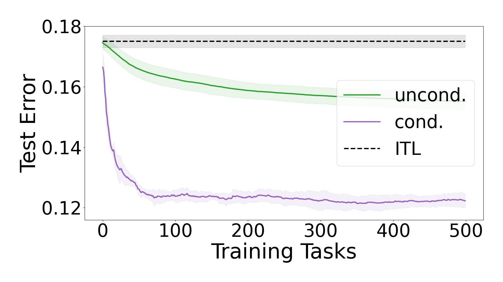
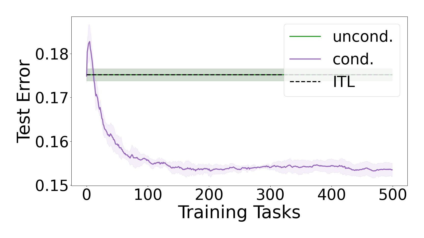
We considered two variants of the setting described in Example 1 with side information corresponding to the training datasets ZtrZ_{\rm tr} associated to each task. In both settings, we sampled Ttot=900T_{\rm tot}=900 tasks from a uniform mixture of mm clusters. For each task μ\mu, we generated the target vector wμ∈ℝdw_{\mu}\in\mathbb{R}^{d} with d=20d=20 as wμ=P⁡(jμ)​w~μw_{\mu}=P(j_{\mu})\tilde{w}_{\mu}, where, jμ∈{1,…,m}j_{\mu}\in\{1,\dots,m\} denotes the cluster from which the task μ\mu was sampled and with the components of w~μ∈ℝd/(10)\tilde{w}_{\mu}\in\mathbb{R}^{d/(10)} sampled from the Gaussian distribution 𝒢⁡(0,1)\mathcal{G}(0,1) and then w~μ\tilde{w}_{\mu} normalized to have unit norm, with P⁡(jμ)∈ℝd×d/(10)P(j_{\mu})\in\mathbb{R}^{d\times d/(10)} a matrix with orthonormal columns. We then generated the corresponding dataset (xi,yi)i=1ntot(x_{i},y_{i})_{i=1}^{n_{\rm tot}} with ntot=80n_{\rm tot}=80 according to the linear equation y=⟨x,wμ⟩+ϵy=\langle x,w_{\mu}\rangle+\epsilon, with xx sampled uniformly on the unit sphere in ℝd\mathbb{R}^{d} and ϵ\epsilon sampled from a Gaussian distribution, ϵ∼𝒢⁡(0,0.1)\epsilon\sim\mathcal{G}(0,0.1). In this setting, the operator norm of the inputs’ covariance matrix is small (equal to 1/d1/d) and the weight vectors’ covariance matrix of each single cluster is low-rank (its rank is d/(10)=2d/(10)=2). We implemented our conditional method using the feature map Φ:𝒟→ℝ2​d\Phi:\mathcal{D}\to\mathbb{R}^{2d} defined by Φ⁡(Z)=1ntr​∑i=1ntrϕ⁡(zi)\Phi(Z)=\frac{1}{{n_{\rm tr}}}\sum_{i=1}^{n_{\rm tr}}\phi(z_{i}), with ϕ⁡(zi)=vec⁡(xi​(yi,1)⊤)\phi(z_{i})={\rm vec}\big(x_{i}(y_{i},1)^{\scriptscriptstyle\top}\big), where, for any matrix A=[a1,a2]∈ℝd×2A=[a_{1},a_{2}]\in\mathbb{R}^{d\times 2} with columns a1,a2∈ℝda_{1},a_{2}\in\mathbb{R}^{d}, vec⁡(A)=(a1,a2)⊤∈ℝ2​d{\rm vec}(A)=(a_{1},a_{2})^{\scriptscriptstyle\top}\in\mathbb{R}^{2d}.

Refer to captionRefer to caption
Figure 1: Test error (averaged over 55 random generations of the data) of different methods w.r.t. an increasing number of tasks on synthetic data. 22 clusters (Left) and 66 clusters (Right).

In Fig. 1, we report the results we got on an environment of tasks generated as above with m=2m=2 (Left) and m=6m=6 (Right) clusters, respectively. As we can see, when the clusters are two, the unconditional approach outperforms ITL (as predicted from previous literature), but the unconditional method is in turn outperformed by our conditional counterpart. When the number of clusters raises to six, the performance of unconditional meta-learning degrades to the same performance of ITL, while conditional meta-learning outperforms both methods. Summarizing, the more the heterogeneity of the environment (number of clusters) is significant, the more the conditional approach brings advantage w.r.t. the unconditional one. This is in line with our statement in Example 1.
Refer to captionRefer to caption
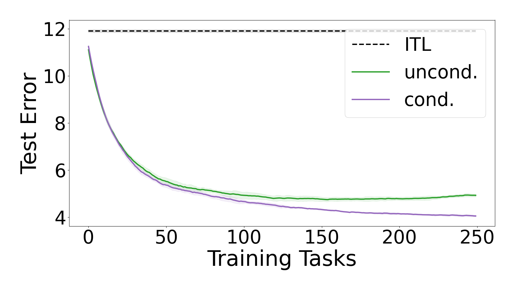
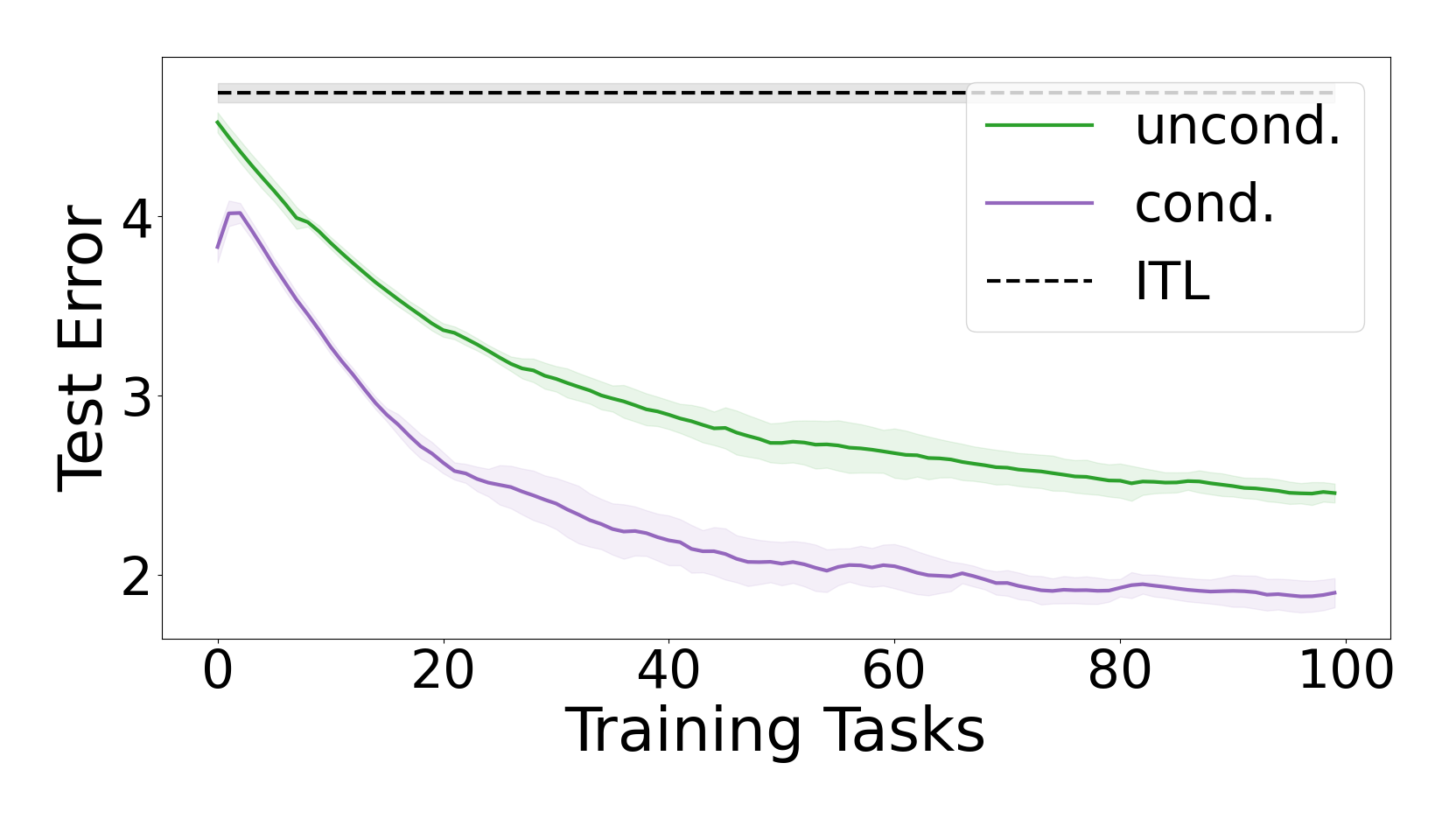
Figure 2: Test error (averaged over 55 random splitting of the data) of different methods w.r.t. an increasing number of tasks on the Lenk dataset (Left) and the Movielens-100k dataset (Right).

Refer to caption

Figure 3: Test error (averaged over 55 random splitting of the data) of different methods w.r.t. an increasing number of tasks on the Jester-1 dataset.

Real Datasets

We tested the performance of the methods also on the regression problem on the computer survey data from Lenk et al., 1996 (McDonald et al., 2016, see also). Ttot=180T_{\rm tot}=180 people (tasks) rated the likelihood of purchasing one of ntot=20n_{\rm tot}=20 computers. The input represents d=13d=13 computers’ characteristics and the label is a rate in {0,…,10}\{0,\dots,10\}. In this case, we used as side information the training datapoints Z=(zi)i=1ntrZ=(z_{i})_{i=1}^{n_{\rm tr}} and the feature map Φ:𝒟→ℝd+1\Phi:\mathcal{D}\to\mathbb{R}^{d+1} defined by Φ⁡(Z)=wZ\Phi(Z)=w_{Z}, with wZw_{Z} the solution of Tikhonov regularization with the squared loss, namely, the vector satisfying (X^⊤​X^+Id+1)​wZ=X^⊤​y(\hat{X}^{\scriptscriptstyle\top}\hat{X}+I_{d+1})w_{Z}=\hat{X}^{\scriptscriptstyle\top}y, where, X^∈ℝ(d+1)×n\hat{X}\in\mathbb{R}^{(d+1)\times n} is the matrix obtained by adding to the matrix X∈ℝn×dX\in\mathbb{R}^{n\times d} one column of ones at the end. Fig. 2 (Left) shows that also in this case, the unconditional approach outperforms ITL, but the performance of its conditional counterpart is much better.

Finally, we tested the performance of the methods on the Movielens-100k and Jester-1 real-world datasets, containing ratings of users (tasks) to movies and jokes (points), respectively. We recall that recommendation system settings with dd items can be interpreted within the meta-learning setting by considering each data point (x,y)(x,y) to have input x∈ℝdx\in\mathbb{R}^{d} to be the one-hot encoding of the current item to be rated (e.g. a movie or a joke) and y∈ℝy\in\mathbb{R} the corresponding score (see e.g. Denevi et al., 2019a, for more details). We restricted the original dataset to the ntot=20n_{\rm tot}=20 most voted movies/jokes (as a consequence, by formulation, d=20d=20). We guaranteed each user voted at least 55 movies/jokes, which led to a total of Ttot=400/450T_{\rm tot}=400/450 tasks (i.e. users). In both cases, we used as side information the training datapoints Z=(zi)i=1ntrZ=(z_{i})_{i=1}^{n_{\rm tr}}. For the Movielens-100k dataset we used the same feature map described for the synthetic clusters experiments in Fig. 1. For the Jester-1 dataset, let MM and mm denote the maximum and minimum rating value that can be assigned to a joke. We adopted the feature map Φ:𝒟→ℝ2​d+1\Phi:\mathcal{D}\to\mathbb{R}^{2d+1} such that, for any dataset Z=(xi,yi)i=1nZ=(x_{i},y_{i})_{i=1}^{n}, we have

Φ⁡(Z)=(vec​(Φ~​(Z))1),\Phi(Z)=\left(\begin{array}[]{c}\textrm{vec}(\tilde{\Phi}(Z))\\ 1\end{array}\right), (27)

where vec denotes the vectorization operator (i.e. mapping a matrix in the vector concatenating all its columns) and Φ~:Z→ℝd×2\widetilde{\Phi}:Z\to\mathbb{R}^{d\times 2} is such that

Φ~​(Z)=[cos⁡(∑i=1nxi​(π4​M−yiM−m)),sin⁡(∑i=1nxi​(π4​M−yiM−m))]⊙(∑i=1nxi),\widetilde{\Phi}(Z)=\left[\cos\left(\sum_{i=1}^{n}x_{i}\left(\frac{\pi}{4}\frac{M-y_{i}}{M-m}\right)\right),~\sin\left(\sum_{i=1}^{n}x_{i}\left(\frac{\pi}{4}\frac{M-y_{i}}{M-m}\right)\right)\right]\odot\left(\sum_{i=1}^{n}x_{i}\right), (28)

with ⊙\odot denoting the Hadamard (entry-wise) product broad-casted across both columns.

The rationale behind this feature map is to represent as similar vectors those users with similar scores for the same movies. In particular, each item-score pair observed in training is represented as a unitary vector in ℝ+⁣+2\mathbb{R}_{++}^{2}, with the angle depending on the score attributed to that item (the vector corresponds to zero if that movie was not observed at the training time). We noticed that this feature map did not provide significant advantages on the Movielens-100k dataset, while being particularly favorable on the Jester-1 benchmark.

We report the average test errors (and standard deviation) for ITL, conditional and unconditional meta-learning in Fig. 2 (Right) and Fig. 3 for Movielens-100k and Jester-1, respectively. As it can be noticed, the proposed approach performs significantly better than ITL and its unconditional counterpart. This suggests that groups of users might rely each on similar features (but different from those of other groups) to rate an item in the dataset (respectively a movie or a joke).

6 Conclusion

We proposed a conditional meta-learning approach aiming at learning a function mapping task’s side information into a linear representation that is well suited for the task at hand. We theoretically and experimentally showed that the proposed conditional approach is advantageous w.r.t. the standard unconditional counterpart when the observed tasks share heterogeneous linear representations. Our investigation allowed us to develop also a new variant of an unconditional meta-learning method requiring tuning one less hyper-parameter and relying on faster learning bounds than state-of-the-art unconditional approaches.

We identify two main directions for future work. A first question left opened by most conditional meta-learning methods is how to design a suitable feature map Φ\Phi when the tasks’ training datas is used as side information. Following most previous work Rusu et al., 2018; Wang et al., 2020 in our experiments we adopted a mean embedding representation. However, given the key importance played by such feature map in Thm. 5, it will be worth investigating better alternatives in the future. A second direction is more focused on computations and modeling aspects. In particular it will be valuable to investigate how to predict non-linear conditioning functions (similarly to e.g. Bertinetto et al., 2018; Finn et al., 2017) and develop more efficient versions of our method, using less expensive algorithms to update the positive matrices, such as the Frank-Wolfe algorithm used in Bullins et al., 2019 to deal with unconditional settings.

References

  • Abernethy et al., (2009) Abernethy, J., Bach, F., Evgeniou, T., and Vert, J.-P. (2009). A new approach to collaborative filtering: Operator estimation with spectral regularization. Journal of Machine Learning Research, 10(Mar):803–826.
  • Argyriou et al., (2008) Argyriou, A., Evgeniou, T., and Pontil, M. (2008). Convex multi-task feature learning. Machine Learning, 73(3):243–272.
  • Balcan et al., (2019) Balcan, M.-F., Khodak, M., and Talwalkar, A. (2019). Provable guarantees for gradient-based meta-learning. In International Conference on Machine Learning, pages 424–433.
  • Baxter, (2000) Baxter, J. (2000). A model of inductive bias learning. J. Artif. Intell. Res., 12(149–198):3.
  • Bertinetto et al., (2018) Bertinetto, L., Henriques, J. F., Torr, P. H., and Vedaldi, A. (2018). Meta-learning with differentiable closed-form solvers. arXiv preprint arXiv:1805.08136.
  • Bousquet and Elisseeff, (2002) Bousquet, O. and Elisseeff, A. (2002). Stability and generalization. Journal of machine learning research, 2(Mar):499–526.
  • Bullins et al., (2019) Bullins, B., Hazan, E., Kalai, A., and Livni, R. (2019). Generalize across tasks: Efficient algorithms for linear representation learning. In Algorithmic Learning Theory, pages 235–246.
  • Cai et al., (2020) Cai, T. T., Liang, T., and Rakhlin, A. (2020). Weighted message passing and minimum energy flow for heterogeneous stochastic block models with side information. Journal of Machine Learning Research, 21(11):1–34.
  • Caruana, (1997) Caruana, R. (1997). Multitask learning. Machine learning, 28(1):41–75.
  • (10) Denevi, G., Ciliberto, C., Grazzi, R., and Pontil, M. (2019a). Learning-to-learn stochastic gradient descent with biased regularization. In International Conference on Machine Learning, pages 1566–1575.
  • Denevi et al., (2018) Denevi, G., Ciliberto, C., Stamos, D., and Pontil, M. (2018). Incremental learning-to-learn with statistical guarantees. In Proc. 34th Conference on Uncertainty in Artificial Intelligence (UAI).
  • Denevi et al., (2020) Denevi, G., Pontil, M., and Ciliberto, C. (2020). The advantage of conditional meta-learning for biased regularization and fine tuning. Advances in Neural Information Processing Systems, 33.
  • (13) Denevi, G., Stamos, D., Ciliberto, C., and Pontil, M. (2019b). Online-within-online meta-learning. In Advances in Neural Information Processing Systems, pages 13089–13099.
  • Finn et al., (2017) Finn, C., Abbeel, P., and Levine, S. (2017). Model-agnostic meta-learning for fast adaptation of deep networks. In Proceedings of the 34th International Conference on Machine Learning, volume 70 of Proceedings of Machine Learning Research, pages 1126–1135. PMLR.
  • Finn and Levine, (2018) Finn, C. and Levine, S. (2018). Meta-learning and universality: Deep representations and gradient descent can approximate any learning algorithm. In International Conference on Learning Representations.
  • Finn et al., (2019) Finn, C., Rajeswaran, A., Kakade, S., and Levine, S. (2019). Online meta-learning. In International Conference on Machine Learning, pages 1920–1930.
  • Harper and Konstan, (2015) Harper, F. M. and Konstan, J. A. (2015). The movielens datasets: History and context. Acm transactions on interactive intelligent systems (tiis), 5(4):1–19.
  • Hogben, (2006) Hogben, L. (2006). Handbook of linear algebra. CRC press.
  • Hogben, (2013) Hogben, L. (2013). Handbook of linear algebra. CRC Press.
  • Jacob et al., (2009) Jacob, L., Vert, J.-p., and Bach, F. R. (2009). Clustered multi-task learning: A convex formulation. In Advances in neural information processing systems, pages 745–752.
  • Jerfel et al., (2019) Jerfel, G., Grant, E., Griffiths, T., and Heller, K. A. (2019). Reconciling meta-learning and continual learning with online mixtures of tasks. In Advances in Neural Information Processing Systems, pages 9119–9130.
  • Khodak et al., (2019) Khodak, M., Balcan, M.-F. F., and Talwalkar, A. S. (2019). Adaptive gradient-based meta-learning methods. In Advances in Neural Information Processing Systems, pages 5915–5926.
  • Lenk et al., (1996) Lenk, P. J., DeSarbo, W. S., Green, P. E., and Young, M. R. (1996). Hierarchical bayes conjoint analysis: Recovery of partworth heterogeneity from reduced experimental designs. Marketing Science, 15(2):173–191.
  • Maurer, (2009) Maurer, A. (2009). Transfer bounds for linear feature learning. Machine Learning, 75(3):327–350.
  • Maurer et al., (2013) Maurer, A., Pontil, M., and Romera-Paredes, B. (2013). Sparse coding for multitask and transfer learning. In International Conference on Machine Learning.
  • Maurer et al., (2016) Maurer, A., Pontil, M., and Romera-Paredes, B. (2016). The benefit of multitask representation learning. The Journal of Machine Learning Research, 17(1):2853–2884.
  • McDonald et al., (2016) McDonald, A. M., Pontil, M., and Stamos, D. (2016). New perspectives on k-support and cluster norms. Journal of Machine Learning Research, 17(155):1–38.
  • Micchelli et al., (2013) Micchelli, C. A., Morales, J. M., and Pontil, M. (2013). Regularizers for structured sparsity. Advances in Computational Mathematics, 38(3):455–489.
  • Pentina and Lampert, (2014) Pentina, A. and Lampert, C. (2014). A PAC-Bayesian bound for lifelong learning. In International Conference on Machine Learning, pages 991–999.
  • Rusu et al., (2018) Rusu, A. A., Rao, D., Sygnowski, J., Vinyals, O., Pascanu, R., Osindero, S., and Hadsell, R. (2018). Meta-learning with latent embedding optimization. arXiv preprint arXiv:1807.05960.
  • Shalev-Shwartz and Ben-David, (2014) Shalev-Shwartz, S. and Ben-David, S. (2014). Understanding Machine Learning: From Theory to Algorithms. Cambridge University Press.
  • Steinwart and Christmann, (2008) Steinwart, I. and Christmann, A. (2008). Support vector machines. Springer Science & Business Media.
  • Tripuraneni et al., (2020) Tripuraneni, N., Jin, C., and Jordan, M. I. (2020). Provable meta-learning of linear representations. arXiv preprint arXiv:2002.11684.
  • Vuorio et al., (2019) Vuorio, R., Sun, S.-H., Hu, H., and Lim, J. J. (2019). Multimodal model-agnostic meta-learning via task-aware modulation. In Advances in Neural Information Processing Systems, pages 1–12.
  • Wang et al., (2020) Wang, R., Demiris, Y., and Ciliberto, C. (2020). A structured prediction approach for conditional meta-learning. Advances in Neural Information Processing Systems.
  • Yao et al., (2019) Yao, H., Wei, Y., Huang, J., and Li, Z. (2019). Hierarchically structured meta-learning. arXiv preprint arXiv:1905.05301.

Appendix

The supplementary material is organized as follows. In Appendix A we give the bound on the generalization error of the algorithm in Eq. 2 that we used in various proofs. In Appendix B we report the proof to get the closed form of the best conditioning function τρ\tau_{\rho} outlined in Prop. 2. In Appendix C we report the proof of the statement in Example 1. In Appendix D, we report the proofs of the statements we used in Section 4 in order to prove the expected excess risk bound in Thm. 5 for Algorithm 1. Finally, in Appendix E we report the experimental details we missed in the main body.

Appendix A Generalization Bound of the Within-Task Algorithm

We now study the generalization error of the within-task algorithm in Eq. 2, i.e. the discrepancy between the (true) risk and the empirical risk of the corresponding estimator. This is done in the following result where we exploit stability arguments, more precisely the so-called hypothesis stability, see (Bousquet and Elisseeff, 2002, Def. 33).

Proposition 6 (Generalization Error of the Within-Task Algorithm in Eq. 2).

Let Asm. 1 hold. For a distribution μ∼ρ\mu\sim\rho, fix a dataset Z=(xi,yi)i=1n∼μnZ=(x_{i},y_{i})_{i=1}^{n}\sim\mu^{n}. For any θ∈Θ\theta\in\Theta, let wθ​(Z)w_{\theta}(Z) be the corresponding RERM in Eq. 2 over ZZ. Then, the following generalization error bound holds for wθ​(Z)w_{\theta}(Z):

𝔼Z∼μn​[ℛμ​(wθ​(Z))−ℛZ​(wθ​(Z))]≤2​L2n​Tr​(𝔼z∼μ​θ​x​x⊤).\mathbb{E}_{Z\sim\mu^{n}}~\big[\mathcal{R}_{\mu}(w_{\theta}(Z))-\mathcal{R}_{Z}(w_{\theta}(Z))\big]\leq\frac{2L^{2}}{n}~\text{\rm Tr}\big(\mathbb{E}_{z\sim\mu}~\theta xx^{\scriptscriptstyle\top}\big). (29)
Proof.

During this proof, we need to make explicit the dependency of the RERM (Regularized Empirical Risk Minimizer) wθw_{\theta} in Eq. 2 w.r.t. the dataset ZZ. For any i∈{1,…,n}i\in\{1,\dots,n\}, consider the dataset Z(i)Z^{(i)}, a copy of the original dataset ZZ in which we exchange the point zi=(xi,yi)z_{i}=(x_{i},y_{i}) with a new i.i.d. point zi′=(xi′,yi′)z_{i}^{\prime}=(x_{i}^{\prime},y_{i}^{\prime}). For a fixed θ∈Θ\theta\in\Theta, we analyze how much this perturbation affects the outputs of the RERM algorithm in Eq. 2. In other words, we study the discrepancy between wθ​(Z)w_{\theta}(Z) and wθ​(Z(i))w_{\theta}(Z^{(i)}). We start from observing that, since by Asm. 1 ℛZ,θ\mathcal{R}_{Z,\theta} is 11-strongly convex w.r.t. ∥⋅∥θ=⟨⋅,θ†⋅⟩\|\cdot\|_{\theta}=\sqrt{\big\langle\cdot,\theta^{\dagger}\cdot\big\rangle}, by growth condition and the definition of the RERM algorithm, we can write the following

12​‖wθ​(Z(i))−wθ​(Z)‖θ2≤ℛZ,θ​(wθ​(Z(i)))−ℛZ,θ​(wθ​(Z))12​‖wθ​(Z(i))−wθ​(Z)‖θ2≤ℛZ(i),θ​(wθ​(Z))−ℛZ(i),θ​(wθ​(Z(i))).\begin{split}&\frac{1}{2}~\big\|w_{\theta}(Z^{(i)})-w_{\theta}(Z)\big\|_{\theta}^{2}\leq\mathcal{R}_{Z,\theta}(w_{\theta}(Z^{(i)}))-\mathcal{R}_{Z,\theta}(w_{\theta}(Z))\\ &\frac{1}{2}~\big\|w_{\theta}(Z^{(i)})-w_{\theta}(Z)\big\|_{\theta}^{2}\leq\mathcal{R}_{Z^{(i)},\theta}(w_{\theta}(Z))-\mathcal{R}_{Z^{(i)},\theta}(w_{\theta}(Z^{(i)})).\end{split} (30)

Hence, summing the two inequalities above, we get

‖wθ​(Z(i))−wθ​(Z)‖θ2≤ℛZ,θ​(wθ​(Z(i)))−ℛZ(i),θ​(wθ​(Z(i)))+ℛZ(i),θ​(wθ​(Z))−ℛZ,θ​(wθ​(Z))=A+Bn,\begin{split}\big\|w_{\theta}(Z^{(i)})-w_{\theta}(Z)\big\|_{\theta}^{2}&\leq\mathcal{R}_{Z,\theta}(w_{\theta}(Z^{(i)}))-\mathcal{R}_{Z^{(i)},\theta}(w_{\theta}(Z^{(i)}))+\mathcal{R}_{Z^{(i)},\theta}(w_{\theta}(Z))-\mathcal{R}_{Z,\theta}(w_{\theta}(Z))\\ &=\frac{{\text{A}}+{\text{B}}}{n},\end{split} (31)

where we have introduced the terms

A=ℓ⁡(⟨xi′,wθ​(Z)⟩,yi′)−ℓ⁡(⟨xi′,wθ​(Z(i))⟩,yi′)B=ℓ⁡(⟨xi,wθ​(Z(i))⟩,yi)−ℓ⁡(⟨xi,wθ​(Z)⟩,yi).\begin{split}&\text{A}=\ell(\langle x_{i}^{\prime},w_{\theta}(Z)\rangle,y_{i}^{\prime})-\ell(\langle x_{i}^{\prime},w_{\theta}(Z^{(i)})\rangle,y_{i}^{\prime})\\ &\text{B}=\ell(\langle x_{i},w_{\theta}(Z^{(i)})\rangle,y_{i})-\ell(\langle x_{i},w_{\theta}(Z)\rangle,y_{i}).\end{split} (32)

Now, introducing the subgradients sθ,i′∈∂ℓ⁡(⋅,yi′)​(⟨xi′,wθ​(Z)⟩)s_{\theta,i}^{\prime}\in\partial\ell(\cdot,y_{i}^{\prime})(\langle x_{i}^{\prime},w_{\theta}(Z)\rangle) and sθ,i∈∂ℓ⁡(⋅,yi)​(⟨xi,wθ​(Z(i))⟩)s_{\theta,i}\in\partial\ell(\cdot,y_{i})(\langle x_{i},w_{\theta}(Z^{(i)})\rangle) and applying Holder’s inequality, we can write

A≤⟨xi′​sθ,i′,wθ​(Z)−wθ​(Z(i))⟩≤‖xi′​sθ,i′‖θ,∗​‖wθ​(Z(i))−wθ​(Z)‖θB≤⟨xi​sθ,i,wθ​(Z(i))−wθ​(Z)⟩≤‖xi​sθ,i‖θ,∗​‖wθ​(Z(i))−wθ​(Z)‖θ,\begin{split}&\text{A}\leq\big\langle x_{i}^{\prime}s_{\theta,i}^{\prime},w_{\theta}(Z)-w_{\theta}(Z^{(i)})\big\rangle\leq\big\|x_{i}^{\prime}s_{\theta,i}^{\prime}\big\|_{\theta,*}~\big\|w_{\theta}(Z^{(i)})-w_{\theta}(Z)\big\|_{\theta}\\ &\text{B}\leq\big\langle x_{i}s_{\theta,i},w_{\theta}(Z^{(i)})-w_{\theta}(Z)\big\rangle\leq\big\|x_{i}s_{\theta,i}\big\|_{\theta,*}~\big\|w_{\theta}(Z^{(i)})-w_{\theta}(Z)\big\|_{\theta},\end{split} (33)

where ∥⋅∥θ,∗=⟨⋅,θ⋅⟩\|\cdot\|_{\theta,*}=\sqrt{\big\langle\cdot,\theta\cdot\big\rangle} is the dual norm of ∥⋅∥θ\|\cdot\|_{\theta}. Combining these last two inequalities with Eq. 31 and simplifying, we get the following

‖wθ​(Z(i))−wθ​(Z)‖θ≤1n​(‖xi′​sθ,i′‖θ,∗+‖xi​sθ,i‖θ,∗).\big\|w_{\theta}(Z^{(i)})-w_{\theta}(Z)\big\|_{\theta}\leq\frac{1}{n}\Bigl(\big\|x_{i}^{\prime}s_{\theta,i}^{\prime}\big\|_{\theta,*}+\big\|x_{i}s_{\theta,i}\big\|_{\theta,*}\Bigr). (34)

Hence, combining the first row in Eq. 33 with Eq. 34, we can write

ℓ⁡(⟨xi′,wθ​(Z)⟩,yi′)−ℓ⁡(⟨xi′,wθ​(Z(i))⟩,yi′)≤1n​(‖xi′​sθ,i′‖θ,∗2+‖xi′​sθ,i′‖θ,∗​‖xi​sθ,i‖θ,∗).\begin{split}\ell(\langle x_{i}^{\prime},w_{\theta}(Z)\rangle,y_{i}^{\prime})-\ell(\langle x_{i}^{\prime},w_{\theta}(Z^{(i)})\rangle,y_{i}^{\prime})\leq\frac{1}{n}\Bigl(\big\|x_{i}^{\prime}s_{\theta,i}^{\prime}\big\|_{\theta,*}^{2}+\big\|x_{i}^{\prime}s_{\theta,i}^{\prime}\big\|_{\theta,*}~\big\|x_{i}s_{\theta,i}\big\|_{\theta,*}\Bigr).\end{split} (35)

Now, taking the expectation w.r.t. Z∼μnZ\sim\mu^{n} and zi′∼μz_{i}^{\prime}\sim\mu of the left side member above, according to (Bousquet and Elisseeff, 2002, Lemma 77), we get

𝔼Z∼μn​𝔼zi′∼μ​[ℓ⁡(⟨xi′,wθ​(Z)⟩,yi′)−ℓ⁡(⟨xi′,wθ​(Z(i))⟩,yi′)]=𝔼Z∼μn​[ℛμ​(wθ​(Z))−ℛZ​(wθ​(Z))].\mathbb{E}_{Z\sim\mu^{n}}~\mathbb{E}_{z_{i}^{\prime}\sim\mu}~\Big[\ell(\langle x_{i}^{\prime},w_{\theta}(Z)\rangle,y_{i}^{\prime})-\ell(\langle x_{i}^{\prime},w_{\theta}(Z^{(i)})\rangle,y_{i}^{\prime})\Big]=\mathbb{E}_{Z\sim\mu^{n}}~\Big[\mathcal{R}_{\mu}(w_{\theta}(Z))-\mathcal{R}_{Z}(w_{\theta}(Z))\Big].

Finally, taking the expectation of the right side member, exploiting the fact that the points are i.i.d. according μ\mu, we get

𝔼Z∼μn​𝔼zi′∼μ​1n​(‖xi′​sθ,i′‖θ,∗2+‖xi′​sθ,i′‖θ,∗​‖xi​sθ,i‖θ,∗)≤2n​𝔼Z∼μn​𝔼zi′∼μ​‖xi′​sθ,i′‖θ,∗2,\mathbb{E}_{Z\sim\mu^{n}}~\mathbb{E}_{z_{i}^{\prime}\sim\mu}~\frac{1}{n}\Bigg(\big\|x_{i}^{\prime}s_{\theta,i}^{\prime}\big\|_{\theta,*}^{2}+\big\|x_{i}^{\prime}s_{\theta,i}^{\prime}\big\|_{\theta,*}\big\|x_{i}s_{\theta,i}\big\|_{\theta,*}\Bigg)\leq\frac{2}{n}~\mathbb{E}_{Z\sim\mu^{n}}~\mathbb{E}_{z_{i}^{\prime}\sim\mu}~\big\|x_{i}^{\prime}s_{\theta,i}^{\prime}\big\|_{\theta,*}^{2}, (36)

where we recall that sθ,i′∈∂ℓ⁡(⋅,yi′)​(⟨xi′,wθ​(Z)⟩)s_{\theta,i}^{\prime}\in\partial\ell(\cdot,y_{i}^{\prime})(\langle x_{i}^{\prime},w_{\theta}(Z)\rangle). Combining the two last statements above, we get

𝔼Z∼μn​[ℛμ​(wθ​(Z))−ℛZ​(wθ​(Z))]≤2n​𝔼Z∼μn​𝔼zi′∼μ​‖xi′​sθ,i′‖θ,∗2.\mathbb{E}_{Z\sim\mu^{n}}~\big[\mathcal{R}_{\mu}(w_{\theta}(Z))-\mathcal{R}_{Z}(w_{\theta}(Z))\big]\leq\frac{2}{n}~\mathbb{E}_{Z\sim\mu^{n}}~\mathbb{E}_{z_{i}^{\prime}\sim\mu}~\big\|x_{i}^{\prime}s_{\theta,i}^{\prime}\big\|_{\theta,*}^{2}. (37)

Finally, substituting the close form of ∥⋅∥θ,∗\|\cdot\|_{\theta,*} and observing that, by Asm. 1 we have ‖xi′​sθ,i′‖θ,∗2≤L2​‖xi′‖θ,∗2\big\|x_{i}^{\prime}s_{\theta,i}^{\prime}\big\|_{\theta,*}^{2}\leq L^{2}\big\|x_{i}^{\prime}\big\|_{\theta,*}^{2}, we get the desired statement:

𝔼Z∼μn​[ℛμ​(wθ​(Z))−ℛZ​(wθ​(Z))]≤2​L2n​𝔼zi′∼μ​⟨xi′,θ​xi′⟩=2​L2n​Tr​(𝔼z∼μ​θ​x​x⊤).\mathbb{E}_{Z\sim\mu^{n}}~\big[\mathcal{R}_{\mu}(w_{\theta}(Z))-\mathcal{R}_{Z}(w_{\theta}(Z))\big]\leq\frac{2L^{2}}{n}~\mathbb{E}_{z_{i}^{\prime}\sim\mu}~\big\langle x_{i}^{\prime},\theta x_{i}^{\prime}\big\rangle=\frac{2L^{2}}{n}~\text{\rm Tr}\big(\mathbb{E}_{z\sim\mu}~\theta xx^{\scriptscriptstyle\top}\big). (38)

∎

Appendix B Proof of Prop. 2

In this section we report the proof to get the closed form of the best conditioning function τρ\tau_{\rho} outlined in Prop. 2. In order to do this, we need the following results.

Lemma 7.

For any μ∼ρℳ\mu\sim{\rho_{\mathcal{M}}}, define the inputs’ covariance matrix Cμ=𝔼x∼ημ​x​x⊤C_{\mu}=\mathbb{E}_{x\sim\eta_{\mu}}xx^{\scriptscriptstyle\top}. Then, for any wμ∈argminw∈ℝdℛμ​(w)w_{\mu}\in\operatornamewithlimits{argmin}_{w\in\mathbb{R}^{d}}\mathcal{R}_{\mu}(w), the projection w0,μ=Cμ†​Cμ​wμw_{0,\mu}=C_{\mu}^{\dagger}C_{\mu}w_{\mu} of wμw_{\mu} onto the range of CμC_{\mu} is still a minimizer of ℛμ\mathcal{R}_{\mu}.

Proof.

Consider the decomposition of wμw_{\mu} w.r.t. the range of CμC_{\mu}:

wμ=w0,μ+w⟂w_{\mu}=w_{0,\mu}+w^{\perp} (39)

with w0,μ=Cμ†​Cμ​wμw_{0,\mu}=C_{\mu}^{\dagger}C_{\mu}w_{\mu} and w⟂∈ℝdw^{\perp}\in\mathbb{R}^{d} such that Cμ​w⟂=0C_{\mu}w^{\perp}=0. We note that, almost surely w.r.t. the points x∈ℝdx\in\mathbb{R}^{d} sampled from μ\mu, we have ⟨w⟂,x⟩=0\left\langle{w^{\perp}},{x}\right\rangle=0. This follows by noting that by the orthogonality between CμC_{\mu} and w⟂w^{\perp}, we have

0=⟨w⟂,Cμ​w⟂⟩=𝔼x∼ημ​⟨w⟂,x​x⊤​w⟂⟩=𝔼x∼ημ​⟨x,w⟂⟩2,0=\left\langle{w^{\perp}},{C_{\mu}w^{\perp}}\right\rangle=\mathbb{E}_{x\sim\eta_{\mu}}\left\langle{w^{\perp}},{xx^{\scriptscriptstyle\top}w^{\perp}}\right\rangle=\mathbb{E}_{x\sim\eta_{\mu}}\left\langle{x},{w^{\perp}}\right\rangle^{2}, (40)

that can hold only if ⟨x,w⟂⟩2=0\left\langle{x},{w^{\perp}}\right\rangle^{2}=0 almost surely (a.s.) w.r.t. ημ\eta_{\mu}. We conclude that ⟨wμ,x⟩=⟨w0,μ,x⟩+⟨w⟂,x⟩=⟨w0,μ,x⟩\left\langle{w_{\mu}},{x}\right\rangle=\left\langle{w_{0,\mu}},{x}\right\rangle+\left\langle{w^{\perp}},{x}\right\rangle=\left\langle{w_{0,\mu}},{x}\right\rangle a.s. w.r.t. μ\mu and, consequently, ℛμ​(wμ)=ℛμ​(w0,μ)\mathcal{R}_{\mu}(w_{\mu})=\mathcal{R}_{\mu}(w_{0,\mu}). ∎

Corollary 8.

For any s∈𝒮s\in\mathcal{S}, recall the conditional covariance matrices in Thm. 1. Then, Ran​(W​(s))⊂Ran​(C​(s))\text{\rm Ran}(W(s))\subset\text{\rm Ran}(C(s)), namely the range of the task-vector conditional covariance W⁡(s)W(s) is always contained in the range of the input conditional covariance C⁡(s)C(s).

Proof.

The corollary is a direct consequence of the previous Lemma 7. The result above guarantees that for any μ∼ρℳ\mu\sim{\rho_{\mathcal{M}}}, the rank-one operator Wμ=wμ​wμ⊤W_{\mu}=w_{\mu}w_{\mu}^{\scriptscriptstyle\top} has range contained in the range of CμC_{\mu}. Taking the conditional expectations W(s)=𝔼μ∼ρ(⋅|s)WμW(s)=\mathbb{E}_{\mu\sim\rho(\cdot|s)}W_{\mu} and C(s)=𝔼μ∼ρ(⋅|s)CμC(s)=\mathbb{E}_{\mu\sim\rho(\cdot|s)}C_{\mu} maintains this relation unaltered, giving the desired statement. ∎

Lemma 9.

Let P∈𝕊+dP\in\mathbb{S}_{+}^{d} be an orthogonal projector, namely such that P=P2P=P^{2}. Then, for any positive definite matrix θ∈𝕊+⁣+d\theta\in\mathbb{S}_{++}^{d}, we have P​θ−1​P⪰(P​θ​P)†P\theta^{-1}P\succeq(P\theta P)^{\dagger}.

Proof.

The proof is essentially a corollary of Schur’s complement. Let consider the decomposition

θ=P​θ​P⏟A+P​θ​(I−P)⏟B+(I−P)​θ​P⏟B⊤+(I−P)​θ​(I−P)⏟C\theta=\underbrace{P\theta P}_{A}+\underbrace{P\theta(I-P)}_{B}+\underbrace{(I-P)\theta P}_{B^{\scriptscriptstyle\top}}+\underbrace{(I-P)\theta(I-P)}_{C} (41)

where A,C∈𝕊+dA,C\in\mathbb{S}_{+}^{d}, B∈ℝd×dB\in\mathbb{R}^{d\times d} and C​B=B⊤​C=0CB=B^{\scriptscriptstyle\top}C=0 since (I−P)​P=P⁡(I−P)=P−P2=P−P=0(I-P)P=P(I-P)=P-P^{2}=P-P=0. Additionally, since C†=C​C†​C†=C†​C†​CC^{\dagger}=CC^{\dagger}C^{\dagger}=C^{\dagger}C^{\dagger}C, we have that also A​C†=A​C​C†​C†=0AC^{\dagger}=ACC^{\dagger}C^{\dagger}=0 and analogously C†​B=B⊤​C†=0C^{\dagger}B=B^{\scriptscriptstyle\top}C^{\dagger}=0. Note that since θ\theta is invertible, both AA and CC are full rank. We now observe a few relevant interactions between the objects above. In particular, we observe that C​C†​B⊤=B⊤CC^{\dagger}B^{\scriptscriptstyle\top}=B^{\scriptscriptstyle\top}. To see this, first note that

C​C†​B⊤=(I−P)​θ​(I−P)​((I−P)​θ​(I−P))†​(I−P)​θ​P.CC^{\dagger}B^{\scriptscriptstyle\top}=(I-P)\theta(I-P)\big((I-P)\theta(I-P)\big)^{\dagger}(I-P)\theta P. (42)

By taking D=(I−P)​θ1/2D=(I-P)\theta^{1/2} and using the properties of the pseudoinverse (e.g. D=D⊤​(D​D⊤)†D=D^{\scriptscriptstyle\top}(DD^{\scriptscriptstyle\top})^{\dagger}), we have

C​C†​B⊤\displaystyle CC^{\dagger}B^{\scriptscriptstyle\top} =D​D⊤​(D​D⊤)†​D​θ1/2​P\displaystyle=DD^{\scriptscriptstyle\top}(DD^{\scriptscriptstyle\top})^{\dagger}D\theta^{1/2}P (43)
=D​D†​D​θ1/2​P\displaystyle=DD^{\dagger}D\theta^{1/2}P (44)
=D​θ1/2​P\displaystyle=D\theta^{1/2}P (45)
=B⊤.\displaystyle=B^{\scriptscriptstyle\top}. (46)

We now derive an alternative characterization of θ\theta in terms of A,B,CA,B,C. By adding and removing a term B​C†​BBC^{\dagger}B to θ\theta, we have

θ\displaystyle\theta =A+B+B⊤+C\displaystyle=A+B+B^{\scriptscriptstyle\top}+C (47)
=A−B​C†​B⊤+B​C†​B⊤+B+B⊤+C\displaystyle=A-BC^{\dagger}B^{\scriptscriptstyle\top}+BC^{\dagger}B^{\scriptscriptstyle\top}+B+B^{\scriptscriptstyle\top}+C (48)
=A−B​C†​B⊤+B+C+(B+C)​(C†​B⊤)\displaystyle=A-BC^{\dagger}B^{\scriptscriptstyle\top}+B+C+(B+C)(C^{\dagger}B^{\scriptscriptstyle\top}) (49)
=A−B​C†​B⊤+B+C+(A−B​C†​B⊤+B+C)​(C†​B)\displaystyle=A-BC^{\dagger}B^{\scriptscriptstyle\top}+B+C+(A-BC^{\dagger}B^{\scriptscriptstyle\top}+B+C)(C^{\dagger}B) (50)
=(A−B​C†​B⊤+B+C)​(I+C†​B⊤),\displaystyle=(A-BC^{\dagger}B^{\scriptscriptstyle\top}+B+C)(I+C^{\dagger}B^{\scriptscriptstyle\top}), (51)

where we have first used the equality C​C†​B⊤=B⊤CC^{\dagger}B^{\scriptscriptstyle\top}=B^{\scriptscriptstyle\top} and then the ortogonality A​C†=B⊤​C†=0AC^{\dagger}=B^{\scriptscriptstyle\top}C^{\dagger}=0. Following a similar reasoning

A−B​C†​B⊤+B+C\displaystyle A-BC^{\dagger}B^{\scriptscriptstyle\top}+B+C =A−B​C†​B⊤+C+B​C†​C\displaystyle=A-BC^{\dagger}B^{\scriptscriptstyle\top}+C+BC^{\dagger}C (52)
=A−B​C†​B⊤+C+B​C†​(A−B​C†​B⊤+C)\displaystyle=A-BC^{\dagger}B^{\scriptscriptstyle\top}+C+BC^{\dagger}(A-BC^{\dagger}B^{\scriptscriptstyle\top}+C) (53)
=(I+B​C†)​(A−B​C†​B⊤+C)\displaystyle=(I+BC^{\dagger})(A-BC^{\dagger}B^{\scriptscriptstyle\top}+C) (54)

since B​C†​C=CBC^{\dagger}C=C (following the same reasoning used for B⊤=C​C†​B⊤B^{\scriptscriptstyle\top}=CC^{\dagger}B^{\scriptscriptstyle\top}) and A​C†=C†​B=0AC^{\dagger}=C^{\dagger}B=0. We conclude that

θ=(I+B​C†)​(A−B​C†​B⊤+C)​(I+C†​B⊤).\theta=(I+BC^{\dagger})(A-BC^{\dagger}B^{\scriptscriptstyle\top}+C)(I+C^{\dagger}B^{\scriptscriptstyle\top}). (55)

We now show that all terms in the equation above are invertible. First note that (I+B​C†)−1=(I−B​C†)(I+BC^{\dagger})^{-1}=(I-BC^{\dagger}) and (I+C†​B⊤)−1=(I+C†​B⊤)(I+C^{\dagger}B^{\scriptscriptstyle\top})^{-1}=(I+C^{\dagger}B^{\scriptscriptstyle\top}). Moreover, since θ≻0\theta\succ 0 and C⁡(A−B​C†​B⊤)=0C(A-BC^{\dagger}B^{\scriptscriptstyle\top})=0, then also A−B​C†​B⊤≻0A-BC^{\dagger}B^{\scriptscriptstyle\top}\succ 0. We have

θ−1=(I−C†​B⊤)​(A−B​C†​B⊤+C)−1​(I−B​C†),\theta^{-1}=(I-C^{\dagger}B^{\scriptscriptstyle\top})(A-BC^{\dagger}B^{\scriptscriptstyle\top}+C)^{-1}(I-BC^{\dagger}), (56)

from which we conclude

P​θ−1​P\displaystyle P\theta^{-1}P =P​(A−B​C†​B⊤+C)−1​P\displaystyle=P(A-BC^{\dagger}B^{\scriptscriptstyle\top}+C)^{-1}P (57)
=P⁡((A−B​C†​B⊤)†+C†)​P\displaystyle=P\Big((A-BC^{\dagger}B^{\scriptscriptstyle\top})^{\dagger}+C^{\dagger}\Big)P (58)
=P​(A−B​C†​B⊤)†​P\displaystyle=P(A-BC^{\dagger}B^{\scriptscriptstyle\top})^{\dagger}P (59)
=(A−B​C†​B⊤)†.\displaystyle=(A-BC^{\dagger}B^{\scriptscriptstyle\top})^{\dagger}. (60)

Since B​C†​B⊤⪰0BC^{\dagger}B^{\scriptscriptstyle\top}\succeq 0, we have A−B​C†​B⊤⪯AA-BC^{\dagger}B^{\scriptscriptstyle\top}\preceq A and therefore (A−B​C†​B⊤)†⪰A†(A-BC^{\dagger}B^{\scriptscriptstyle\top})^{\dagger}\succeq A^{\dagger} from which we have

P​θ−1​P=(A−B​C†​B⊤)†⪰A†=(P​θ​P)†,P\theta^{-1}P=(A-BC^{\dagger}B^{\scriptscriptstyle\top})^{\dagger}\succeq A^{\dagger}=(P\theta P)^{\dagger}, (61)

as desired. ∎

Proposition 10.

Consider two matrices A,B∈𝕊+dA,B\in\mathbb{S}_{+}^{d} such that Ran​(A)⊆Ran​(B)\text{\rm Ran}(A)\subseteq\text{\rm Ran}(B) and consider the following associated problem:

minθ∈𝕊+d,Ran​(A)⊆Ran​(θ)⁡Tr​(θ−1​A)+Tr​(θ​B).\min_{\theta\in\mathbb{S}_{+}^{d},~\text{\rm Ran}(A)\subseteq\text{\rm Ran}(\theta)}~\text{\rm Tr}(\theta^{-1}A)+\text{\rm Tr}(\theta B). (62)

Then, a minimizer and the corresponding minimum of the problem above are given by

θ∗=B−1/2(B1/2AB1/2)1/2B−1/22∥B1/2A1/2∥∗.\theta_{*}=B^{-1/2}(B^{1/2}AB^{1/2})^{1/2}B^{-1/2}\quad\quad 2\big\|B^{1/2}A^{1/2}\big\|_{*}. (63)

Moreover θ∗\theta_{*} is the unique minimizer such that Ran​(θ∗)⊂Ran​(B)\text{\rm Ran}(\theta_{*})\subset\text{\rm Ran}(B).

Proof.

Let Θ={θ∈𝕊+d|Ran​(A)⊂Ran​(θ)}\Theta=\{\theta\in\mathbb{S}_{+}^{d}~|~\text{\rm Ran}(A)\subset\text{\rm Ran}(\theta)\} and denote by F:Θ→ℝF:\Theta\to\mathbb{R} the objective functional of the problem in Eq. 62, such that for any θ∈Θ\theta\in\Theta

F⁡(θ)=Tr​(θ−1​A)+Tr​(θ​B).F(\theta)=\text{\rm Tr}(\theta^{-1}A)+\text{\rm Tr}(\theta B). (64)

Note that the sign of inverse is well defined since Ran​(A)⊂Ran​(θ)\text{\rm Ran}(A)\subset\text{\rm Ran}(\theta). We begin the proof by showing that the Eq. 62 is equivalent to

minθ∈𝕊+d,Ran​(A)⊂Ran​(θ)⊂Ran​(B)⁡Tr​(θ−1​A)+Tr​(θ​B).\min_{\theta\in\mathbb{S}_{+}^{d},~\text{\rm Ran}(A)\subset\text{\rm Ran}(\theta)\subset\text{\rm Ran}(B)}~\text{\rm Tr}(\theta^{-1}A)+\text{\rm Tr}(\theta B). (65)

To see this, let P=B​B†P=BB^{\dagger} the orthogonal projector onto the range of BB. By hypothesis, A=P​A​PA=PAP and B=P​B​PB=PBP. Therefore, for any θ∈𝕊+⁣+d\theta\in\mathbb{S}_{++}^{d}

F⁡(θ)\displaystyle F(\theta) =Tr​(θ−1​A)+Tr​(θ​B)\displaystyle=\text{\rm Tr}(\theta^{-1}A)+\text{\rm Tr}(\theta B)
=Tr​(P​θ−1​P​A)+Tr​(P​θ​P​B)\displaystyle=\text{\rm Tr}(P\theta^{-1}PA)+\text{\rm Tr}(P\theta PB)
≥Tr​((P​θ​P)†​A)+Tr​(P​θ​P​B)\displaystyle\geq\text{\rm Tr}((P\theta P)^{\dagger}A)+\text{\rm Tr}(P\theta PB)
=F⁡(P​θ​P),\displaystyle=F(P\theta P),

where we have applied the fact that P​θ−1​P⪰(P​θ​P)†P\theta^{-1}P\succeq(P\theta P)^{\dagger} from Lemma 9 and the positive semidefinteness of AA. The inequality above implies the equivalence between Eq. 62 and Eq. 65. Indeed, let θ∗∈Θ\theta_{*}\in\Theta be a minimizer of Eq. 62 and consider a sequence (θn)n∈ℕ(\theta_{n})_{n\in\mathbb{N}} such that θn∈𝕊+⁣+d\theta_{n}\in\mathbb{S}_{++}^{d} for any n∈ℕn\in\mathbb{N} and θn→θ∗\theta_{n}\to\theta_{*}. By continuity of FF we have also that F⁡(θn)→F⁡(θ∗)F(\theta_{n})\to F(\theta_{*}). Clearly, F⁡(θ∗)≤F⁡(P​θn​P)≤F⁡(θn)F(\theta_{*})\leq F(P\theta_{n}P)\leq F(\theta_{n}) and therefore also F⁡(P​θn​P)→F⁡(θ∗)F(P\theta_{n}P)\to F(\theta_{*}). By continuity of FF over Θ\Theta, this also implies that the limit limn→+∞P​θn​P=P​θ∗​P\lim_{n\to+\infty}P\theta_{n}P=P\theta_{*}P is a minimizer for Eq. 62 (and one such that Ran​(θ∗)⊂Ran​(B)\text{\rm Ran}(\theta_{*})\subset\text{\rm Ran}(B)). We consider now the set ΘB={θ∈𝕊+d|Ran​(θ)=Ran​(B)}\Theta_{B}=\{\theta\in\mathbb{S}_{+}^{d}~|~\text{\rm Ran}(\theta)=\text{\rm Ran}(B)\} of all positive semidefinite matrices with same range as BB, hence invertible on Ran​(B)\text{\rm Ran}(B). Note that ΘB\Theta_{B} is an open subset of Θ\Theta and its closure in Θ\Theta corresponds to Θ\Theta itself. By definition, any θ∈ΘB\theta\in\Theta_{B} is such that θ=B†/2XB†/2\theta=B^{\dagger/2}XB^{\dagger/2} with Ran​(X)=Ran​(B)\text{\rm Ran}(X)=\text{\rm Ran}(B). This implies in particular that X​B†​B=XXB^{\dagger}B=X and θ†=B†/2X†B†/2\theta^{\dagger}=B^{\dagger/2}X^{\dagger}B^{\dagger/2}. Therefore,

F⁡(θ)\displaystyle F(\theta) =Tr​(θ†​A)+Tr​(θ​B)\displaystyle=\text{\rm Tr}(\theta^{\dagger}A)+\text{\rm Tr}(\theta B) (66)
=Tr​(X†​B1/2​A​B1/2)+Tr​(X),\displaystyle=\text{\rm Tr}(X^{\dagger}B^{1/2}AB^{1/2})+\text{\rm Tr}(X), (67)

and Ran​(B1/2​A​B1/2)⊆Ran​(B)=Ran​(X)\text{\rm Ran}(B^{1/2}AB^{1/2})\subseteq\text{\rm Ran}(B)=\text{\rm Ran}(X). We can now minimize the problem w.r.t. XX, namely

minX∈𝕊+d,Ran​(B1/2​A​B1/2)⊆Ran​(X)⁡Tr​(X†​B1/2​A​B1/2)+Tr​(X).\min_{X\in\mathbb{S}_{+}^{d},~\text{\rm Ran}(B^{1/2}AB^{1/2})\subseteq\text{\rm Ran}(X)}~\text{\rm Tr}(X^{\dagger}B^{1/2}AB^{1/2})+\text{\rm Tr}(X). (68)

The minimization corresponds to the variational form of the trace norm of B1/2​A​B1/2B^{1/2}AB^{1/2} Micchelli et al., 2013 and has solution X∗=(B1/2​A​B1/2)1/2X_{*}=(B^{1/2}AB^{1/2})^{1/2}, with minimum corresponding to 2​Tr​((B1/2​A​B1/2)1/2)=2​‖B1/2​A1/2‖∗2\text{\rm Tr}((B^{1/2}AB^{1/2})^{1/2})=2\left\|{B^{1/2}A^{1/2}}\right\|_{*}. To conclude the proof, let G:{X∈𝕊+d|Ran​(B1/2​A​B1/2)⊆Ran​(X)}→ℝG:\{X\in\mathbb{S}_{+}^{d}~|~\text{\rm Ran}(B^{1/2}AB^{1/2})\subseteq\text{\rm Ran}(X)\}\to\mathbb{R} be the objective functional in Eq. 68 such that G⁡(X)=Tr​(X†​B1/2​A​B1/2)+Tr​(X)G(X)=\text{\rm Tr}(X^{\dagger}B^{1/2}AB^{1/2})+\text{\rm Tr}(X). Let now X∗∈𝕊+dX_{*}\in\mathbb{S}_{+}^{d} be a minimzer for GG and (Xn)n∈ℕ(X_{n})_{n\in\mathbb{N}} be a minimizing sequence with Ran​(Xn)=Ran​(B)\text{\rm Ran}(X_{n})=\text{\rm Ran}(B) for each n∈ℕn\in\mathbb{N} and Xn→X∗X_{n}\to X_{*}. Let (θn)n∈ℕ(\theta_{n})_{n\in\mathbb{N}} such that θn=B†/2XB†/2\theta_{n}=B^{\dagger/2}XB^{\dagger/2} for any n∈ℕn\in\mathbb{N}. Then we have θn→B†/2X∗B†/2\theta_{n}\to B^{\dagger/2}X_{*}B^{\dagger/2} and by continuity F(B†/2X∗B†/2)=G(X∗)F(B^{\dagger/2}X_{*}B^{\dagger/2})=G(X_{*}), hence minX⁡G⁡(X)≤minθ⁡F⁡(θ)\min_{X}G(X)\leq\min_{\theta}F(\theta). Note that B†/2X∗B†/2B^{\dagger/2}X_{*}B^{\dagger/2} is a minimizer for FF, since FF and GG have same minimum value. To see this it is sufficient to show that, given a minimizing sequence (θn)n∈ℕ(\theta_{n})_{n\in\mathbb{N}} such that Ran​(θn)=Ran​(B)\text{\rm Ran}(\theta_{n})=\text{\rm Ran}(B) for any n∈ℕn\in\mathbb{N} and θn→θ∗\theta_{n}\to\theta_{*}, we have Xn=B1/2​θn​B1/2→B1/2​θn​B1/2X_{n}=B^{1/2}\theta_{n}B^{1/2}\to B^{1/2}\theta_{n}B^{1/2} and thus F⁡(θ∗)=G⁡(B1/2​θn​B1/2)F(\theta_{*})=G(B^{1/2}\theta_{n}B^{1/2}). We have shown that minθ⁡F⁡(θ)≥minX⁡G⁡(X)\min_{\theta}F(\theta)\geq\min_{X}G(X). Therefore θ∗=B†/2X∗B†/2=B†/2(B1/2AB1/2)1/2B†/2\theta_{*}=B^{\dagger/2}X_{*}B^{\dagger/2}=B^{\dagger/2}(B^{1/2}AB^{1/2})^{1/2}B^{\dagger/2} is a minimizer of Eq. 62 as desired. The uniqueness of θ∗\theta_{*} follows from the uniqueness of X∗X_{*} from the standard results on the variational form of the trace norm Micchelli et al., 2013. ∎

We now have all the ingredients necessary to prove Prop. 2.

See 2

Proof.

We aim to minimize

minτ:𝒮→ΘRan​(W⁡(s))⊆Ran​(τ⁡(s))𝔼s∼ρ𝒮φ(s,τ(s))withφ(s,θ)=Tr​(θ†​W​(s))2+2​L2​Tr​(θ​C​(s))n.\min_{\begin{subarray}{c}\tau:\mathcal{S}\to\Theta\\ \text{\rm Ran}(W(s))\subseteq\text{\rm Ran}(\tau(s))\end{subarray}}~\mathbb{E}_{s\sim{\rho_{\mathcal{S}}}}~\varphi(s,\tau(s))\qquad\textrm{with}\qquad\quad\varphi(s,\theta)=\frac{\text{\rm Tr}\big(\theta^{\dagger}W(s)\big)}{2}+\frac{2L^{2}\text{\rm Tr}\big(\theta C(s)\big)}{n}. (69)

over the set of all measurable functions τ:𝒮→Θ\tau:\mathcal{S}\to\Theta. Note that from Cor. 8, for any s∈𝒮s\in\mathcal{S} we have Ran​(W​(s))⊂Ran​(C​(s))\text{\rm Ran}(W(s))\subset\text{\rm Ran}(C(s)). Therefore we can apply Prop. 10 to have that for any s∈𝒮s\in\mathcal{S}, the problem

minθ∈𝕊+d,Ran​(W⁡(s))⊆Ran​(θ)⁡φ⁡(s,θ)\min_{\theta\in\mathbb{S}_{+}^{d},~\text{\rm Ran}(W(s))\subseteq\text{\rm Ran}(\theta)}~\varphi(s,\theta) (70)

has solution

τρ(s)=n2​LC(s)†/2(C(s)1/2W(s)C1/2)1/2C(s)†/2.\tau_{\rho}(s)=\frac{\sqrt{n}}{2L}~C(s)^{\dagger/2}(C(s)^{1/2}W(s)C^{1/2})^{1/2}C(s)^{\dagger/2}. (71)

Therefore, for any τ:𝒮→Θ\tau:\mathcal{S}\to\Theta we have

𝔼s∼ρ𝒮​φ​(τρ​(s),s)≤𝔼s∼ρ𝒮​φ​(τ⁡(s),s),\mathbb{E}_{s\sim{\rho_{\mathcal{S}}}}~\varphi(\tau_{\rho}(s),s)\leq\mathbb{E}_{s\sim{\rho_{\mathcal{S}}}}~\varphi(\tau(s),s), (72)

and therefore 𝔼s∼ρ𝒮​φ​(τρ​(s),s)≤minτ⁡𝔼s∼ρ𝒮​φ​(τ)\mathbb{E}_{s\sim{\rho_{\mathcal{S}}}}~\varphi(\tau_{\rho}(s),s)\leq\min_{\tau}\mathbb{E}_{s\sim{\rho_{\mathcal{S}}}}~\varphi(\tau). To conclude the proof we need to show that τρ\tau_{\rho} is measurable. This follows immediately by applying Aumann’s measurable selection principle, see for instance the formulation in (Steinwart and Christmann, 2008, Lemma A.3.18). Under the notation of Steinwart and Christmann, 2008, we can apply the result by taking h⁡(s,θ)=(θ​θ†−I)​W​(s)h(s,\theta)=(\theta\theta^{\dagger}-I)W(s), the set A={0}⊂Y=𝕊+dA=\{0\}\subset Y=\mathbb{S}_{+}^{d}. This guarantees the existence of a measurable function τ0:𝒮→Θ\tau_{0}:\mathcal{S}\to\Theta such that it minimizes pointwise φ⁡(s,⋅)\varphi(s,\cdot) for any s∈𝒮s\in\mathcal{S} on the set {θ∈𝕊+d|Ran​(W⁡(s))⊂Ran​(θ)}\{\theta\in\mathbb{S}_{+}^{d}~|~\text{\rm Ran}(W(s))\subset\text{\rm Ran}(\theta)\}. The uniqueness of τρ​(s)\tau_{\rho}(s) for each s∈𝒮s\in\mathcal{S} guarantees that τρ=τ0\tau_{\rho}=\tau_{0} is measurable as desired. ∎

Appendix C Proof of Example 1

In this section we report the proof of the statement in Example 1.

See 1

Proof.

According to the setting described in the example, we can rewrite the following:

𝔼s∼ρ𝒮​‖C​(s)1/2​W​(s)1/2‖∗=𝔼s∼ρ𝒮​‖C1/2​W​(s)1/2‖∗=𝔼s∼ρ𝒮​Tr​((C1/2​W​(s)​C1/2)1/2)=1m​∑i=1m𝔼s∼ρ𝒮(i)​Tr​((C1/2​W​(s)​C1/2)1/2)=1m​∑i=1mTr​((C1/2​W​(ai)​C1/2)1/2)=1m​Tr​(∑i=1m(C1/2​W​(ai)​C1/2)1/2)=1m​Tr​((∑i=1mC1/2​W​(ai)​C1/2)1/2),\begin{split}\mathbb{E}_{s\sim\rho_{\mathcal{S}}}\big\|C(s)^{1/2}W(s)^{1/2}\big\|_{*}&=\mathbb{E}_{s\sim\rho_{\mathcal{S}}}\big\|C^{1/2}W(s)^{1/2}\big\|_{*}\\ &=\mathbb{E}_{s\sim\rho_{\mathcal{S}}}\text{\rm Tr}\Big(\big(C^{1/2}W(s)C^{1/2}\big)^{1/2}\Big)\\ &=\frac{1}{m}\sum_{i=1}^{m}\mathbb{E}_{s\sim\rho_{\mathcal{S}}^{(i)}}\text{\rm Tr}\Big(\big(C^{1/2}W(s)C^{1/2}\big)^{1/2}\Big)\\ &=\frac{1}{m}\sum_{i=1}^{m}\text{\rm Tr}\Big(\big(C^{1/2}W(a_{i})C^{1/2}\big)^{1/2}\Big)\\ &=\frac{1}{m}\text{\rm Tr}\Bigg(\sum_{i=1}^{m}\big(C^{1/2}W(a_{i})C^{1/2}\big)^{1/2}\Bigg)\\ &=\frac{1}{m}\text{\rm Tr}\Bigg(\Big(\sum_{i=1}^{m}C^{1/2}W(a_{i})C^{1/2}\Big)^{1/2}\Bigg),\end{split} (73)

where, in the first equality we have exploited the fact that C⁡(s)C(s) is a constant matrix C, in the second equality we have applied the definition of the rewriting of the trace norm of a matrix AA as ‖A‖∗=Tr​((A​A⊤)1/2)\|A\|_{*}=\text{\rm Tr}\big((AA^{\scriptscriptstyle\top})^{1/2}\big), in the third and fourth equality we have exploited the assumption on ρ𝒮{\rho_{\mathcal{S}}}, and finally, in the last equality, by point OPEN2)2), we managed to apply the fact that, for two matrices A,B∈𝕊+dA,B\in\mathbb{S}_{+}^{d} such that A1/2​B1/2=B1/2​A1/2=0A^{1/2}B^{1/2}=B^{1/2}A^{1/2}=0, we have

(A1/2+B1/2)​(A1/2+B1/2)=A+B⟹(A+B)1/2=A1/2+B1/2.(A^{1/2}+B^{1/2})(A^{1/2}+B^{1/2})=A+B\implies(A+B)^{1/2}=A^{1/2}+B^{1/2}. (74)

On the other hand, we observe that we can also write the following:

‖Cρ1/2​Wρ1/2‖∗=‖C1/2​Wρ1/2‖∗=Tr​((C1/2​Wρ​C1/2)1/2)=Tr​((C1/2​𝔼s∼ρ𝒮​W​(s)​C1/2)1/2)=Tr​((C1/2​1m​∑i=1m𝔼s∼ρ𝒮(i)​W​(s)​C1/2)1/2)=1m​Tr​((∑i=1mC1/2​W​(ai)​C1/2)1/2)=1m​Tr​((C1/2​∑i=1mW⁡(ai)​C1/2)1/2),\begin{split}\big\|C_{\rho}^{1/2}W_{\rho}^{1/2}\big\|_{*}&=\big\|C^{1/2}W_{\rho}^{1/2}\big\|_{*}\\ &=\text{\rm Tr}\Big(\big(C^{1/2}W_{\rho}C^{1/2}\big)^{1/2}\Big)\\ &=\text{\rm Tr}\Big(\big(C^{1/2}\mathbb{E}_{s\sim{\rho_{\mathcal{S}}}}W(s)C^{1/2}\big)^{1/2}\Big)\\ &=\text{\rm Tr}\Bigg(\Big(C^{1/2}\frac{1}{m}\sum_{i=1}^{m}\mathbb{E}_{s\sim\rho_{\mathcal{S}}^{(i)}}W(s)C^{1/2}\Big)^{1/2}\Bigg)\\ &=\frac{1}{\sqrt{m}}\text{\rm Tr}\Bigg(\Big(\sum_{i=1}^{m}C^{1/2}W(a_{i})C^{1/2}\Big)^{1/2}\Bigg)\\ &=\frac{1}{\sqrt{m}}\text{\rm Tr}\Bigg(\Big(C^{1/2}\sum_{i=1}^{m}W(a_{i})C^{1/2}\Big)^{1/2}\Bigg),\end{split} (75)

where, in the first equality we have exploited the fact that C⁡(s)C(s) is a constant matrix C, in the second equality we have applied the definition of the rewriting of the trace norm of a matrix AA as ‖A‖∗=Tr​((A​A⊤)1/2)\|A\|_{*}=\text{\rm Tr}\big((AA^{\scriptscriptstyle\top})^{1/2}\big) and in the fourth and fifth equality we have exploited the assumption on ρ𝒮{\rho_{\mathcal{S}}}. The desired statement directly derives from combining Eq. 73 and Eq. 75. ∎

Appendix D Proofs of the statements in Section 4

In this section we report the proofs of the statements we used in Section 4 in order to prove the expected excess risk bound for Algorithm 1 in Thm. 5. We start from proving the matricial rewriting of Prop. 3 in Section D.1. We then prove in Section D.2 the properties of the surrogate functions in Prop. 4. Then, in Section D.3, we prove the convergence rate of Algorithm 1 on the surrogate problem in Eq. 22.

D.1 Proof of Prop. 3

We start from proving the matricial rewriting of Prop. 3..

See 3

Proof.

We start from observing that for any i,j=1,…,di,j=1,\dots,d, we can rewrite the following

((M​Φ​(s))⊤​M​Φ​(s))i,j=⟨(MΦ(s))⊤(i,:),(MΦ(s))(:,j)⟩=⟨(MΦ(s))(:,i),(MΦ(s))(:,j)⟩=∑q=1m(MΦ(s))(:,i)q(MΦ(s))(:,j)q=∑q=1m(∑h=1kMq,i,h​Φ​(s)h)​(∑z=1kMq,j,z​Φ​(s)z)=∑q=1m∑h=1k∑z=1kMq,i,h​Mq,j,z​Φ​(s)h​Φ​(s)z=∑h=1k∑z=1kΦ​(s)h​Φ​(s)z​∑q=1mMq,i,h​Mq,j,z=∑h=1k∑z=1kΦ​(s)h​Φ​(s)z​(∑q=1mMq,i,h​Mq,j,z)=∑h=1k∑z=1kΦ(s)hΦ(s)z⟨M(:,i,h),M(:,j,z)⟩.\begin{split}\Big(\big(M\Phi(s)\big)^{\scriptscriptstyle\top}M\Phi(s)\Big)_{i,j}&=\big\langle\big(M\Phi(s)\big)^{\scriptscriptstyle\top}(i,:),\big(M\Phi(s)\big)(:,j)\big\rangle\\ &=\big\langle\big(M\Phi(s)\big)(:,i),\big(M\Phi(s)\big)(:,j)\big\rangle\\ &=\sum_{q=1}^{m}\big(M\Phi(s)\big)(:,i)_{q}\big(M\Phi(s)\big)(:,j)_{q}\\ &=\sum_{q=1}^{m}\Bigg(\sum_{h=1}^{k}M_{q,i,h}\Phi(s)_{h}\Bigg)\Bigg(\sum_{z=1}^{k}M_{q,j,z}\Phi(s)_{z}\Bigg)\\ &=\sum_{q=1}^{m}\sum_{h=1}^{k}\sum_{z=1}^{k}M_{q,i,h}M_{q,j,z}\Phi(s)_{h}\Phi(s)_{z}\\ &=\sum_{h=1}^{k}\sum_{z=1}^{k}\Phi(s)_{h}\Phi(s)_{z}\sum_{q=1}^{m}M_{q,i,h}M_{q,j,z}\\ &=\sum_{h=1}^{k}\sum_{z=1}^{k}\Phi(s)_{h}\Phi(s)_{z}\Bigg(\sum_{q=1}^{m}M_{q,i,h}M_{q,j,z}\Bigg)\\ &=\sum_{h=1}^{k}\sum_{z=1}^{k}\Phi(s)_{h}\Phi(s)_{z}\big\langle M(:,i,h),M(:,j,z)\big\rangle.\end{split} (76)

We now observe that for any i,j=1,…,di,j=1,\dots,d, we can rewrite the following

((Id⊗Φ​(s)⊤)​HM​(Id⊗Φ⁡(s)))i,j=⟨(Id⊗Φ(s)⊤)(i,:),(HM(Id⊗Φ(s)))(:,j)⟩=⟨(Id⊗Φ(s))(:,i),(HM(Id⊗Φ(s)))(:,j)⟩=∑n=1k​d(Id⊗Φ⁡(s))n,i​(HM​(Id⊗Φ⁡(s)))n,j=∑n=1k​d(Id⊗Φ(s))n,i⟨HM(n,:),(Id⊗Φ(s))(:,j)⟩=∑n=1k​d(Id⊗Φ⁡(s))n,i​∑p=1k​d(HM)n,p​(Id⊗Φ⁡(s))p,j=∑n=1k​d∑p=1k​d(Id⊗Φ⁡(s))n,i​(HM)n,p​(Id⊗Φ⁡(s))p,j=∑n=1k​d∑p=1k​dΦ​(s)h​δn,(i−1)​k+h​(HM)n,p​Φ​(s)z​δp,(j−1)​k+z=∑h=1k∑z=1kΦ​(s)h​Φ​(s)z​(HM)(i−1)​k+h,(j−1)​k+z,\begin{split}\Big(\big(I_{d}\otimes\Phi(s)^{\scriptscriptstyle\top}\big)H_{M}\big(I_{d}\otimes\Phi(s)\big)\Big)_{i,j}&=\big\langle\big(I_{d}\otimes\Phi(s)^{\scriptscriptstyle\top}\big)(i,:),\big(H_{M}\big(I_{d}\otimes\Phi(s)\big)\big)(:,j)\big\rangle\\ &=\big\langle\big(I_{d}\otimes\Phi(s)\big)(:,i),\big(H_{M}\big(I_{d}\otimes\Phi(s)\big)\big)(:,j)\big\rangle\\ &=\sum_{n=1}^{kd}\big(I_{d}\otimes\Phi(s)\big)_{n,i}\big(H_{M}\big(I_{d}\otimes\Phi(s)\big)\big)_{n,j}\\ &=\sum_{n=1}^{kd}\big(I_{d}\otimes\Phi(s)\big)_{n,i}\big\langle H_{M}(n,:),\big(I_{d}\otimes\Phi(s)\big)(:,j)\big\rangle\\ &=\sum_{n=1}^{kd}\big(I_{d}\otimes\Phi(s)\big)_{n,i}\sum_{p=1}^{kd}\big(H_{M}\big)_{n,p}\big(I_{d}\otimes\Phi(s)\big)_{p,j}\\ &=\sum_{n=1}^{kd}\sum_{p=1}^{kd}\big(I_{d}\otimes\Phi(s)\big)_{n,i}\big(H_{M}\big)_{n,p}\big(I_{d}\otimes\Phi(s)\big)_{p,j}\\ &=\sum_{n=1}^{kd}\sum_{p=1}^{kd}\Phi(s)_{h}~\delta_{n,(i-1)k+h}\big(H_{M}\big)_{n,p}\Phi(s)_{z}~\delta_{p,(j-1)k+z}\\ &=\sum_{h=1}^{k}\sum_{z=1}^{k}\Phi(s)_{h}\Phi(s)_{z}\big(H_{M}\big)_{(i-1)k+h,(j-1)k+z},\end{split} (77)

where, in the seventh equality we have exploited the fact that, by definition,

(Id⊗Φ⁡(s))n,i={Φ​(s)rif r=n−(i−1)​k0otherwise=Φ​(s)r​δn,r+(i−1)​k.\big(I_{d}\otimes\Phi(s)\big)_{n,i}=\begin{cases}\Phi(s)_{r}&\text{if $r=n-(i-1)k$}\\ 0&\text{otherwise}\end{cases}=\Phi(s)_{r}~\delta_{n,r+(i-1)k}. (78)

and in the last equality we have defined the new indexes h,z=1,…,kh,z=1,\dots,k as

h=n−(i−1)​kz=p−(j−1)​kh=n-(i-1)k\quad\quad\quad z=p-(j-1)k (79)

and, as consequence, we have rewritten

n=(i−1)​k+hp=(j−1)​k+z.n=(i-1)k+h\quad\quad\quad p=(j-1)k+z. (80)

As, a consequence, if we define HMH_{M} as the matrix in ℝd​k×d​k\mathbb{R}^{dk\times dk} with entries

(HM)(i−1)​k+h,(j−1)​k+z=⟨M(:,i,h),M(:,j,z)⟩,\big(H_{M}\big)_{(i-1)k+h,(j-1)k+z}=\big\langle M(:,i,h),M(:,j,z)\big\rangle, (81)

with i,j=1,…,di,j=1,\dots,d and h,z=1,…,kh,z=1,\dots,k, then, Eq. 76:

((MΦ(s))⊤MΦ(s))i,j=∑h=1k∑z=1kΦ(s)hΦ(s)z⟨M(:,i,h),M(:,j,z)⟩\Big(\big(M\Phi(s)\big)^{\scriptscriptstyle\top}M\Phi(s)\Big)_{i,j}=\sum_{h=1}^{k}\sum_{z=1}^{k}\Phi(s)_{h}\Phi(s)_{z}\big\langle M(:,i,h),M(:,j,z)\big\rangle (82)

and Eq. 77:

((Id⊗Φ​(s)⊤)​HM​(Id⊗Φ⁡(s)))i,j=∑h=1k∑z=1kΦ​(s)h​Φ​(s)z​(HM)(i−1)​k+h,(j−1)​k+z\Big(\big(I_{d}\otimes\Phi(s)^{\scriptscriptstyle\top}\big)H_{M}\big(I_{d}\otimes\Phi(s)\big)\Big)_{i,j}=\sum_{h=1}^{k}\sum_{z=1}^{k}\Phi(s)_{h}\Phi(s)_{z}\big(H_{M}\big)_{(i-1)k+h,(j-1)k+z} (83)

coincide. This coincides with the first desired statement. In order to prove the statement HM∈𝕊+d​kH_{M}\in\mathbb{S}_{+}^{dk}, we show that HM=AM⊤​AMH_{M}=A_{M}^{\scriptscriptstyle\top}A_{M}, where AMA_{M} is the matrix in ℝm×d​k\mathbb{R}^{m\times dk} defined as

AM(:,(i−1)k+h)=M(:,i,h).A_{M}(:,(i-1)k+h)=M(:,i,h). (84)

We start from recalling that, by definition of HMH_{M}, we have

(HM)(i−1)​k+h,(j−1)​k+z=⟨M(:,i,h),M(:,j,z)⟩.\big(H_{M}\big)_{(i-1)k+h,(j-1)k+z}=\big\langle M(:,i,h),M(:,j,z)\big\rangle. (85)

Moreover, we observe that, for any p,q=1,…,k​dp,q=1,\dots,kd,

(AM⊤AM)p,q=⟨(AM⊤)(p,:),AM(:,q)⟩ℝm=⟨AM(:,p),AM(:,q)⟩.\big(A_{M}^{\scriptscriptstyle\top}A_{M}\big)_{p,q}=\big\langle\big(A_{M}^{\scriptscriptstyle\top}\big)(p,:),A_{M}(:,q)\big\rangle_{\mathbb{R}^{m}}=\big\langle A_{M}(:,p),A_{M}(:,q)\big\rangle. (86)

As a consequence, the desired statement is satisfied if we define

(AM)(:,(i−1)k+h)=M(:,i,h).\big(A_{M}\big)(:,(i-1)k+h)=M(:,i,h). (87)

We now prove the last statement. Let (ei)i=1d(e_{i})_{i=1}^{d} be the canonical basis in ℝd\mathbb{R}^{d}. By the definition of the trace and the rewriting of τ⁡(s)\tau(s) in Prop. 3, denoting by vec{\rm vec} the vectorization operation, we can rewrite

Tr​(τ​(s))=∑i=1d⟨ei,τ⁡(s)​ei⟩=∑i=1d⟨ei,(Id⊗Φ​(s)⊤)​HM​(Id⊗Φ⁡(s))​ei⟩=∑i=1dei⊤​(Id⊗Φ​(s)⊤)​HM​(Id⊗Φ⁡(s))​ei=∑i=1d((Id⊗Φ⁡(s))​ei)⊤​HM​(Id⊗Φ⁡(s))​ei=∑i=1d(vec⁡(Φ⁡(s)​ei⊤))⊤​HM​vec​(Φ⁡(s)​ei⊤)=Tr​(HM​∑i=1dvec⁡(Φ⁡(s)​ei⊤)​vec​(Φ⁡(s)​ei⊤)⊤)≤Tr​(HM)​‖∑i=1dvec⁡(Φ⁡(s)​ei⊤)​vec​(Φ⁡(s)​ei⊤)⊤‖∞=Tr​(HM)​‖Φ⁡(s)‖ℝk2,\begin{split}\text{\rm Tr}\big(\tau(s)\big)&=\sum_{i=1}^{d}\big\langle e_{i},\tau(s)e_{i}\big\rangle\\ &=\sum_{i=1}^{d}\big\langle e_{i},\big(I_{d}\otimes\Phi(s)^{\scriptscriptstyle\top}\big)H_{M}\big(I_{d}\otimes\Phi(s)\big)e_{i}\big\rangle\\ &=\sum_{i=1}^{d}e_{i}^{\scriptscriptstyle\top}\big(I_{d}\otimes\Phi(s)^{\scriptscriptstyle\top}\big)H_{M}\big(I_{d}\otimes\Phi(s)\big)e_{i}\\ &=\sum_{i=1}^{d}\Big(\big(I_{d}\otimes\Phi(s)\big)e_{i}\Big)^{\scriptscriptstyle\top}H_{M}\big(I_{d}\otimes\Phi(s)\big)e_{i}\\ &=\sum_{i=1}^{d}\Big({\rm vec}\big(\Phi(s)e_{i}^{\scriptscriptstyle\top}\big)\Big)^{\scriptscriptstyle\top}H_{M}{\rm vec}\big(\Phi(s)e_{i}^{\scriptscriptstyle\top}\big)\\ &=\text{\rm Tr}\Big(H_{M}\sum_{i=1}^{d}{\rm vec}\big(\Phi(s)e_{i}^{\scriptscriptstyle\top}\big){\rm vec}\big(\Phi(s)e_{i}^{\scriptscriptstyle\top}\big)^{\scriptscriptstyle\top}\Big)\\ &\leq\text{\rm Tr}\big(H_{M}\big)\Bigg\|\sum_{i=1}^{d}{\rm vec}\big(\Phi(s)e_{i}^{\scriptscriptstyle\top}\big){\rm vec}\big(\Phi(s)e_{i}^{\scriptscriptstyle\top}\big)^{\scriptscriptstyle\top}\Bigg\|_{\infty}\\ &=\text{\rm Tr}\big(H_{M}\big)\big\|\Phi(s)\big\|_{\mathbb{R}^{k}}^{2},\end{split} (88)

where, in the fifth equality, we have applied the relation

(C⊤⊗A)​vec​(B)=vec⁡(A​B​C)\big(C^{\scriptscriptstyle\top}\otimes A\big){\rm{vec}}(B)={\rm{vec}}(ABC) (89)

with A=Φ⁡(s)A=\Phi(s), B=ei⊤B=e_{i}^{\scriptscriptstyle\top} and C=IdC=I_{d}, i.e.

(Id⊗Φ⁡(s))​ei=vec⁡(Φ⁡(s)​ei⊤),\big(I_{d}\otimes\Phi(s)\big)e_{i}={\rm vec}\big(\Phi(s)e_{i}^{\scriptscriptstyle\top}\big), (90)

in the inequality we have applied Holder’s inequality and in the last equality we have applied the following proposition. ∎

Proposition 11.

For any i=1,…,di=1,\dots,d, define

vi=vec⁡(Φ⁡(s)​ei⊤)v_{i}={\rm vec}\big(\Phi(s)e_{i}^{\scriptscriptstyle\top}\big) (91)

Then,

‖∑i=1dvec⁡(Φ⁡(s)​ei⊤)​vec​(Φ⁡(s)​ei⊤)⊤‖∞=‖∑i=1dvi​vi⊤‖∞=‖Φ⁡(s)‖2.\Bigg\|\sum_{i=1}^{d}{\rm vec}\big(\Phi(s)e_{i}^{\scriptscriptstyle\top}\big){\rm vec}\big(\Phi(s)e_{i}^{\scriptscriptstyle\top}\big)^{\scriptscriptstyle\top}\Bigg\|_{\infty}=\Bigg\|\sum_{i=1}^{d}v_{i}v_{i}^{\scriptscriptstyle\top}\Bigg\|_{\infty}=\big\|\Phi(s)\big\|^{2}. (92)
Proof.

We start from observing that, for any i,j=1,…,di,j=1,\dots,d, we have

vi⊤​vj=vec​(Φ⁡(s)​ei⊤)⊤​vec​(Φ⁡(s)​ej⊤)=Tr​(ei​Φ​(s)⊤​Φ​(s)​ej⊤)=Tr​(Φ​(s)⊤​Φ​(s)​ej⊤​ei)=Φ​(s)⊤​Φ​(s)​ej⊤​ei=‖Φ⁡(s)‖2​δi,j,\begin{split}v_{i}^{\scriptscriptstyle\top}v_{j}&={\rm vec}\big(\Phi(s)e_{i}^{\scriptscriptstyle\top}\big)^{\scriptscriptstyle\top}{\rm vec}\big(\Phi(s)e_{j}^{\scriptscriptstyle\top}\big)\\ &=\text{\rm Tr}\big(e_{i}\Phi(s)^{\scriptscriptstyle\top}\Phi(s)e_{j}^{\scriptscriptstyle\top}\big)\\ &=\text{\rm Tr}\big(\Phi(s)^{\scriptscriptstyle\top}\Phi(s)e_{j}^{\scriptscriptstyle\top}e_{i}\big)\\ &=\Phi(s)^{\scriptscriptstyle\top}\Phi(s)e_{j}^{\scriptscriptstyle\top}e_{i}\\ &=\big\|\Phi(s)\big\|^{2}\delta_{i,j},\end{split} (93)

where, in the second equality, we have used the property of the operator vec\rm{vec}:

vec​(A)⊤​vec​(B)=Tr​(A⊤​B){\rm vec}(A)^{\scriptscriptstyle\top}{\rm vec}(B)=\text{\rm Tr}\big(A^{\scriptscriptstyle\top}B\big) (94)

with

A=Φ⁡(s)​ei⊤B=Φ⁡(s)​ej⊤.A=\Phi(s)e_{i}^{\scriptscriptstyle\top}\quad\quad B=\Phi(s)e_{j}^{\scriptscriptstyle\top}. (95)

As a consequence, the vectors

vi~=vi‖vi‖=vi‖Φ⁡(s)‖i=1,…,d,\tilde{v_{i}}=\frac{v_{i}}{\|v_{i}\|}=\frac{v_{i}}{\big\|\Phi(s)\big\|}\quad\quad i=1,\dots,d, (96)

form an orthonormal basis of the space. Moreover, we can rewrite the operator above as follows

∑i=1dvec⁡(Φ⁡(s)​ei⊤)​vec​(Φ⁡(s)​ei⊤)⊤=∑i=1dvi​vi⊤=∑i=1d‖Φ⁡(s)‖2​vi~​vi~⊤.\sum_{i=1}^{d}{\rm vec}\big(\Phi(s)e_{i}^{\scriptscriptstyle\top}\big){\rm vec}\big(\Phi(s)e_{i}^{\scriptscriptstyle\top}\big)^{\scriptscriptstyle\top}=\sum_{i=1}^{d}v_{i}v_{i}^{\scriptscriptstyle\top}=\sum_{i=1}^{d}\big\|\Phi(s)\big\|^{2}\tilde{v_{i}}\tilde{v_{i}}^{\scriptscriptstyle\top}. (97)

The rewriting above coincides with the eigenvalues’ decomposition of the operator: the vectors vi~\tilde{v_{i}} are the eigenvectors with associated constant eigenvalues ‖Φ⁡(s)‖2\big\|\Phi(s)\big\|^{2}. As a consequence, we can conclude that

‖∑i=1dvec⁡(Φ⁡(s)​ei⊤)​vec​(Φ⁡(s)​ei⊤)⊤‖∞=‖Φ⁡(s)‖2.\Bigg\|\sum_{i=1}^{d}{\rm vec}\big(\Phi(s)e_{i}^{\scriptscriptstyle\top}\big){\rm vec}\big(\Phi(s)e_{i}^{\scriptscriptstyle\top}\big)^{\scriptscriptstyle\top}\Bigg\|_{\infty}=\big\|\Phi(s)\big\|^{2}. (98)

∎

D.2 Proof of Prop. 4

We now prove the properties of the surrogate functions in Prop. 4.

See 4

Proof.

We are interested in studying the properties of the surrogate function ℒ⁡(⋅,⋅,s,Z):𝕊+d​k×𝕊+d→ℝ\mathcal{L}\big(\cdot,\cdot,s,Z\big):\mathbb{S}_{+}^{dk}\times\mathbb{S}_{+}^{d}\to\mathbb{R} in Eq. 22. We start from observing that, such a function coincides with the composition of the function

θ∈𝕊+d↦Δ⁡(θ,Z)=F⁡(θ,Z)+G⁡(θ,Z)∈ℝF⁡(θ,Z)=minw∈ℝd⁡ℛZ,θ​(w)ℛZ,θ​(w)=1n​∑i=1nℓ⁡(⟨xi,w⟩,yi)+λ2​⟨w,θ†​w⟩+ιRan​(θ)​(w)G⁡(θ,Z)=2​L2n​Tr​(θ​X⊤​Xn).\begin{split}&\theta\in\mathbb{S}_{+}^{d}\mapsto\Delta(\theta,Z)=F(\theta,Z)+G(\theta,Z)\in\mathbb{R}\\ &F(\theta,Z)=\min_{w\in\mathbb{R}^{d}}~\mathcal{R}_{Z,\theta}(w)\quad\quad\mathcal{R}_{Z,\theta}(w)=\frac{1}{n}\sum_{i=1}^{n}\ell(\langle x_{i},w\rangle,y_{i})+\frac{\lambda}{2}\big\langle w,\theta^{\dagger}w\big\rangle+\iota_{\text{\rm Ran}(\theta)}(w)\\ &G(\theta,Z)=\frac{2L^{2}}{n}\text{\rm Tr}\Big(\theta\frac{X^{\scriptscriptstyle\top}X}{n}\Big).\end{split} (99)

with the linear transformation

s∈𝒮↦τH,C​(s)=(Id⊗Φ​(s)⊤)​H​(Id⊗Φ⁡(s))+C∈𝕊+d.s\in\mathcal{S}\mapsto\tau_{H,C}(s)=\big(I_{d}\otimes\Phi(s)^{\scriptscriptstyle\top}\big)H\big(I_{d}\otimes\Phi(s)\big)+C\in\mathbb{S}_{+}^{d}. (100)

In other words, for any H∈𝕊+d​kH\in\mathbb{S}_{+}^{dk} and C∈𝕊+dC\in\mathbb{S}_{+}^{d}, we can write

ℒ⁡(H,C,s,Z)=Δ⁡(τH,C​(s),Z)=F⁡(τH,C​(s),Z)+G⁡(τH,C​(s),Z).\mathcal{L}\big(H,C,s,Z\big)=\Delta(\tau_{H,C}(s),Z)=F(\tau_{H,C}(s),Z)+G(\tau_{H,C}(s),Z). (101)

We now observe that both the functions F⁡(⋅,Z)F(\cdot,Z) and G⁡(⋅,Z)G(\cdot,Z) are both convex (F⁡(⋅,Z)F(\cdot,Z) is convex since it is the minimum of a jointly convex function see Denevi et al., 2019b and G⁡(⋅,Z)G(\cdot,Z) is a linear function). As a consequence, the function Δ⁡(⋅,Z)\Delta(\cdot,Z) is convex over 𝕊+d\mathbb{S}_{+}^{d}. This implies the convexity of the surrogate function ℒ⁡(⋅,⋅,s,Z)\mathcal{L}\big(\cdot,\cdot,s,Z\big) over 𝕊+d​k×𝕊+d\mathbb{S}_{+}^{dk}\times\mathbb{S}_{+}^{d} (composition of a convex function with a linear transformation). In order to get the closed form of the gradient in Eq. 23 we proceed in a similar way as in Denevi et al., 2020. More precisely, we start from recalling that, as already observed in Denevi et al., 2019b, thanks to strong duality in the within-task problem, for any θ∈𝕊+d\theta\in\mathbb{S}_{+}^{d}, we can rewrite

F(θ,Z)=minw∈Ran​(θ)ℛZ,θ(w)=maxα∈ℝn{−1n∑i=1nℓi∗(αi)−12​n2Tr(θX⊤αα⊤X)},F(\theta,Z)=\min_{w\in\text{\rm Ran}(\theta)}\mathcal{R}_{Z,\theta}(w)=\max_{\alpha\in\mathbb{R}^{n}}\Big\{-\frac{1}{n}\sum_{i=1}^{n}\ell_{i}^{*}(\alpha_{i})-\frac{1}{2n^{2}}\text{\rm Tr}\big(\theta X^{\scriptscriptstyle\top}\alpha\alpha^{\scriptscriptstyle\top}X\big)\Big\}, (102)

where, ℓi∗​(⋅)\ell_{i}^{*}(\cdot) denotes the Fenchel conjugate of ℓi​(⋅)=ℓ⁡(⋅,yi)\ell_{i}(\cdot)=\ell(\cdot,y_{i}) and α∈ℝn\alpha\in\mathbb{R}^{n} coicides with the dual variable. As a consequence, we can rewrite

Δ⁡(θ,Z)=F⁡(θ,Z)+G⁡(θ,Z)=maxα∈ℝn{−1n∑i=1nℓi∗(αi)−12​n2Tr(θX⊤αα⊤X)}+2​L2nTr(θX⊤​Xn)=maxα∈ℝn{−1n∑i=1nℓi∗(αi)+Tr(θ(−X⊤​α​α⊤​X2​n2+2​L2​X⊤​Xn2))}.\begin{split}\Delta(\theta,Z)&=F(\theta,Z)+G(\theta,Z)\\ &=\max_{\alpha\in\mathbb{R}^{n}}\Big\{-\frac{1}{n}\sum_{i=1}^{n}\ell_{i}^{*}(\alpha_{i})-\frac{1}{2n^{2}}\text{\rm Tr}\big(\theta X^{\scriptscriptstyle\top}\alpha\alpha^{\scriptscriptstyle\top}X\big)\Big\}+\frac{2L^{2}}{n}\text{\rm Tr}\Big(\theta\frac{X^{\scriptscriptstyle\top}X}{n}\Big)\\ &=\max_{\alpha\in\mathbb{R}^{n}}\Bigg\{-\frac{1}{n}\sum_{i=1}^{n}\ell_{i}^{*}(\alpha_{i})+\text{\rm Tr}\Bigg(\theta\Big(-\frac{X^{\scriptscriptstyle\top}\alpha\alpha^{\scriptscriptstyle\top}X}{2n^{2}}+\frac{2L^{2}X^{\scriptscriptstyle\top}X}{n^{2}}\Big)\Bigg)\Bigg\}.\end{split} (103)

As a consequence, we have

Δ(τH,C,Z)=maxα∈ℝn{−1n∑i=1nℓi∗(αi)+Tr((Id⊗Φ(s)⊤)H(Id⊗Φ(s))(−X⊤​α​α⊤​X2​n2+2​L2​X⊤​Xn2))+Tr(C(−X⊤​α​α⊤​X2​n2+2​L2​X⊤​Xn2))}=maxα∈ℝn{−1n∑i=1nℓi∗(αi)+Tr(H(Id⊗Φ(s))(−X⊤​α​α⊤​X2​n2+2​L2​X⊤​Xn2)(Id⊗Φ(s)⊤))+Tr(C(−X⊤​α​α⊤​X2​n2+2​L2​X⊤​Xn2))}=maxα∈ℝnQ⁡(α,H,C,s,Z),\begin{split}\Delta(\tau_{H,C},Z)=\max_{\alpha\in\mathbb{R}^{n}}\Bigg\{&-\frac{1}{n}\sum_{i=1}^{n}\ell_{i}^{*}(\alpha_{i})+\text{\rm Tr}\Bigg(\big(I_{d}\otimes\Phi(s)^{\scriptscriptstyle\top}\big)H\big(I_{d}\otimes\Phi(s)\big)\Big(-\frac{X^{\scriptscriptstyle\top}\alpha\alpha^{\scriptscriptstyle\top}X}{2n^{2}}+\frac{2L^{2}X^{\scriptscriptstyle\top}X}{n^{2}}\Big)\Bigg)\\ &+\text{\rm Tr}\Bigg(C\Big(-\frac{X^{\scriptscriptstyle\top}\alpha\alpha^{\scriptscriptstyle\top}X}{2n^{2}}+\frac{2L^{2}X^{\scriptscriptstyle\top}X}{n^{2}}\Big)\Bigg)\Bigg\}\\ =\max_{\alpha\in\mathbb{R}^{n}}\Bigg\{&-\frac{1}{n}\sum_{i=1}^{n}\ell_{i}^{*}(\alpha_{i})+\text{\rm Tr}\Bigg(H\big(I_{d}\otimes\Phi(s)\big)\Big(-\frac{X^{\scriptscriptstyle\top}\alpha\alpha^{\scriptscriptstyle\top}X}{2n^{2}}+\frac{2L^{2}X^{\scriptscriptstyle\top}X}{n^{2}}\Big)\big(I_{d}\otimes\Phi(s)^{\scriptscriptstyle\top}\big)\Bigg)\\ &+\text{\rm Tr}\Bigg(C\Big(-\frac{X^{\scriptscriptstyle\top}\alpha\alpha^{\scriptscriptstyle\top}X}{2n^{2}}+\frac{2L^{2}X^{\scriptscriptstyle\top}X}{n^{2}}\Big)\Bigg)\Bigg\}\\ =\max_{\alpha\in\mathbb{R}^{n}}~&Q(\alpha,H,C,s,Z),\end{split} (104)

where we have introduced the function

Q⁡(α,H,C,s,Z)=−1n∑i=1nℓi∗(αi)+Tr(H(Id⊗Φ(s))(−X⊤​α​α⊤​X2​n2+2​L2​X⊤​Xn2)(Id⊗Φ(s)⊤))+Tr​(C⁡(−X⊤​α​α⊤​X2​n2+2​L2​X⊤​Xn2)).\begin{split}Q(\alpha,H,C,s,Z)=&-\frac{1}{n}\sum_{i=1}^{n}\ell_{i}^{*}(\alpha_{i})+\text{\rm Tr}\Bigg(H\big(I_{d}\otimes\Phi(s)\big)\Big(-\frac{X^{\scriptscriptstyle\top}\alpha\alpha^{\scriptscriptstyle\top}X}{2n^{2}}+\frac{2L^{2}X^{\scriptscriptstyle\top}X}{n^{2}}\Big)\big(I_{d}\otimes\Phi(s)^{\scriptscriptstyle\top}\big)\Bigg)\\ &+\text{\rm Tr}\Bigg(C\Big(-\frac{X^{\scriptscriptstyle\top}\alpha\alpha^{\scriptscriptstyle\top}X}{2n^{2}}+\frac{2L^{2}X^{\scriptscriptstyle\top}X}{n^{2}}\Big)\Bigg).\end{split} (105)

Hence, applying (Denevi et al., 2019b, Lemma 44), we know that, once computed a maximizer ατH,C​(s)\alpha_{\tau_{H,C}(s)} of the function above α∈ℝn↦Q⁡(α,H,C,s,Z)\alpha\in\mathbb{R}^{n}\mapsto Q(\alpha,H,C,s,Z),

∇Q​(ατH,C​(s),⋅,⋅,s,Z)​(H,C)∈∂Δ⁡(τH,C​(s),Z)∂(H,C)=∂ℒ⁡(H,C,s,Z)∂(H,C).\nabla Q(\alpha_{\tau_{H,C}(s)},\cdot,\cdot,s,Z)(H,C)\in\frac{\partial\Delta(\tau_{H,C}(s),Z)}{\partial(H,C)}=\frac{\partial\mathcal{L}\big(H,C,s,Z\big)}{\partial(H,C)}. (106)

As a consequence, since for a given matrix AA, ∇Tr(⋅A)(H)=A\nabla\text{\rm Tr}\big(\cdot A)(H)=A, we get that

∇ℒ​(⋅,⋅,s,Z)​(H,C)=((Id⊗Φ⁡(s))​∇^​(Id⊗Φ​(s)⊤),∇^)∈∂ℒ⁡(H,C,s,Z)∂(H,C),\nabla\mathcal{L}\big(\cdot,\cdot,s,Z\big)(H,C)=\Big(\big(I_{d}\otimes\Phi(s)\big)\hat{\nabla}\big(I_{d}\otimes\Phi(s)^{\scriptscriptstyle\top}\big),\hat{\nabla}\Big)\in\frac{\partial\mathcal{L}\big(H,C,s,Z\big)}{\partial(H,C)}, (107)

with

∇^=−X⊤​ατH,C​(s)​ατH,C​(s)⊤​X2​n2+2​L2​X⊤​Xn2.\hat{\nabla}=-\frac{X^{\scriptscriptstyle\top}\alpha_{\tau_{H,C}(s)}\alpha_{\tau_{H,C}(s)}^{\scriptscriptstyle\top}X}{2n^{2}}+\frac{2L^{2}X^{\scriptscriptstyle\top}X}{n^{2}}. (108)

Finally, in order to get the desired closed form in Eq. 23, we just need to observe that, according to the optimality conditions of the within-task problem in (see (Denevi et al., 2019b, Lemma 44)) with θ∈𝕊+d\theta\in\mathbb{S}_{+}^{d}, we have that

X⊤​αθ=−n​θ†​wθ.X^{\scriptscriptstyle\top}\alpha_{\theta}=-n\theta^{\dagger}w_{\theta}. (109)

As a consequence, we can rewrite Eq. 108 as follows by using the primal solution of the within-task problem:

∇^=−λ2​τH,C​(s)†​wτH,C​(s)​wτH,C​(s)⊤​τH,C​(s)†+2​L2​X⊤​Xn2.\hat{\nabla}=-\frac{\lambda}{2}\tau_{H,C}(s)^{\dagger}w_{\tau_{H,C}(s)}w_{\tau_{H,C}(s)}^{\scriptscriptstyle\top}\tau_{H,C}(s)^{\dagger}+\frac{2L^{2}X^{\scriptscriptstyle\top}X}{n^{2}}. (110)

Finally, we observe that, by the closed form in Eq. 23,

‖∇ℒ​(⋅,⋅,s,Z)​(H,C)‖F≤‖∇ℒ​(⋅,⋅,s,Z)​(H,C)‖∗≤A+B+C+D\big\|\nabla\mathcal{L}\big(\cdot,\cdot,s,Z\big)(H,C)\big\|_{F}\leq\big\|\nabla\mathcal{L}\big(\cdot,\cdot,s,Z\big)(H,C)\big\|_{*}\leq\text{A}+\text{B}+\text{C}+\text{D} (111)

with

A=‖(Id⊗Φ⁡(s))​X⊤​ατH,C​(s)​ατH,C​(s)⊤​X2​n2​(Id⊗Φ​(s)⊤)‖∗B=‖(Id⊗Φ⁡(s))​2​L2​X⊤​Xn2​(Id⊗Φ​(s)⊤)‖∗C=‖X⊤​ατH,C​(s)​ατH,C​(s)⊤​X2​n2‖∗D=‖2​L2​X⊤​Xn2‖∗.\begin{split}\text{A}&=\Bigg\|\big(I_{d}\otimes\Phi(s)\big)\frac{X^{\scriptscriptstyle\top}\alpha_{\tau_{H,C}(s)}\alpha_{\tau_{H,C}(s)}^{\scriptscriptstyle\top}X}{2n^{2}}\big(I_{d}\otimes\Phi(s)^{\scriptscriptstyle\top}\big)\Bigg\|_{*}\\ \text{B}&=\Bigg\|\big(I_{d}\otimes\Phi(s)\big)\frac{2L^{2}X^{\scriptscriptstyle\top}X}{n^{2}}\big(I_{d}\otimes\Phi(s)^{\scriptscriptstyle\top}\big)\Bigg\|_{*}\\ \text{C}&=\Bigg\|\frac{X^{\scriptscriptstyle\top}\alpha_{\tau_{H,C}(s)}\alpha_{\tau_{H,C}(s)}^{\scriptscriptstyle\top}X}{2n^{2}}\Bigg\|_{*}\\ \text{D}&=\Bigg\|\frac{2L^{2}X^{\scriptscriptstyle\top}X}{n^{2}}\Bigg\|_{*}.\end{split} (112)

We now observe that all the matrices inside the trace norms above are positive semidefinite (as a matter of fact, if a matrix QQ is positive semidefinite, then, P⊤​Q​PP^{\scriptscriptstyle\top}QP is positive semidefinite for any matrix PP). As a consequence, all the trace norms above coincide with the trace of the corresponding matrices, namely,

A=Tr​((Id⊗Φ⁡(s))​X⊤​ατH,C​(s)​ατH,C​(s)⊤​X2​n2​(Id⊗Φ​(s)⊤))B=Tr​((Id⊗Φ⁡(s))​2​L2​X⊤​Xn2​(Id⊗Φ​(s)⊤))C=Tr​(X⊤​ατH,C​(s)​ατH,C​(s)⊤​X2​n2)D=Tr​(2​L2​X⊤​Xn2).\begin{split}\text{A}&=\text{\rm Tr}\Bigg(\big(I_{d}\otimes\Phi(s)\big)\frac{X^{\scriptscriptstyle\top}\alpha_{\tau_{H,C}(s)}\alpha_{\tau_{H,C}(s)}^{\scriptscriptstyle\top}X}{2n^{2}}\big(I_{d}\otimes\Phi(s)^{\scriptscriptstyle\top}\big)\Bigg)\\ \text{B}&=\text{\rm Tr}\Bigg(\big(I_{d}\otimes\Phi(s)\big)\frac{2L^{2}X^{\scriptscriptstyle\top}X}{n^{2}}\big(I_{d}\otimes\Phi(s)^{\scriptscriptstyle\top}\big)\Bigg)\\ \text{C}&=\text{\rm Tr}\Bigg(\frac{X^{\scriptscriptstyle\top}\alpha_{\tau_{H,C}(s)}\alpha_{\tau_{H,C}(s)}^{\scriptscriptstyle\top}X}{2n^{2}}\Bigg)\\ \text{D}&=\text{\rm Tr}\Bigg(\frac{2L^{2}X^{\scriptscriptstyle\top}X}{n^{2}}\Bigg).\end{split} (113)

We now observe that, proceeding as above in Eq. 88 and exploiting Asm. 3, we can write

A≤‖Φ⁡(s)‖2​Tr​(X⊤​ατH,C​(s)​ατH,C​(s)⊤​X2​n2)=‖Φ⁡(s)‖2​C≤K2​CB≤‖Φ⁡(s)‖2​Tr​(2​L2​X⊤​Xn2)=‖Φ⁡(s)‖2​D≤K2​D.\begin{split}\text{A}&\leq\big\|\Phi(s)\big\|^{2}\text{\rm Tr}\Bigg(\frac{X^{\scriptscriptstyle\top}\alpha_{\tau_{H,C}(s)}\alpha_{\tau_{H,C}(s)}^{\scriptscriptstyle\top}X}{2n^{2}}\Bigg)=\big\|\Phi(s)\big\|^{2}\text{C}\leq K^{2}\text{C}\\ \text{B}&\leq\big\|\Phi(s)\big\|^{2}\text{\rm Tr}\Bigg(\frac{2L^{2}X^{\scriptscriptstyle\top}X}{n^{2}}\Bigg)=\big\|\Phi(s)\big\|^{2}\text{D}\leq K^{2}\text{D}.\end{split} (114)

Hence, combining everything in Eq. 111, we get

‖∇ℒ​(⋅,⋅,s,Z)​(H,C)‖F≤(1+K2)​(C+D).\big\|\nabla\mathcal{L}\big(\cdot,\cdot,s,Z\big)(H,C)\big\|_{F}\leq(1+K^{2})\big(\text{C}+\text{D}\big). (115)

The desired statement derives from observing that, since, by Asm. 1, Tr​(X⊤​ατH,C​(s)​ατH,C​(s)⊤​X)≤(n​L​R)2\text{\rm Tr}\big(X^{\scriptscriptstyle\top}\alpha_{\tau_{H,C}(s)}\alpha_{\tau_{H,C}(s)}^{\scriptscriptstyle\top}X\big)\leq(nLR)^{2} (see (Denevi et al., 2019b, Lemma 44)) and Tr​(X⊤​X)=Tr​(X​X⊤)=∑i=1n‖xi‖2≤n​R2\text{\rm Tr}\big(X^{\scriptscriptstyle\top}X\big)=\text{\rm Tr}\big(XX^{\scriptscriptstyle\top}\big)=\sum_{i=1}^{n}\|x_{i}\|^{2}\leq nR^{2}, then

C≤(L​R)22​λD≤2​(L​R)2n.\text{C}\leq\frac{(LR)^{2}}{2\lambda}\quad\quad\quad\text{D}\leq\frac{2(LR)^{2}}{n}. (116)

∎

D.3 Convergence rate of Algorithm 1 on the surrogate problem in Eq. 22

We now give the convergence rate of Algorithm 1 on the surrogate problem in Eq. 22.

Proposition 12 (Convergence rate on the surrogate problem in Eq. 22).

Let H \accentset{\rule{2.99101pt}{0.5pt}}{H} and C \accentset{\rule{2.99101pt}{0.5pt}}{C} be the average of the iterations obtained from the application of Algorithm 1 over the training data (Zt,st)t=1T(Z_{t},s_{t})_{t=1}^{T} with constant meta-step size γ>0\gamma>0. Then, under Asm. 1 and Asm. 3, for any τH,C∈𝒯Φ\tau_{H,C}\in\mathcal{T}_{\Phi}, in expectation w.r.t. the sampling of (Zt,st)t=1T(Z_{t},s_{t})_{t=1}^{T},

𝔼​ℰ^ρ​(τH ,C )−ℰ^ρ​(τH,C)≤γ​(1+K2)2​(L​R)42​λ2​(12+2n)2+‖(H−H0,C−C0)‖F22​γ​T.\mathbb{E}~\hat{\mathcal{E}}_{\rho}\bigl(\tau_{\accentset{\rule{2.99101pt}{0.5pt}}{H},\accentset{\rule{2.99101pt}{0.5pt}}{C}}\bigr)-\hat{\mathcal{E}}_{\rho}\bigl(\tau_{H,C}\bigr)\leq\frac{\gamma(1+K^{2})^{2}(LR)^{4}}{2\lambda^{2}}\Big(\frac{1}{2}+\frac{2}{n}\Big)^{2}+\frac{\big\|(H-H_{0},C-C_{0})\big\|_{F}^{2}}{2\gamma T}. (117)
Proof.

We observe that Algorithm 1 coincides with projected Stochastic Gradient Descent applied to the convex and Lipschitz (see Prop. 4) surrogate problem in Eq. 22:

minH∈𝕊+d​k,C∈𝕊+d⁡ℰ^ρ​(τH,C)ℰ^ρ​(τH,C)=𝔼(μ,s)∼ρ​𝔼Z∼μn​ℒ​(H,C,s,Z).\min_{H\in\mathbb{S}^{dk}_{+},C\in\mathbb{S}_{+}^{d}}~\hat{\mathcal{E}}_{\rho}(\tau_{H,C})\quad\quad\hat{\mathcal{E}}_{\rho}(\tau_{H,C})=\mathbb{E}_{(\mu,s)\sim\rho}~\mathbb{E}_{Z\sim\mu^{n}}~\mathcal{L}\big(H,C,s,Z\big). (118)

As a consequence, by standard arguments (see e.g. (Shalev-Shwartz and Ben-David, 2014, Lemma 14.114.1, Thm. 14.814.8) and references therein), for any τH,C∈𝒯Φ\tau_{H,C}\in\mathcal{T}_{\Phi}, we have

𝔼​ℰ^ρ​(τH ,C )−ℰ^ρ​(τH,C)≤γ2​T​∑t=1T𝔼​‖∇ℒ​(⋅,⋅,s,Zt)​(Ht,Ct)‖F2+‖(H−H0,C−C0)‖F22​γ​T.\mathbb{E}~\hat{\mathcal{E}}_{\rho}\bigl(\tau_{\accentset{\rule{2.99101pt}{0.5pt}}{H},\accentset{\rule{2.99101pt}{0.5pt}}{C}}\bigr)-\hat{\mathcal{E}}_{\rho}\bigl(\tau_{H,C}\bigr)\leq\frac{\gamma}{2T}\sum_{t=1}^{T}\mathbb{E}~\big\|\nabla\mathcal{L}\big(\cdot,\cdot,s,Z_{t}\big)(H_{t},C_{t})\big\|_{F}^{2}+\frac{\big\|(H-H_{0},C-C_{0})\big\|_{F}^{2}}{2\gamma T}. (119)

The desired statement derives from combining this bound with the bound on the norm of the meta-subgradients in Prop. 4. ∎

D.4 Proof of Thm. 5

We now have all the ingredients necessary to prove Thm. 5.

See 5

Proof.

We start from observing thta, in expectation w.r.t. the meta-training set, for any fixed conditioning function τH,C∈𝒯Φ\tau_{H,C}\in\mathcal{T}_{\Phi}, we can write the following decomposition

𝔼​ℰρ​(τH ,C )−ℰρ∗≤𝔼​ℰ^ρ​(τH ,C )−ℰρ∗=𝔼​ℰ^ρ​(τH ,C )−ℰρ∗±ℰ^ρ​(τH,C)=𝔼​ℰ^ρ​(τH ,C )−ℰ^ρ​(τH,C)⏟A​(τH,C)+ℰ^ρ​(τH,C)−ℰρ∗⏟B​(τH,C),\begin{split}\mathbb{E}~{\mathcal{E}}_{\rho}(\tau_{\accentset{\rule{2.99101pt}{0.5pt}}{H},\accentset{\rule{2.99101pt}{0.5pt}}{C}})-{\mathcal{E}}_{\rho}^{*}&\leq\mathbb{E}~\hat{\mathcal{E}}_{\rho}(\tau_{\accentset{\rule{2.99101pt}{0.5pt}}{H},\accentset{\rule{2.99101pt}{0.5pt}}{C}})-{\mathcal{E}}_{\rho}^{*}\\ &=\mathbb{E}~\hat{\mathcal{E}}_{\rho}(\tau_{\accentset{\rule{2.99101pt}{0.5pt}}{H},\accentset{\rule{2.99101pt}{0.5pt}}{C}})-{\mathcal{E}}_{\rho}^{*}\pm\hat{\mathcal{E}}_{\rho}(\tau_{H,C})\\ &=\underbrace{\mathbb{E}~\hat{\mathcal{E}}_{\rho}(\tau_{\accentset{\rule{2.99101pt}{0.5pt}}{H},\accentset{\rule{2.99101pt}{0.5pt}}{C}})-\hat{\mathcal{E}}_{\rho}(\tau_{H,C})}_{\text{A}(\tau_{H,C})}+\underbrace{\hat{\mathcal{E}}_{\rho}(\tau_{H,C})-{\mathcal{E}}_{\rho}^{*}}_{\text{B}(\tau_{H,C})},\end{split} (120)

where in the inequality above we have exploited the fact that, for any τ∈𝒯\tau\in\mathcal{T}, ℰρ​(τ)≤ℰ^ρ​(τ){\mathcal{E}}_{\rho}(\tau)\leq\hat{\mathcal{E}}_{\rho}(\tau) (see Eq. 21). We now observe that the term A​(τH,C)\text{A}(\tau_{H,C}) can be controlled according to the convergence properties of the meta-algorithm in Algorithm 1 as described in Prop. 12:

𝔼​ℰ^ρ​(τH ,C )−ℰ^ρ​(τH,C)≤γ​(1+K2)2​(L​R)42​(12+2n)2+‖(H−H0,C−C0)‖F22​γ​T.\mathbb{E}~\hat{\mathcal{E}}_{\rho}\bigl(\tau_{\accentset{\rule{2.99101pt}{0.5pt}}{H},\accentset{\rule{2.99101pt}{0.5pt}}{C}}\bigr)-\hat{\mathcal{E}}_{\rho}\bigl(\tau_{H,C}\bigr)\leq\frac{\gamma(1+K^{2})^{2}(LR)^{4}}{2}\Big(\frac{1}{2}+\frac{2}{n}\Big)^{2}+\frac{\big\|(H-H_{0},C-C_{0})\big\|_{F}^{2}}{2\gamma T}. (121)

Regarding the term B​(τH,C)\text{B}(\tau_{H,C}), we observe that, for any τ\tau, we can rewrite

B​(τ)=ℰ^ρ​(τ)−ℰρ∗=𝔼(μ,s)∼ρ​𝔼Z∼μn​[ℛZ,τ⁡(s)​(A⁡(τ⁡(s),Z))−ℛμ​(wμ)]+2​L2​𝔼(μ,s)∼ρ​Tr​(τ⁡(s)​𝔼x∼ημ​x​x⊤)n≤𝔼(μ,s)∼ρ​Tr​(τ​(s)†​wμ​wμ⊤)2+2​L2​𝔼(μ,s)∼ρ​Tr​(τ⁡(s)​𝔼x∼ημ​x​x⊤)n,\begin{split}\text{B}(\tau)&=\hat{{\mathcal{E}}}_{\rho}(\tau)-{\mathcal{E}}_{\rho}^{*}\\ &=\mathbb{E}_{(\mu,s)\sim\rho}~\mathbb{E}_{Z\sim\mu^{n}}~\Big[\mathcal{R}_{Z,\tau(s)}(A(\tau(s),Z))-\mathcal{R}_{\mu}(w_{\mu})\Big]+\frac{2L^{2}\mathbb{E}_{(\mu,s)\sim\rho}~\text{\rm Tr}\big(\tau(s)\mathbb{E}_{x\sim\eta_{\mu}}xx^{\scriptscriptstyle\top}\big)}{n}\\ &\leq\frac{\mathbb{E}_{(\mu,s)\sim\rho}~\text{\rm Tr}\big(\tau(s)^{\dagger}w_{\mu}w_{\mu}^{\scriptscriptstyle\top}\big)}{2}+\frac{2L^{2}\mathbb{E}_{(\mu,s)\sim\rho}~\text{\rm Tr}\big(\tau(s)\mathbb{E}_{x\sim\eta_{\mu}}xx^{\scriptscriptstyle\top}\big)}{n},\end{split} (122)

where in the inequality we have exploited the fact that, thanks to the definition of the algorithm, for any (μ,s)∼ρ(\mu,s)\sim\rho, we can write

𝔼Z∼μn​[ℛZ,τ⁡(s)​(A⁡(τ⁡(s),Z))−ℛμ​(wμ)]≤Tr​(τ​(s)†​wμ​wμ⊤)2.\mathbb{E}_{Z\sim\mu^{n}}~\Big[\mathcal{R}_{Z,\tau(s)}(A(\tau(s),Z))-\mathcal{R}_{\mu}(w_{\mu})\Big]\leq\frac{\text{\rm Tr}\big(\tau(s)^{\dagger}w_{\mu}w_{\mu}^{\scriptscriptstyle\top}\big)}{2}. (123)

Combining the bounds on the two terms above in Eq. 120, we get

𝔼​ℰρ​(τH ,C )−ℰρ∗≤𝔼(μ,s)∼ρ​Tr​(τH,C​(s)†​wμ​wμ⊤)2+2​L2​𝔼(μ,s)∼ρ​Tr​(τH,C​(s)​𝔼x∼ημ​x​x⊤)n+γ​(1+K2)2​(L​R)42​(12+2n)2+‖(H−H0,C−C0)‖F22​γ​T.\begin{split}\mathbb{E}~{\mathcal{E}}_{\rho}(\tau_{\accentset{\rule{2.99101pt}{0.5pt}}{H},\accentset{\rule{2.99101pt}{0.5pt}}{C}})-{\mathcal{E}}_{\rho}^{*}\leq&\frac{\mathbb{E}_{(\mu,s)\sim\rho}~\text{\rm Tr}\big(\tau_{H,C}(s)^{\dagger}w_{\mu}w_{\mu}^{\scriptscriptstyle\top}\big)}{2}+\frac{2L^{2}\mathbb{E}_{(\mu,s)\sim\rho}~\text{\rm Tr}\big(\tau_{H,C}(s)\mathbb{E}_{x\sim\eta_{\mu}}xx^{\scriptscriptstyle\top}\big)}{n}\\ &+\frac{\gamma(1+K^{2})^{2}(LR)^{4}}{2}\Big(\frac{1}{2}+\frac{2}{n}\Big)^{2}+\frac{\big\|(H-H_{0},C-C_{0})\big\|_{F}^{2}}{2\gamma T}.\end{split} (124)

The desired statement derives from optimizing w.r.t. the hyper-parameter γ>0\gamma>0. ∎

Appendix E Experimental Details

In this section we report the experimental details we missed in the main body. Specifically, we report the details regarding the tuning of the hyper-parameter γ\gamma and the characteristics of the machine we used for running our experiments.

Synthetic Clusters

In order to tune the hyper-parameter γ\gamma we applied the procedure above with 1414 candidates values for γ\gamma in the range [10−5,105][10^{-5},10^{5}] with logarithmic spacing and we evaluated the performance of the estimated meta-parameters (linear representations) by using T=Ttr=500T=T_{\rm tr}=500, Tva=300T_{\rm va}=300, Tte=100T_{\rm te}=100 of the available tasks for meta-training, meta-validation and meta-testing, respectively. In order to train and to test the inner algorithm, we splitted each within-task dataset into n=ntr=50%​ntotn=n_{\rm tr}=50\%~n_{\rm tot} for training and nte=50%​ntotn_{\rm te}=50\%~n_{\rm tot} for test.

Lenk Dataset

In order to tune the hyper-parameter γ\gamma we applied the procedure above with 1414 candidates values for γ\gamma in the range [10−5,105][10^{-5},10^{5}] with logarithmic spacing and we evaluated the performance of the estimated meta-parameters (linear representations) by using T=Ttr=100T=T_{\rm tr}=100, Tva=40T_{\rm va}=40, Tte=30T_{\rm te}=30 of the available tasks for meta-training, meta-validation and meta-testing, respectively. In order to train and to test the inner algorithm, we splitted each within-task dataset into n=ntr=16n=n_{\rm tr}=16 for training and nte=4n_{\rm te}=4 for test.

Movieles-100k Dataset

In order to tune the hyper-parameter γ\gamma we applied the procedure above with 1414 candidates values for γ\gamma in the range [10−5,105][10^{-5},10^{5}] with logarithmic spacing and we evaluated the performance of the estimated meta-parameters (linear representations) by using T=Ttr=200T=T_{\rm tr}=200, Tva=100T_{\rm va}=100, Tte=100T_{\rm te}=100 of the available tasks for meta-training, meta-validation and meta-testing, respectively. In order to train and to test the inner algorithm, we splitted each within-task dataset into n=ntr=15n=n_{\rm tr}=15 for training and nte=5n_{\rm te}=5 for test.

Jester-1 Dataset

In order to tune the hyper-parameter γ\gamma we applied the procedure above with 1414 candidates values for γ\gamma in the range [10−5,105][10^{-5},10^{5}] with logarithmic spacing and we evaluated the performance of the estimated meta-parameters (linear representations) by using T=Ttr=250T=T_{\rm tr}=250, Tva=100T_{\rm va}=100, Tte=100T_{\rm te}=100 of the available tasks for meta-training, meta-validation and meta-testing, respectively. In order to train and to test the inner algorithm, we splitted each within-task dataset into n=ntr=15n=n_{\rm tr}=15 for training and nte=5n_{\rm te}=5 for test.

All the experiments were conducted on a workstation with 4 Intel Xeon E5-2697 V3 2.60Ghz CPUs and 256GB RAM.