The JCMT BISTRO Survey: The Distribution of Magnetic Field Strengths towards the OMC-1 RegionJournal: ApJKAPPA (Currie et al. 2008), Starlink (Jenness et al. 2013), GILDAS/CLASS (Pety 2005; Gildas Team 2013)
Abstract
Measurement of magnetic field strengths in a molecular cloud is essential for determining the criticality of magnetic support against gravitational collapse. In this paper, as part of the JCMT BISTRO survey, we suggest a new application of the Davis-Chandrasekhar-Fermi (DCF) method to estimate the distribution of magnetic field strengths in the OMC-1 region. We use observations of dust polarization emission at 450 m and 850 m, and C18O (3-2) spectral line data obtained with the JCMT. We estimate the volume density, the velocity dispersion and the polarization angle dispersion in a box, 4040 (55 pixels), which moves over the OMC-1 region. By substituting three quantities in each box to the DCF method, we get magnetic field strengths over the OMC-1 region. We note that there are very large uncertainties in inferred field strengths, as discussed in detail in this paper. The field strengths vary from 0.8 to 26.4 mG and their mean value is about 6 mG. Additionally, we obtain maps of the mass-to-flux ratio in units of a critical value and the Alfvn mach number. The central parts of the BN-KL and South (S) clumps in the OMC-1 region are magnetically supercritical, so the magnetic field cannot support the clumps against gravitational collapse. However, the outer parts of the region are magnetically subcritical. The mean Alfvn mach number is about 0.4 over the region, which implies that the magnetic pressure exceeds the turbulent pressure in the OMC 1 region.
Keywords:
stars: formation — polarization — ISM: clouds — magnetic fields — turbulence — individual objects: Orion A, OMC1I Introduction
Magnetic fields and turbulence in star-forming regions have been considered as mechanisms for supporting molecular clouds against gravitational collapse to explain the low star formation efficiency. It is observationally well-known that the lifetimes of molecular clouds are typically longer than their free-fall timescales (Hartmann et al. 2001; Padoan et al. 2014; Federrath 2016) and that star formation efficiency in molecular clouds is observed to be about 1 - 9% (e.g., Carpenter 2000; Goldsmith et al. 2008; Evans et al. 2009; Dunham et al. 2015). In the central part of dense core/clump whose size is less than 0.1 pc, due to the low-ionization fraction, there prevails an efficient decoupling between neutral and charged particles. Because of this, neutral particles move inward the cloud and drag charged particles as well as magnetic field lines (Mouschovias et al. 2006). This is ambipolar diffusion. The resulting magnetic field distribution shows an ordered field geometry such as an hourglass morphology (Galli & Shu 1993). The ambipolar diffusion timescale in a magnetized dense core/clump is one or two orders longer than the free-fall timescale (e.g., Mestel & Spitzer 1956; Nakano & Tademaru 1972; Li & Nakamura 2004; Nakamura & Li 2008), which could explain the low star formation efficiency. Turbulence also resists the gravitational collapse in molecular clouds. The preferred locations of star formation in molecular clouds are places where convergent flows driven by large-scale turbulence meet (e.g., Mac Low & Klessen 2004). The lifetimes of molecular clouds supported by turbulence are comparable to or slightly longer than their free-fall timescales (e.g., Vázquez-Semadeni et al. 2005). Although there have been many theoretical studies aimed at understanding the support mechanism and the low star formation efficiency of a molecular cloud, the relative importance of magnetic fields with respect to turbulence is still under debate.
In magnetized molecular clouds, elongated dust grains are aligned with respect to magnetic field lines (e.g., Andersson et al. 2015). The current leading theory of dust grain alignment, radiative alignment torques (RATs), suggests that a spinning dust grain in a molecular cloud is aligned with its minor axis parallel to the magnetic field direction (Lazarian & Hoang 2007). When dust grains are aligned by RATs, the dust grains absorb the background starlight at optical and near-infrared wavelengths. The direction of polarization at these wavelengths is along the magnetic field direction due to the relatively higher extinction by dust grains along their major axes. Conversely, the direction of the dust polarization from the thermal dust emission at far-infrared and sub-millimeter wavelengths will be along the major axes of the dust grains, and so perpendicular to the magnetic field direction.
Polarization observations are commonly used to trace magnetic field structures and show that the magnetic fields play an important role in star-forming regions. For example, polarized emission at near-infrared wavelengths is well-ordered and perpendicular to the Heiles Cloud 2 and the B211/B213 filaments in the Taurus molecular cloud (Tamura et al. 1987; Chapman et al. 2011; Palmeirim et al. 2013). Using the histogram of relative orientations technique, Soler et al. 2013 showed that the direction of the magnetic field formed in the highly magnetized cloud in their numerical simulations is perpendicular to the dense filaments, while low density filaments are parallel to the magnetic field lines. Some studies have shown an ordered hourglass morphology which is predicted by strong magnetic field models in entire clouds (e.g., Sugitani et al. 2011), in single-dish observations (e.g., Matthews et al. 2009; Ward-Thompson et al. 2017; Chuss et al. 2019), and at interferometer/core-envelope scales (e.g., Coppin et al. 2000; Girart et al. 2006; Rao et al. 2009; Tang et al. 2009; Stephens et al. 2013; Hull et al. 2014; Kwon et al. 2019; Hull et al. 2020). The magnetic field structure in the spheroidal model of a star-forming cloud shows an hourglass shape by increasing density ratio of the cloud (e.g., Myers et al. 2018; Myers et al. 2020). The ordered structure of the magnetic field suggests that the magnetic field plays an important role in a star-forming region. However, the structure alone is not sufficient to judge whether or not the magnetic field can resist the gravitational collapse, so it is crucial to measure magnetic field strengths in a star-forming region.
Magnetic field strengths can be determined using the Davis-Chandrasekhar-Fermi (DCF) method (Davis 1951; Chandrasekhar & Fermi 1953). In the original DCF method, the strength of a uniform magnetic field perturbed by non-thermal motions could be estimated by measuring the polarization angle dispersion, the velocity dispersion and the number density of a star-forming region (e.g., Crutcher 2004). Ostriker et al. 2001 obtained polarization maps along different lines of sight from numerical simulations and modified the original DCF formula by a factor 0.5. They restricted the validity of the method to cases where the polarization angle dispersion is less than 25∘. The DCF method suggested by Ostriker et al. 2001 has been usually used to obtain magnetic field strengths of molecular clouds or cores with ordered field lines (e.g., Crutcher 2004; Crutcher 2012).
The POL-2 polarimeter on the James Clerk Maxwell Telescope (JCMT) has been utilized for polarization observations in low- and high-mass star-forming regions. POL-2 has shown much better sensitivity than the previous polarimeter, SCUPOL (Matthews et al. 2009; Friberg et al. 2016). One of the JCMT large programs is the B-fields In STar-forming Region Observations (BISTRO) Survey which is aiming to study polarization properties and magnetic fields in star-forming clouds or cores (Ward-Thompson et al. 2017). The original BISTRO survey targeted nearby molecular clouds in the Gould Belt at distances around 130-450 pc. An extension of the BISTRO Survey (BISTRO-2) targeted high-mass star-forming regions located at distances 1 kpc. The third BISTRO survey (BISTRO-3) recently approved is aiming to study the magnetic fields in diverse evolutionary stages of star-forming regions, e.g., prestellar cores and massive clouds. The results of the BISTRO surveys have shown highly resolved magnetic fields and measurements of the field strengths in Orion A (Pattle et al. 2017), Oph-A (Kwon et al. 2018), Oph-B (Soam et al. 2018), Barnard 1 (Coudé et al. 2019), Oph-C (Liu et al. 2019), IC 5146 (Wang et al. 2019), M16 (Pattle et al. 2018), NGC 6334 (Arzoumanian et al. 2020); and several other regions are under investigation.
Orion A is a nearby well studied high-mass star-forming region located at 400 pc (Menten et al. 2007; Kounkel et al. 2017). Orion A contains the OMC-1 region which has two clumps, BN-KL and South (S). Magnetic field strengths in the region have been estimated several times using the DCF method. The magnetic field strength over the entire OMC-1 region was estimated to have an average value of 0.76 mG by Houde et al. 2009 considering the effect of turbulent correlation length in measurement of polarization angle dispersion using polarization data obtained by the SHARP polarimeter on the Caltech Submillimeter Observatory (CSO). Pattle et al. 2017 calculated an average magnetic field of 6.6 4.7 mG in the entire OMC-1 region using POL-2. They suggest an ‘unsharp masking’ method to trace large scale field directions, which must be accounted for when estimating the angle dispersion for the DCF method. Recently, Chuss et al. 2019 estimated magnetic field strengths ranging from 0.26 to 1.01 mG in the BN-KL, Bar and HII regions in Orion A with the structure function suggested by Houde et al. 2009 using data taken by the High-resolution Airborne Wideband Camera-Plus (HAWC+) on the Stratospheric Observatory for Infrared Astronomy (SOFIA). Recently, Guerra et al. 2020 obtained maps of magnetic field strengths using the SOFIA data applying the structure function within a small circular sub-region at every pixel. The maximum value of the maps is about 2 mG. The field strength measurements in the OMC-1 region vary by an order of magnitude across the scale of the cloud, which is caused by different analyzed size or wavelengths.
In this paper, we propose to estimate the distribution of magnetic field strengths in the OMC-1 region using the DCF method. Previous studies have simply obtained a mean magnetic field strength over a whole cloud or quite a large area of a molecular cloud using the DCF method despite the fact that the true magnetic field strengths at different positions within the same molecular cloud vary. This is partially due to the poor sensitivity of previous polarization observations, in which there are too few polarization measurements over the molecular cloud to derive field strengths in different sub-regions of the cloud. The improved sensitivity of the POL-2 instrument provides us with a high-resolution polarization map of the whole OMC-1 region. We measured a magnetic field strength in the plane of the sky using the DCF method in a small box, 40 40. By moving the box over the region, we obtained the magnetic field strength distribution across the OMC-1 region. Our method is a simple application of the DCF method to many sub-regions of a single large star-forming region assuming that there are enough polarization measurements in each sub-region to allow this approach. Our method can be easily applied to new millimeter and sub-millimeter polarization observations using POL-2 and other polarimeters such as the Balloon-borne Large-Aperture Submillimeter Telescope for polarization (BLAST-pol), the HAWC+ on the SOFIA and the Atacama Large Millimeter/submillimeter Array (ALMA).
Our paper is organized as follows. In section II, we describe the observed data towards the OMC-1 region and the reduced maps. We introduce our new application of the DCF method to measure the magnetic field strength distribution in section III. Discussions are presented in section IV. We summarize our results in section V.
II Observations and Data Reduction
In order to estimate magnetic field strengths using the DCF method in the OMC-1 region, we used two data sets taken using the JCMT - polarized dust continuum emission and spectral lines. The JCMT is located near the summit of Maunakea, Hawaii. It has a main instrument suite consisting of the SCUBA-2 camera (Submillimetre Common-User Bolometer Array 2; Holland et al. 2013), its associated polarimeter POL-2 (Friberg et al. 2016) and the HARP spectrometer (Heterodyne Array Receiver Program; Buckle et al. 2009). Polarization emission and C18O spectral lines in the OMC-1 region have been obtained from these instruments. In this section, we show these two observational data sets, and explain how we reduce them.
II.1 SCUBA-2/POL-2 observations

Observations of total intensity and polarized dust continuum from the OMC-1 region are obtained by inserting the POL-2 polarimeter (Friberg et al. 2016) into the light path of the SCUBA-2 camera. The polarization observations were performed with the POL-2 DAISY observing mode (Friberg et al. 2016) at 450 m and 850 m, simultaneously. The central diameter of the obtained map show a high signal-to-noise ratio and the noise increases from this circle to the edge of the map. The average scan speed is s-1 and the rotational speed of the half-wave plate is 8 Hz.
The polarized emission in the OMC-1 region was obtained as part of the BISTRO large program (project code M16BL004; Ward-Thompson et al. 2017) and the POL-2 commissioning project (project code M15BEC02, Friberg et al. 2016, Friberg et al. 2018; Bastien et al. in prep.). In the BISTRO program, the OMC-1 region was observed 21 times between January 11, 2016 and January 24, 2016 in Band 1 or Band 2 weather conditions, or , where is the atmospheric opacity at 225 GHz. The total on-source time is 14 hours. These data were first published by Ward-Thompson et al. 2017. We excluded one of these datasets because the observation was incomplete. A further set of 15 observations of the OMC-1 region were made between December 8, 2017 and January 10, 2018 as part of the POL-2 450 m commissioning campaign. As part of the effort to characterize the instrumental polarization at 450 m, these observations were made without the JCMT Gore Tex in place. Most of these observations were obtained in Band 1 weather condition () with a total on-source time of 7.9 hours. We publish these observations of the commissioning campaign and the polarization data of the two projects at 450 m for the first time. A total of 35 data sets at 450 m and 850 m from these two projects were used in this paper.
We combined all 35 data sets of the OMC-1 region and reduced them using the pol2map routine in the Sub-Millimetre User Reduction Facility (SMURF) package of Starlink software (Jenness et al. 2013) with the latest Instrumental Polarization (IP) model, ’August 2019’11 1 https://www.eaobservatory.org/jcmt/2019/08/new-ip-models-for-pol2-data/. There are three main stages of the POL-2 data reduction process. Polarized light is represented by the Stokes parameters, , and . First, the raw time-series data is converted into Stokes , and time-streams using the calcqu command. Then, the makemap routine is used to make an initial reference Stokes map from each dataset, gridded onto pixels. A co-added total intensity map is created from all of these initial Stokes maps. Next, pol2map generates two ‘masks’, named ASTMASK and PCAMASK, from the co-added total intensity map. The ASTMASK is a fixed signal-to-noise-based mask, which is used to define regions of astrophysical emission in the co-added total intensity map. The PCAMASK defines source regions in order to exclude the regions containing emission when making a background model with makemap. See Mairs et al. 2015 for a detailed discussion of the role of masking in SCUBA-2 data reduction. pol2map makes an improved Stokes map of each data set by using these fixed masks, increasing the number of principal component analysis (PCA) components over the first reduction, and using the skyloop implementation of makemap, wherein each iteration of the mapmaker is performed on each of the observations in turn, rather than each observation being reduced consecutively. The final Stokes map is obtained by co-adding the improved Stokes maps. pol2map uses the same set of parameters and masks to create the Stokes and maps of each dataset, which are then co-added. The variance maps of the co-added final Stokes , and maps are calculated from the variance in the values of the Stokes , and maps of all datasets. A polarization vector catalog is created by pol2stack in SMURF using Stokes , , and their variance maps. See Parsons et al. 2018 for a detailed description of POL-2 data reduction.

The final Stokes , and maps are given in units of pW. We converted these maps to units of Jy beam-1 applying flux conversion factors of 962 and 725 Jy pW-1 beam-1 at 450 m and 850 m (Dempsey et al. 2013; Friberg et al. 2018). The root mean square (rms) noises of the , and maps are obtained by calculating the square root of the mean variance within an area in the eastern part of the OMC-1 region, known to be an ionized region. The rms noises of Stokes are 28.8 and 6 mJy beam-1 at 450 m and 850 m, respectively, while those of Stokes are 25 and 3.9 mJy beam-1, and those of Stokes are 24.1 and 3.8 mJy beam-1. Our polarization data at 850 m contain not only BISTRO data but also additional polarization data of the OMC-1 region of the POL-2 commissioning project. We thus obtained a 23% lower rms noise in Stokes at 850 m than that previously obtained using BISTRO survey data alone (e.g., Ward-Thompson et al. 2017; Pattle et al. 2017).

Figure 1 shows magnetic field orientations of the OMC-1 region at 450 m and 850 m. We convolved the data at 450m to have the same beam size of 850 m data, 14.1′′, using smooth450 command in pol2map routine. The background images in both panels of the figure represent total intensities at two wavelengths which show quite similar distributions. Each map contains two main clumps: the upper clump is BN-KL and the lower clump is S. The Orion Bar structure is shown in the south-east side of each panel. The magnetic field orientations are represented by rotating the polarization segments by 90 degrees. We binned the original 4′′ pixels to 12′′, which is close to the effective beam size of JCMT at 850 m in Figure 1 to avoid too many polarization segments. When analyzing this region, the original 4′′ pixels are gridded to 8′′ at 850 m, which approximately corresponds to the Nyquist sampling interval of the JCMT at 850 m. The overall distribution of magnetic field orientations in the OMC-1 region shows a hourglass morphology which is consistent with previous polarization observations at far-infrared and sub-millimeter (e.g., Coppin et al. 2000; Ward-Thompson et al. 2017; Chuss et al. 2019). The blue box of the right panel represents our analyzed region in next sections, which contains two clumps. We focus on the region due to high signal to noise ratio of polarization data, and ordered structure of polarization segments.
We do not show the polarization fraction of each segment in Figure 1 because of the following reason. In a previous BISTRO paper, Ward-Thompson et al. 2017 show that the polarization fractions in the very central region of the BN-KL clump decrease as increasing total intensity. They suggest the depolarization is caused by magnetic field lines tangled in the dense core. The dust polarization emission in the core with complex and small-scale magnetic field geometry is averaged within an antenna beam, so the polarization fractions at the core could be decreased. Another possibility of the depolarization at the core is due to the inefficiency of the dust alignment by radiation. Andersson et al. 2015 expect dust grains are less efficiently aligned with magnetic field lines at a high optical depth. Because of the two possibilities, our measured polarization angle dispersions at the core might be over-estimated in the small central region of the BN-KL clump. The over-estimate can finally affect the magnetic field strength and the mass-to-flux ratio at the clump.
Figure 2 shows the histograms of the differences of all polarization angles in Figure 1 and the angles inside the blue box in the figure at 450 m and 850 m. Polarization angles are measured from the north to east along the counter-clock-wise direction. A positive value of the difference of two polarization angels means that a polarization segment at 450 m is located at a counter-clock-wise direction from a segment at 850 m. Because of the 180-degree ambiguity of a polarization angle, the angle difference of two polarization segments is less than 90 degrees. The 85% of angle differences of all polarization angles is in the range of -25 to +25 degrees (orange histrogram in Figure 1). More detailed analysis of the differences of polarization angles and angle dispersions is given in Appendix A
II.2 HARP observations
C18O observations of the OMC-1 region were taken as part of the JCMT Gould Belt Survey (GBS; Ward-Thompson et al. 2007; Salji et al. 2015; Mairs et al. 2016). These observations were made from February 2009 to October 2010 with the HARP instrument tuned to the C18O ( = 3-2) frequency of 329.278 GHz (Buckle et al. 2012). The system temperatures varied from 225 to 689 K over an atmospheric opacity range of 0.03-0.07 at 225 GHz. The data were reduced using the ORAC Data Reduction (ORAC-DR) pipeline and the Kernel Application Package (KAPPA) (Currie et al. 2008) in Starlink by Buckle et al. 2012. We used the reduced C18O map gridded to a pixel size of 8′′. The C18O integrated intensity map is presented in Figure 3 which is consistent with total intensity images in both panels of Figure 1. It shows the two main clumps and the Orion Bar structure shown in Figure 1
III Methods and Results
The DCF method is widely used for obtaining magnetic field strengths in the interstellar medium (ISM) from polarization observations. The magnetic field is flux-frozen with the gas such that distortion in the field morphology is due to small-scale non-thermal motions. The underlying assumption of the DCF method is that the distortion of magnetic field lines by turbulence is reflected into the dispersion of polarization angles. To measure the dispersion caused by turbulence, it is necessary to estimate the large-scale magnetic field structure. The magnetic field strength in the plane of the sky is estimated by measuring the volume density, the velocity dispersion and the dispersion of polarization angles. Crutcher 2004 suggests a simple formula,
| (1) |
where is magnetic field strength in the plane of the sky in units of G; is a correction factor which is suggested as 0.5 by Ostriker et al. 2001; is the mean volume density in g cm-3; is the non-thermal velocity dispersion of the gas in km s-1; is the dispersion of polarization angles in degrees; , where =2.8 is the mean molecular weight per particle by assuming 10% of total gas number is helium (Kauffmann et al. 2008) and is the mass of a hydrogen atom; is the volume density of molecular hydrogen in units of cm-3; is the full width at half maximum (FWHM) of the non-thermal component of a spectral line in units of km s-1.
A dispersion of polarization angles is often measured as a standard deviation of the angles assuming that an underlying magnetic field is uniform with a direction equal to the mean orientation of the polarization segments over quite a large area of, or the whole area of, a molecular cloud or core (e.g., Kirk et al. 2006; Curran & Chrysostomou 2007; Cortes et al. 2016; Choudhury et al. 2019). Other methods include a non-uniform magnetic field model to fit the overall shape of polarization segments (Girart et al. 2009), a two-point correlation function to determine the field structure function (e.g., Hildebrand et al. 2009; Houde et al. 2009; Poidevin et al. 2010; Chuss et al. 2019), and a spatial-filter to estimate the underlying field morphology (Pillai et al. 2015). Pattle et al. 2017 applied an ‘unsharp masking’ method that uses a moving average of polarization angles with a 3636′′ subregion of Orion A to get the large-scale mean magnetic field. They measured the angle difference between the mean directions and original local field directions at every position of the Orion A region. They calculated a polarization angle dispersion across the whole region by taking the standard deviation of the angle differences in the area over which the measurement error in angles is less than 2 degrees. Recently, Guerra et al. 2020 applied a two-point correlation function to the polarization maps of the Orion A region obtained by SOFIA to obtain the maps of magnetic field strengths in the region.
Here, we present a new application of the DCF method, which is an extension of the unsharp masking approach, to estimate the magnetic field strength distribution in the OMC 1 region. We obtain the distributions of the volume density from dust emission, velocity dispersion from C18O spectral lines, and angle dispersion from polarization observations. We then estimate magnetic field strengths using Equation (1) over the region. The detail procedures are explained in the following subsections.
III.1 Polarization angle dispersion
It is necessary to estimate a mean magnetic field direction to accurately determine the turbulent dispersion of magnetic field lines. Since magnetic field lines are mainly distorted in a molecular cloud by both turbulence and gravity, it is not easy to determine a local mean field orientation from polarization observations. We estimate a mean field orientation in a small moving box in the OMC-1 region to trace its underlying morphology. By repeating the estimation over the region, we obtain the distribution of mean field orientations over the OMC-1 region. The collection of mean field directions will trace the large-scale variation of field lines over the region. This process is similar to the method suggested by Pattle et al. 2017. Pattle et al. 2017 found good agreement between this moving box average and the true field direction using Monte Carlo simulations. We then estimate an angle dispersion from the differences of the original angles and the estimated mean angles in a box. We calculate angle dispersion as a root mean squared of the angle differences in the box. The further explanations are in Appendix B.

Our method is similar to the ‘unsharp masking’ method from Pattle et al. 2017, but there are three main differences. First, we use 8′′ pixels which is about Nyquist sampling instead of 12′′ to minimize information loss and show well resolved polarization image. Pattle et al. 2017 calculated a mean value of nine angles in a 33 pixel box. We calculate the mean angle in the box using the mean Stokes and values, and , at 25 pixels in a 55 pixel box. We move the box and repeat the calculation of mean angle over the OMC-1 region. Finally, we calculate an angle dispersion in the box as the root mean squared of the angle differences between the observed angles () and estimated mean angles () for all 25 pixels in a box, . However, Pattle et al. 2017 calculated the standard deviation of angle differences (), , where is the mean value of angle differences and is the total number of angle differences. We think that subtracting the mean value of angle differences could underestimate the angle dispersion in the box. Pattle et al. 2017 estimated a mean angle dispersion for the entire OMC-1 region, but we obtain angle dispersions in the region by moving the box. Our method can show highly resolved distribution of magnetic field strengths for the entire OMC-1 region compared to Pattle et al. 2017 method.
The angle dispersion is dependent upon the box size, so we have to determine an appropriate box size. The box size has to be smaller than any large-scale non-turbulent feature imprinted on the magnetic field morphology. The field curvature can be adopted as a measure for this. We calculated a radius of curvature which is defined as the radius of a circle at a point on a curve which best approximates the curve at the point. We measure the radii of curvature over the OMC-1 region using polarization data in Appendix C. Most of the radii in the region are larger than 40, so we can choose a box with a side length of 40 or less, a 55 or a 33 pixel box (pixel size = 8). When the radii of curvature are larger enough than the box sizes, angle dispersions estimated in the 33 and 55 pixel boxes are similar. Since 25 pixels would have much better statistics for a mean and standard deviation than 9 pixels, we choose the 55 pixel box as the box size for getting an angle dispersion instead of the 33 pixel box. The details are explained in Appendix C.
Figure 4 shows the distributions of polarization angles and angle dispersions at 450 m and 850 m obtained using a 55 pixel box. The maps at two wavelengths are similar and the differences of the maps are described in Appendix A. We are interested in a dense region containing the two clumps and having intensity larger than 6 Jy beam-1 in Stokes map at 850 m, which is inside the lowest contour line in each panel. In this region inside the contour line, the signal to noise ratio (S/N) of C18O spectral line is larger than 10 and is larger than 20. We obtain distributions of all the quantities required in the DCF method inside this contour level due to these high S/N of both of spectral line and polarization emission. The radii of curvature at gray pixels in the figure are smaller than 40′′ which is a side length of the box. When we calculate an angle dispersion of polarization segments at pixels whose curvature radii are smaller than box size, the angle dispersion is overestimated (Appendix C). Because of this reason, we discard those pixels when we calculate angle dispersions. We calculate an angle dispersion at the center pixel of a box if the remaining pixels are larger than 50% of the total number of pixels in the box. The ranges of angle dispersions inside the lowest contour line range from 1.9 to 10.6 degrees at 850 m and from 1.7 to 10.1 degrees at 450 m. Their mean angle dispersions over the analyzed region at 450 m and 850 m are 6.3 and 6 degrees which are larger than the mean angle dispersion estimated by Pattle et al. 2017, 4 degrees. Since all angle dispersions inside the lowest contour level are less than 25 degrees, we can apply the DCF method modified by Ostriker et al. 2001 to estimate magnetic field strengths in the OMC-1 region.
III.2 Volume density
We estimate the volume density of molecular hydrogen within the OMC-1 region from Stokes maps gridded to 8′′ at 450 m and 850 m. Firstly, we correct CO contamination to the dust continuum at 850 m. Flux density measured using the SCUBA-2 850 m wide-band filter can include a contribution from the 12CO ( = 3-2) line if there is a bright outflow (e.g., Johnstone et al. 2003; Drabek et al. 2012). Previous studies show that CO contamination is mostly small (5%), but toward bright outflows the line emission can contribute up to 15-20% of the flux density at 850 m (see also, Sadavoy et al. 2013; Coudé et al. 2016). The CO contamination is subtracted in Stokes , so it does not affect the Stokes and . Because of this reason, a polarization fraction can be increased, but a polarization angle will not be changed. Due to the explosive outflow in the BN-KL clump, the OMC-1 region shows strong 12CO ( = 3-2) emission. We used 12CO ( = 3-2) data taken as part of the JCMT GBS (Buckle et al. 2012) and subtracted the 12CO emission from the dust continuum at 850 m in pol2map routine. The details are described SCUBA-2 Data Reduction Tutorial22 2 https://www.eaobservatory.org/jcmt/science/reductionanalysis-tutorials/scuba-2-dr-tutorial-5/.
To measure the volume density from thermal dust emission, we need to estimate the dust temperature. We follow processes described in Salji et al. 2015 which are also used by Pattle et al. 2017. We use the intensity ratio of 450 m and 850 m data obtained by SCUBA-2/POL-2 observations (e.g., Hatchell et al. 2013) to estimate the dust temperature in the OMC-1 region. We convolve the 450 m map to have the same beam size as the 850 m map described in section II.1 and measure the dust temperature in each pixel based on the intensity ratio,
| (2) |
where and are intensities at 850 m and 450 m, respectively, and and are frequencies at 850 m and 450 m.
By assuming the dust emission from the OMC 1 region is optically thin and follows a modified blackbody distribution, we could estimate the column density as follows:
| (3) |
where is the column density of molecular hydrogen, is the dust opacity, is the Planck function at dust temperature T (Hildebrand 1983) and is the intensity at frequency . Dust opacity is determined by the dust opacity at the rest frequency and the dust opacity spectral index . We take = 0.1 cm2 at = 1000 GHz, take = 2 and assume a dust-to-gas mass ratio of 1:100 (Beckwith et al. 1990; Motte & André 2001; André et al. 2010).

The left panel of Figure 5 shows the temperature distribution in the OMC-1 region. The intensities at 450 and 850 m at temperatures higher than 50 K fall on the tail part of the Rayleigh-Jeans blackbody function. This is a situation where it is unreliable to get a temperature based on the two intensities at the tail. In fact, we put a constraint of a maximum temperature of 50 K when we calculate dust temperature from equation (2). The inner region with the lowest contour level shows lower temperature than 50 K. The two main clumps are found to be at lower temperatures than other regions. We obtain a column density for each pixel from Equation (3) using the dust temperature and the 850 m intensity in the pixel (right panel of Figure 5). The range of column densities in the OMC-1 region is 8.51022-2.31025 cm-2. It is consistent with previous results using dust continuum obtained by the GBS, 1022-1025 cm-2 (Salji et al. 2015; Pattle et al. 2017). The column density map clearly shows the two main clumps, and that BN-KL is denser than S.
We assume the OMC-1 region is cuboid. Polarized dust emission we observed is an integrated polarized light along a sight line. In principle the DCF method requires information of the three quantities in Equation (1) in three-dimensional volume space. It is not possible to get the three-dimensional information from dust polarization and spectral line observations. In order to overcome this difficulty, researchers assume that integrated polarized emission comes from a specific depth along a sight line at which they assume an effective volume density. Then they obtain a magnetic field strength in the plane perpendicular to the sight line at the depth. In order to obtain an effective volume density in this study, we assume that the volume density in the OMC-1 region is proportional to a column density. A simplest form of the proportionality is to assume a constant depth over the region that we are interested in. We determine the constant depth in the following way. Hacar et al. 2018 observed this region with N2H+ (=1-0) and suggested that the volume density of the region is in the range of 105 -106 cm-3. Teng & Hirano 2020 also estimated the volume density in the core region to be either 107 or 3107 cm-3. The volume density is one of parameters of their non-LTE analysis to fit integrated intensity of N2H+ (=3-2) spectral lines and the line ratio of N2H+ (=3-2) to N2H+ (=1-0). We choose the higher volume density to derive the constant depth. We divide the column density peak of the BN-KL clump 2.31025 cm-2, a higher end of the column density range obtained in the previous paragraph, by the volume density, 3107 cm-3. An estimated depth () ,0.2 pc, is largely consistent with the typical width of filaments 0.1 pc estimated by Herschel observations in nearby clouds like IC5146, Taurus or Polaris (Arzoumanian et al. 2011; Li & Goldsmith 2012; Palmeirim et al. 2013; André et al. 2014; Arzoumanian et al. 2019). Pattle et al. 2017 assumed the OMC-1 region is a cylindrical filament with radius = 0.09 pc and length = 0.35 pc and Chuss et al. 2019 used an uniform depth pc based on Pattle et al. 2017. It is 1.3 times smaller than our estimated width.
The volume density is calculated using the following relation:
| (4) |
is the depth, 0.2 pc, which is estimated above. The range of obtained volume densities is 1.4105-3.0107 cm-3.
III.3 Velocity dispersion


We use the C18O ( = 3-2) data from the HARP to measure the velocity dispersion. The HARP data have the same spatial resolution as SCUBA-2 at 850 um and were gridded to 8 pixels to match the SCUBA-2/POL-2 observations. The integrated intensity map of the C18O lines is similar to dust continuum (see Figure 3 and 1), so we assume C18O traces a region emitting dust continuum at 850 m. We fit a single Gaussian profile to the C18O spectral line at each pixel using Continuum and Line Analysis Single-dish Software (CLASS) (Pety 2005; Gildas Team 2013). Some pixels in the OMC-1 region contain double C18O spectral lines having two different velocity components or unresolved blended lines. Pattle et al. 2017 excluded pixels showing double peaks or broad wings. We also exclude highly blended lines, but we fit C18O spectral lines with double Gaussian profiles which can be resolved into two components. And then we select one profile of the two based on the following procedures. We first make a comparison of a dust continuum map of the OMC-1 region with each of C18O channel maps in steps of 0.5 km s-1 in the LSR velocity range of 6 to 9 km s-1 made by Buckle et al. 2012. We find that a channel map from 7.5 to 8 km s-1 is well-matched with the continuum map. We finally choose one of the two blended components whose velocity is in this velocity range or close to the range.
We calculate a difference of the FWHM of a discarded line component form that of a selected line component. There are two velocity components at about 30% of total pixels in the range delineated by the lowest contour level of the Figure 6. The mean value of the differences at the 30% pixels is 0.3 km s-1 and most of the differences are in a range from -0.75 km s-1 to 0.5 km s-1. The mean difference, 0.3 km s-1, is 12.5% of a mean FWHM of the selected velocity components in the region. So the estimated mean magnetic field strength has an uncertainty of about 12.5% if the second velocity component is considered. We note that, since a volume density at a pixel is determined solely by dust emission at 450 m and 850m, the alternative choice of a velocity component doest not make any effect on the determination of the volume density at that pixel.
We obtain a C18O FWHM from a single Gaussian profile or a chosen Gaussian profile of a blended line. To estimate the non-thermal component, we subtract the thermal component from the measured C18O FWHM,
| (5) |
where is the FWHM of the non-thermal component, is the measured FWHM of the C18O spectral line, is the thermal velocity dispersion, is a kinetic temperature, and is the mass of the C18O molecule. We assume that an excitation temperature of C18O is consistent with the kinetic temperature. Buckle et al. 2012 estimated the excitation temperature of C18O spectral lines using the opacity of the CO isotopologue transitions estimated by the line-peak ratios of 13CO/C18O, assuming a condition of local thermodynamic equilibrium (LTE). They estimated the mean values of the C18O ( = 3-2) excitation temperature in the OMC-1 region is 37.6 K (Buckle et al. 2012). We use this mean value as a gas temperature in Equation (5). The mean FWHM of the thermal component is about 10.2% of that of C18O linewidth within the lowest contour level in Figure 6. The figure shows the distribution of non-thermal FWHMs in the OMC-1 region. The peak value is 3.9 km s-1 inside the lowest contour level in the figure. The mean FWHM of non-thermal component within the lowest contour level is 2.4 km s-1.
We check whether the C18O is depleted in the OMC-1 region or not by making a plot of the integrated intensity of the C18O as a function of the intensity of dust emission within the lowest contour level. The integrated intensity of the C18O increases almost linearly as the intensity of dust emission at 850m increases. Additionally, we compare the FWHM and integrated intensity of C18O with these of N2H+, which is a well-known tracer of a dense region. Tatematsu et al. 2008 estimated line widths of 34 cores in the Orion A cloud using the N2H+ (=1-0) spectral line with the Nobeyama 45m radio telescope. One of the cores is in our analyzed region. The line width of the N2H+ at the central position of the core is about 2.1 km s-1. The FWHM of C18O estimated by us at the same position is about 2.7 km s-1, which is 28% broader than the line width of N2H+. In dense regions containing cores, the velocity dispersion measured in C18O is likely overestimated. While the integrated intensity of C18O is well-matched with dust continuum, that of N2H+ obtained by Tatematsu et al. 2008 is not. The integrated intensity of N2H+ is shifted toward the western part of the BN-KL clump. Although the C18O is not an ideal choice to trace dense regions, we believe that C18O is the best choice to estimate velocity dispersions of the whole OMC-1 region.
III.4 The distribution of magnetic field strengths

The distribution of magnetic field strength is obtained using three values of volume density, velocity dispersion and polarization angle dispersion. Three maps of column density, velocity dispersion and polarization angle dispersion obtained in previous sub-sections have the same resolution and pixel size, 8′′. The equatorial coordinates of the center position of each pixel in the column density map are the same with those in the angle dispersion map and different with those in the velocity dispersion map. We match coordinates of velocity dispersion with other two maps by interpolating values of velocity dispersion. We made the distributions of magnetic field strengths in the OMC-1 region at 450 m and 850 m (Figure 7) using Equation (1) at each pixel.
In Figure 7, the orientations of magnetic field at both wavelengths are represented as blue segments at both panels. At gray pixels in the figure, we could not obtain magnetic field strengths due to discarded values in velocity dispersion (gray pixels in Figure 6) or angle dispersion maps (white pixels in the right panels of Figure 4). The magnetic field strengths vary from 0.9 to 26.4 mG at 450 m and from 0.8 to 24.4 mG at 850 m inside the lowest contour level (6 Jy beam-1) in both panels. The mean and median values are 6.6 3 mG, 6 mG at 450 m, and 6.2 2.8 mG, and 5.3 mG at 850 m.These uncertainites in the means are based solely on the range of inferred values over the region and not on the uncertainties in deriving those values. The magnetic field strengths at both wavelengths show good agreement within their uncertainties, so dust grains traced at both wavelengths can show similar polarization and magnetic field properties.
We find that the wider ranges of angle dispersions from 1.7 to 10.6 degrees and volume densities from 1.4105 to 3.0107 cm-3 compared with the range of velocity dispersion, make wider the distribution of magnetic field strengths in the region. The non-thermal velocity dispersions have a relatively narrow range of values from 1.5 to 3.1 km s-1, which suggests relatively similar non-thermal motions across the region. The narrow velocity range does not widen the distribution of magnetic field strengths. The uncertainties in our estimates of the volume density, velocity dispersion, polarization angle dispersion, and magnetic field strengths are discussed in the next section and detail discussions about the maps of magnetic field strengths are in section IV.1.
III.5 Error analysis
The fractional uncertainty in the magnetic field strength is expressed as
| (6) |
where is the uncertainty in magnetic field strength in the plane of the sky, is the uncertainty in volume density, is the uncertainty in FWHM and is the uncertainty in polarization angle dispersion.
The uncertainty in volume density is estimated from the uncertainty in column density which is obtained using Equation (3). In Equation (3), a dominant systematic uncertainty is from the dust opacity . Its fractional uncertainty is about 50% (e.g., Roy et al. 2014). The uncertainty in dust opacity index, , is in the range 0.3 (e.g., Kwon et al. 2009; Schnee et al. 2010; Planck Collaboration et al. 2011; Sadavoy et al. 2016). The fractional calibration uncertainties at 450 m and 850 m are 10% and 5%, respectively (Dempsey et al. 2013). We assume a uniform depth over the OMC-1 region, when we calculate a volume density from the column density. We calculate the uncertainty in dust temperature as follows:
| (7) |
where is the uncertainty in dust temperature, ; and are the uncertainties in flux densities at 450 m and 850 m, respectively. Other notations are the same as in Equation (2). Consequently, the uncertainty in column density is dependent on the dust temperature. The obtained mean fractional uncertainty in column density is about 88% inside the lowest contour level of the OMC-1 region (Figure 8), which is estimated using the error propagation Equations (2) and (3). If we simply assume that there is a 50% fractional uncertainty in the depth determination, the mean fractional uncertainty in volume density estimation is 101.2%. It is about 13% larger than the uncertainty of the column density estimate. If we include the uncertainty of the depth determination, the mean fractional uncertainty in magnetic field strengths is 50.6%. Since the choice of 50% uncertainty of the depth determination is arbitrary, we did not include the uncertainty of the depth estimate in the following sections of this paper. However, we note that the uncertainty of our determination of magnetic field strength is underestimated.

We consider the Gaussian fitting error to be appropriate for the uncertainty in velocity dispersion, . The mean fractional uncertainty in velocity dispersion inside the lowest contour level of the OMC-1 region map is about 1.2%. We take the uncertainty in polarization angle dispersion from the measurement uncertainty in polarization angle. The polarization angle and its uncertainty is determined by Stokes , and their uncertainties. We calculate mean value of polarization angle uncertainties in the 55 pixel box as the uncertainty of the measured polarization angle dispersion. The uncertainties in polarization angle range from 0.06 to 0.72 degree at both wavelengths inside the lowest contour level of the OMC-1 map. The mean fractional uncertainty in polarization angle dispersion is about 3.3% in the same region.
We use Equation (6) to obtain the fractional uncertainties on magnetic field strengths in the OMC-1 region shown in Figure 8. The dominant term in Equation (6) is the fractional uncertainty in volume density. The mean fractional uncertainties in the measurement of magnetic field strength within the lowest contour level in Figure 8 are 44.7% at 450 m and 45.1% at 850 m.
IV Discussion
IV.1 Magnetic field orientation and strength
The overall distributions of magnetic field strengths at 450 m and 850 m show good agreement and show two parts having relatively strong field strengths, the BN-KL clump and the region between two clumps. The BN-KL clump shows high magnetic field strength, which is due to high density there. Parts showing the lowest angle dispersion and highest magnetic field strength are located at a region between two clumps. In the region, magnetic field lines are highly ordered as shown in Figure 7 as blue segments. Pattle et al. 2017 proposed that the approaching two BN-KL and S clumps could explain the hourglass morphology of the magnetic field lines between the clumps. In accordance with their picture, we think that the magnetic field lines are compressed by the two approaching clumps, so magnetic field strengths are strong in the region. Recently, Guerra et al. 2020 obtained maps of magnetic field strengths using four band data of SOFIA. The magnetic field strengths in their maps at 154 m and 214 m are also relatively strong in the two parts.
The mean magnetic field strength inside the lowest contour level at 450 m and 850 m is about 6 mG in the OMC-1 region, which is larger than those obtained by previous studies using the DCF method. For example, using their ‘structure function’ method, Hildebrand et al. 2009 estimated a plane-of-sky magnetic field strength, 3.8 mG, in the OMC-1 region with the CSO Hertz polarimeter data. Chuss et al. 2019 estimated magnetic field strengths ranging from 0.9 to 1.01 mG in the OMC-1 region with SOFIA data using the dispersion function approach suggested by Houde et al. 2009. Their result is similar to a magnetic field strength in the OMC-1 region, 0.76 mG, estimated by Houde et al. 2009. Recently, Guerra et al. 2020 showed maps of magnetic field strengths obtained with four band data of SOFIA by applying the two-point structure function suggested by Houde et al. 2009 within a small circular region having a 9 pixel radius. The maximum value of their magnetic field estimations in the maps is 2 mG. All of these studies apply the DCF method in a larger region than our box size, which results in smaller magnetic field strengths than our measurements.
However, our mean field strength is consistent with the previous estimation by the BISTRO Survey data in the region within uncertainty (Pattle et al. 2017). They estimated a plane-of-sky magnetic field strength in the OMC-1 region of 6.6 4.7 mG with POL-2 data using their ‘unsharp masking’ method. The box sizes used by them and us are similar.
There are also other attempts to study a magnetic field in the OMC-1 region using single dish telescope and interferometers. There are earlier measurements using the BIMA array (Rao et al. 1998) and the CSO (Schleuning 1998). They showed that polarized directions in the region are well-ordered and the polarized emission comes from magnetically aligned dust grains. Vallée & Bastien 1999 measured the magnetic field at 8 positions in the OMC-1 region and found similar magnetic field orientations. Schleuning 1998 estimated a magnetic field strength in the region, about 1 mG. Some estimations of magnetic field strengths in the BN-KL were conducted using the Zeeman effect of the OH masers with the Very Large Array (VLA) (Johnston et al. 1989) and the Multi Element Radio Linked Interferometer Network (MERLIN) (Cohen et al. 2006). The magnetic field strengths range from 1 to 16 mG, which are similar to our range of the strengths. Tang et al. 2010 estimated the magnetic field strength in the BN-KL using the SMA. It is larger than 3 mG based on a dynamical argument involving the explosive outflows in the region. The idea is that in the presence of ram pressure generated by outflows, clumps would disintegrate unless additional surface tension is generated by the presence of a magnetic field. This sets a lower limit to the necessary field strength. These measurements obtained by interferometers focus on the near young stellar objects in the BN-KL. Their size scale is about 200-2000 au, which is much smaller than our size scale of 0.1 pc, so these results show at denser and deeper region than our analyzed region.

IV.2
The magnetic field strengths in general increase with increasing density because magnetic field lines are dragged along materials in a molecular cloud by gravitational collapse. The magnetic field strength can be expressed with a power-law of volume density, . Mestel 1966 estimated = 2/3 for a spherical collapse case with weak magnetic field strength. Crutcher et al. 2010 also estimated from magnetic field strengths obtained using Zeeman effect in interstellar clouds. However, a strong magnetic field can constrain collapse and make clouds flattened along the magnetic field. The cloud contraction across the magnetic field is driven by ambipolar diffusion. The value of a cloud with ambipolar diffusion is known to be less than 0.5 (Mouschovias & Ciolek 1999).
We obtain the values using volume densities and magnetic field strengths at 450 m and 850 m. Figure 9 shows measured field strengths as a function of volume density at each wavelength. Purple and green dots for the BN-KL and S clumps, respectively, which are inside regions defined with the second lowest contour level in Figure 7. Gray dots for the region defined by the lowest and second lowest contour levels in the figure. We perform the least-square fits to purple, green and the whole (purple, green and gray) dots, which correspond to the BN-KL, S clumps and the whole region, respectively. The best-fit values are shown in Table 1. The values in each region at both wavelengths are nearly the same with each other. Our results are consistent with the value predicted from the ambipolar diffusion model. The values in S clump are about twice smaller than those in other two regions.
| Wavelengths (m) | |||
|---|---|---|---|
| 450 | 0.470.043 | 0.180.19 | 0.340.035 |
| 850 | 0.430.041 | 0.130.19 | 0.310.037 |
We, however, note that there is a couple of caveats in the above interpretation. First, we use estimated magnetic field strength in the plane of the sky rather than three dimensional magnetic field strength. Second, we roughly estimate volume densities from column densities.
IV.3 Mass-to-flux ratio
We measure the observed mass-to-flux ratio, , which is often used to determine whether or not magnetic fields can support a molecular cloud against gravitational collapse (Mouschovias & Spitzer 1976; Crutcher 2004). The observed mass-to-flux ratio in units of the critical ratio of a magnetized disk of which mass is marginally supported by a magnetic field, (Nakano & Nakamura 1978), is as follows (Crutcher 2004);
| (8) |
where is the strength of three-dimensional magnetic field in G and (H2) is in cm-2. A value of 1 means that the molecular cloud is magnetically subcritical, so the magnetic field could prevent gravitational collapse of the molecular cloud. 1 implies the cloud is magnetically supercritical, so magnetic field cannot resist the gravitational collapse.

To estimate the mass-to-flux ratio, we should know the strength of the three-dimensional magnetic field. However, we can only estimate the distribution of the plane-of-sky magnetic field strengths in the OMC-1 region using the DCF method. The magnetic field strengths along the line of sight have been estimated by the measurement of the Zeeman effect. There are a number of Zeeman measurements of CN, OH and HI spectral lines towards the OMC-1 region, most of which fall in the vicinity of a high-extinction region. The magnetic fields inferred from these different studies have wildly different values and, often, large error bars; for example, 360 80 G (Falgarone et al. 2008; Crutcher et al. 1999; Crutcher et al. 2010), 79 99 G (Crutcher et al. 1996), 40 240 G (Crutcher et al. 2010), and 80 100 G (Crutcher et al. 2010). These studies suggest that the the line-of-sight magnetic field in this region (including error bars) might have a maximum strength, 440 G, which is smaller than 25% of the minimum plane-of-sky magnetic field strength in the OMC-1 region. The magnetic field strength along the line-of-sight is weaker than that in the plane of the sky, which is consistent with the bow-shaped magnetic field morphology suggested by Tahani et al. 2019. Tahani et al. 2018 estimated magnetic field strengths in the Orion A cloud using a new technique based on rotation measure. Among the data in their Orion A map, the locations of two measurements of the line-of-sight magnetic field strengths, 23 38 G and 15 36 G, are close to our analyzed region. However, we note that these values in Tahani et al. 2018 are averaged along the line of sight within the Orion A molecular cloud. Recently, Guerra et al. 2020 obtained the maps of the line-of-sight magnetic field strengths from the maps of angle dispersion. The field strengths are up to 2 mG nearby the BN-KL clump which is smaller than 20% of our estimated magnetic field strengths at the same location. The magnetic field strengths in the plane of the sky are far larger than the field strengths along the line-of-sight. Therefore, we approximate a magnetic field strength in the sky plane as a three-dimensional magnetic field strength.
Figure 10 shows the distributions of the mass-to-flux ratio in units of the critical ratio and their uncertainties across the OMC-1 region at 450 m and 850 m. The two clumps appear magnetically supercritical, while the parts between the two clumps are magnetically subcritical. Since the plane-of-sky magnetic field strength corresponds to a lower limit of the three-dimensional magnetic field strength, the subcritical region would not change if the line-of-sight component is added in. The effect of possibly underestimating the total field strength by not taking into account the line-of-sight component is that the supercritical area in the figure might shrink, i.e., become more centered only on the highest emission peaks. The mass to flux ratios vary from 0.2 to 9.5 at 450 m and from 0.3 to 11.2 at 850 m. Their mean and median values of mass-to-flux ratios inside the lowest contour level shown in Figure 10 are 1.9 and 1.4 at 450 m and 2.1 and 1.5 at 850 m, respectively. The uncertainty of the mass to flux ratio is estimated using the uncertainties of the column density and magnetic field strength. The mean fractional uncertainties of the ratio inside the lowest contour are about 93% at both wavelengths. When one interprets the maps of magnetic field strength (Figure 7) and mass-to-flux ratio (Figure 10), the constant depth assumption should be taken into account. Since, observationally, there is no good way to get physical extents of the OMC-1 region along different sight lines, we simply assume a constant depth. The depth estimation is done by comparing the column and volume densities at the column-density peak position of the BN-KL clump. As we explained in section III.2, the implication of the constant depth assumption is that an effective volume density of polarized dust emission layers at a specific sight line is proportional to the column density at the same sight line.
Two possible mechanisms, ambipoar diffusion and magnetic reconnection, may explain the increasing trend of the mass-to-flux ratio from low to high densities seen in our results. Of the two, the ambipoar diffusion is the most accepted mechanism. The ambipoar diffusion enables neutral particles to move across magnetic field lines. The diffusion process is accelerated when the degree of ionization in a high density environment becomes small. The magnetic reconnection in a static two-dimensional geometry is a slow process and the scale of annihilation of magnetic field is small (Shu 1991). However, magnetic reconnection in a turbulent three-dimensional environment is fast (Lazarian & Vishniac 1999), which plays a certain role in the redistribution of mass-to-flux ratio in star formation context. We think that more detailed studies are needed especially on the length and time scales of the magnetic reconnection in the star formation context.
The mean values of the mass-to-flux ratios estimated by us are comparable to estimated by Crutcher et al. 1999 and larger than measured by Pattle et al. 2017. Pattle et al. 2017 estimated the mass-to-flux ratio from the median column density in the OMC-1 region. The column density is about five times smaller than our mean column density, so their mass-to-flux ratio is smaller than our mean values.
The advantage of our method is to enable us to derive the distribution of mass-to-flux ratios across the OMC-1 region. The distribution clearly shows that the two clumps in the OMC-1 region are gravitationally unstable and have undergone active star formation. But the outer parts are supported by the magnetic field. This result suggests that, on the large scale, the OMC-1 region is a magnetically subcritical environment. The overall evolution of the region might be magnetically mediated. Pattle et al. 2017 hypothesized that the magnetic field in the region between the two clumps has been compressed by large-scale motions of material. Their picture could explain the interclump region is in a magnetically subcritical state. Recently, Guerra et al. 2020 obtained the maps of the mass-to-flux ratio of the OMC-1 region from the SOFIA data. They showed that the interclump region in all the maps is magnetically subcritical. They however showed inconclusive results that the mass-to-flux ratio around the BN-KL clump is magnetically subcritical at long wavelengths (154 m and 214 m), but it is magnetically supercritical at short wavelengths (53 m and 89 m).

IV.4 Alfvn Mach number
Another parameter to study the role of magnetic field strength in star-forming region is the Alfvn Mach number (). It is the ratio of the turbulent velocity to the Alfvn speed. It has been used to assess the relative importance of the turbulence with respect to the magnetic field in molecular clouds (Crutcher et al. 1999). It is expressed as , where is the Alfvn speed. By assuming the plane-of-sky magnetic field strength is equal to the three-dimensional field strength, , the Alfvn Mach number is simply written as . The Alfvnic Mach number is proportional to the polarization angle dispersion. The sub-alfvnic condition, 1.0, means magnetic pressure exceeds turbulent pressure, and the super-alfvnic condition, , means turbulent pressure is more dominant than magnetic pressure in a molecular cloud.
Figure 11 shows the maps of the Alfvn mach number in the OMC-1 region at 450 m and 850 m. Inside of the lowest contour level, Alfvn mach numbers are smaller than 0.6 at both wavelengths and their mean values are . So the OMC-1 region is subalfvnic, and magnetic pressure of the region is greater than the turbulent pressure. Magnetic field is relatively dominant compared to turbulence and can regulate star-forming processes in the region. The Alfvn mach number is dependent upon the angle dispersion, so the fractional uncertainty of the Alfvn mach number is the same as that of the angle dispersion. The uncertainty of measuring the Alfvn mach number is just few percents, which is, in fact, the uncertainty of the polarization angle dispersion.
V Summary
We propose a new application of the DCF method to estimate the distribution of magnetic field strengths in a molecular cloud or core. We apply it to a well-known star-forming region, the OMC-1 region. We use observations of polarized dust emission and C18O spectral lines obtained from SCUBA-2/POL-2 and HARP on the JCMT. Previous studies have measured a mean magnetic field strength over the whole of, or quite a large area of, a molecular cloud or core using the DCF method. Instead, we estimate the distribution of magnetic field strengths of the OMC-1 region at various locations using the following procedure:
Firstly, we obtained a mean direction of polarization segments within a small box of 25 pixels, 4040. By moving the box over the whole OMC-1 region, we evaluate the distribution of mean angles. Second, we calculate the difference in angle between the observed and the estimated mean angles in each pixel. Then, we calculate the polarization angle dispersion in each box by taking the root mean squared of the angle differences. Lastly, substituting these values of volume density, velocity dispersion and angle dispersion in each box into the DCF formula, we obtain the distribution of magnetic field strengths.
The estimated magnetic field strengths in the plane of the sky range from 0.8 to 26.4 mG at 450m and 850 m and their mean values are 6.6 3 mG at 450 m and 6.2 2.8 mG at 850 m. These uncertainites in the means are based solely on the range of inferred values over the region and not on the uncertainties in deriving those values. The maps of magnetic field strengths at both wavelengths are quite consistent within uncertainties. The strongest magnetic field strength is in the inter region between the BN-KL and S clumps, and the magnetic field in that region is also highly ordered.
The magnetic field strengths increase with column densities following a power-law relation in the OMC-1 region. The index of the relation is less than 0.5 in the region. It is consistent with the index expected in a cloud contracted by ambipolar diffusion. We additionally estimate the distribution of the mass-to-magnetic flux ratio in the OMC-1 region, which tells us whether or not the magnetic field in the region could prevent gravitational collapse. We assume the magnetic field in the plane of the sky is the dominant component of the three-dimensional magnetic field. The mass-to-flux ratios indicate that the central parts of the two clumps in the OMC-1 region are magnetically supercritical and the outer parts are magnetically subcritical. Based on this analysis, we expect that the central parts of the two clumps in the OMC-1 region are undergoing gravitational collapse, while the rest of the region is supported by the magnetic field. We also showed the distribution of Alfvn Mach number in the OMC-1 region. The mean Alfvn Mach number over the OMC-1 region is about 0.4, which means the magnetic pressure is stronger than the turbulent pressure but in the two clumps gravity is the dominant force in the region.
References
- Andersson et al. (2015) Andersson, B.-G., Lazarian, A., & Vaillancourt, J. E. 2015, ARA&A, 53, 501
- André et al. (2010) André, P., Men’shchikov, A., Bontemps, S., et al. 2010, A&A, 518, L102
- André et al. (2014) André, P., Di Francesco, J., Ward-Thompson, D., et al. 2014, Protostars and Planets VI, 27
- Arzoumanian et al. (2011) Arzoumanian, D., André, P., Didelon, P., et al. 2011, A&A, 529, L6
- Arzoumanian et al. (2019) Arzoumanian, D., André, P., Könyves, V., et al. 2019, A&A, 621, A42
- Arzoumanian et al. (2020) Arzoumanian, D., Furuya, R., Hasegawa, T., et al. 2020, arXiv:2012.13060
- Beckwith et al. (1990) Beckwith, S. V. W., Sargent, A. I., Chini, R. S., et al. 1990, AJ, 99, 924
- Buckle et al. (2009) Buckle, J. V., Hills, R. E., Smith, H., et al. 2009, MNRAS, 399, 1026
- Buckle et al. (2012) Buckle, J. V., Davis, C. J., di Francesco, J., et al. 2012, MNRAS, 422, 521
- Carpenter (2000) Carpenter, J. M. 2000, AJ, 120, 3139
- Chapman et al. (2011) Chapman, N. L., Goldsmith, P. F., Pineda, J. L., et al. 2011, ApJ, 741, 21
- Chandrasekhar & Fermi (1953) Chandrasekhar, S., & Fermi, E. 1953, ApJ, 118, 113
- Choudhury et al. (2019) Choudhury, G. B., Barman, A., Das, H. S., et al. 2019, MNRAS, 487, 475
- Chuss et al. (2019) Chuss, D. T., Andersson, B.-G., Bally, J., et al. 2019, ApJ, 872, 187
- Cohen et al. (2006) Cohen, R. J., Gasiprong, N., Meaburn, J., et al. 2006, MNRAS, 367, 541
- Coppin et al. (2000) Coppin, K. E. K., Greaves, J. S., Jenness, T., et al. 2000, A&A, 356, 1031
- Cortes et al. (2016) Cortes, P. C., Girart, J. M., Hull, C. L. H., et al. 2016, ApJ, 825, L15
- Coudé et al. (2016) Coudé, S., Bastien, P., Kirk, H., et al. 2016, MNRAS, 457, 2139
- Coudé et al. (2019) Coudé, S., Bastien, P., Houde, M., et al. 2019, ApJ, 877, 88
- Crutcher et al. (1996) Crutcher, R. M., Troland, T. H., Lazareff, B., et al. 1996, ApJ, 456, 217
- Crutcher et al. (1999) Crutcher, R. M., Troland, T. H., Lazareff, B., et al. 1999, ApJ, 514, L121
- Crutcher (2004) Crutcher, R. M. 2004, Ap&SS, 292, 225
- Crutcher et al. (2010) Crutcher, R. M., Wandelt, B., Heiles, C., et al. 2010, ApJ, 725, 466
- Crutcher (2012) Crutcher, R. M. 2012, ARA&A, 50, 29
- Curran & Chrysostomou (2007) Curran, R. L., & Chrysostomou, A. 2007, MNRAS, 382, 699
- Currie et al. (2008) Currie, M. J., Draper, P. W., Berry, D. S., et al. 2008, Astronomical Data Analysis Software and Systems XVII, 394, 650
- Davis (1951) Davis, L. 1951, Physical Review, 81, 890
- Dempsey et al. (2013) Dempsey, J. T., Friberg, P., Jenness, T., et al. 2013, MNRAS, 430, 2534
- Drabek et al. (2012) Drabek, E., Hatchell, J., Friberg, P., et al. 2012, MNRAS, 426, 23
- Dunham et al. (2015) Dunham, M. M., Allen, L. E., Evans, N. J., et al. 2015, ApJS, 220, 11
- Evans et al. (2009) Evans, N. J., Dunham, M. M., Jørgensen, J. K., et al. 2009, ApJS, 181, 321
- Falgarone et al. (2008) Falgarone, E., Troland, T. H., Crutcher, R. M., et al. 2008, A&A, 487, 247
- Federrath (2016) Federrath, C. 2016, Journal of Physics Conference Series, 012002
- Friberg et al. (2016) Friberg, P., Bastien, P., Berry, D., et al. 2016, Proc. SPIE, 9914, 991403
- Friberg et al. (2018) Friberg, P., Berry, D., Savini, G., et al. 2018, Proc. SPIE, 107083M
- Galli & Shu (1993) Galli, D. & Shu, F. H. 1993, ApJ, 417, 220
- Gildas Team (2013) Gildas Team 2013, Astrophysics Source Code Library. ascl:1305.010
- Girart et al. (2006) Girart, J. M., Rao, R., & Marrone, D. P. 2006, Science, 313, 812
- Girart et al. (2009) Girart, J. M., Beltrán, M. T., Zhang, Q., Rao, R., & Estalella, R. 2009, Science, 324, 1408
- Goldsmith et al. (2008) Goldsmith, P. F., Heyer, M., Narayanan, G., et al. 2008, ApJ, 680, 428
- Guerra et al. (2020) Guerra, J. A., Chuss, D. T., Dowell, C. D., et al. 2020, arXiv:2007.04923
- Hacar et al. (2018) Hacar, A., Tafalla, M., Forbrich, J., et al. 2018, A&A, 610, A77
- Hartmann et al. (2001) Hartmann, L., Ballesteros-Paredes, J., & Bergin, E. A. 2001, ApJ, 562, 852
- Hatchell et al. (2013) Hatchell, J., Wilson, T., Drabek, E., et al. 2013, MNRAS, 429, L10
- Hildebrand (1983) Hildebrand, R. H. 1983, QJRAS, 24, 267
- Hildebrand et al. (2009) Hildebrand, R. H., Kirby, L., Dotson, J. L., Houde, M., & Vaillancourt, J. E. 2009, ApJ, 696, 567
- Holland et al. (2013) Holland, W. S., Bintley, D., Chapin, E. L., et al. 2013, MNRAS, 430, 2513
- Houde et al. (2009) Houde, M., Vaillancourt, J. E., Hildebrand, R. H., Chitsazzadeh, S., & Kirby, L. 2009, ApJ, 706, 1504
- Hull et al. (2014) Hull, C. L. H., Plambeck, R. L., Kwon, W., et al. 2014, ApJS, 213, 13
- Hull et al. (2020) Hull, C. L. H., Gouellec, V. J. M. L., Girart, J. M., et al. 2020, ApJ, 892, 152
- Jenness et al. (2013) Jenness, T., Chapin, E. L., Berry, D. S., et al. 2013, Astrophysics Source Code Library, ascl:1310.007
- Johnston et al. (1989) Johnston, K. J., Migenes, V., & Norris, R. P. 1989, ApJ, 341, 847
- Johnstone et al. (2003) Johnstone, D., Boonman, A. M. S., & van Dishoeck, E. F. 2003, A&A, 412, 157
- Kauffmann et al. (2008) Kauffmann, J., Bertoldi, F., Bourke, T. L., et al. 2008, A&A, 487, 993
- Kirk et al. (2006) Kirk, J. M., Ward-Thompson, D., & Crutcher, R. M. 2006, MNRAS, 369, 1445
- Koch et al. (2012) Koch, P. M., Tang, Y.-W., & Ho, P. T. P. 2012, ApJ, 747, 79
- Kounkel et al. (2017) Kounkel, M., Hartmann, L., Loinard, L., et al. 2017, ApJ, 834, 142
- Kwon et al. (2009) Kwon, W., Looney, L. W., Mundy, L. G., et al. 2009, ApJ, 696, 841
- Kwon et al. (2018) Kwon, J., Doi, Y., Tamura, M., et al. 2018, ApJ, 859, 4
- Kwon et al. (2019) Kwon, W., Stephens, I. W., Tobin, J. J., et al. 2019, ApJ, 879, 25
- Lazarian & Vishniac (1999) Lazarian, A. & Vishniac, E. T. 1999, ApJ, 517, 700. doi:10.1086/307233
- Lazarian & Hoang (2007) Lazarian, A. & Hoang, T. 2007, MNRAS, 378, 910
- Li & Nakamura (2004) Li, Z.-Y., & Nakamura, F. 2004, ApJ, 609, L83
- Li & Goldsmith (2012) Li, D. & Goldsmith, P. F. 2012, ApJ, 756, 12
- Liu et al. (2019) Liu, J., Qiu, K., Berry, D., et al. 2019, ApJ, 877, 43
- Mac Low & Klessen (2004) Mac Low, M.-M., & Klessen, R. S. 2004, Reviews of Modern Physics, 76, 125
- Mairs et al. (2015) Mairs, S., Johnstone, D., Kirk, H., et al. 2015, MNRAS, 454, 2557
- Mairs et al. (2016) Mairs, S., Johnstone, D., Kirk, H., et al. 2016, MNRAS, 461, 4022
- Mestel (1966) Mestel, L. 1966, MNRAS, 133, 265. doi:10.1093/mnras/133.2.265
- Matthews et al. (2009) Matthews, B. C., McPhee, C. A., Fissel, L. M., & Curran, R. L. 2009, ApJS, 182, 143
- Menten et al. (2007) Menten, K. M., Reid, M. J., Forbrich, J., et al. 2007, A&A, 474, 515
- Mestel & Spitzer (1956) Mestel, L. & Spitzer, L. 1956, MNRAS, 116, 503
- Motte & André (2001) Motte, F., & André, P. 2001, A&A, 365, 440
- Mouschovias & Spitzer (1976) Mouschovias, T. C., & Spitzer, L. 1976, ApJ, 210, 326
- Mouschovias et al. (2006) Mouschovias, T. C., Tassis, K., & Kunz, M. W. 2006, ApJ, 646, 1043
- Mouschovias & Ciolek (1999) Mouschovias, T. C. & Ciolek, G. E. 1999, The Origin of Stars and Planetary Systems, 540, 305
- Myers et al. (2018) Myers, P. C., Basu, S., & Auddy, S. 2018, ApJ, 868, 51
- Myers et al. (2020) Myers, P. C., Stephens, I. W., Auddy, S., et al. 2020, ApJ, 896, 163
- Nakamura & Li (2008) Nakamura, F., & Li, Z.-Y. 2008, ApJ, 687, 354
- Nakano & Tademaru (1972) Nakano, T. & Tademaru, E. 1972, ApJ, 173, 87
- Nakano & Nakamura (1978) Nakano, T. & Nakamura, T. 1978, PASJ, 30, 671
- Ostriker et al. (2001) Ostriker, E. C., Stone, J. M., & Gammie, C. F. 2001, ApJ, 546, 980
- Padoan et al. (2014) Padoan, P., Federrath, C., Chabrier, G., et al. 2014, Protostars and Planets VI, 77
- Palmeirim et al. (2013) Palmeirim, P., André, P., Kirk, J., et al. 2013, A&A, 550, A38
- Parsons et al. (2018) Parsons, H. A. L., Berry, D. S., Rawlings, M. G., & Graves, S. F. 2018, The POL-2 Data Reduction Cookbook 1.0 (http://starlink.eao.hawaii.edu/docs/sc22.pdf)
- Pattle et al. (2017) Pattle, K., Ward-Thompson, D., Berry, D., et al. 2017, ApJ, 846, 122
- Pattle et al. (2018) Pattle, K., Ward-Thompson, D., Hasegawa, T., et al. 2018, ApJ, 860, L6
- Pety (2005) Pety, J. 2005, SF2A-2005: Semaine de l’Astrophysique Francaise, 721
- Pillai et al. (2015) Pillai, T., Kauffmann, J., Tan, J. C., et al. 2015, ApJ, 799, 74 Ma
- Planck Collaboration et al. (2011) Planck Collaboration, Ade, P. A. R., Aghanim, N., et al. 2011, A&A, 536, A23
- Poidevin et al. (2010) Poidevin, F., Bastien, P., & Matthews, B. C. 2010, ApJ, 716, 893. doi:10.1088/0004-637X/716/2/893
- Rao et al. (1998) Rao, R., Crutcher, R. M., Plambeck, R. L., et al. 1998, ApJ, 502, L75
- Rao et al. (2009) Rao, R., Girart, J. M., Marrone, D. P., et al. 2009, ApJ, 707, 921
- Roy et al. (2014) Roy, A., André, P., Palmeirim, P., et al. 2014, A&A, 562, A138
- Sadavoy et al. (2013) Sadavoy, S. I., Di Francesco, J., Johnstone, D., et al. 2013, ApJ, 767, 126
- Sadavoy et al. (2016) Sadavoy, S. I., Stutz, A. M., Schnee, S., et al. 2016, A&A, 588, A30
- Salji et al. (2015) Salji, C. J., Richer, J. S., Buckle, J. V., et al. 2015, MNRAS, 449, 1769
- Schleuning (1998) Schleuning, D. A. 1998, ApJ, 493, 811
- Schnee et al. (2010) Schnee, S., Enoch, M., Noriega-Crespo, A., et al. 2010, ApJ, 708, 127
- Shu (1991) Shu, F. 1991, Published by University Science Books, 648 Broadway, Suite 902, New York, NY 10012, 1991.
- Soam et al. (2018) Soam, A., Pattle, K., Ward-Thompson, D., et al. 2018, ApJ, 861, 65
- Soler et al. (2013) Soler, J. D., Hennebelle, P., Martin, P. G., et al. 2013, ApJ, 774, 128
- Stephens et al. (2013) Stephens, I. W., Looney, L. W., Kwon, W., et al. 2013, ApJ, 769, L15
- Sugitani et al. (2011) Sugitani, K., Nakamura, F., Watanabe, M., et al. 2011, ApJ, 734, 63
- Tahani et al. (2018) Tahani, M., Plume, R., Brown, J. C., et al. 2018, A&A, 614, A100
- Tahani et al. (2019) Tahani, M., Plume, R., Brown, J. C., et al. 2019, A&A, 632, A68
- Tamura et al. (1987) Tamura, M., Nagata, T., Sato, S., et al. 1987, MNRAS, 224, 413
- Tang et al. (2009) Tang, Y.-W., Ho, P. T. P., Koch, P. M., et al. 2009, ApJ, 700, 251
- Tang et al. (2010) Tang, Y.-W., Ho, P. T. P., Koch, P. M., et al. 2010, ApJ, 717, 1262
- Tatematsu et al. (2008) Tatematsu, K., Kandori, R., Umemoto, T., et al. 2008, PASJ, 60, 407. doi:10.1093/pasj/60.3.407
- Teng & Hirano (2020) Teng, Y.-H. & Hirano, N. 2020, ApJ, 893, 63. doi:10.3847/1538-4357/ab7cca
- Vallée & Bastien (1999) Vallée, J. P. & Bastien, P. 1999, ApJ, 526, 819. doi:10.1086/308010
- Vázquez-Semadeni et al. (2005) Vázquez-Semadeni, E., Kim, J., Shadmehri, M., et al. 2005, ApJ, 618, 344
- Wang et al. (2019) Wang, J.-W., Lai, S.-P., Eswaraiah, C., et al. 2019, ApJ, 876, 42
- Ward-Thompson et al. (2007) Ward-Thompson, D., Di Francesco, J., Hatchell, J., et al. 2007, PASP, 119, 855
- Ward-Thompson et al. (2017) Ward-Thompson, D., Pattle, K., Bastien, P., et al. 2017, ApJ, 842, 66
Appendix A Maps of the differences of polarization angles and angle dispersions
Most of polarization angles at 450 m and 850 m show quite good agreement within 25 degrees as shown in Figure 2. The map of angle differences at two wavelengths is shown in Figure 12. The mean values of all angle differences over the whole region and inside the cyan box are 0.5 and -0.6 degrees, and their standard deviations are 20.5 and 7.0 degrees, respectively. The mean measurement uncertainties of all polarization angles at 450 m and 850 m are 6.5 and 2.5 degrees. Most of angle differences inside the blue contour level are within 2.5 degrees which is smaller than the uncertainties. At few pixels at south-western part inside the contour level, angle differences are larger than 30 degrees or smaller than -20 degrees. These pixels are excluded in our analysis (see Appendix C).
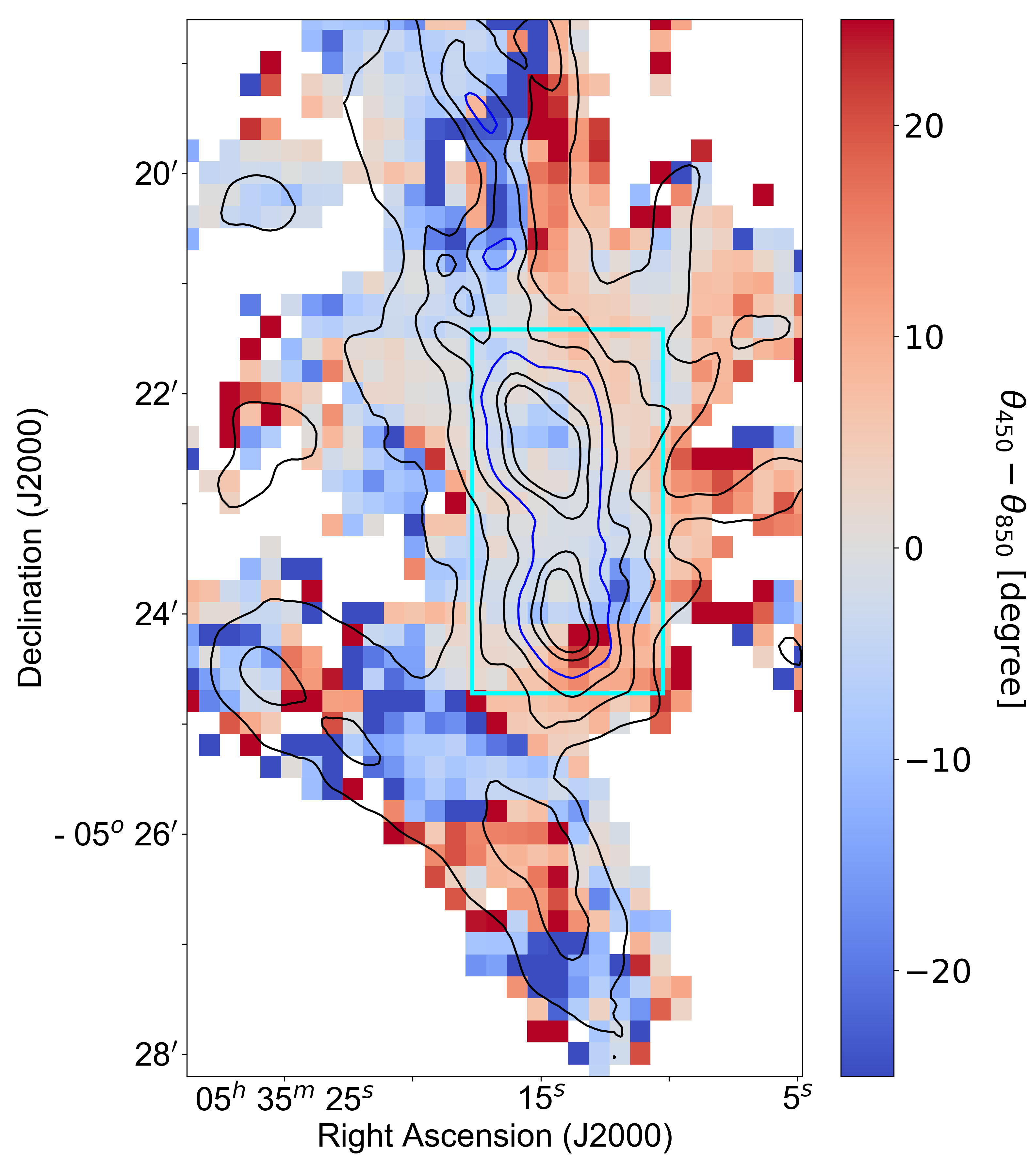
Figure 13 shows the map of differences of angle dispersions at 450 m () and 850 m (). The maps of angle dispersions at two wavelengths are shown in Figure 4. The mean and standard deviation values of the differences are -0.3 degrees and 1.1 degrees. Most of angle dispersions at two wavelengths are similar within 2 degrees which is smaller than the mean measurement uncertainties of polarization segments at 450 m and 850 m.

Appendix B Angle dispersion using a small moving box

We explain the detailed processes to estimate the angle dispersion by which we manipulate our polarization data to obtain the mean field distribution in OMC-1 using a box containing 25 pixels. Figure 14 shows a cartoon of our method. The moving box is represented by a 55 pixel box (in pink) and each pixel contains a model magnetic field segment (e.g., a polarization segment rotated by 90 degrees). We calculate a mean polarization angle, in the box, where and are the mean values averaged over the box. The obtained mean polarization angle is assigned to the central pixel of the box. We repeat the calculation of the mean polarization angle by moving the box over the whole OMC-1 region by one pixel at a time. After obtaining the map of mean polarization angles in the OMC-1 region, we calculate the angle difference between each original segment and the mean polarization angle at the position, i.e. , at pixel (, ). Due to the 180-degree ambiguity of the polarization angle, we take the angle between the original and the mean polarization segments to be less than 90 degree by assuming that the magnetic field orientations do not dramatically change in the small box, 40. We exclude polarization segments if their directions make significant changes in the box based on radii of curvature of the segments (see Appendix C). Since we know an angle difference at every pixel of the OMC-1 region, we calculate an angle dispersion in the box as the root mean squared of the angle differences in 25 pixels, . The angle dispersion obtained is assigned to the central pixel of the box. By moving the box one pixel at a time and calculating the angle dispersion in the box over the whole OMC-1 region, we derive an angle dispersion map of the region.
Appendix C Curvature of magnetic field lines
It is necessary for us to justify which box size is appropriate to estimate the angle dispersion in the OMC-1 region, so we examine the relation between box size and radius of curvature of magnetic field lines described by polarization segments. We calculate the change of angle dispersion by increasing the radius of curvature for three different box sizes in a very idealized set of concentric circular magnetic field lines. The concentric circles, with a common origin at (0,0) in the () plane, are shown as black lines in the left panel of Figure 15. A radius of curvature at an () position is the same as the radius of a circle which passes through the () point. A tangent line of the circle at that position is expressed as a red segment in the figure. The slope of the line is expressed as an angle. The blue lines show a 33 pixel box. We calculate a mean angle of nine slopes in the box and assign the mean angle to the center pixel of the box. After determining mean angles in the nine pixels by moving the box vertically, horizontally and diagonally by one pixel, we estimate the angle difference between the mean angle and the original angle of a slope at each pixel. We then take the root mean squared of the nine angle differences as the angle dispersion in the box and assign the angle dispersion to the central pixel of the box. We calculate angle dispersions by moving the center pixel of a box along the -axis from one-pixel distance from the origin to 100-pixel distance. These processes are also taken in the observational analysis to estimate the distribution of angle dispersion (see section III.1). We repeat the previous processes over the same concentric circular field lines for 55 and 77 pixel boxes to estimate angle dispersions as a function of the ratio of the radius of curvature to the box size ().
The right panel of Figure 15 shows estimated angle dispersions as a function of using three different boxes in units of pixels. The angle dispersion decreases as a function of . When the ratio is infinite such as when the box size is very much smaller than the radius of curvature (/ 1), the angle dispersion should approach zero. Indeed, when the box size is smaller than the radius of curvature (), the angle dispersion is quite well estimated. As the box size approaches the radius of curvature (e.g., ), the angle dispersion increases rapidly. For example, at , the angle dispersion is 0.1 degrees, whereas at , the angle dispersion is a factor of five higher at 0.5 degrees.


In our polarization map of the OMC-1 region, we calculate a radius of curvature at every measured point. A radius of curvature can be estimated by drawing a circle that goes through the two adjacent pixel points at which the two segments become tangent lines to the circle. The curvature radius will be increased when two polarization segments have similar directions. Koch et al. 2012 estimated the curvature of a magnetic field line that goes through two neighboring polarization segments using the following formula:
| (C1) |
where is the curvature, is the radius of curvature, is the distance between two neighboring segments and is the difference of polarization angles at two adjacent pixels. Four pairs of polarization segments are available at a pixel with its left, right, up and down pixels. The mean value of the four radii of curvature obtained from the pairs is assigned to the pixel.
By applying this measurement of the radius of curvature at every point, we obtain radius of curvature maps of the OMC-1 region at 450 m and 850 m in units of arcseconds (Figure 16). The pixels outlined in gray have radii of curvature 40′′, which is the same as a side of a 55 pixel box. All radii of curvature except those in gray pixels inside the lowest contour level are larger than the box size. A 33 pixel box also can be used to estimate angle dispersion in the OMC-1 region, but the box contains only nine pixels. It is not enough to estimate mean angle and angle dispersion. Also, a side of the box is 24′′ which is only about 1.6 times larger than the JCMT beam size at 850 m. It only contains less than three beams. Therefore, we choose the 55 pixel box to measure angle dispersion and magnetic field strength distribution in the OMC-1 region.