© 2021 IEEE. Personal use of this material is permitted. Permission from IEEE must be obtained for all other uses, in any current or future media, including reprinting/republishing this material for advertising or promotional purposes, creating new collective works, for resale or redistribution to servers or lists, or reuse of any copyrighted component of this work in other works.
Fast Synthesis for Symbolic Self-triggered Control under Specifications
Abstract
We extend previous work on symbolic self-triggered control for non-deterministic continuous-time nonlinear systems without stability assumptions to a larger class of specifications. Our goal is to synthesise a controller for two objectives: the first one is modelled as a right-recursive LTL formula, and the second one is to ensure that the average communication rate between the controller and the system stays below a given threshold. We translate the control problem to solving a mean-payoff parity game played on a discrete graph. Apart from extending the class of specifications, we propose a heuristic method to shorten the computation time. Finally, we illustrate our results on the example of a navigating nonholonomic robot with several specifications.
I Introduction
Self-triggered control has been increasingly attracting attention from academia and has proven to be a practical control approach, especially for networked control systems [1, 2, 3, 4]. Unlike conventional periodic control schemes, self-triggered control is a proactive control paradigm with a triggering mechanism that prescribes a time when the control signal has to be updated. As sensing and actuation are performed only when needed, this control scheme can reduce energy consumption and communications across the network. Self-triggered controllers can significantly reduce the communications in nonholonomic robots formation control [3] and the energy consumption in leader-follower consensus control of networked multi-agent systems [4].
However, previous self-triggered control studies focus on stability [1, 5], consensus [4], and reachability or safety [2] problems. To extend self-triggered control to complex specifications such as temporal logic, we consider symbolic control, which is an abstraction-based control approach that constructs a discrete abstraction of the continuous system, then synthesises a discrete controller that can be refined to a controller for the original system in a sound way [6, 7, 8, 9, 10]. Using this technique, we can apply the algorithms developed for discrete structures, such as games on graphs, to synthesise provably-correct controllers for complex specifications that can hardly be enforced with conventional control methods.
The first symbolic self-triggered control approach was introduced in [2] for discrete-time deterministic nonlinear systems under reach-avoid specifications. It was developed in the symbolic control framework for nonlinear systems without stability assumptions proposed in [6]. Our previous work in [11] extended the concept in [2] to the control of continuous-time non-deterministic nonlinear systems for 2-LTL specifications: a subclass of Linear Temporal Logic (LTL) specifications strictly more expressive than reach-avoid. Our control objective was to: 1) control the system to satisfy the given 2-LTL formula and 2) restrict the limit average control-signal length to stay above a given threshold. We reduced the control problem to solving a winning strategy in a mean-payoff parity game played between the controller and the environment. Then, we transformed the winning strategy into a symbolic self-triggered controller of the original system.
In this work, we extend our self-triggered control methodology proposed in [11] to specifications. We add the temporal operator Until, which is a basic operator in LTL but must be treated differently from the other operators in 2-LTL. Dealing with Until heavily increases non-determinism in the mean-payoff parity game. Moreover, unlike previous self-triggered control studies that considered constant control signals of different lengths in a sample-and-hold manner [1, 2], we consider piecewise-constant control signals, resulting in a far larger set of signals choices. For these reasons, we develop a heuristic pruning method to speed up the computation. It disables some control signals based on a notion of reward for execution traces in a Büchi automaton corresponding to the formula. We use the proposed heuristic and reachability analysis, which significantly reduces the computation time.
We study a self-triggered control problem for non-deterministic continuous-time nonlinear systems without stability assumptions, so the system runs in continuous time (even though the controller only sees the discrete sequence of states at the end of input signals), so approaches with discrete-time semantics, such as [9] cannot be applied. Our approach under-approximates the set of atomic propositions that hold along the system trajectories, which is different from [7] that considers state abstraction with robust margin. Moreover, since specifications are strictly more expressive than safety and reach-avoid, we cannot use feedback- or counterexample-based abstraction refinement techniques developed for those specifications, such as in [8].
Our controller synthesis process is a refinement of the one we defined in [11] (see Fig. 1). The main steps of the process (in black in Fig. 1) is to discretise the continuous system into a symbolic model , which is then turned into a mean-payoff parity game . We then compute a winning strategy for , which can be turned into a controller for , and ultimately for . Since there is currently no algorithm to compute winning strategies efficiently, we introduce two intermediate steps (in red in Fig. 1) to reduce the size of the game. The first one is a heuristic that prunes some transitions of the symbolic model, and the second one precomputes the reachable part of the game before solving it.
Notation: For a vector , we write for its infinity norm . Given and , we write for the ball of centre and radius . Finally, given a set , we denote its powerset by .
II Control Framework
II-A Non-deterministic Continuous-time Nonlinear System
We consider a system modelled by a 6-tuple
where and are bounded convex spaces respectively of states and control inputs, is a set of initial states, is a set of control signals of the form that assign a control input at all time in with , and , are forward and backward dynamic functions such that . We denote by the length of signal . The dynamics are defined on , but we are only interested in the bounded subspace .
As in [11], we require the following assumptions, which basically ensure that we can bound the distance between points evolving according to the system dynamics. Note that this does not imply any stability assumptions on .
Assumption 1.
The system is incrementally forward and backward complete. Namely, and for all and and, for all , there are functions such that: 1) for all , and are increasing, and 2) for all , , and ,
- •
- •
Assumption 2.
For all , there are functions such that 1) for all , and are increasing, and 2) for all and , we have
- •
- •
Definition 1.
A run (resp. finite run) of is a sequence (resp. ) such that, for all (resp. ), 1) , 2) , and 3) for all . Let (resp. ) denote the set of all runs (resp. finite runs) of .
We need runs of a system to be discrete sequences of states, since controllers will only observe the state of the system when outputting a signal, but the system runs in continuous time. To match discrete runs to continuous sequences of states, we introduce the notion of trajectory.
Definition 2.
A trajectory of a system induced by a run is a function such that, for all and all ,
Let be the set of trajectories of that are induced by a run . For any finite run , is the set of finite trajectories defined in the same way. Let .
II-B Controlled System
In this section, we define controllers and controlled systems, and explain the self-triggered control process.
Definition 3.
A controller of is a function .
Technically, a controller is a partial function that only needs to be defined on the runs it will generate, but we keep this definition for simplicity.
Let denote the system controlled under the controller . A run (resp. a finite run ) is generated by if, for all (resp. ), . Let (resp. ) denote the set of all runs (resp. finite runs) generated by from any . The definitions of trajectories and carry over to controlled systems directly.
Notice that a controller of a system is defined based on its runs, rather than its trajectories. This is because the controller issues control signals based on runs, which only track the states at the end of each signal.
The overview of the control process is illustrated in Fig 2. First, the controller observes the initial state and issues control signal . Then, to reduce the communication rate, the controller is inactive throughout the duration of . The longer is, the less communication is sent across the network. Since the system is non-deterministic, there are several states that can possibly be reached under the signal . When the signal ends, the controller becomes active and resolves the non-determinism by detecting the actual current state and issue a new control signal . The process is then repeated.
III Problem Formulation
Our goal is to synthesise a controller that satisfies two objectives. The first one is a temporal specification, described as a formula. The second one is a communication rate objective, ensuring that the average length of the issued control signals is above a given threshold.
III-A Right-recursive LTL Specification
We model the first objective using a fragment of LTL, which we call , and which is also an extension of 2-LTL, studied in [11]. Let denote the set of atomic propositions, i.e., assertions that can be either true or false at each state . Let assign the set of atomic propositions that hold at each state.
Definition 4.
Let be the logic whose formulas are the ’s generated by the following grammar:
where is an atomic proposition.
We call ’s state formulas and ’s path formulas. A logic specification is written as a path formula. Here, , , and are given the usual LTL semantics. A state satisfying a state formula is denoted by . We use the same notation for a trajectory and a path formula . For all , is defined as follows:
and for all , is defined as follows:
III-B Controller Synthesis Problem
Definition 5.
Given a system , a set of atomic propositions, a function , a formula , and a threshold , the controller synthesis problem is to synthesise a controller such that
- •
all finite runs in can be extended to an infinite run in ,
- •
for any , and
- •
for any .
The first condition simply ensures that the controlled system will not reach a deadlock, while the other two are the actual control objectives.
IV Problem Reduction to Mean-payoff Parity Games
IV-A Reduction to Symbolic Control
In this section, we state our symbolic controller synthesis problem, which considers a discrete system obtained by quantising states and inputs, and by restricting control signals to piecewise-constant ones. We show that a symbolic controller for this problem also satisfies the conditions in Definition 5.
A symbolic model is a tuple , where , , and are finite sets respectively of discrete states, initial states, and signals, and is a transition function. The notions of runs and finite runs carry directly to symbolic models. Similarly for controllers, which we call symbolic controllers in this case.
Given a time step , signal length bounds , and a discretisation parameter , let
be a set of piecewise-constant control signals, where
| (1) |
is the input set quantised by -dimensional hypercubes of edge length . Since is bounded, each signal is a concatenation of constant signals of length and value in the finite input set , so is finite.
For a given , let
| (2) |
Definition 6.
The symbolic model of a system for input-space quantisation parameters , , and , and state-space quantisation parameter is
such that if and
- 1.
and , , and
- 2.
,
- 3.
,
Notice that may contain some points that are not in , but they have no outgoing transition in , so they will not influence our controller synthesis algorithm.
Remark 1.
A symbolic controller of can directly be turned into a controller of by , where is the closest point to in .
Definition 7.
Given a system , a set of atomic propositions, a function , a path formula , a threshold , and quantisation parameters , the symbolic controller synthesis problem consists in synthesising a symbolic controller such that
- •
all finite runs in can be extended to an infinite run in ,
- •
for any , and
- •
for any .
Theorem 1 (extended from [11]).
IV-B Atomic Propositions along Symbolic Transitions
We want to recover some information about visited states along trajectories, which is lost in the symbolic model. More precisely, we need to know which atomic propositions hold along trajectories. To this end, we introduce functions that under-approximate these sets. They will be crucial in the problem translation in Section IV-D.
For all transitions in the symbolic model , we require that for ,
| (3) | ||||
The intuition is as follows. If (resp. ), then, along the transition , each holds at all times (resp. at some time) and no holds at any time (resp. each does not hold at some time). Then, we can define inductively on the state formula as usual.
For the implementation, we use functions such that, for all states and radii , and are the sets of atomic propositions that are satisfied and not satisfied, respectively, at all states in the ball . In the latter, we assume that, for all states and radii , and can be computed.
IV-C Mean-payoff Parity Games
We recall some known results about mean-payoff parity games (MPPGs) that we use for solving the symbolic controller synthesis problem. We invite the interested reader to see [15] for more details about MPPGs.
Definition 8.
A mean-payoff parity game is a tuple , where
- •
is a directed bipartite graph. is partitioned into two disjoint sets and of vertices for Player-1 and Player-2, respectively. is its set of edges. Functions and map edges to their sources and targets.
- •
maps each edge to its payoff.
- •
maps each vertex to its colour.
- •
is a given mean-payoff threshold.
A play on is an infinite sequence such that, for all , and . A finite play is a finite sequence in defined similarly. Let be the set of all finite plays, and and be the set of those ending with a vertex in and , respectively. Both players play according to strategies. A strategy of Player- is a partial function such that , i.e., chooses an edge whose source is the ending vertex of the play if such an edge exists, and is undefined otherwise. A play is consistent with if for all . For an initial vertex and strategies and for both players, we denote by the unique play consistent with both and . This play may be finite if a player cannot choose an edge.
For an infinite play , we denote the maximal colour that appears infinitely often in the sequence by . The mean-payoff value of is . A vertex is winning for Player-1 if there exists a strategy of Player-1 such that, for any strategy of Player-2, is infinite, is even and . Such a is called a winning strategy for Player-1 from the vertex . The threshold problem [16] is to compute the set of winning vertices of Player-1 for a given MPPG.
In [16], the authors propose a pseudo-quasi-polynomial algorithm that solves the threshold problem and computes a winning strategy for Player-1 from each winning state. In Section IV-D, we reduce the symbolic control problem to the synthesis of a winning strategy on an MPPG, which can be solved using this algorithm.
IV-D Problem Translation to Mean-payoff Parity Games
We translate the control problem for a formula and a threshold to finding a winning strategy for a mean-payoff parity game . All the constructions are given in [11] except for Until, so we only give intuitions here.
Let us start with the construction of the base game, illustrated in Fig. 3. There, Player-1 corresponds to the controller, and Player-2 to the environment. Each discrete state is mapped to a Player-1 vertex, and each pair is mapped to a Player-2 vertex. Each has an edge to , which corresponds to the controller sending control signal . Each has an edge to if , which corresponds to resolving the environmental non-determinism. All such edges have payoff , and the colouring of states is undefined (it is defined later by induction on the formula).
Let us consider the discrete system in Fig. 4, which has a single input signal , so we omit it for readability. The constructions of and are given in Fig. 5 (the other cases are similar). Each of them contains two copies (coloured green and red in Fig. 5) of the base game. Colours are constant on each copy, and given by the coloured numbers in Fig. 5. Edges from to always stay in the same copy, while edges from to may switch to a different copy (in Fig. 5, arrows from are coloured with the colour of the copy they point to). For , an edge from the first copy points to the second one if , and edges from the second copy always point there; the intuition is that the second copy is a losing copy for Player-1, and we should move to it if at some point it cannot be shown that holds all the time along the transition. For , an edge points to the second copy if and to the first one otherwise (independently of the starting copy); the intuition being that the second copy detects points where it can be shown that holds at some point along the transition, and it needs to be visited infinitely often to win the game.
where stands for
and similarly for .
We now explain the new case, namely the Until case. A graphical description of the construction of is described in Fig. 6. It contains , which comes equipped with an initial copy of the base game (for example, in the games of Fig. 5, is the green copy). It also contains a new copy of the base game. The intuition is that this new copy will be used to encode the verification of the part of , while will be used for . This new copy of the base game is different from the one shown in Fig. 3 on two aspects. First, there are two Player-2 nodes for each pair : edges from the first one stay in the new copy, while edges from the second one go to . This corresponds to Player-1 making a choice whether to keep checking or to start checking . Second, there are edges from to a only if for all . This is because must hold at all times regardless of system non-determinism in the first part of specification . In Fig. 6, the dashed edges from do not exist in the game, because one of the non-deterministic branches does not verify the condition above.
Building and basically corresponds to synchronising parity automata by remembering, for each colour of the first automaton the largest colour seen in the other since the last time was seen during the current execution. If or is an Until formula, the construction can be optimised to avoid state space explosion: one only needs to start remembering colours when both automata have finished checking the first part of the Until.
Theorem 2 (extended from [11]).
From a winning strategy for Player-1 in , one can effectively compute a symbolic controller for that solves the symbolic controller synthesis problem of Definition 7.
The proof is an obvious extension of that in [11].
V Controller Synthesis Algorithm
V-A Algorithm Overview
The overview of our process is illustrated in Fig. 1. First, we discretise the system into the symbolic model based on the quantisation parameters , , , and . Then, using the heuristic pruning algorithm proposed in Section V-B, we disable the control signals that do not look promising to verify . We transform the pruned symbolic model into a mean-payoff parity game, as discussed in Section IV. Then, we reduce the size of the mean-payoff parity game by removing the vertices that are not reachable from the initial state. After solving the mean-payoff parity game, if there exists a winning strategy for Player-1, we translate it to a symbolic controller. If the algorithm fails to compute a winning strategy, we may refine the quantisation parameters (e.g., setting , or , or ) and repeat the process until the parameters become smaller than a predefined threshold.
A challenge faced in practice with discretisation is that the generated systems and games are too large to solve for larger state spaces. We present both the heuristic pruning algorithm and the reachability computation in the following subsections, and demonstrate their effectiveness using the experimental results in Section VI.
V-B Heuristic Pruning


We develop a heuristic pruning algorithm to only keep the control signals that look most promising to verify . For simplicity, we only describe the algorithm on a symbolic model with a single initial state . We first translate into its corresponding Büchi automaton , which can be done using tools such as Spot [17]. Some examples of this translation are shown in Fig. 7. Then, we assign a reward to each Büchi state using a function , where is ’s set of states, following the principles below. For each accepting state we assign , which is the highest possible reward. For each from which it is impossible to reach any accepting state (e.g., state in Fig. 7(b)), we assign . Otherwise, we may choose the reward to be any value in . For the example in Fig. 7 (a), we assign reward 0.5 to the states and , as they correspond to the case where one of the atomic proposition ( or ) is detected.
Then, we monitor finite runs of length at most in the synchronised product from its initial state , based on which we disable some control signals. More precisely, we build a tree whose nodes are either in or in , of depth as in Fig. 8. For each node at depth of the tree, we compute the estimated reward of as follows.
| (4) |
and .
In words, is the maximum reward that the controller can ensure to see in for runs of length at most . If , it means the system can be controlled to go through an accepting state. Red nodes in Fig. 8 represent the non-determinism of the system, which can go to any reached by , so has to be defined as a minimum of their expected rewards.
We prune the symbolic model at state by disabling signals that do not maximise . We also remove a state from if all control signals are disabled at .
Notice that each pair may appear multiple times in the tree in Fig. 8 (e.g., if there is a cyclic run). To save computation time, we avoid computing if is detected at depth and the value has already been previously computed at depth . As a result, our pruning algorithm is non-deterministic, depending on which branch of the tree we compute first. Also note that our pruning algorithm disables the signals for discrete states, which correspond to several vertices in . Thus, there is a possibility that the algorithm prunes control signals that are needed for the controller to win.
Note that, in general, there are more than one initial state in , in which case the algorithm extends directly using a forest rather than a tree.
Remark 3.
Since the pruning process only prunes signals (and not the non-determinism), it only constrains the system, so a controller that solves the problem in Definition 7 for the pruned system also does it for the whole system.
V-C Reachable Subgame
We compute the reachable subgame of from initial vertices in a breadth-first traversal manner, where is the set of initial states that belong to the initial copy of . More precisely, we first set , and repeatedly compute the set of reachable vertices from after exactly transitions. Concretely, we compute as the set until for some . Then, we apply a mean-payoff parity game solver on the subgame that contains the reachable vertices, i.e., . Fig. 9 shows an example of computation of the reachable subgraph. Observe that according to the definition, each vertex is visited at most once.
This technique may look simple, but it is already very efficient. Indeed, as we will see in Section VI, this removes a large number of vertices. Actually, this allows to remove entire copies (as described in Section IV-D) in the game.
Remark 4.
Because the existence of a winning strategy is only affected by the reachable part of the game, each winning strategy on the reachable subgame is also a winning strategy on the whole game.
VI Experimental Results
| no | prune | no | prune | |||
| spec. | pre- | reach | + | pre- | reach | + |
| comp. | reach | comp. | reach | |||
| loop | 202 | 36 | 33 | 82272 | 12866 | 4920 |
| 2-loop | 16131 | 853 | 157 | 658176 | 33780 | 4497 |
| until-1 | timeout | 2351 | 211∗ | 709506 | 35107 | 12853 |
| until-2 | timeout | timeout | 964 | 1181964 | 69744 | 39339 |
As in [11], we consider a non-deterministic nonholonomic robot system. This is a modified version of [3], to allow non-determinism, coming from uncertainties in the measure of the velocity.
In this system, the input signal is given by , the steering angle. The physical dimensions are , , and , respectively the cartesian coordinates and heading angle. The speed of the robot is . The non-determinism is given by , randomly chosen from for .
Functions and , as well as their backward versions, can easily be computed (more details are given in [11]). We use our controller synthesis algorithm with the following parameters: , , , , , , , , and . The state space depends on the specification. For the mean-payoff specification, we set the threshold , meaning that at least half of the input signals must be of length .
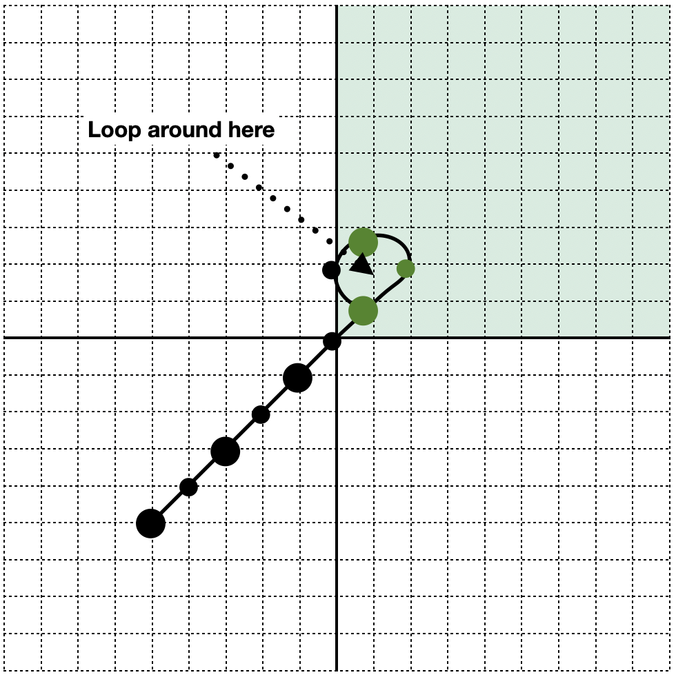
We consider the four specifications depicted in Fig. 10. The loop specification (Fig. 10(a)) is given by the right-recursive LTL formula , where green stands for the atomic proposition . This means that the robot must visit the green area infinitely often. The 2-loop specification (Fig. 10(b)) is given by , where blue stands for , and red for . In this case, the robot must navigate infinitely often between the upper and the lower parts of the state space. The until-1 specification (Fig. 10(c)) is given by , where blue is , red is and green is . Here, the robot must stay in the left side of the state space until it reaches and stays forever in the upper part, and it must visit the right side infinitely often. These three specifications share the same state space . Finally, the until-2 specification (Fig. 10(d)) is the same as until-1, except that blue stands for , green for and the state space is larger . Notice the increasing complexity in the specifications: 2-loop is more complex than loop, until-1 than 2-loop, and the state space of until-2 is larger than that of until-1.
To solve the mean-payoff parity game, we combine the reduction of mean-payoff parity games to energy games in [18] with the solver for energy games in [19]. The program was implemented in Python 3.8.6 and run on a MacBook Pro (Apple M1 chip, 16GB memory). The results are compiled in Tab. I. For each specification, we ran our algorithm without any precomputation, with reachability only, and with both reachability and heuristic pruning. The times given for the cases using pruning are averaged over executions, as this heuristic is non-deterministic. The system studied in [11] is the loop specification without any precomputation.
We observe that precomputations decrease both the size of the game, and the execution time. The algorithm without precomputation easily reaches timeout (set at hours) when the specification becomes more complex. For 2-loop and until-2, we observe that pruning makes the execution significantly faster, compared to reachability only. For until-2, reachability only is not even enough to avoid a timeout. There are two main reasons: first the size of the game is much larger; second, there are many more non-winning states for the mean-payoff specification, which makes the energy game solver (which uses value iteration) much slower.
Finally, the third specification until-1 witnesses the limitations of pruning (already mentioned in Section V-B): by pruning, we may remove some winning strategies. In this particular case, we remove all of them. However, because our algorithm reaches this conclusion faster than with reachability only, there is little harm in pruning.


VII Conclusion and Future Work
We proposed a symbolic self-triggered controller synthesis algorithm for non-deterministic continuous-time nonlinear systems without stability assumptions under two control specifications: a specification and a threshold for the average control signal length. The main steps of the process are 1) to discretise the state and input spaces to obtain a symbolic model corresponding to the original continuous system 2) to reduce the controller synthesis problem to the computation of a winning strategy in a mean-payoff parity game. In addition, we proposed a heuristic pruning algorithm to speed up the computation by disabling some control signals based on expected rewards in a Büchi automaton generated from the specification. We demonstrated the efficiency of our method on the example of a nonholonomic robot navigating in an arena under several specifications.
For future work, we want to further investigate heuristics that help solve games in practice by trying different variants and tradeoffs for our pruning algorithm. One possibility would be to prune the game – rather than the symbolic model, which would be harder but would also retain more strategies and could be done while computing the reachable set. Another would be to prune from different states – rather than only from the initial states – and see if it can improve performance. Another direction is to explore different reward strategies for the Büchi automata used by the heuristic. Moreover, we want to develop a theory of Büchi automata with structured alphabets that is suitable for our use.
References
- [1] W. P. M. H. Heemels, K. H. Johansson, and P. Tabuada, “An introduction to event-triggered and self-triggered control,” in Proc. 51st IEEE Conf. on Decis. and Control, 2012, pp. 3270–3285.
- [2] K. Hashimoto, A. Saoud, M. Kishida, T. Ushio, and D. V. Dimarogonas, “A Symbolic Approach to the Self-Triggered Design for Networked Control Systems,” IEEE Contr. Syst. Lett., vol. 3, no. 4, pp. 1050–1055, 2019.
- [3] C. Santos, F. Espinosa, M. Martinez-Rey, D. Gualda, and C. Losada, “Self-Triggered Formation Control of Nonholonomic Robots,” Sensors, vol. 19, no. 12, pp. 132–139, 2019.
- [4] J. Liu, Y. Zhang, Y. Yu, and C. Sun, “Fixed-Time Leader-Follower Consensus of Networked Nonlinear Systems via Event/Self-Triggered Control,” IEEE Trans. Neural Netw. Learn. Syst., vol. 31, no. 11, pp. 5029–5037, 2020.
- [5] A. Anta and P. Tabuada, “To Sample or not to Sample: Self-Triggered Control for Nonlinear Systems,” IEEE Trans. Autom. Control, vol. 55, no. 9, pp. 2030–2042, 2010.
- [6] M. Zamani, G. Pola, M. Mazo, and P. Tabuada, “Symbolic Models for Nonlinear Control Systems Without Stability Assumptions,” IEEE Trans. Autom. Control, vol. 57, no. 7, pp. 1804–1809, 2012.
- [7] J. Liu and N. Ozay, “Finite abstractions with robustness margins for temporal logic-based control synthesis,” Nonlinear Anal.: Hybrid Syst., vol. 22, pp. 1–15, 2016.
- [8] K. Hsu, R. Majumdar, K. Mallik, and A. K. Schmuck, “Lazy Abstraction-Based Control for Safety Specifications,” in IEEE Conference on Decision and Control, 2018, pp. 4902–4907.
- [9] L. Lindemann and D. V. Dimarogonas, “Robust Control for Signal Temporal Logic Specifications using Discrete Average Space Robustness,” Automatica, vol. 101, pp. 377–387, 2019.
- [10] E. Macoveiciuc and G. Reissig, “Memory efficient symbolic solution of quantitative reach-avoid problems,” in Proc. Amer. Control Conf., 2019, pp. 1671–1677.
- [11] S. Pruekprasert, C. Eberhart, and J. Dubut, “Symbolic Self-triggered Control of Continuous-time Non-deterministic Systems without Stability Assumptions for 2-LTL Specifications,” in 16th Int. Conf. on Control, Automat., Robot. and Vision, 2020.
- [12] D. Angeli and E. D. Sontag, “Forward completeness, unboundedness observability, and their Lyapunov characterizations,” Syst. and Control Lett., vol. 38, no. 4, pp. 209–217, 1999.
- [13] D. Angeli, “A Lyapunov approach to incremental stability properties,” IEEE Trans. Autom. Control, vol. 47, no. 3, pp. 410–421, 2002.
- [14] K. Hashimoto and D. V. Dimarogonas, “Synthesizing Communication Plans for Reachability and Safety Specifications,” IEEE Trans. Autom. Control, vol. 65, no. 2, pp. 561–576, 2019.
- [15] K. Chatterjee, T. A. Henzinger, and M. Jurdzinski, “Mean-payoff parity games,” in Proc. 20th Annu. IEEE Symp. Log. Comput. Sci., 2005.
- [16] L. Daviaud, M. Jurdziński, and R. Lazić, “A pseudo-quasi-polynomial algorithm for mean-payoff parity games,” in Proc. 33rd Annu. ACM/IEEE Symp. Log. Comput. Sci., 2018, pp. 325–334.
- [17] A. Duret-Lutz, A. Lewkowicz, A. Fauchille, T. Michaud, E. Renault, and L. Xu, “Spot 2.0 — A Framework for LTL and -Automata Manipulation,” in Proc. 14th Int. Symp. Automated Technol. Verification and Anal., ser. Lect. Notes Comput. Sci., vol. 9938. Springer, 2016, pp. 122–129.
- [18] K. Chatterjee and L. Doyen, “Energy parity games,” Theor. Comput. Sci., vol. 458, pp. 49–60, 2012.
- [19] L. Brim, J. Chaloupka, L. Doyen, R. Gentilini, and J.-F. Raskin, “Faster algorithms for mean-payoff games,” Form. Method. Syst. Des., vol. 38, no. 2, pp. 97–118, 2010.