Two-Stage Monte Carlo Denoising with Adaptive Sampling and Kernel Pool
Abstract
Monte Carlo path tracer renders noisy image sequences at low sampling counts. Although great progress has been made on denoising such sequences, existing methods still suffer from spatial and temporary artifacts. In this paper, we tackle the problems in Monte Carlo rendering by proposing a two-stage denoiser based on the adaptive sampling strategy. In the first stage, concurrent to adjusting samples per pixel (spp) on-the-fly, we reuse the computations to generate extra denoising kernels applying on the adaptively rendered image. Rather than a direct prediction of pixel-wise kernels, we save the overhead complexity by interpolating such kernels from a public kernel pool, which can be dynamically updated to fit input signals. In the second stage, we design the position-aware pooling and semantic alignment operators to improve spatial-temporal stability. Our method was first benchmarked on 10 synthesized scenes rendered from the Mitsuba renderer and then validated on 3 additional scenes rendered from our self-built RTX based renderer. Our method outperforms state-of-the-art counterparts in terms of both numerical error and visual quality.
1 Introduction
Restoring degraded visual signals with noise is of immense importance to the computer vision and graphics community. With the recent success of deep learning algorithms, great progress has been made on denoising images [24, 34] and videos [38, 31, 6]. As one of the most common degradation types in digital images, injected Gaussian noise [21], can be regarded as stochastic samples in a latent Gaussian distribution and can be easily captured by well-designed convolutional neural networks. However, capturing videos under low intensity light circumstances usually introduce realistic noise with more complex implicit patterns. A naive apply of standard Gaussian noise removal methods on such realistic noise will not suffice [35, 36, 37].
As a simulation of real-world light transmission, ray tracing introduces a large amount of realistic noise when the light sampling count is limited. Current Monte Carlo path tracers randomly sample lighting directions on hemispheres modeled on the collision of scene objects with the emitted lights, makes the decision of lighting path from the light source to the observer a fully stochastic process. When the number of samples per pixel (spp) is considerably low, scarce lighting information causes a great amount of realistic noise. Therefore, a pertinent denoiser to this specific situation is desired to handle the unstructured noise and smooth the significant degradation in the rendered scenes.
Recent advances on denoising path traced videos depend on recurrent variants [33, 5, 15] of U-Net [25] that are fed with video frames iteratively to capture better temporal information. Despite the careful handling of temporal disparities [1, 4, 18], denoised frames still suffer from loss of reconstruction details, especially at dark regions and object contours. Reconstruction failures are blamed on the insufficient visual clues provided in the raw rendered image where lights are hard to reach or transmit through. Monte Carlo path tracing at interactive sampling rates [17, 9] serves as a good remedy to such problems. Instead of sampling light rays uniformly, the ray number per pixel is dynamically determined through an additional neural network. Although such adaptive sampling methods perform well on hard-to-denoise pixels, there are two major flaws: (1) As a trade-off to the increasing performance, overall computational costs inevitably doubled due to the introduction of a second network. (2) Distributing a limited sampling budget to all frame pixels undermines the visual quality at low-frequency regions, and consequently harms spatial stability.
In this work, our three-fold contributions are made to overcome the above flaws. (1) We rethink the adaptive sampling framework by reusing the computations in the sampling network to function as an initial denoising process. Apart from the determination of sampling count per pixel, we learn an affiliate set of denoising kernels to achieve an initial denoising. Differing from existing Kernel Prediction (KP) [33, 9] methods that spawn one-to-one kernel for each pixel, we minimize the exceeding computation overhead by maintaining a public kernel pool with a fixed number of communal kernels. A pixel-wise kernel map is then produced from the sampling network to guide the interpolation of pixel-wise kernels in the kernel pool. (2) We propose an adaptive pooling scheme, namely position-aware pooling to smooth spatial instabilities by taking positional information into consideration. Additionally, instead of aligning motions for better temporal stability, we introduce semantic alignment that learns feature-wise alignment between the current and precedent frame. (3) Our method was validated on 10 different scenes rendered from the Mitsuba path tracer [11] and 3 additional scenes rendered from our self-built RTX-based renderer. Our method surpasses other counterparts both quantitatively and qualitatively.
2 Related Works
2.1 Denoising for Monte Carlo Rendering
Denoiser for Monte Carlo path tracer enables the renderer to operate in a low sampling count environment without an apparent loss on image quality, saving rendering costs. Here, we focus on reviewing the denoising methods that reconstruct degraded visual signals in the image-space.
Image-space algorithms manipulate discordant color units and reconstruct noisy pixels directly. Starting from utilizing a set of pre-defined filters [14, 27] to work as a weighted linear combination of the noisy pixels at local windows, similar approaches have been experimented with bilateral filters [28, 29] and non-local patches [20]. Instead of combining pixels directly, efforts have been made on generating pixel residuals based on local regressors [3, 19]. The above techniques usually require heavy manual analysis of statistical estimations between the denoised image and reference. The image quality improvement brought by such methods is limited and manually tuned parameters on one scene can hardly generalize to others.
With the thrive of deep learning, neural network based denoisers have been recently more favored. A pioneer practice [13] utilizes a basic multi-layer network to take image-space features as input and predict the parameters for denoising bilateral filters. To smooth the temporal artifacts in a sequence of noisy rendered images, [5] designed a recurrent neural network that denoises rendered video frames based on the iterative forward of the network. However, the disparity between adjacent frames impacts the performance of the recurrent denoiser greatly, and complex image-space motion alignments are desired. Our proposed method follows a similar recurrent paradigm but handles both spatial and temporal instabilities from novel perspectives.
2.2 Adaptive sampling methods
An alternative strategy to alleviate denoising difficulties is to adjust pixel-wise sampling counts dynamically, promoting the renderer to generate more samples on the hard-to-denoise regions and fewer samples to the easier ones.
Early attempts distribute samples adaptively based on the measured errors between the noisy and the reconstructed image pair [7, 22]. The same strategy has also been adopted in [33], however, instead of calculating errors directly, the error map is obtained as the prediction of a neural network. Spp is then iteratively decided in an offline manner. For better adaptation into online rendering, [17] utilizes an additional network to predict sampling map beforehand, based on an initially rendered 1spp image, and then consume the estimated sampling map in the major rendering process. Both networks can be optimized jointly using the final reconstruction loss. In a recent work, [9] handles the temporal artifacts in videos by warping the previously reconstructed frame to initiate current frame denoising. The denoiser is further studied to predict hierarchical denoising kernels at multi-scales. However, the above framework highly depends on motion alignments which can be easily influenced by off-screen pixels and object occlusions. In this work, we reuse computations in the sampling network to serve as a two-stage denoising framework, and design Novel modules to efficiently acquire large receptive fields and smooth spatial-temporal instabilities.
3 Preliminary
Consider a Monte Carlo path tracer rendered noisy image with uniform spp of and a corresponding set of Geometry Buffers (GBuffers) consists of scene depth, shading normal, and albedo at primary hit position. The conventional adaptive sampling framework [9, 17] takes as input , and eventually outputs the denoised image .
The framework is comprised of two networks including a sampling network and a denoising network , both share the same architecture. The sampling network aims at generating a sampling map before the main rendering process initiates. To obtain the valid integer sampling map from the predicted floating values, a simple normalization scheme is followed as suggested in [17]:
| (1) |
where is the total number of pixels and is the expected average spp budget. is then fed into the Monte Carlo path tracer acquiring the adaptively sampled image . However, the involvement of renderer at each iteration of network training is empirically inefficient. To accelerate network training, the rendering process is simulated by pre-rendering a set of images at different uniform spp [17] and assemble the simulated via:
| (2) |
where is an indication function that returns 1 if the binary encoding of is activated at the term. After simulating from , the gradients for is calculated with the help of the ground truth image rendered at high spp: . Note that here is only used for gradient approximation. Both and are then combined to be fed into the denoising network which directly predicts the denoised image .
4 Methods
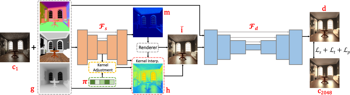
Our proposed framework follows the conventional adaptive sampling paradigm that entails a sampling network followed by a denoising network . Both of the networks are constructed in the U-Net [25] style, such that encoded embeddings at each level are skipped to the decoder for better feature aggregation and gradient preserving. Differing from [17, 9] that and share the identical network architecture, we put less computation resources on and focus more on with deeper encoding depth and larger feature width. Unless explicitly specified, the basic building block is designed as the stack of a 3x3 convolutional layer followed by a ReLU non-linearity layer. An overview of the proposed framework is shown in Figure 2.
4.1 Two-stage denoising with kernel pool
In the existing adaptive sampling paradigm, contributes little to the final denoising quality except for the generation of . However, compared to using as a one-stage denoiser, introducing an extra network inevitably doubles the overall computational costs and slows down the denoising efficiency. We rethink the responsibility of and refactor the network to carry out an initial denoising process on before being fed into . Since the simulation of depends on the prediction of , , therefore, needs to make an inference beforehand. As a result, promoting as a naive regresser similar to is impractical.
Parallel to , we enable the sampling network to generate a set of denoising kernels that is subsequently applied on , obtaining the initially denoised image . However, the commonly adopted pixel-wise kernel prediction method [33] poses a huge challenge to our : with the same backbone network, the prediction of pixel-wise kernels strongly couples with the prediction of , thus easily leads to degradation of identical values across all pixels on either sampling map or predicted kernels. Also, large kernels (21x21 in [33]) are usually too expensive to be predicted, which puts exceeding computation burdens on .
To overcome the above challenges, instead of a direct prediction of pixel-wise kernels, we learn a public kernel pool consisting of a set of communal kernels with fixed size . The kernel pool can be jointly optimized along with the networks. During network inference, differing from [33] that predicts per pixel kernel , our only outputs an extra kernel map indicating the offset of the most appropriate per pixel kernel in the kernel pool. The initial denoising is achieved through two procedures, namely kernel adjustment and kernel interpolation. Similar to [31], our initial denoising process requires no particular supervision.
Kernel Adjustment. Although the optimized kernel pool fits the training data well, such kernels may generalize poorly on the testing data due to the disparity between training and testing images. Towards better generalization ability and better correspondence to the target image, we learn an auxiliary set of kernel residuals to be applied on . Rather than a simple addition of and , sigmoid gated alpha values are additionally learned to achieve kernel-wise alpha blending. In our experiments, we set , hence both the generation of and the initial denoising process yield only little overhead computations.
Detailedly, an additional branch is extended from the deepest encoded features in at the coarsest scale to perform the kernel adjustment separately. The coarsest features are first adaptively pooled to the desired spatial size which are then excited to through a MLP. For better correlations between adjacent kernels, we apply an extra convolution with five neighboring kernels at a time sliding from the first kernel to the last obtaining the kernel residual . We employ an extensive MLP to learn the kernel-wise scores based on the summation of both and . The adjusted kernel pool for the current input image is then calculated as . The kernel adjustment workflow is outlined in Figure 3.
Kernel Interpolation. Since and can be different, we predict by taking as an additional support. Besides, to make sensible to , adjusted kernels are convoluted to a lower dimension with unit spatial size, such kernel descriptor is then spatially expanded and treated as another support. We concatenate the above two supports with the forwarded finest scale features and to generate through a series of convolutions followed by a Tanh layer at the end.
Per-pixel kernels are grid sampled from with the predicted kernel map . However, we found that the public kernel pool is not able to satisfy the need for all pixels across an image, and some pixels may rely more on rather than to be further denoised. To this end, we predict an extra offset in enabling a 2D interpolation between the softmax gated sampled kernel and an identity kernel, which has the same spatial size but is filled with at the center and elsewhere. The updated 2D interpolation enables each pixel in to be flexibly switched between the initially denoised pixel and the raw adaptively sampled pixel.
4.2 Spatial-temporal instability smoothing
Fast GhostConv. Towards better distribution of adaptive samples, visual clues implied in are expected to be well explored. However, path traced samples at low spp pixels may deviate significantly from the true distribution. When determining the light transmission direction via the Monte Carlo method, the stochastically sampled single light ray is likely to have a biased reflection and refraction angle. Consequently, the lighting information rendered in one pixel in could be represented better in another far-located pixel. To this end, basic operators of are desired to be designed with larger receptive fields, considering a wide range of pixels at a time thus capturing the deviated ray samples.
We elevate the reception field while further reducing the computational costs by advanced engineering of the Separable Convolution [10] and the Ghost Module [8]. Standard convolutions are first replaced with large-kernel group convolutions to efficiently gather information in a wide range. Different channels in the wide scale features are then communicated through point-wise convolutions. An additional depth-wise convolution is utilized to obtain extra ‘ghost’ features to further widen the receptive field. We denote such efficient operator as Fast GhostConv which replace the basic building blocks in (Figure 5).
Position-aware pooling. Given the fixed total spp budget, assigning more samples to object contours and dark areas results in fewer samples and worse visual quality in low-frequency regions, which occupy most parts of the scenes and could cause conspicuous spatial flickering (Figure 4). We blame such instability on network pooling, where poorly sampled pixels are usually mixed with good ones, and can be hardly discriminate against.
We learn extra one-to-one scale scores for each member by a cheap MLP in the pooling window to achieve an adaptive pooling. All members in a window are first multiplied with the corresponding scale score and are then summed up altogether to be the pooling result. The scale scores in a window are summed up to 1 and can be gated by a softmax function. Empirically, we found that due to the uncertain directions of ray samples, the proposed pooling strategy is sensitive to positional information. Therefore, we make the adaptive pooling operator position-aware by considering both absolute positions in terms of the whole feature map (encoded as gradient values from the left top corner to the right bottom) and relative positions within the current window (encoded as one-hot vectors).

Semantic Alignment. Inter-frame motions lead to unexpected temporal artifacts. Existing temporal stabilizing methods either estimate pixel-wise motion vectors to align frames directly or consume a sequence of continuous frames at a time. However, the pixel alignment method is sensitive to object occlusions, and consuming consecutive frames demands a large number of extra computations. Considering the above drawbacks, instead of aligning motions in the raw RGB space, we achieve the alignment in the semantic space. The frame matching and occlusion handling are therefore delegated to be learned by the network.
Specifically, we design a transformer [32] style module to reason global correspondences between the current and previous frame features through a multihead attention layer followed by a 2D feed forward convolution. The attentive features are preserved for the inference of the next frame. Similar to other vision transformers, we encode positional information following the Cosine-Sine strategy, and add the 2D encodings to the current frame features to serve as query for the multihead attention. The preserved last frame features function as both value and key. The proposed semantic alignment module is placed at the deepest level of for better efficiency. The design details are shown in Figure 5.

Loss functions. Appropriate loss functions also help smooth the instabilities. We adopt simple losses for both spatial and temporal constraints, denoted as and respectively. is determined on and [5, 9], which can be pre-computed as and at current and previous frames.
Apart from the standard constraints, we apply an additional perceptual loss term [12] to supervise networks based on the feature difference between and inferred by a pre-trained VGG-16 network [30]. Gradients are calculated on the weighted combination of the three losses:
| (3) |
where are scale factors applied on each loss. During training, and are only applied on the last frame in a video sequence, while involves last two frames.
5 Experiments
5.1 Experimental setup
Datasets. Our method was first benchmarked on the videos captured from 10 synthesized scenes [2] (Contemporary Bathroom, The Grey & White Room, Bedroom, Country Kitchen, Modern Hall, The Wooden Staircase, Salle De Bain, The White Room, The Breakfast Room, Japanese Classroom) using the Mitsuba renderer [11]. The trained models were then slightly fine-tuned and transferred to validate on 3 new scenes (Warmroom, Diningroom, Livingroom) rendered from our self-built RTX-based renderer. All scenes commonly have more than one light source and abundant environment illumination. We set up a camera to traverse through the scenes and captured videos based on a set of predefined key nodes in the scenes. Camera position and orientation were linear and quaternion interpolated between two adjacent key nodes by a specified frequency. As mentioned in Sec. 3, we pre-rendered 5 color images at each camera position with spp in to simulate rendering of spp images. GBuffers (normal, depth, albedo) are obtained as the rasterization results at the same view. In total, 8 training images in resolution are required to be rendered at each camera location.
| Methods | PSNR | SSIM | MACs | Params |
|---|---|---|---|---|
| U-Net [25] | 31.91 | 86.00 | 316.52 | 0.972 |
| FastDVDnet [31] | 32.07 | 86.02 | 1083.5 | 1.867 |
| RAE [5] | 31.96 | 86.07 | 432.61 | 1.864 |
| DASR [17] | 31.97 | 86.08 | 558.00 | 1.577 |
| NTASAD [9] | 32.13 | 86.46 | 826.11 | 1.578 |
| Ours | 33.39 | 87.65 | 478.22 | 1.285 |
For Mitsuba scenes, we captured one video per scene with 500 frames using the provided camera trajectories in [5]. The first 100 frames and the last 400 frames are split for validation (testing) and training respectively. We further construct non-overlapping video clips with 5 consecutive frames to be fed in each network forward propagation during both training and validation, which results in 800 training clips and 200 validation clips. In testing, instead of using short clips, models are inferred on all 100 consecutive testing frames directly. For generalization experiments, videos were captured in 100 frames.


Implementation details. Adam optimizer [16] was used to train all models starting from an initial learning rate of 3 and CosineAnealing scheduled to 3 in 300 epochs. We randomly cropped patches for training and center cropped patches for validation. After training converges, we retain the model instance at the epoch with the lowest validation loss to test on full-scale frames. Due to a large number of possible training patches, we didn’t use extra data augmentation techniques. We set batch size to 8 for training and 1 for validation and testing. , and are set to 0.8, 0.2 and 0.1 respectively. Perceptual loss was also applied on all competing methods for fair comparison. The kernel pool with and was binarily initialized following Bernoulli distribution. All experiments were implemented in Pytorch [23] and on Tesla V100 GPUs.
Unless explicitly specified, we expect an average spp budget of 4 for inputs and uniform 2048 spp for reference. Following [9], color images (albedo and ) are converted into gray scale as two additional inputs for . During network forward, and requires two independent renderings. For consistent rendering costs, we subtract 1 spp from the expected budget and linearly blend to .
5.2 Results
Mitsuba results. We first present our denoising results on the videos captured in Mitsuba path traced scenes. Figure 6 shows qualitative results on one exemplary frame. In , we observe that the interpolation principle of kernels is based not only on pixel chrom, but also the semantics reasoned in . Regions with the same color can be denoised with very different kernels. As shown in , our framework demonstrates a good ability to collaborate both adaptive sampling and initial denoising by preserving more samples to the hard-to-denoise regions and fewer samples to the easier ones. We compare our sampling map to other adaptive sampling methods’ in Figure 7. Interestingly, our sampling maps significantly differ from [17, 9] which always assign high spp to specific objects (e.g. glass, table). Our adaptive sampling and initial denoising procedure serve as good complements of each other and the produced becomes more comprehensible to . The final denoised images prove that our method is not only able to remove the realistic noise, but is also capable of reconstructing details (e.g. highlight, object geometry).
We further compare our method to the baseline method: U-Net [25]; state-of-the-art videos denoisers: FastDVDnet [31], RAE [5]; and adaptive sampling counterparts: DASR [17], NTASAD [9]. The average quantitative results on the entire 1000 frame testing set are shown in Table 1. Our proposed framework outperforms all competing methods on both metrics greatly. Notably, except for the methods that use simple encoder-decoder structure [25, 5], our dual-network framework demands the least computation costs and parameter counts. Exemplary qualitative comparisons are shown in Figure 8 Top, and more cases are shown in the supplementary material.
| Model | UN | AS | KP | PP | FG | SA | PSNR | SSIM | rMSE | MACs | Params | |
| A | ✓ | 31.92 | 86.00 | 2.51 | 5.58 | 316.52 | 0.972 | |||||
| B | ✓ | ✓ | 32.13 | 86.81 | 2.52 | 5.09 | 464.87 | 1.348 | ||||
| C | ✓ | ✓ | ✓ | 33.11 | 87.31 | 2.27 | 4.03 | 526.05 | 1.471 | |||
| D | ✓ | ✓ | ✓ | ✓ | 33.29 | 87.51 | 2.17 | 3.79 | 526.40 | 1.471 | ||
| E | ✓ | ✓ | ✓ | ✓ | ✓ | 33.34 | 87.56 | 2.18 | 3.70 | 478.54 | 1.324 | |
| F | ✓ | ✓ | ✓ | ✓ | ✓ | ✓ | 33.39 | 87.65 | 2.16 | 3.67 | 478.22 | 1.285 |
| G | ✓ | ✓ | ✓ | ✓ | 33.22 | 87.33 | 2.20 | 3.89 | 478.34 | 1.324 | ||
| H | ✓ | ✓ | ✓ | ✓ | ✓ | 33.19 | 87.36 | 2.22 | 3.90 | 478.02 | 1.284 | |
| I | ✓ | ✓ | ✓ | ✓ | ✓ | 33.15 | 87.40 | 2.22 | 4.00 | 525.94 | 1.432 | |
| J | ✓ | ✓ | ✓ | ✓ | 33.14 | 87.29 | 2.25 | 4.06 | 525.74 | 1.432 | ||
| K | ✓ | ✓ | ✓ | 32.46 | 86.94 | 2.43 | 4.73 | 465.07 | 1.348 | |||
| L | ✓ | ✓ | ✓ | 32.43 | 86.88 | 2.43 | 4.72 | 439.43 | 1.269 | |||
| M | ✓ | ✓ | ✓ | 32.39 | 87.02 | 2.48 | 4.68 | 464.56 | 1.309 |

Generalization to the new renderer. Monte Carlo denoisers are normally trained in a renderer-dependent basis and generalizing to new scenes rendered using another renderer can be challenging. Here we conducted extensive experiments by validating the trained denoisers on three scenes rendered from our self-built RTX-based renderer. Since the two renderers use distinct color palettes and GBuffers are rasterized in different scales, a direct application of the existing models to the new scenes is infeasible. To solve the inconsistency, we first manually align the scales of the GBuffers that are then used to fine-tune the trained models slightly for 30 epochs on each of the three new scenes using a single 5-frame clip only. The fine-tuning frames are captured separately apart from the 100 testing frames. All competing methods were fine-tuned followed the same procedure for fair comparisons. Our denoising results are shown in Figure 6 bottom and compared in Figure 8 Bottom. Although all methods demonstrate limited generalization ability, our method stands out with superior reconstruction performances on texture and lighting details.
5.3 Ablation study
In this subsection, we first analyze the effectiveness of each of the framework components and then validate the methods on different rendering circumstances with different spp budgets. More extensive ablation studies are presented in the supplementary material.
Component study. The impact of the individual component of our framework was examined by simply removing it from the full framework. We report two more metrics: temporal loss and rMSE [26] for a more comprehensive analysis in Figure 9 left. Model A-F list the experiments of adding one module to the existing framework at a time. Model C shows that the proposed two-stage denoiser promotion with kernel pool yields the greatest performance gain. When equipping all proposed modules (model F), our method achieves the best performance in terms of all metrics. Model G-J demonstrate the impact of each instability smoothing module building on the two-stage denoising basis. All modules can bring further performance improvement. Model complexity can be even reduced when FG and SA are enabled (model H). Model K-M validate the capability of the proposed modules when disabling two-stage denoising. The usage of PP alleviates spatial flickering which impacts the visual quality directly and brings the greatest improvements on all metrics (model K). Qualitative results of the component study are shown in Figure 9 right.
Denoising on different spp images. We study the feasibility of applying denoising methods on noisy images rendered with a wide range of spps (). Average spp budget was set for adaptive sampling methods, while uniformly sampled images rendered with the same spp were fed to non-adaptive sampling methods. The results are presented in Figure 10. Undoubtedly, our adaptive sampling based framework performs considerably better than standard video denoisers on denoising Monte Carlo path traced images regardless of spp settings. However, When denoising images with an extremely low spp budget, we found our two-stage denoising framework hardly shows any advantages compared to adaptive sampling counterparts. When spp budget is greater than 2, our method demonstrates superior performances that surpass all competing methods on all metrics.
6 Conclusion
In this paper, we proposed a novel two-stage denoising framework for Monte Carlo path tracer with adaptive sampling. Concurrent to generating sampling maps, our framework produces additional kernel maps to interpolate per pixel kernels in a public kernel pool achieving an initial denoising. The resulting image is then fed into the denoising network with the proposed position-aware pooling for alleviating spatial flickering. We then design the semantic alignment technique to handle temporal instabilities by aligning adjacent frames in the semantic space. Our method was validated on noisy videos captured in Mitsuba path traced scenes and the scenes rendered in our RTX-based path tracer. Under the same experimental settings, our method surpasses state-of-the-art counterparts qualitatively and quantitatively with the least computational costs.
References
- [1] Pablo Arias and Jean-Michel Morel. Video denoising via empirical bayesian estimation of space-time patches. Journal of Mathematical Imaging and Vision, 60(1):70–93, 2018.
- [2] Benedikt Bitterli. Rendering resources, 2016. https://benedikt-bitterli.me/resources/.
- [3] Benedikt Bitterli, Fabrice Rousselle, Bochang Moon, José A Iglesias-Guitián, David Adler, Kenny Mitchell, Wojciech Jarosz, and Jan Novák. Nonlinearly weighted first-order regression for denoising monte carlo renderings. In Computer Graphics Forum, volume 35, pages 107–117. Wiley Online Library, 2016.
- [4] Antoni Buades, Jose-Luis Lisani, and Marko Miladinović. Patch-based video denoising with optical flow estimation. IEEE Transactions on Image Processing, 25(6):2573–2586, 2016.
- [5] Chakravarty R Alla Chaitanya, Anton S Kaplanyan, Christoph Schied, Marco Salvi, Aaron Lefohn, Derek Nowrouzezahrai, and Timo Aila. Interactive reconstruction of monte carlo image sequences using a recurrent denoising autoencoder. ACM Transactions on Graphics (TOG), 36(4):1–12, 2017.
- [6] Thibaud Ehret, Axel Davy, Jean-Michel Morel, Gabriele Facciolo, and Pablo Arias. Model-blind video denoising via frame-to-frame training. In Proceedings of the IEEE/CVF Conference on Computer Vision and Pattern Recognition (CVPR), June 2019.
- [7] Toshiya Hachisuka, Wojciech Jarosz, Richard Peter Weistroffer, Kevin Dale, Greg Humphreys, Matthias Zwicker, and Henrik Wann Jensen. Multidimensional adaptive sampling and reconstruction for ray tracing. In ACM SIGGRAPH 2008 papers, pages 1–10. 2008.
- [8] Kai Han, Yunhe Wang, Qi Tian, Jianyuan Guo, Chunjing Xu, and Chang Xu. Ghostnet: More features from cheap operations. In Proceedings of the IEEE/CVF Conference on Computer Vision and Pattern Recognition, pages 1580–1589, 2020.
- [9] Jon Hasselgren, Jacob Munkberg, Marco Salvi, Anjul Patney, and Aaron Lefohn. Neural temporal adaptive sampling and denoising. In Computer Graphics Forum, volume 39, pages 147–155. Wiley Online Library, 2020.
- [10] Andrew G Howard, Menglong Zhu, Bo Chen, Dmitry Kalenichenko, Weijun Wang, Tobias Weyand, Marco Andreetto, and Hartwig Adam. Mobilenets: Efficient convolutional neural networks for mobile vision applications. arXiv preprint arXiv:1704.04861, 2017.
- [11] Wenzel Jakob. Mitsuba renderer, 2010. http://www.mitsuba-renderer.org.
- [12] Justin Johnson, Alexandre Alahi, and Li Fei-Fei. Perceptual losses for real-time style transfer and super-resolution. In European conference on computer vision, pages 694–711. Springer, 2016.
- [13] Nima Khademi Kalantari, Steve Bako, and Pradeep Sen. A machine learning approach for filtering monte carlo noise. ACM Trans. Graph., 34(4):122–1, 2015.
- [14] Nima Khademi Kalantari and Pradeep Sen. Removing the noise in monte carlo rendering with general image denoising algorithms. In Computer Graphics Forum, volume 32, pages 93–102. Wiley Online Library, 2013.
- [15] Anton S Kaplanyan, Anton Sochenov, Thomas Leimkühler, Mikhail Okunev, Todd Goodall, and Gizem Rufo. Deepfovea: Neural reconstruction for foveated rendering and video compression using learned statistics of natural videos. ACM Transactions on Graphics (TOG), 38(6):1–13, 2019.
- [16] Diederik P Kingma and Jimmy Ba. Adam: A method for stochastic optimization. arXiv preprint arXiv:1412.6980, 2014.
- [17] Alexandr Kuznetsov, Nima Khademi Kalantari, and Ravi Ramamoorthi. Deep adaptive sampling for low sample count rendering. In Computer Graphics Forum, volume 37, pages 35–44. Wiley Online Library, 2018.
- [18] Ce Liu and William T Freeman. A high-quality video denoising algorithm based on reliable motion estimation. In European conference on computer vision, pages 706–719. Springer, 2010.
- [19] Bochang Moon, Nathan Carr, and Sung-Eui Yoon. Adaptive rendering based on weighted local regression. ACM Transactions on Graphics (TOG), 33(5):1–14, 2014.
- [20] Bochang Moon, Jong Yun Jun, JongHyeob Lee, Kunho Kim, Toshiya Hachisuka, and Sung-Eui Yoon. Robust image denoising using a virtual flash image for monte carlo ray tracing. In Computer Graphics Forum, volume 32, pages 139–151. Wiley Online Library, 2013.
- [21] Seonghyeon Nam, Youngbae Hwang, Yasuyuki Matsushita, and Seon Joo Kim. A holistic approach to cross-channel image noise modeling and its application to image denoising. In Proceedings of the IEEE conference on computer vision and pattern recognition, pages 1683–1691, 2016.
- [22] Ryan S Overbeck, Craig Donner, and Ravi Ramamoorthi. Adaptive wavelet rendering. ACM Trans. Graph., 28(5):140, 2009.
- [23] Adam Paszke, Sam Gross, Francisco Massa, Adam Lerer, James Bradbury, Gregory Chanan, Trevor Killeen, Zeming Lin, Natalia Gimelshein, Luca Antiga, et al. Pytorch: An imperative style, high-performance deep learning library. arXiv preprint arXiv:1912.01703, 2019.
- [24] Yuhui Quan, Mingqin Chen, Tongyao Pang, and Hui Ji. Self2self with dropout: Learning self-supervised denoising from single image. In IEEE/CVF Conference on Computer Vision and Pattern Recognition (CVPR), June 2020.
- [25] Olaf Ronneberger, Philipp Fischer, and Thomas Brox. U-net: Convolutional networks for biomedical image segmentation. In International Conference on Medical image computing and computer-assisted intervention, pages 234–241. Springer, 2015.
- [26] Fabrice Rousselle, Claude Knaus, and Matthias Zwicker. Adaptive sampling and reconstruction using greedy error minimization. ACM Transactions on Graphics (TOG), 30(6):1–12, 2011.
- [27] Fabrice Rousselle, Claude Knaus, and Matthias Zwicker. Adaptive rendering with non-local means filtering. ACM Transactions on Graphics (TOG), 31(6):1–11, 2012.
- [28] Fabrice Rousselle, Marco Manzi, and Matthias Zwicker. Robust denoising using feature and color information. In Computer Graphics Forum, volume 32, pages 121–130. Wiley Online Library, 2013.
- [29] Pradeep Sen and Soheil Darabi. On filtering the noise from the random parameters in monte carlo rendering. ACM Trans. Graph., 31(3):18–1, 2012.
- [30] Karen Simonyan and Andrew Zisserman. Very deep convolutional networks for large-scale image recognition. arXiv preprint arXiv:1409.1556, 2014.
- [31] Matias Tassano, Julie Delon, and Thomas Veit. Fastdvdnet: Towards real-time deep video denoising without flow estimation. In IEEE/CVF Conference on Computer Vision and Pattern Recognition (CVPR), June 2020.
- [32] Ashish Vaswani, Noam Shazeer, Niki Parmar, Jakob Uszkoreit, Llion Jones, Aidan N Gomez, Lukasz Kaiser, and Illia Polosukhin. Attention is all you need. arXiv preprint arXiv:1706.03762, 2017.
- [33] Thijs Vogels, Fabrice Rousselle, Brian McWilliams, Gerhard Röthlin, Alex Harvill, David Adler, Mark Meyer, and Jan Novák. Denoising with kernel prediction and asymmetric loss functions. ACM Transactions on Graphics (TOG), 37(4):1–15, 2018.
- [34] Zhihao Xia, Federico Perazzi, Michael Gharbi, Kalyan Sunkavalli, and Ayan Chakrabarti. Basis prediction networks for effective burst denoising with large kernels. In IEEE/CVF Conference on Computer Vision and Pattern Recognition (CVPR), June 2020.
- [35] Jun Xu, Lei Zhang, and David Zhang. External prior guided internal prior learning for real-world noisy image denoising. IEEE Transactions on Image Processing, 27(6):2996–3010, 2018.
- [36] Jun Xu, Lei Zhang, and David Zhang. A trilateral weighted sparse coding scheme for real-world image denoising. In Proceedings of the European conference on computer vision (ECCV), pages 20–36, 2018.
- [37] Jun Xu, Lei Zhang, David Zhang, and Xiangchu Feng. Multi-channel weighted nuclear norm minimization for real color image denoising. In Proceedings of the IEEE international conference on computer vision, pages 1096–1104, 2017.
- [38] Huanjing Yue, Cong Cao, Lei Liao, Ronghe Chu, and Jingyu Yang. Supervised raw video denoising with a benchmark dataset on dynamic scenes. In IEEE/CVF Conference on Computer Vision and Pattern Recognition (CVPR), June 2020.