Strong Optimal Classification Trees
Abstract
Decision trees are among the most popular machine learning models and are used routinely in applications ranging from revenue management and medicine to bioinformatics. In this paper, we consider the problem of learning optimal binary classification trees with univariate splits. Literature on the topic has burgeoned in recent years, motivated both by the empirical suboptimality of heuristic approaches and the tremendous improvements in mixed-integer optimization (MIO) technology. Yet, existing MIO-based approaches from the literature do not leverage the power of MIO to its full extent: they rely on weak formulations, resulting in slow convergence and large optimality gaps. To fill this gap in the literature, we propose an intuitive flow-based MIO formulation for learning optimal binary classification trees. Our formulation can accommodate side constraints to enable the design of interpretable and fair decision trees. Moreover, we show that our formulation has a stronger linear optimization relaxation than existing methods in the case of binary data. We exploit the decomposable structure of our formulation and max-flow/min-cut duality to derive a Benders’ decomposition method to speed-up computation. We propose a tailored procedure for solving each decomposed subproblem that provably generates facets of the feasible set of the MIO as constraints to add to the main problem. We conduct extensive computational experiments on standard benchmark datasets on which we show that our proposed approaches are 29 times faster than state-of-the-art MIO-based techniques and improve out-of-sample performance by up to 8%.
keywords
optimal classification trees, mixed-integer optimization, Benders’ decomposition.1 Introduction
1.1 Motivation & Related Work
Since their inception over 30 years ago, see Breiman et al. 1984, decision trees have become among the most popular techniques for interpretable machine learning (ML), see Rudin 2019. Typically, a decision tree takes the form of a binary tree. In each branching node of the tree, a binary test is performed on a specific feature. Two branches emanate from each branching node, with each branch representing the outcome of the test. If a datapoint passes (resp. fails) the test, it is directed to the left (resp. right) branch. A predicted label is assigned to all leaf nodes. Thus, each path from root to leaf represents a classification rule that assigns a unique label to all datapoints that reach that leaf. The goal in the design of optimal decision trees is to select the tests to perform at each branching node and the labels to assign to each leaf to maximize prediction accuracy (classification) or to minimize prediction error (regression). In practice, shallow trees are preferred as they are easier to understand and interpret. Thus, we focus on designing trees of bounded depth. Not only are decision trees popular in their own right; they also form the backbone for more sophisticated machine learning models. For example, they are the building blocks for ensemble methods (such as random forests) which combine several decision trees and constitute some of the most popular and stable machine learning techniques available, see e.g., Breiman 1996, Breiman 2001 and Liaw and Wiener 2002. They have also proved useful to provide explanations for the solutions to optimization problems, see e.g., Bertsimas and Stellato 2021.
Decision trees are used routinely in applications ranging from revenue management to chemical engineering, medicine, and bioinformatics. For example, they are used for the management of substance-abusing psychiatric patients (Intrator et al. 1992), to manage Parkinson’s disease (Olanow et al. 2001), to predict a mortality on liver transplant waitlists (Bertsimas et al. 2019b), to learn chemical concepts such as octane number and molecular substructures (Blurock 1995), and to evaluate housing systems for homeless youth (Chan et al. 2018). Moreover, tree ensembles can be used to reveal associations between micro RNAs and human diseases (Chen et al. 2019b) and to predict outcomes in antibody incompatible kidney transplantation (Shaikhina et al. 2019).
The problem of learning optimal decision trees is an -hard problem, see Hyafil and Rivest 1976 and Breiman et al. 1984. It can intuitively be viewed as a combinatorial optimization problem with an exponential number of decision variables: at each branching node of the tree, one can select which feature to branch on (and potentially the level of that feature), guiding each datapoint to the left or right using logical constraints.
Traditional Methods.
Motivated by these hardness results, traditional algorithms for learning decision trees have relied on heuristics that employ very intuitive, yet ad-hoc, rules for constructing the decision trees. For example, CART uses the Gini Index to decide on the splitting, see Breiman et al. 1984; ID3 employs entropy, see Quinlan 1986; and C4.5 leverages normalized information gain, see Quinlan 2014. The high quality and speed of these algorithms combined with the availability of software packages in many popular languages such as R or Python has facilitated their popularization, see e.g., Therneau et al. 2015 and Kuhn et al. 2018.
Mathematical Optimization Techniques.
Motivated by the heuristic nature of traditional approaches which provide no guarantees on the quality of the learned tree, several researchers have proposed algorithms for learning provably optimal trees based on techniques from mathematical optimization. Approaches for learning optimal decision trees rely on enumeration coupled with rules to prune-out the search space. For example, Nijssen and Fromont 2010 use itemset mining algorithms and Narodytska et al. 2018 use satisfiability (SAT) solvers. Verhaeghe et al. 2019 propose a more elaborate implementation combining several ideas from the literature, including branch-and-bound, itemset mining techniques, and caching. Hu et al. 2019 use analytical bounds (to aggressively prune-out the search space) combined with a tailored bit-vector based implementation. Lin et al. 2020 extend the approach of Hu et al. 2019 to produce optimal decision trees over a variety of objectives such as F-score and area under the receiver operating characteristic curve (AUROC). Demirović et al. 2020 and Demirović and Stuckey 2021 use dynamic programming and Nijssen et al. 2020 use caching branch-and-bound search to compute optimal decision trees. Blanquero et al. 2021 propose a continuous-based randomized approach for learning optimal classification trees with oblique cuts. Incorporating constraints into the above approaches is usually a challenging task, see e.g., Detassis et al. 2020.
The Special Case of MIO.
As an alternative approach to conducting the search, Bertsimas and Dunn 2017 recently proposed to use mixed-integer optimization (MIO) to learn optimal classification trees. Following this work, using MIO to learn decision trees gained a lot of traction in the literature with the works of Günlük et al. 2021, Aghaei et al. 2019, and Verwer and Zhang 2019. This is no coincidence. First, there exists a suite of MIO off-the-shelf solvers and algorithms that can be leveraged to effectively prune-out the search space. Indeed, solvers such as CPLEX 2009 and Gurobi 2015 have benefited from decades of research, see Bixby 2012, and have been very successful at solving broad classes of MIO problems. Second, MIO comes with a highly expressive language that can be used to tailor the objective function of the problem or to augment the learning problem with constraints of practical interest. For example, Aghaei et al. 2019 leverage the power of MIO to learn fair and interpretable classification and regression trees by augmenting their model with additional constraints. They also show how MIO technology can be exploited to learn decision trees with more sophisticated structure (linear branching and leafing rules). Similarly, Günlük et al. 2021 use MIO to solve the problem of learning classification trees by taking into account the special structure of categorical features and allowing combinatorial decisions (based on subsets of values of features) at each node. MIO formulations have also been leveraged to design decision trees for decision- and policy-making problems, see e.g., Azizi et al. 2018 and Ciocan and Mišić 2020, for optimizing decisions over tree ensembles, see Mišić 2020 and Biggs and Hariss 2018, and also for developing heuristic approaches for learning classification trees, see Bertsimas and Dunn 2019. We refer the interested reader to the paper of Carrizosa et al. 2021 for an in-depth review of the field.
1.2 Discussion
The works of Bertsimas and Dunn 2017, Aghaei et al. 2019, and Verwer and Zhang 2019 have served to showcase the modeling power of using MIO to learn decision trees and the potential suboptimality of traditional algorithms. Yet, we argue that they have not leveraged the power of MIO to its full extent.
A critical component for efficiently solving MIOs is to pose good formulations, but determining such formulations is no simple task. The standard approach for solving MIO problems is the branch-and-bound method, which partitions the search space recursively and solves Linear Optimization (LO) relaxations for each partition to produce bounds for fathoming sections of the search space. Thus, since solving an MIO requires solving a large sequence of LO problems, small and compact formulations are desirable as they enable the LO relaxation to be solved faster. Moreover, formulations with tight LO relaxations, referred to as strong formulations, are also desirable as they produce higher quality bounds which lead to a faster pruning of the search space, ultimately reducing the number of LO problems to be solved. Indeed, a recent research thrust focuses on devising strong formulations for inference problems (Dong et al. 2015, Atamturk et al. 2021, Bienstock et al. 2018, Xie and Deng 2020, Gómez 2021, Anderson et al. 2020, Bertsimas and Van Parys 2020, Hazimeh et al. 2022). Unfortunately, these two goals are at odds with one another: stronger formulations often require more variables and constraints than weak ones. For example, in the context of decision trees, Verwer and Zhang 2019 propose an MIO formulation with significantly fewer variables and constraints than the formulation of Bertsimas and Dunn 2017, but in the process weaken the LO relaxation. As a consequence, neither method consistently outperforms the other.
We note that in the case of MIO problems with large numbers of decision variables and constraints, classical decomposition techniques from the Operations Research literature may be leveraged to break the problem up into multiple tractable subproblems of benign complexity, see e.g., Gade et al. 2014, Liu et al. 2016, Guo et al. 2021, MacNeil and Bodur 2022, Gangammanavar et al. 2021, Liu and Sen 2020. A notable example of a decomposition algorithm is Benders’ decomposition, see Benders 1962. This decomposition approach exploits the structure of mathematical optimization problems with so-called complicating variables which couple constraints with one another and which, once fixed, result in an attractive decomposable structure that is leveraged to speed-up computation and alleviate memory consumption, allowing the solution of large-scale MIO problems.
To the best of our knowledge, existing approaches from the literature have not sought explicitly strong formulations, neither have they attempted to leverage the potentially decomposable structure of the problem. This is precisely the gap we fill with the present work.
1.3 Proposed Approach & Contributions
Our approach and main contributions in this paper are:
- (a)
We propose a flow-based MIO formulation for learning optimal classification trees with binary features. In this model, correctly classified datapoints can be seen as flowing from the root of the tree to a suitable leaf while incorrectly classified datapoints are not allowed to flow through the tree. Our formulation can easily be augmented with constraints (e.g., imposing fairness), regularization penalties and conveniently be adjusted to cater for imbalanced datasets.
- (b)
We demonstrate that our proposed formulation has a stronger LO relaxation than existing alternatives. Notably, it does not involve big- constraints. It is also amenable to Benders’ decomposition. In particular, binary tests are selected in the main problem and each subproblem guides each datapoint through the tree via a max-flow subproblem. We leverage the max-flow structure of the subproblems to solve them efficiently via a tailored min-cut procedure. Moreover, we prove that all the constraints generated by this Benders’ procedure are facet-defining, i.e., they are required to describe the (convex hull of the) projection of the feasible region into the space of variables appearing in the main problem.
- (c)
We conduct extensive computational studies on benchmark datasets from the literature, showing that our formulations improve upon the state-of-the-art MIO algorithms, both in terms of in-sample solution quality (and speed) and out-of-sample performance.
The proposed modeling and solution paradigm can act as a building block for the faster and more accurate learning of more sophisticated trees and tree ensembles.
The rest of the paper is organized as follows. We introduce our flow-based formulation and our Benders’ decomposition method in Section 2 and Section 3, respectively. Several generalizations of our core formulation are discussed in Section 4. We report on computational experiments with popular benchmark datasets in Section 5. Most proofs and detailed computational results are provided in the electronic companion.
2 Learning Balanced Classification Trees
In this section, we describe our MIO formulation for learning optimal balanced classification trees of a given depth, i.e., trees wherein the distance between all nodes where a prediction is made and the root node is equal to the tree depth. Our MIO formulation relies on the observation that once the structure of the tree is fixed, determining whether a datapoint is correctly classified or not reduces to checking whether the datapoint can, based on its features and label, flow from the root of the tree to a leaf where the prediction made matches its label. Thus, we begin this section by formally defining balanced trees and their associated flow graph in Section 2.1, before introducing our proposed flow-based formulation in Section 2.2. We discuss variants of this basic model that can be used to learn sparse, possibly imbalanced, trees in Section 4. Throughout the paper, we represent vectors using bold fonts and sets using capital calligraphic fonts.
2.1 Decision Tree and Associated Flow Graph
A key step towards our flow-based MIO formulation of the problem consists in converting the decision tree of fixed depth that we wish to train to a directed acyclic graph where all arcs are directed from the root of the tree to the leaves. We detail this conversion together with the basic terminology that we use in our paper in what follows.
Definition 2.1 (Balanced Decision Tree)
A balanced decision tree of depth is a perfect binary tree, i.e., a binary tree in which all interior nodes have two children and all leaves have the same depth. We number the nodes in the tree in the same order they appear in the breadth-first search traverse such that 1 is the root node and is the bottom right node. We define the set of first nodes as branching nodes and the remaining nodes as the leaf nodes of the decision tree.
An illustration of a balanced decision tree is provided in Figure 1 (left). The key idea behind our model is to convert a balanced decision tree to a directed acyclic graph by augmenting it with a single source node that is connected to the root node (node 1) of the tree and a single sink node connected to all leaf nodes of the tree. We refer to this graph as the flow graph of the decision tree. An illustration of these concepts on a decision tree of depth is provided on Figure 1.

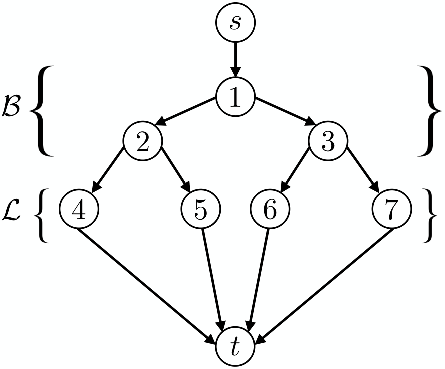
A formal definition for the flow graph associated with a balanced decision tree is as follows.
Definition 2.2 (Flow Graph of a Balanced Decision Tree)
Given a balanced decision tree of depth , define the directed flow graph associated with the tree as follows. Let be the vertices of the flow graph. Given , let be the left descendant of , be the right descendant of , and
be the arcs of the graph. Also, given , let be the ancestor of , defined through and if .
2.2 Problem Formulation
Let be a training dataset consisting of datapoints indexed in the set . Each row consists of binary features indexed in the set , which we collect in the vector , and a label drawn from the finite set of classes. In this section we formulate the problem of learning a multi-class classification tree of fixed finite depth that minimizes the misclassification rate (or equivalently, maximizes the number of correctly classified datapoints) based on MIO technology.
In our formulation, the classification tree is described through the branching variables and the prediction variables . In particular, we use the variables , , , to indicate if the tree branches on feature at branching node (i.e., it equals 1 if and only if the binary test performed at asks ‘‘is ’’?). Accordingly, we employ the variables , , , to indicate that at leaf node the tree predicts class . We use the auxiliary routing/flow variables to decide on the flow of data through the flow graph associated with the decision tree. Specifically, for each node and for each datapoint , we introduce a decision variable which equals 1 if and only if the th datapoint is correctly classified and its flow traverses the arc on its way to the sink . We let be defined accordingly for each arc between node and sink . Datapoint is correctly classified if and only if its corresponding flow passes through some leaf node such that , i.e., where the class predicted coincides with the class of the datapoint. If the flow of a datapoint arrives at such a leaf node and the datapoint is correctly classified, its corresponding flow is directed to the sink, i.e., ; otherwise, the corresponding flow is not initiated from the source at all. With these variables, the flow-based formulation reads
| maximize | (1a) | ||||
| subject to | (1b) | ||||
| (1c) | |||||
| (1d) | |||||
| (1e) | |||||
| (1f) | |||||
| (1g) | |||||
| (1h) | |||||
| (1i) | |||||
| (1j) | |||||
| (1k) | |||||
| (1l) | |||||
| (1m) | |||||
An interpretation of the constraints and objective is as follows. Constraints (1b) ensure that at each branching node we branch on exactly one feature . Constraints (1c) are flow conservation constraints for each datapoint and node : they ensure that if a datapoint arrives at a node, then it must also leave the node through one of its descendants. Similarly, constraints (1d) enforce flow conservation for each node . The inequality constraints (1e) imply that at most one unit of flow can enter the graph through the source for each datapoint. Constraints (1f) (resp. (1g)) ensure that if the flow of a datapoint is routed to the left (resp. right) at node , then one of the features such that (resp. ) must have been selected for branching at the node. Constraints (1h) guarantee that datapoints whose flow is routed to the sink node are correctly classified. Constraints (1i) make sure that each leaf node is assigned a predicted class . The objective (1a) maximizes the total number of correctly classified datapoints.
Formulation (1) has several distinguishing features relative to existing MIO formulations for training decision trees: First, it does not use big- constraints. Second, it includes flow variables indicating whether each datapoint is directed to the left or right at each branching node, which resembles the well-known multi-commodity flow concept, see Hu 1963. Third, incorrectly classified datapoints are associated with a flow of zero. In contrast, previous formulations (Bertsimas and Dunn 2017, Verwer and Zhang 2019) and more sophisticated formulations we propose later in Section 4 include binary decision variables that indicate the leaf each datapoint lands on. The advantage of modeling misclassified points with a flow of zero is that the resulting formulation is smaller. A similar idea of ‘‘projecting out’’ variables associated with misclassified datapoints was proposed by Günlük et al. 2021.
The number of variables and constraints in Problem (1) is , where is the tree depth. Thus, its size is of the same order as the univariate splits formulation of Bertsimas and Dunn 2017 (formulation (24) in their paper) while being of higher order than that of Verwer and Zhang 2019. Nonetheless, the LO relaxation of formulation (1) is tighter than those of Bertsimas and Dunn 2017 and Verwer and Zhang 2019, as demonstrated in the following theorem which we prove in Electronic Companion 10, and therefore results in a more aggressive pruning of the branch-and-bound tree.
Theorem 2.3
Problem (1) has a stronger LO relaxation than the formulations of Bertsimas and Dunn 2017 and Verwer and Zhang 2019.
Remark 2.4
Formulation (1) assumes that all features are binary. However, this formulation can also be applied to datasets involving categorical or bounded integer features by first preprocessing the data as follows. For each categorical feature, we encode it as a one-hot vector, i.e., for each level of the feature, we create a new binary column which has value 1 if and only if the original column has the corresponding level. We follow a similar approach for encoding integer features with a slight change. The new binary column has value 1 if and only if the main column has the corresponding value or any value smaller than it, see e.g., Verwer and Zhang 2019 and Okada et al. 2019. This discretization of the features increases the size of the dataset linearly with the number of possible values of each categorical/integer feature. We also note that formulation (1) only considers univariate splits. It can however be generalized to allow for multivariate splits. Indeed, in the case of binary features, having multivariate (or oblique) splits is equivalent to ‘‘combinatorial’’ branching, which can be done by creating additional artificial features, see Günlük et al. 2021 for additional discussion. We can also extend formulation (1) for the case of non-binary trees, where each splitting node can have more than two children. This can be achieved by introducing additional nodes and edges to the flow graph while adjusting the formulation accordingly.
3 Benders’ Decomposition via Facet-defining Cuts
In Section 2, we proposed a formulation for designing optimal classification trees that is provably stronger than existing approaches from the literature. Our model presents an attractive decomposable structure that we leverage in this section to speed-up computation.
3.1 Main Problem, Max-Flow Subproblems, and Benders’ Decomposition
A classification tree is uniquely characterized by the branching decisions and predictions made at the branching nodes and leaves, respectively. Given a choice of and , each datapoint in problem (1) is allotted one unit of flow that can be guided from the source node to the sink node through the flow graph associated with the decision tree. If the datapoint cannot be correctly classified, the flow that will reach the sink (and by extension enter the source) will be zero. In particular, once the branching variables and prediction variables have been fixed, optimization of the auxiliary flow variables can be done separately for each datapoint. In particular, we can decompose problem (1) into a main problem involving the variables , and subproblems indexed by each involving the flow variables associated with datapoint . Additionally, each subproblem is a maximum flow problem for which specialized polynomial-time methods exist. Due to these characteristics, formulation (1) can be naturally tackled using Benders’ decomposition, see Benders 1962. In what follows, we describe the Benders’ decomposition approach.
Problem (1) can be written equivalently as:
| maximize | (2a) | ||||
| subject to | (2b) | ||||
| (2c) | |||||
| (2d) | |||||
| (2e) | |||||
where, for any fixed , and , the quantity is defined as the optimal objective value of the problem
| (3a) | |||||
| subject to | (3b) | ||||
| (3c) | |||||
| (3d) | |||||
| (3e) | |||||
| (3f) | |||||
| (3g) | |||||
| (3h) | |||||
| (3i) | |||||
Problem (3) is a maximum flow problem on the flow graph , see Definition 2.2, whose arc capacities are determined by and datapoint , as formalized next.
Definition 3.1 (Capacitated flow graph)
Given the flow graph , vectors , and datapoint , define arc capacities as follows. Let , and for all , and for . Define the capacitated flow graph as the flow graph augmented with capacities .
Observe that the arc capacities in are affine functions of . An interpretation of the arc capacities and capacitated flow graph for and feasible in problem (2) is as follows. Constraints (2b) imply that the weights , , in the above definition are binary. Indeed, the capacity of the arc incoming into node 1 is 1. Moreover, for each node and datapoint , exactly one of the outgoing arcs of node in graph has capacity 1: the left arc if the datapoint passes the test () or the right arc if it fails it (). Finally, for each node in graph , its outgoing arc has capacity one if and only if the datapoint has the same label as that predicted at node . Thus, for each datapoint, the set of arcs with capacity 1 in the graph forms a path from the source node to the leaf where this datapoint is assigned in the decision tree. This path is connected to the sink via an arc of capacity 1 if and only if the datapoint is correctly classified. We note that as all the arc capacities in the flow graph are binary, the integrality constraints (3h) and (3i) can be relaxed.
Problem (3) is equivalent to a maximum flow problem on the capacitated flow graph . From the well-known max-flow/min-cut duality, see e.g., Vazirani 2013, it follows that is the capacity of a minimum cut of graph . In other words, it is the greatest value smaller than or equal to the value of all cuts in graph . Given a set , we let denote the cut-set corresponding to the source set . With this notation, problem (2) can be reformulated as
| (4a) | |||||
| subject to | (4b) | ||||
| (4c) | |||||
| (4d) | |||||
| (4e) | |||||
| (4f) | |||||
| (4g) | |||||
where, at an optimal solution, represents the value of a minimum cut of graph . Indeed, the objective function (4a) maximizes the , while constraints (4b) ensure that the value of is no greater than the value of a minimum cut.
Formulation (4) contains an exponential number of inequalities (4b) and is implemented using row generation, whereby constraints (4b) are initially dropped and added on the fly during optimization as Benders’ cuts. Note that we added the redundant constraints (4g) to ensure problem (4) is bounded even if all constraints (4b) are dropped. Row generation can be implemented in modern MIO solvers via callbacks, by adding lazy constraints at relevant nodes of the branch-and-bound tree. Identifying which constraint (4b) to add can in general be done by solving a minimum cut problem, and could in principle be solved via well-known algorithms, such as Goldberg and Tarjan 1988 and Hochbaum 2008.
The Benders’ method we propose is reminiscent of the approach proposed by Lozano and Smith 2022 to tackle two-stage problems in which the subproblem corresponds to a ‘‘tractable’’ 0-1 problem (i.e., a problem that admits an exact LO reformulation). In Lozano and Smith 2022, this subproblem is a decision diagram; in our case, it is a maximum flow problem. Thus, inequalities (4b) correspond to usual Benders’ cuts, that replace the discrete subproblem with its (equivalent) continuous LO reformulation. As also pointed out by Lozano and Smith 2022, at each iteration of Benders’ method, there are often multiple optimal dual solutions, each corresponding to a candidate inequality that can be added. Cuts obtained from most of these solutions might be weak in general, and thus they discuss how to strengthen them. In the next section, we propose a method that, among all potential optimal dual solutions, finds one that is guaranteed to result in a facet-defining cut for the convex hull of the feasible region given by inequalities (4b)-(4g), that is, a cut that is already the best possible and admits no further strengthening. In addition, the method is faster than using a general purpose method to find minimum cuts or solve LO problems which we show in Electronic Companion 13.1.
3.2 Generating Facet-Defining Cuts via a Tailored Min-Cut Procedure
Row generation methods for integer optimization problems such as Benders’ decomposition may require a long time to converge to an optimal solution if each added inequality is weak for the feasible region of interest. It is therefore of critical importance to add strong non-dominated cuts at each iteration of the algorithm, e.g., see Magnanti and Wong 1981. We now argue that not all inequalities (4b) are facet-defining for the convex hull of the feasible set of problem (4). To this end, let represent the (mixed-binary) feasible region defined by constraints (4b)-(4g), and denote by its convex hull. Example 3.2 below shows that some of inequalities (4b) are not facet-defining for –even if they correspond to a minimum cut for a given value of – and are in fact dominated.
Example 3.2
Consider an instance of problem (4) with a depth decision tree (i.e., and ) and a dataset involving a single feature (). Consider datapoint such that and . Suppose that the solution to the main problem is such that we branch on (the unique) feature at node 1 and predict class at nodes 2 and 3. Then, datapoint is routed left at node 1 and is misclassified. A valid min-cut for the resulting graph includes all arcs incoming into the sink, i.e., and . The associated Benders’ inequality (4b) reads
| (5) |
Intuitively, (5) states that datapoint can be correctly classified if its class label is assigned to at least one node, and is certainly valid for . However, since datapoint cannot be routed to node , the stronger inequality
| (6) |
is valid for and dominates (5).
Example 3.2 implies that an implementation of formulation (4) using general purpose min-cut algorithms to identify constraints to add may perform poorly. This motivates us to develop a tailored algorithm that exploits the structure of each capacitated flow graph to return inequalities that are never dominated, thus resulting in faster convergence of the Benders’ decomposition approach.
Algorithm 1 shows the proposed procedure, which can be called at integer nodes of the branch-and-bound tree, using for example callback procedures available in most commercial and open-source solvers. Algorithm 1 traverses the flow graph associated with a datapoint using depth-first search to investigate the existence of a path from the source to the sink. If there is such a path, it means that the datapoint is correctly classified and there are no violating inequalities. Otherwise, it outputs the set of all observed nodes in the traverse as the source set of the min-cut. Figure 2 illustrates Algorithm 1. We now prove that Algorithm 1 is indeed a valid separation algorithm.
Input:
Output: if all constraints (4b) corresponding to are satisfied;
source set of min-cut otherwise.
Proposition 3.3
Proof 3.4
Proof. Note that the right-hand side of (4b), which corresponds to the capacity of a cut in the graph, is nonnegative. Therefore, if (line 1), all inequalities are automatically satisfied. Since is integer, all arc capacities are either 0 or 1. We assume that the arcs with zero capacity are removed from the flow graph. Moreover, since , we find that either the value of a minimum cut is and there exists a violated inequality, or the value of a minimum cut is at least and there is no violated inequality. Finally, there exists a 0-capacity cut if and only if and belong to different connected components in the graph .
The connected component belongs to, can be found using depth-first search. For any fixed , constraints (4c) and the definition of imply that either arc or arc has capacity 1 (but not both). If arc has capacity 1 (line 6), then can be added to the component connected to (set ); the case where arc has capacity 1 (line 8) is handled analogously. This process continues until a leaf node is reached (line 12). If the capacity of the arc to the sink is 1 (line 15), then an path is found and no cut with capacity exists. Otherwise (line 13), is the connected component of and , thus is the source of a minimum cut with capacity .\halmos
Observe that Algorithm 1, which exploits the specific structure of the network for binary feasible in (2), is much faster than general purpose minimum-cut methods. Indeed, since at each iteration in the main loop (lines 4-11), the value of is updated to a descendant of , the algorithm terminates in at most iterations, where is the depth of the tree. As is , the complexity is logarithmic in the size of the tree. In addition to providing a very fast method for generating Benders’ inequalities at integer nodes of a branch-and-bound tree, Algorithm 1 is guaranteed to generate strong non-dominated inequalities.
Define
Our main motivation for introducing is that is full dimensional, whereas is not. Moreover, in formulation (4), apart from constraints (4c)-(4d), variables and only appear in the right-hand side of inequalities (4b) with non-negative coefficients. Therefore, replacing constraints (4c)-(4f) with still results in valid formulation for problem (4), since there exists an optimal solution where the inequalities are tight. Theorem 3.5 below formally states that Algorithm 1 generates non-dominated inequalities.
Theorem 3.5
All violated inequalities generated by Algorithm 1 are facet-defining for .
Example 3.6 (Example 3.2 Continued)
Remark 3.7
Algorithm 1 can only be invoked at integer nodes of the branch-and-bound tree. However, there is a slight advantage in including as many cut-set inequalities as possible at the root node of the branch-and-bound tree by utilizing Gurobi to solve the corresponding linear optimization problem for each subproblem. This approach allows us to enhance the LO relaxation at integer nodes. A detailed investigation on this matter is reported in Electronic Companion 13.1.
4 Generalizations
In Section 2, we proposed a flow-based MIO formulation for designing optimal balanced decision trees, see problem (1). In this section, we generalize this core formulation to design regularized (i.e., not necessarily balanced) classification trees wherein the distance from root to leaf may vary across leaves. We also discuss a variant that tracks all datapoints, even those that are not correctly classified, making it suitable to learn from imbalanced datasets, and to design fair decision trees.
4.1 Imbalanced Decision Trees
Formulation (1) outputs a balanced decision tree as defined in Definition 2.1. Such trees may result in over-fitting of the data and poor out-of-sample performance, in particular if is large. To this end, we propose a variant of formulation (1) which allows for the design of trees that are not necessarily balanced and that have the potential of performing better out-of-sample. To this end, we introduce the following terminology pertaining to imbalanced trees.
Definition 4.1 (Imbalanced Decision Trees)
An imbalanced decision tree of (maximum) depth is a full binary tree, i.e., a tree in which every node has either 0 or 2 children and where the largest depth of a leaf is . We let denote the set of all candidate branching nodes and represent the set of terminal nodes. We will refer to a node as a leaf if no branching occurs at the node.
Note that in a balanced decision tree, see Definition 2.1, branching occurs at all nodes in , and leaves of the decision tree correspond precisely to all nodes of maximum depth, i.e., . In contrast, in imbalanced decision trees nodes in can be leaf nodes and terminal nodes in need not be part of the decision tree.
Akin to Definition 2.2, we associate with an imbalanced decision tree a directed acyclic graph by augmenting the tree with a single source node that is connected to the root node of the tree and a single sink node that is connected to all nodes of the tree, allowing correctly classified datapoints to flow to the sink from any node where a prediction is made (leaf of the learned tree). An illustration of these concepts on an imbalanced decision tree of depth is provided on Figure 3. A formal definition for the flow graph associated with a imbalanced decision tree of maximum depth is as follows.


Definition 4.2 (Flow Graph of an Imbalanced Decision Tree)
Given an imbalanced decision tree of depth , we define its associated directed flow graph as follows. Let be the vertices of the flow graph. Given , let be the left descendant of , be the right descendant of , and
be the arcs of the graph. Also, given , let be the parent of , defined through and if .
We are now ready to formulate the variant of problem (1) that allows for the design of imbalanced classification trees. In addition to the decision variables from formulation (1) we introduce, for every node , the binary decision variable which has a value of one if and only if node is a leaf node of the tree, i.e., if we make a prediction at node . The auxiliary routing/flow variables now account for all arcs in the flow graph introduced in Definition 4.2. The problem of learning optimal imbalanced classification trees is then expressible as
| maximize | (7a) | ||||
| subject to | (7b) | ||||
| (7c) | |||||
| (7d) | |||||
| (7e) | |||||
| (7f) | |||||
| (7g) | |||||
| (7h) | |||||
| (7i) | |||||
| (7j) | |||||
| (7k) | |||||
| (7l) | |||||
| (7m) | |||||
| (7n) | |||||
where is the set of all ancestors of node , i.e., the set of all nodes lying on the unique path from the root node to node , and is a regularization parameter. An explanation of the new/modified problem constraints is as follows. Constraints (7b) imply that at any node we either branch on a feature (if ), predict a label (if ), or get pruned if a prediction is made at one of the node ancestors (i.e., if ). Similarly constraints (7c) ensure that any node is either a leaf node of the tree or is pruned. Constraints (7d)-(7j) exactly mirror constraints (1c)-(1i) in problem (1). They are slight modifications of the original constraints accounting for the new arcs added to the flow graph and for the possibility of making predictions at branching nodes . In particular, constraints (7j) imply that if a node gets pruned we do not predict any class at the node, i.e., for all . A penalty term is added to (7a), to encourage sparser trees with fewer branching decisions. Note that while it is feasible to design a decision tree with the same branching decisions in multiple nodes on a single path from root to sink, such solutions are never optimal for (7) if , as a simpler tree would result in the same misclassification.
Problem (7) allows for the design of regularized decision trees by augmenting this nominal formulation with additional regularization constraints. These either limit or penalize the number of nodes that can be used for branching or place a lower bound on the number of datapoints that land on each leaf. We detail these variants in the following. All of these variants either explicitly or implicitly restrict the tree size, thereby mitigating the risk of overfitting and resulting in more interpretable trees.
Sparsity.
A commonly used approach to restrict tree size is to add sparsity constraints which restrict the number of branching nodes, see e.g., Breiman et al. 1984, Quinlan 2014, Bertsimas and Dunn 2017, Aghaei et al. 2019, and Blanquero et al. 2020. Such constraints are usually met in traditional methods by performing a post-processing pruning step on the learned (unrestricted) tree. We enforce this restriction by adding the constraint
| (8) |
to problem (7), and possibly setting . This constraint ensures that the learned tree has at most branching nodes (thus at most leaf nodes), where is a hyper-parameter that can be tuned using cross-validation, see e.g., Bishop 2006. We note that due to the non-convexity introduced by the integer variables in problem (7), the constrained sparsity formulation provides more options than the penalized version, see e.g., Lombardi et al. 2020. In other words, for any choice of in the penalized version, there exists a choice of in the constrained version that yields the same solution, but the converse is not necessarily true. The penalized version is more common in the machine learning literature and we will thus use it for benchmarking purposes in our numerical results, see Section 5.
Maximum Number of Features to Use.
One can also constrain the total number of features branched on in the decision tree as in Aghaei et al. 2019 by adding the constraints
| (9) |
to problem (7), where , , are decision variables that indicate if feature is used in the tree. Parameter can be a user-specified input or tuned via cross-validation. Note that neither integrality nor bound constraints on variable need to be enforced in the formulation.
Minimum Number of Datapoints in each Leaf Node.
Another popular regularization approach, see e.g., Bertsimas and Dunn 2017, consists in placing a lower bound on the number of datapoints that land in each leaf. To ensure that each node contains at least datapoints, we impose
| (10) |
in problem (7).
4.2 Imbalanced Datasets
A dataset is called imbalanced when the class distribution is not uniform, i.e., when the number of datapoints in each class varies significantly from class to class. In the case when a dataset consists of two classes, i.e., , we say that it is imbalanced if
in which case and are referred to as the majority and minority classes, respectively. In imbalanced datasets, predicting the majority class for all datapoints results in high accuracy, and thus decision trees that maximize prediction accuracy without accounting for the imbalanced nature of the data perform poorly on the minority class. Imbalanced datasets occur in many important domains, e.g., to predict landslides, to detect fraud, or to predict if a patient has cancer, e.g., see, Kirschbaum et al. 2009, Wei et al. 2013, and Khalilia et al. 2011. Naturally, being able to predict the minority class(es) accurately is crucial in such settings.
In the following we propose adjustments to the core formulation (7) to ensure meaningful decision trees are learned even in the case of imbalanced datasets. These adjustments require calculating metrics such as true positives, true negatives, false positives, and false negatives or some function of them such as recall (fraction of all datapoints from the positive class that are correctly identified) and precision (the portion of correctly classified datapoints from the positive class out of all datapoints with positive predicted class). Thus, learning meaningful decision trees requires us to track all datapoints, not only the correctly classified ones as done in formulations (1) and (7).
To this end, we propose to replace the single sink in the flow graph associated with a imbalanced decision tree, see Definition 4.2, with sink nodes denoted by , one for each class . Each sink node , , is connected to all nodes and collects all datapoints (both correctly and incorrectly classified) with predicted class .
A formal definition for the flow graph associated with a decision tree that can be used to train imbalanced decision trees and that can track all datapoints is as follows.
Definition 4.3 (Complete Flow Graph of an Imbalanced Decision Tree)
Given a decision tree of depth , we define the directed complete flow graph associated with the tree that can be used to learn imbalanced decision trees of maximum depth and that tracks all datapoints through the graph as follows. Let be the vertices of the flow graph. Given , let , , and be as in Definition 4.2 and let
be the arcs of the graph.
We are now ready to formulate the variant of problem (7) that tracks all datapoints through the flow graph with sink nodes , . In a way that parallels formulation (7), we introduce auxiliary variables for each node and each class to track the flow of datapoints (both correctly classified and missclassified) to the sink node . Our formulation reads
| maximize | (11a) | ||||
| subject to | (11b) | ||||
| (11c) | |||||
| (11d) | |||||
| (11e) | |||||
| (11f) | |||||
| (11g) | |||||
| (11h) | |||||
| (11i) | |||||
| (11j) | |||||
| (11k) | |||||
| (11l) | |||||
| (11m) | |||||
| (11n) | |||||
An interpretation of the problem constraints is as follows. Constraints (11b)-(11j) exactly mirror constraints (7b)-(7j) in problem (7). There are three main differences in these constraints. Flow conservation constraints (11d) and (11e) now allow flow to be directed to any one of the sink nodes from any one of the nodes . Constraints (11f) ensure that the flow incoming into the source and associated with each datapoint equals 1. Constraints (11i) stipulate that a datapoint is only allowed to be directed to the sink corresponding to the class predicted at the leaf where the datapoint landed. Constraints (11d)-(11f) and (11i) together ensure that all datapoints get routed to the sink associated with their predicted class. As a result of these changes, sink node collects all datapoints, whether correctly classified or not, with predicted class . The objective (11a) is updated to reflect that a datapoint is correctly classified if and only if it flows to sink .
At a feasible solution to problem (11), the quantity represents the total number of datapoints that land at node . The number of datapoints of class that are correctly (resp. incorrectly) classified is expressible as (resp. ), while the total number of datapoints for which we predict class can be written as .
Problem (11) allows us to learn meaningful decision trees for the case of imbalanced data by modifying the objective function of the problem and/or by augmenting this nominal formulation with constraints. We detail these variants in what follows.
Balanced Accuracy.
A common approach to handle imbalanced datasets is to optimize the so-called balanced accuracy, which averages the accuracy across classes. Intuitively, in the case of two classes, it corresponds to the average of the true positive and true negative rates, see e.g., Mower 2005. It can also be viewed as the average between sensitivity and specificity. Maximizing balanced accuracy can be achieved by replacing the objective function of problem (11) with
Each term in the summation above represents the proportion of datapoints from class that are correctly classified. Having high balanced accuracy is important when dealing with imbalanced data and correctly predicting all classes is (equally) important.
Worst-Case Accuracy.
As a variant to optimizing the average accuracy across classes, we propose to maximize the worst-case (minimum) accuracy. This can be achieved by replacing the objective function of problem (11) with
To the best of our knowledge, this idea has not been proposed in the literature. Compared to minimizing average accuracy, this objective attaches more importance to the class that is ‘‘worse-off.’’ Having high worst-case accuracy is important when dealing with imbalanced data and correctly predicting the class that is the hardest to predict is important. This is the case for example when diagnosing cancer where positive cases are hard to identify and having large false negative rates (i.e., low true positive rate) could cost a patient’s life. There are also related works on robust classification where the objective happens to be the minimization of worst-case accuracy over noisy features/labels, see Bertsimas et al. 2019a, or over adversarial examples, see Vos and Verwer 2021.
In the remaining of this section we focus on the case of binary classification where and we refer to (resp. ) as the positive (resp. negative) class. In this setting we can discuss metrics such as recall, precision, sensitivity, and specificity more conveniently. Naturally, these definitions can be generalized to cases with more classes.
Constraining Recall.
An important metric in the classification problem when dealing with imbalanced datasets is recall (also referred to as sensitivity), which is the fraction of all datapoints from the positive class that are correctly identified. Guaranteeing a certain level of recall can be achieved by augmenting problem (11) with the constraint
Decreasing the number of false negatives (datapoints from the positive class that are incorrectly predicted) increases recall. Thus, in cases where false negatives can have dramatic consequences and even cost lives, such as in cancer diagnosis or when predicting landslides, guaranteeing a certain level of recall can help mitigate such risks.
Constraining Precision.
Our method can conveniently be used to learn decision trees that have sufficiently high precision, which is defined as the portion of correctly classified datapoints from the positive class out of all datapoints with positive predicted class. This can be achieved by augmenting problem (11) with the constraint
| (12) |
where is a hyper-parameter that represents the minimum acceptable precision that can be tuned via cross-validation. Decreasing the number of false positives (datapoints from the negative class that are incorrectly classified) increases precision. Thus, constraining precision is useful in settings where having a low number of false negatives is not as important and having a low number of false positives, such as when making product recommendations.
Balancing Sensitivity and Specificity.
Günlük et al. 2021 address the issue of imbalanced data by maximizing sensitivity (true positive rate) in the objective, while guaranteeing a certain level of specificity (true negative rate), or the converse, instead of optimizing the total accuracy. In the case of binary classification where , we can constrain specificity from below by augmenting problem (11) with the constraint
and maximize sensitivity by replacing its objective function with
This method is useful in settings such as infectious disease testing wherein we want to maximize the chance of correctly predicting someone to be infectious while making sure to identify non-infectious individuals with a high enough confidence.
4.3 Learning Fair Decision Trees
In recent years, machine learning algorithms are increasingly being used to assist decision-making in socially sensitive, high-stakes, domains. For example, they are used to help decide who to give access to credit, benefits, and public services, see e.g., Byrnes 2016 and Azizi et al. 2018, to help guide policing, see e.g., Rudin 2013, or to assist with screening decisions for jobs/college admissions, see e.g., Miller 2015. Yet, decision-making systems based on standard machine learning algorithms may result in discriminative decisions as they may treat or impact individuals unequally based on certain characteristics, often referred to as protected or sensitive, including but not limited to age, disability, ethnicity, gender, marital status, national origin, race, religion, and sexual orientation, see e.g., Dwork et al. 2012, Angwin et al. 2016, and Barocas and Selbst 2016.
Over the last decade, so-called ‘‘in-process’’ fair machine learning algorithms have been proposed as a way to mitigate bias in standard ML. These methods incorporate a fairness notion, such as statistical parity (Dwork et al. 2012) or equalized odds (Hardt et al. 2016) in the training step, either penalizing or constraining discrimination. Notably, several in-process approaches have been proposed for learning fair decision trees. The vast majority of these methods are based on heuristics. For example, Kamiran et al. 2010 and Zhang and Ntoutsi 2019 propose to augment the splitting criterion of CART and of the Hoeffding Tree algorithm, respectively, with a regularizer to promote statistical parity and accuracy. Grari et al. 2019 propose a fair gradient boosting algorithm to design fair decision trees that satisfy either equalized odds or statistical parity. Ranzato et al. 2021 introduce a genetic algorithm for training decision trees that maximize both accuracy and robustness to adversarial perturbations and accounting for individual fairness. In contrast with the aforementioned works, Aghaei et al. 2019 propose an MIO based formulation involving a fairness regularizer in the objective aimed at mitigating disparate treatment and disparate impact, see Barocas and Selbst 2016. While this approach has proved effective relative to heuristics, it is based on a weak formulation and is therefore slow to converge, see Section 1.
In this section, we discuss how our stronger formulation (11) can be augmented with fairness constraints to learn optimal and fair decision trees satisfying some of the most common fairness requirements in the literature. We refer the interested reader to the book by Barocas et al. 2019 and to the survey papers of Corbett-Davies and Goel 2018, Mehrabi et al. 2021 and Caton and Haas 2020 and to the references there-in for in-depth reviews of the literature on the topic of fair ML including analyses on the relative merits of various fairness metrics.
Throughout this section, and for ease of exposition, we consider the case of binary classification where . We let correspond to the positive outcome. For example, in a hiring problem where we want to decide whether to interview someone or not, being invited for an interview is regarded as the positive outcome. We let denote the value of the protected feature (s) of datapoint , where denotes the set of all possible levels of the protected feature (s). Depending on whether branching on the protected feature is allowed or not, can either be included or excluded as an element of the feature vector , see e.g., Gajane and Pechenizkiy 2017 and Chen et al. 2019a.
Statistical Parity.
A classifier satisfies statistical parity if the probability of predicting the positive outcome is similar across all the protected groups, see Dwork et al. 2012. For example in the hiring problem mentioned above, it may be appropriate to impose that the probability of receiving an interview should be similar across genders if people from different genders are equally likely to be meritorious. Augmenting model (11) with the following constraints ensures that the decision tree learned by our MIO formulation satisfies statistical parity up to a bias
where the first and second term correspond to empirical estimates of the conditional probabilities of predicting the positive outcome given and , respectively.
Conditional Statistical Parity.
A classifier satisfies conditional statistical parity across protected groups if the probability of predicting the positive outcome is similar between all groups conditional on some feature, e.g., a legitimate feature that can justify differences across protected groups, see Corbett-Davies et al. 2017. We let denote the value of the feature (s) of datapoint that can legitimize differences, where denotes the set of all possible levels of the legitimate feature(s). For example, in the problem of matching people experiencing homelessness to scarce housing resources, it is natural to require that the probability of receiving a resource among all individuals with the same vulnerability (a risk score) should be similar across genders, races, or other protected attribute. By adding the following constraints to model (11), we can ensure our learned trees satisfy conditional statistical parity up to a bias given any value
where the first and second term correspond to empirical estimates of the conditional probabilities of predicting positive outcome given and , respectively, conditional on .
Predictive Equality.
A classifier satisfies predictive equality if it results in the same false positive rates across protected groups, see Chouldechova 2017. For example, this fairness notion may be useful when using machine learning to predict if a convicted person will recidivate so as to decide if it is appropriate to release them on bail, see Angwin et al. 2016. Indeed, predictive equality in this context requires that, among defendants who would not have gone on to recidivate if released, detention rates should be similar across all races. Adding the following constraints to model (11) ensures that the learned decision trees satisfy predictive equality, up to a constant
where the first and second terms inside the absolute value are the estimated false positive rate given and , respectively.
Equalized Odds.
A classifier satisfies equalized odds if the predicted outcome and protected feature are independent conditional on the outcome, see Hardt et al. 2016. In other words, equalized odds requires same true positive rates and same false positive rates across protected groups. For example, in the college admissions process, equalized odds requires that no matter the applicant’s gender, if they are qualified (or unqualified), they should get admitted at equal rates. By adding the following constraints to model (11) we ensure the decision trees learned by our MIO formulation satisfy equalized odds up to a constant
where the first and second terms correspond to empirical estimates of conditional probabilities of predicting the positive outcome given and , respectively. If we relax the above constraints to only hold for , we achieve equal opportunity up to a constant , see Hardt et al. 2016.
All the introduced nonlinear constraints can be linearized using standard MIO techniques. We leave this task to the reader. Our approach can also impose fairness by means of regularization and can also model more sophisticated fairness metrics such as the ones of Aghaei et al. 2019. We leave these extensions to the reader.
4.4 Solution Approach for Generalizations
We now briefly discuss how to solve formulation (7) (for learning imbalanced decision trees), and formulation (11) (which tracks all datapoints through the flow graph), and their variants introduced in Sections 4.1 through 4.3.
The nominal formulations (7) and (11) and all their variants augmented with constraints that do not couple datapoints with one another (e.g., sparsity constraints (8) or interpretability constraints (9)) can be effectively solved using Benders’ decomposition. This can be achieved by adapting Algorithm 1 from Section 3. On the other hand, when these formulations are augmented with constraints that do couple datapoints with one another (like the fairness constraints from Section 4.3), Benders’ decomposition is no longer applicable. In such cases, these formulations need to be solved directly as monolithic MIO problems.
5 Experiments
In the following section, we discuss the datasets we use in our experiments, the approaches that we compare to, the experimental setup, and our findings. More extensive numerical results are included in the electronic companion.
5.1 Benchmark Approaches and Datasets
In our numerical experiments, we have two sets of experiments, one on datasets with only categorical features and one on datasets with a mixture of categorical and real-valued features. We now describe both sets of data and the approaches we compare to in each case.
Datasets with only Categorical Features.
In the first part of our experiments we use all twelve publicly available datasets with only categorical features from the UCI data repository (Dua and Graff 2017) as detailed in Table 1. We compare the flow-based formulation (FlowOCT) given in problem (7) and its Benders’ decomposition (BendersOCT) described in Electronic Companion 11 to the univariate splits formulations proposed by Bertsimas and Dunn 2017 (OCT) and Verwer and Zhang 2019 (BinOCT). We also compare to the heuristic algorithm based on local search for solving OCT proposed by Bertsimas and Dunn 2019 (LST). As the code used for OCT is not publicly available, we implemented the corresponding formulation (adapted to the case of binary data). The details of this implementation are given in Electronic Companion 8. We also used the Python implementation of LST which is available for academic use. In LST, we set the complexity parameter ‘cp’ to 0 which is analogous to setting . In order to make the optimality gap comparable across approaches, we made some adjustments to the objective function of FlowOCT and BendersOCT, by subtracting number of total datapoints from the objective, such that, for all approaches, the objective value reflects the number of misclassified datapoints. The results for worst-case accuracy objective discussed in Section 4.2 can be found in Electronic Companion 13.2. We also numerically analyze the strength of all formulations by looking at their LO relaxation, see Electronic Companion 13.3. Analysis of some implementation variants of BendersOCT, see Remark 3.7, can be found in Electronic Companion 13.1
| Dataset | |||
|---|---|---|---|
| soybean-small | 47 | 45 | 4 |
| monk3 | 122 | 15 | 2 |
| monk1 | 124 | 15 | 2 |
| hayes-roth | 132 | 15 | 3 |
| monk2 | 169 | 15 | 2 |
| house-votes-84 | 232 | 16 | 2 |
| spect | 267 | 22 | 2 |
| breast-cancer | 277 | 38 | 2 |
| balance-scale | 625 | 20 | 3 |
| tic-tac-toe | 958 | 27 | 2 |
| car-evaluation | 1728 | 20 | 4 |
| kr-vs-kp | 3196 | 38 | 2 |
Datasets with Mixed Features.
In the second part of our experiments, we use 28 publicly available datasets with both categorical and real-valued features from the UCI data repository as detailed in Table 2. In this part, we compare BendersOCT to OCT. We did not include BinOCT as it cannot handle real-valued features. We also did not include FlowOCT as it is outperformed by BendersOCT. To run BendersOCT on these datasets, we first discretize the real-valued features into and buckets (quantiles) and then one-hot encode the discretized columns. We refer to the version of BendersOCT which we run on the discretized data with 5 (resp. 10) buckets as BendersOCT-5 (resp. BendersOCT-10). As OCT can handle real-valued features without special encoding, we use the original format of the datasets for OCT. For both OCT and BendersOCT the categorical features are one-hot encoded.
| Dataset |
|
|
|
||||||||
|---|---|---|---|---|---|---|---|---|---|---|---|
| echocardiogram | 61 | 8 | 32 | 61 | 2 | ||||||
| hepatitis | 80 | 19 | 43 | 68 | 2 | ||||||
| fertility | 100 | 20 | 28 | 28 | 2 | ||||||
| iris | 150 | 4 | 20 | 38 | 3 | ||||||
| wine | 178 | 13 | 65 | 130 | 3 | ||||||
| planning-relax | 182 | 12 | 60 | 120 | 2 | ||||||
| breast-cancer-prognostic | 194 | 33 | 164 | 321 | 2 | ||||||
| parkinsons | 195 | 22 | 110 | 218 | 2 | ||||||
| connectionist-bench-sonar | 208 | 60 | 300 | 600 | 2 | ||||||
| seeds | 210 | 7 | 35 | 70 | 3 | ||||||
| cylinder-bands | 277 | 257 | 314 | 370 | 2 | ||||||
| heart-cleveland | 297 | 22 | 44 | 68 | 5 | ||||||
| ionosphere | 351 | 33 | 157 | 298 | 2 | ||||||
| thoracic-surgery | 470 | 27 | 39 | 54 | 2 | ||||||
| climate | 540 | 18 | 90 | 180 | 2 | ||||||
| breast-cancer-diagnostic | 569 | 30 | 150 | 300 | 2 | ||||||
| indian-liver-patient | 579 | 10 | 45 | 88 | 2 | ||||||
| credit-approval | 653 | 42 | 64 | 89 | 2 | ||||||
| blood-transfusion | 748 | 4 | 20 | 36 | 2 | ||||||
| diabetes | 768 | 8 | 39 | 75 | 2 | ||||||
| qsar-biodegradation | 1055 | 41 | 139 | 234 | 2 | ||||||
| banknote-authentication | 1372 | 4 | 20 | 40 | 2 | ||||||
| ozone-level-detection-one | 1848 | 72 | 358 | 714 | 2 | ||||||
| image-segmentation | 2310 | 18 | 82 | 164 | 7 | ||||||
| seismic-bumps | 2584 | 19 | 48 | 73 | 2 | ||||||
| thyroid-disease-ann-thyroid | 3772 | 21 | 45 | 74 | 3 | ||||||
| spambase | 4601 | 57 | 108 | 190 | 2 | ||||||
| wall-following-robot-2 | 5456 | 24 | 116 | 228 | 4 |
5.2 Experimental Setup
For each dataset, we create 5 random splits of the data each consisting of a training set (50%), a calibration set (25%) used to calibrate the hyperparameters, and a test set (25%). For each split, for each depth , and for each choice of regularization parameter , we train a decision tree. For any given depth we calibrate on the calibration set. Having the best for any given split and depth, we train a decision tree on the union of the training and calibration sets and report the out-of-sample performance on the test set.
All approaches are implemented in Python programming language and solved using Gurobi 8.1, see Gurobi 2015. All problems are solved on a single core of SL250s Xeon CPUs and 4GB of memory with a 60-minute time limit. Our implementation of FlowOCT and BendersOCT can be found online at https://github.com/D3M-Research-Group/StrongTree along with instructions and is freely distributed for academic and non-profit use. In what follows, we discuss the computational efficiency and statistical performance of the different MIO approaches.
5.3 Results on Categorical Datasets
In-sample (Optimization) Performance.
Figure 4 summarizes the in-sample performance of all methods. Detailed results are provided in Electronic Companion 12. From the time axis of Figure 4 (left), we observe that for the case of balanced decision trees, BinOCT and OCT are able to solve 122 instances (out of 240) within the time limit, but BendersOCT solves the same number of instances in only 125 seconds, resulting in a speedup. Similarly, from the time axis of Figure 4 (right), it can be seen that in the case of imbalanced decision trees, OCT is able to solve 1087 instances (out of 2400) within the time limit, while BendersOCT requires only 71 seconds to do so, resulting in a speedup. BinOCT’s implementation does not allow for imbalanced decision trees, so it is excluded from Figure 4 (right). From the optimality gap axis of Figure 4 (left), we observe that BendersOCT and FlowOCT both achieve better optimality gaps than either of BinOCT or OCT. Similarly, from the optimality gap axis of Figure 4 (right), we observe the smaller optimality gap of BendersOCT and FlowOCT compared to OCT, when we optimize over imbalanced decision trees.
Our experiments also demonstrate the limitations of our approaches. We observe that BendersOCT successfully solves almost all the MIO instances up to the dataset ‘‘spect’’ (consisting of 267 datapoints and 22 features) within the 1-hour time limit, regardless of the chosen depth. However, when dealing with larger datasets like ‘‘kr-vs-kp’’ (consisting of 3196 datapoints and 38 features), we are unable to find the optimal solution for depths greater than 3. For instance, when considering a depth of 5 for the ‘‘kr-vs-kp’’ dataset, we observe an average optimality gap of 93%. It is worth noting that our approach achieves an out-of-sample accuracy of 89% in this instance, surpassing the performance of both BinOCT (87%) and OCT (66%).
Out-of-sample Performance.
Table 3 summarizes the out-of-sample performance of all methods. Detailed results are reported in Electronic Companion 12. From the table we observe that the better optimization performance translates to superior out-of-sample properties as well: out of 48 instances (average accuracy across 5 samples for each dataset and depth given the calibrated ), OCT achieves the best out-of-sample accuracy in 7 instances (excluding ties), BinOCT in 8, while the new formulation BendersOCT (resp. FlowOCT) achieves the best accuracy in 9 (resp. 8) instances. BendersOCT (resp. FlowOCT) improves out-of-sample accuracy with respect to BinOCT and OCT by up to (resp. ) and (resp. ), respectively.
| Approach |
|
avg. accuracy | max accuracy improvement | ||
|---|---|---|---|---|---|
| OCT | 7 | - | |||
| BinOCT | 8 | - | |||
| FlowOCT | 8 | 7% (21%) w.r.p. to OCT (BinOCT) | |||
| BendersOCT | 9 | 8% (36%) w.r.p. to OCT (BinOCT) |
Comparing with LST.
We compare BendersOCT (with ) to the state-of-the-art approach LST –which is based on local search– on 240 MIO instances (which consist of all 12 datasets, 5 splits per dataset, and 4 different depths). On the one hand, LST is much faster, requiring only seconds to find a local optimum (does not guarantee optimality). The average solving time among all 240 instances for LST (resp. BendersOCT) is 0.52 (resp. 1539) seconds. On the other hand, BendersOCT can solve 143 of the instances to provable optimality: out of those, LST is able to find an optimal solution (without certificate) in 117, and produces a suboptimal (by in average in-sample accuracy) solution in the remaining 26. The average solving time among the 117 instances that both approaches solve to optimality, for LST (resp. BendersOCT) is 0.26 (resp. 80) seconds. Overall, out of the 240 instances (including those not solved to optimality), BendersOCT produces a better solution in 67 instances (by in average in-sample accuracy) while LST outperforms BendersOCT in 37 instances (by in average in-sample accuracy), with the remaining 136 being tied between the two methods. Thus, we conclude that LST is a method able to deliver high-quality solutions very fast; however, if enough computational resources are available, the exact BendersOCT is able to deliver better solutions overall. Table 4 reports a summary of these results. Detailed results are provided in Electronic Companion 12.
| Metric | LST | BendersOCT |
|---|---|---|
| Avg. solving time | 0.52 s | 1539 s |
| Avg. in-sample accuracy | 89% | 89% |
| Instances solved to optimality | 117 (without certificate) | 143 |
| Avg. solving time (117 optimal instances) | 0.26 s | 80 s |
| Better solutions (excluding ties) | 37 | 67 |
5.4 Results on Mixed-Feature Datasets
In-sample Performance.
First, we point that OCT results in numerical issues performance in over half of the instances tested. In our experiments, we found out that while the formulations described Bertsimas and Dunn 2017 are correct if solved on real arithmetic, they may fail to produce optimal solutions with solvers working with numerical tolerances. In particular, in our experiments with Gurobi, we found out that in many cases the solver terminates with a solution it claims as optimal (often in seconds, with a solution that allegedly correctly classifies all points), but upon further inspection the tree described by the decision variables misclassifies most of the points. A detailed discussion on this matter, along with an example, can be found in Electronic Companion 9. Thus, we do not report computational times of OCT (since several instances that are solved very fast are in fact considerably suboptimal), but we do report out-of-sample performance corresponding to the solution found by the solver.
Figure 5 summarizes the in-sample performance of BendersOCT-5 and BendersOCT-10. Detailed results can be found in Electronic Companion 12. From the figure, we observe that adding more buckets to the discretization process increases the computational time. This outcome is expected since adding more features leads to a linear growth in the size of the MIO formulation. When comparing average in-sample accuracy, using 10 buckets does not offer an advantage over 5 buckets; in fact, it slightly underperforms. For balanced (resp. imbalanced) decision trees, utilizing 5 buckets improves in-sample accuracy from 0.8872 to 0.8914 (resp. from 0.8594 to 0.8614), while reducing computational time by 7% (resp. 9%). Note that using 10 buckets in large instances may hamper solvers, and thus using just five buckets results in better feasible solutions found within the time limit.
Out-of-sample Performance.
Table 5 summarizes the out-of-sample results on the mixed-features datasets. Detailed results are reported in Electronic Companion 12. We see that in terms of out-of-sample accuracy, out of 112 instances (average accuracy across 5 samples for each dataset and depth given the calibrated ) OCT is the best method in 25 instances (excluding ties), while BendersOCT-5 and BendersOCT-10 are better in 71. Furthermore, BendersOCT-5 (BendersOCT-10) improves out-of-sample accuracy with respect to OCT by up to (). So despite the fact that we are losing some information by discretizing the features, BendersOCT can still output higher quality solutions compared to OCT. Moreover, the gains achieved by BendersOCT-10 over BendersOCT-5 are on average small, suggesting that a coarse discretization is sufficient in practice. One could justify these findings by interpreting the discretization as some form of regularization which helps avoiding overfitting and yields better out-of-sample performance.
| Approach |
|
avg. accuracy | max accuracy improvement | ||
|---|---|---|---|---|---|
| OCT | 25 | - | |||
| BendersOCT-5 | 37 | 50% w.r.p. to OCT | |||
| BendersOCT-10 | 34 | 51% w.r.p. to OCT |
6 Conclusion
We proposed a new MIO formulation for classification trees with univariate splits with a stronger LO relaxation than state-of-the-art MIO based approaches. We also provided a tailored Benders’ decomposition method to speed-up the computations. Our experiments reveal better computational performance than state-of-the-art methods including (resp. 51) times speedup when we optimize over balanced (resp. imbalanced) trees. These also translated to improved out-of-sample performance up to . We showcase the modeling power of our framework to deal with imbalanced datasets and to design interpretable and fair decision trees. Our model can also act as a building block for more sophisticated predictive and prescriptive tasks. For example, variants of our method can be used to learn optimal prescriptive trees from observational data, see Jo et al. 2021, or optimal robust classification trees, see Justin et al. 2022.
Acknowledgments.
P. Vayanos and S. Aghaei gratefully acknowledge support from the Hilton C. Foundation, the Homeless Policy Research Institute, the Home for Good foundation under the ‘‘C.E.S. Triage Tool Research & Refinement’’ grant. P. Vayanos is funded in part by the National Science Foundation, under CAREER grant 2046230. She is grateful for this support. A. Gómez is funded in part by the National Science Foundation under grants 1930582 and 2006762. We would like to express our sincere thanks to the anonymous reviewers for their valuable and constructive feedback, which greatly improved the quality of this paper.References
- Aghaei et al. (2019) Aghaei S, Azizi MJ, Vayanos P (2019) Learning optimal and fair decision trees for non-discriminative decision-making. Proceedings of the AAAI Conference on Artificial Intelligence, volume 33, 1418–1426.
- Anderson et al. (2020) Anderson R, Huchette J, Ma W, Tjandraatmadja C, Vielma JP (2020) Strong mixed-integer programming formulations for trained neural networks. Mathematical Programming 183(1-2):3–39.
- Angwin et al. (2016) Angwin J, Larson J, Mattu S, Kirchner L (2016) Machine bias. https://www.propublica.org/article/machine-bias-risk-assessments-in-criminal-sentencing.
- Atamturk et al. (2021) Atamturk A, Gomez A, Han S (2021) Sparse and smooth signal estimation: Convexification of l0-formulations. Journal of Machine Learning Research 22(52):1–43.
- Azizi et al. (2018) Azizi MJ, Vayanos P, Wilder B, Rice E, Tambe M (2018) Designing fair, efficient, and interpretable policies for prioritizing homeless youth for housing resources. International Conference on the Integration of Constraint Programming, Artificial Intelligence, and Operations Research, 35–51 (Springer).
- Barocas et al. (2019) Barocas S, Hardt M, Narayanan A (2019) Fairness and Machine Learning (fairmlbook.org), http://www.fairmlbook.org.
- Barocas and Selbst (2016) Barocas S, Selbst AD (2016) Big data’s disparate impact. California Law Review 104(3):671–732.
- Benders (1962) Benders JF (1962) Partitioning procedures for solving mixed-variables programming problems. Numerische Mathematik 4(1):238–252.
- Bertsimas and Dunn (2017) Bertsimas D, Dunn J (2017) Optimal classification trees. Machine Learning 106(7):1039–1082.
- Bertsimas and Dunn (2019) Bertsimas D, Dunn J (2019) Machine learning under a modern optimization lens (Dynamic Ideas LLC).
- Bertsimas et al. (2019a) Bertsimas D, Dunn J, Pawlowski C, Zhuo YD (2019a) Robust classification. INFORMS Journal on Optimization 1(1):2–34.
- Bertsimas et al. (2019b) Bertsimas D, Kung J, Trichakis N, Wang Y, Hirose R, Vagefi PA (2019b) Development and validation of an optimized prediction of mortality for candidates awaiting liver transplantation. American Journal of Transplantation 19(4):1109–1118.
- Bertsimas and Stellato (2021) Bertsimas D, Stellato B (2021) The voice of optimization. Machine Learning 110(2):249–277.
- Bertsimas and Van Parys (2020) Bertsimas D, Van Parys B (2020) Sparse high-dimensional regression: Exact scalable algorithms and phase transitions. The Annals of Statistics 48(1):300–323.
- Bienstock et al. (2018) Bienstock D, Muñoz G, Pokutta S (2018) Principled deep neural network training through linear programming. ArXiv preprint arXiv:1810.03218.
- Biggs and Hariss (2018) Biggs M, Hariss R (2018) Optimizing objective functions determined from random forests. Available at SSRN 2986630.
- Bishop (2006) Bishop CM (2006) Pattern Recognition and Machine Learning (Information Science and Statistics) (Berlin, Heidelberg: Springer-Verlag), ISBN 0387310738.
- Bixby (2012) Bixby RE (2012) A brief history of linear and mixed-integer programming computation. Documenta Mathematica 107–121.
- Blanquero et al. (2020) Blanquero R, Carrizosa E, Molero-Río C, Romero Morales D (2020) Sparsity in optimal randomized classification trees. European Journal of Operational Research 284(1):255–272.
- Blanquero et al. (2021) Blanquero R, Carrizosa E, Molero-Río C, Romero Morales D (2021) Optimal randomized classification trees. Computers & Operations Research 132:105281.
- Blurock (1995) Blurock ES (1995) Automatic learning of chemical concepts: Research octane number and molecular substructures. Computers & chemistry 19(2):91–99.
- Breiman (1996) Breiman L (1996) Bagging predictors. Machine learning 24(2):123–140.
- Breiman (2001) Breiman L (2001) Random forests. Machine learning 45(1):5–32.
- Breiman et al. (1984) Breiman L, Friedman JH, Olshen RA, Stone CJ (1984) Classification and Regression Trees (Monterey, CA: Wadsworth and Brooks).
- Byrnes (2016) Byrnes N (2016) Artificial intolerance. MIT Tech. Review, https://www.technologyreview.com/2016/03/28/246328/artificial-intolerance/.
- Carrizosa et al. (2021) Carrizosa E, Molero-Río C, Romero Morales D (2021) Mathematical optimization in classification and regression trees. TOP 29(1):5–33.
- Caton and Haas (2020) Caton S, Haas C (2020) Fairness in machine learning: A survey. ArXiv preprint arXiv:2010.04053.
- Chan et al. (2018) Chan H, Rice E, Vayanos P, Tambe M, Morton M (2018) From empirical analysis to public policy: Evaluating housing systems for homeless youth. Joint European Conference on Machine Learning and Knowledge Discovery in Databases, 69–85 (Springer).
- Chen et al. (2019a) Chen J, Kallus N, Mao X, Svacha G, Udell M (2019a) Fairness under unawareness: Assessing disparity when protected class is unobserved. Proceedings of the Conference on Fairness, Accountability, and Transparency, 339–348.
- Chen et al. (2019b) Chen X, Zhu CC, Yin J (2019b) Ensemble of decision tree reveals potential mirna-disease associations. PLoS Computational Biology 15(7):e1007209.
- Chouldechova (2017) Chouldechova A (2017) Fair prediction with disparate impact: A study of bias in recidivism prediction instruments. Big Data 5(2):153–163.
- Ciocan and Mišić (2020) Ciocan DF, Mišić VV (2020) Interpretable optimal stopping. Management Science Forthcoming.
- Corbett-Davies and Goel (2018) Corbett-Davies S, Goel S (2018) The measure and mismeasure of fairness: A critical review of fair machine learning. ArXiv preprint arXiv:1808.00023.
- Corbett-Davies et al. (2017) Corbett-Davies S, Pierson E, Feller A, Goel S, Huq A (2017) Algorithmic decision making and the cost of fairness. Proceedings of the 23rd ACM SIGKDD International Conference on Knowledge Discovery and Data Mining, 797–806.
- CPLEX (2009) CPLEX II (2009) V12. 1: User’s manual for CPLEX. International Business Machines Corporation 46(53):157.
- Demirović et al. (2020) Demirović E, Lukina A, Hebrard E, Chan J, Bailey J, Leckie C, Ramamohanarao K, Stuckey PJ (2020) Murtree: Optimal classification trees via dynamic programming and search. ArXiv preprint arXiv:2007.12652.
- Demirović and Stuckey (2021) Demirović E, Stuckey PJ (2021) Optimal decision trees for nonlinear metrics. Proceedings of the AAAI Conference on Artificial Intelligence, volume 35, 3733–3741.
- Detassis et al. (2020) Detassis F, Lombardi M, Milano M (2020) Teaching the old dog new tricks: Supervised learning with constraints. ArXiv preprint arXiv:2002.10766.
- Dong et al. (2015) Dong H, Chen K, Linderoth J (2015) Regularization vs. relaxation: A conic optimization perspective of statistical variable selection. ArXiv preprint arXiv:1510.06083.
- Dua and Graff (2017) Dua D, Graff C (2017) UCI machine learning repository. http://archive.ics.uci.edu/ml.
- Dwork et al. (2012) Dwork C, Hardt M, Pitassi T, Reingold O, Zemel R (2012) Fairness through awareness. Proceedings of the 3rd Innovations in Theoretical Computer Science Conference, 214–226, ITCS ’12 (New York, NY, USA: ACM), ISBN 978-1-4503-1115-1, http://doi.acm.org/10.1145/2090236.2090255.
- Gade et al. (2014) Gade D, Küçükyavuz S, Sen S (2014) Decomposition algorithms with parametric gomory cuts for two-stage stochastic integer programs. Mathematical Programming 144(1-2):39–64.
- Gajane and Pechenizkiy (2017) Gajane P, Pechenizkiy M (2017) On formalizing fairness in prediction with machine learning. ArXiv preprint arXiv:1710.03184.
- Gangammanavar et al. (2021) Gangammanavar H, Liu Y, Sen S (2021) Stochastic decomposition for two-stage stochastic linear programs with random cost coefficients. INFORMS Journal on Computing 33(1):51–71.
- Goldberg and Tarjan (1988) Goldberg AV, Tarjan RE (1988) A new approach to the maximum-flow problem. Journal of the ACM (JACM) 35(4):921–940.
- Grari et al. (2019) Grari V, Ruf B, Lamprier S, Detyniecki M (2019) Fair adversarial gradient tree boosting. 2019 IEEE International Conference on Data Mining (ICDM), 1060–1065 (IEEE).
- Günlük et al. (2021) Günlük O, Kalagnanam J, Li M, Menickelly M, Scheinberg K (2021) Optimal decision trees for categorical data via integer programming. Journal of Global Optimization 81(1):233–260.
- Guo et al. (2021) Guo C, Bodur M, Aleman DM, Urbach DR (2021) Logic-based benders decomposition and binary decision diagram based approaches for stochastic distributed operating room scheduling. INFORMS Journal on Computing 33(4):1551–1569.
- Gurobi (2015) Gurobi I (2015) Gurobi optimizer reference manual. http://www.gurobi.com.
- Gómez (2021) Gómez A (2021) Outlier detection in time series via mixed-integer conic quadratic optimization. SIAM Journal on Optimization 31(3):1897–1925.
- Hardt et al. (2016) Hardt M, Price E, Srebro N (2016) Equality of opportunity in supervised learning. Advances in Neural Information Processing Systems, 3315–3323.
- Hazimeh et al. (2022) Hazimeh H, Mazumder R, Saab A (2022) Sparse regression at scale: Branch-and-bound rooted in first-order optimization. Mathematical Programming 196(1-2):347–388.
- Hochbaum (2008) Hochbaum DS (2008) The pseudoflow algorithm: A new algorithm for the maximum-flow problem. Operations Research 56(4):992–1009.
- Hu (1963) Hu TC (1963) Multi-commodity network flows. Operations research 11(3):344–360.
- Hu et al. (2019) Hu X, Rudin C, Seltzer M (2019) Optimal sparse decision trees. Advances in Neural Information Processing Systems, volume 32, 7267–7275.
- Hyafil and Rivest (1976) Hyafil L, Rivest RL (1976) Constructing optimal binary search trees is NP complete. Information Processing Letters 5(1):15–17.
- Intrator et al. (1992) Intrator J, Allan E, Palmer M (1992) Decision tree for the management of substance-abusing psychiatric patients. Journal of Substance Abuse Treatment 9(3):215–220.
- Jo et al. (2021) Jo N, Aghaei S, Gómez A, Vayanos P (2021) Learning optimal prescriptive trees from observational data. ArXiv preprint arXiv:2108.13628.
- Justin et al. (2022) Justin N, Aghaei S, Gómez A, Vayanos P (2022) Optimal robust classification trees. 36th AAAI Conference on Artificial Intelligence, Workshop on Adversarial Machine Learning and Beyond, https://openreview.net/pdf?id=HbasA9ysA3.
- Kamiran et al. (2010) Kamiran F, Calders T, Pechenizkiy M (2010) Discrimination aware decision tree learning. 2010 IEEE International Conference on Data Mining, 869–874 (IEEE).
- Khalilia et al. (2011) Khalilia M, Chakraborty S, Popescu M (2011) Predicting disease risks from highly imbalanced data using random forest. BMC Medical Informatics and Decision Making 11(1):51.
- Kirschbaum et al. (2009) Kirschbaum D, Adler R, Hong Y, Lerner-Lam A (2009) Evaluation of a preliminary satellite-based landslide hazard algorithm using global landslide inventories. Natural Hazards & Earth System Sciences 9(3).
- Kuhn et al. (2018) Kuhn M, Weston S, Culp M, Coulter N, Quinlan R (2018) Package ‘c50’.
- Liaw and Wiener (2002) Liaw A, Wiener M (2002) Classification and regression by randomforest. R News 2(3):18–22.
- Lin et al. (2020) Lin J, Zhong C, Hu D, Rudin C, Seltzer M (2020) Generalized and scalable optimal sparse decision trees. International Conference on Machine Learning, 6150–6160 (PMLR).
- Liu and Sen (2020) Liu J, Sen S (2020) Asymptotic results of stochastic decomposition for two-stage stochastic quadratic programming. SIAM Journal on Optimization 30(1):823–852.
- Liu et al. (2016) Liu X, Küçükyavuz S, Luedtke J (2016) Decomposition algorithms for two-stage chance-constrained programs. Mathematical Programming 157(1):219–243.
- Lombardi et al. (2020) Lombardi M, Baldo F, Borghesi A, Milano M (2020) An analysis of regularized approaches for constrained machine learning. ArXiv preprint arXiv:2005.10674.
- Lozano and Smith (2022) Lozano L, Smith JC (2022) A binary decision diagram based algorithm for solving a class of binary two-stage stochastic programs. Mathematical Programming 191(1):381–404.
- MacNeil and Bodur (2022) MacNeil M, Bodur M (2022) Integer programming, constraint programming, and hybrid decomposition approaches to discretizable distance geometry problems. INFORMS Journal on Computing 34(1):297–314.
- Magnanti and Wong (1981) Magnanti TL, Wong RT (1981) Accelerating benders decomposition: Algorithmic enhancement and model selection criteria. Operations Research 29(3):464–484.
- Mehrabi et al. (2021) Mehrabi N, Morstatter F, Saxena N, Lerman K, Galstyan A (2021) A survey on bias and fairness in machine learning. ACM Computing Surveys (CSUR) 54(6):1–35.
- Miller (2015) Miller CC (2015) Can an algorithm hire better than a human. The New York Times 25.
- Mišić (2020) Mišić VV (2020) Optimization of tree ensembles. Operations Research 68(5):1605–1624.
- Mower (2005) Mower JP (2005) Prep-mt: predictive rna editor for plant mitochondrial genes. BMC Bioinformatics 6(1):96.
- Narodytska et al. (2018) Narodytska N, Ignatiev A, Pereira F, Marques-Silva J (2018) Learning optimal decision trees with SAT. International Joint Conference on Artificial Intelligence (IJCAI), 1362–1368.
- Nijssen and Fromont (2010) Nijssen S, Fromont E (2010) Optimal constraint-based decision tree induction from itemset lattices. Data Mining and Knowledge Discovery 21(1):9–51.
- Nijssen et al. (2020) Nijssen S, Schaus P, et al. (2020) Learning optimal decision trees using caching branch-and-bound search. Thirty-Fourth AAAI Conference on Artificial Intelligence.
- Okada et al. (2019) Okada S, Ohzeki M, Taguchi S (2019) Efficient partition of integer optimization problems with one-hot encoding. Scientific Reports 9(1):1–12.
- Olanow et al. (2001) Olanow CW, Watts RL, Koller WC (2001) An algorithm (decision tree) for the management of parkinson’s disease (2001): Treatment guidelines. Neurology 56(suppl 5):S1–S88.
- Quinlan (1986) Quinlan JR (1986) Induction of decision trees. Machine Learning 1(1):81–106.
- Quinlan (2014) Quinlan JR (2014) C4. 5: programs for machine learning (Elsevier).
- Ranzato et al. (2021) Ranzato F, Urban C, Zanella M (2021) Fair training of decision tree classifiers. ArXiv preprint arXiv:2101.00909.
- Rudin (2013) Rudin C (2013) Predictive policing: using machine learning to detect patterns of crime. Wired Magazine shorturl.at/aoyHX.
- Rudin (2019) Rudin C (2019) Stop explaining black box machine learning models for high stakes decisions and use interpretable models instead. Nature Machine Intelligence 1(5):206–215.
- Shaikhina et al. (2019) Shaikhina T, Lowe D, Daga S, Briggs D, Higgins R, Khovanova N (2019) Decision tree and random forest models for outcome prediction in antibody incompatible kidney transplantation. Biomedical Signal Processing and Control 52:456–462.
- Therneau et al. (2015) Therneau T, Atkinson B, Ripley B, Ripley MB (2015) Package ‘rpart’.
- Vazirani (2013) Vazirani VV (2013) Approximation algorithms (Springer Science & Business Media).
- Verhaeghe et al. (2019) Verhaeghe H, Nijssen S, Pesant G, Quimper CG, Schaus P (2019) Learning optimal decision trees using constraint programming. The 25th International Conference on Principles and Practice of Constraint Programming (CP2019).
- Verwer and Zhang (2019) Verwer S, Zhang Y (2019) Learning optimal classification trees using a binary linear program formulation. Proceedings of the AAAI Conference on Artificial Intelligence, volume 33, 1625–1632.
- Vos and Verwer (2021) Vos D, Verwer S (2021) Robust optimal classification trees against adversarial examples. ArXiv preprint arXiv:2109.03857.
- Wei et al. (2013) Wei W, Li J, Cao L, Ou Y, Chen J (2013) Effective detection of sophisticated online banking fraud on extremely imbalanced data. World Wide Web 16(4):449–475.
- Xie and Deng (2020) Xie W, Deng X (2020) Scalable algorithms for the sparse ridge regression. SIAM Journal on Optimization 30(4):3359–3386.
- Zhang and Ntoutsi (2019) Zhang W, Ntoutsi E (2019) FAHT: an adaptive fairness-aware decision tree classifier. ArXiv preprint arXiv:1907.07237.
E-Companion
7 Proof of Theorem 3.5
The proof proceeds in three steps. We fix . We derive the specific structure of the cuts associated with datapoint generated by our procedure. We then provide affinely independent points that lie in and at each of which the cut generated holds with equality. Since the choice of is arbitrary and since the cuts generated by our procedure are valid (by construction), this will conclude the proof.
Given a set and a point , we use as a shorthand for . Finally, with a slight abuse of notation, we let be a vector (whose dimensions will be clear from the context) with a in coordinate and elsewhere.
Fix and let be integral. Given (possibly different from ), let be the leaf node of the tree defined by that datapoint is assigned to. Given , let be the feature selected for branching at node under , i.e., .
We now derive the structure of the cuts (4b) generated by Algorithm 1 when is input. A minimum cut is returned by Algorithm 1 if and only if and belong to different connected components in the graph . Under this assumption, the connected component constructed in Algorithm 1 forms a path from to , i.e., . The cut-set then corresponds to the arcs adjacent to nodes in that do not belong to the path formed by . Therefore, the cut (4b) returned by Algorithm 1 reads
| (13) |
Next, we give affinely independent points in for which (13) holds with equality. Given a vector , we let (resp. ) collect those elements of whose first index is (resp. ).
We now describe the points, which are also summarized in Table 6, and argue that the points belong to and that inequality (13) is active. All the points are affinely independent, since each differs from all the previously introduced points in at least one (new) coordinate.
| # | condition dim | |||||
|---|---|---|---|---|---|---|
| sol | ||||||
| 1 | ‘‘baseline’’ point | 0 | 0 | 0 | ||
| 2 | 0 | 0 | ||||
| 3 | 0 | 0 | ||||
| 4 | 0 | |||||
| 5 | 0 | 0 | ||||
| 6 | 0 | 0 | 0 | |||
| 7 | 0 | 0 | 0 | |||
| 8 | 0 | |||||
| 9 | ||||||
| 10 | , | |||||
| 11 | , |
- 1
-
One point that is a ‘‘baseline’’ point; all other points are variants of it. It is given by , , and and corresponds to selecting the features to branch on according to for nodes in and setting all remaining variables to . The baseline point belongs to and constraint (13) is active at this point.
- 2-4
-
points obtained from the baseline point by varying the coordinates and adjusting as necessary to ensure (13) remains active: 2: points, each associated with a leaf and class , where the label of leaf is changed to . 3: points, each associated with a leaf , where the class label of is changed to . 4: One point where the class label of leaf is set to , allowing for correct classification of datapoint ; in this case, the value of the right-hand side (rhs) of (13) is 1, and we set to ensure the cut (13) remains active.
- 5
-
points obtained from the baseline point by varying the coordinates, that is branching decisions made at nodes outside of the path . Each point is associated with a node and feature and is obtained by changing the decision to branch on feature and node to 1. As those branching decisions do not impact the routing of datapoint , the value of the rhs of inequality (13) remains unchanged and the inequality stays active.
- 6-8
-
points, obtained from the baseline point by varying the coordinates (that is, the branching decisions in the path used by datapoint ) and adjusting and as necessary to guarantee feasibility of the resulting point and to ensure that (13) stays active. 6: points, each associated with a node obtained by not branching on feature at node (nor on any other feature), resulting in a ‘‘dead-end’’ node. The value of the rhs of (13) is unchanged in this case and the inequality remains active. 7-8: points, each associated with a node and feature . 7: If the branching decision at node is replaced with a branching decision that results in the same path for datapoint , i.e., if , it is possible to swap those decisions without affecting the value of the rhs in inequality (13). 8: If a feature that causes to change paths is chosen for branching, i.e., if , then the value of the rhs of (13) is increased by 1, and we set to ensure the inequality remains active; to guarantee feasibility of the resulting point, we label each leaf node except for with the class , which does not affect inequality (13).
- 9-11
-
points, one for each , where point is correctly classified. We let (that is, all branching decisions coincide with , both for nodes in path and elsewhere), and adjusting and as necessary. 9: If datapoint has a different class than datapoint (), we label the leaf node is routed to with the class of , i.e., . The value of the rhs of (13) is unaffected and the inequality remains active. 10: If datapoint has the same class as datapoint but is routed to a different leaf than , an argument paralleling that in 9 can be made. 11: If datapoint has the same class as datapoint and is routed to the same leaf , we label with the class of and set ; the value of the rhs of (13) increases by . Thus, we set also correctly classify datapoint by setting to ensure that (13) is active.
This concludes the proof.
8 OCT
In this section, we provide a simplified version of the formulation of Bertsimas and Dunn 2017 (formulation (24) in their paper) specialized to the case of binary data.

We start by introducing the notation that is used in the formulation. Let and denote the sets of all branching and terminal nodes in the tree structure. For each node , refers to the parent of node . We let (resp. ) denote the set of ancestors of whose left (resp. right) branch has been followed on the path from the root node to . In particular, .
Let be a binary decision variable where if and only if feature is used for branching at node . For each datapoint at node , a test is performed where is a decision variable representing the cut-off value of the test. If datapoint passes the test it follows the left branch; otherwise, it follows the right one. Let if and only if node applies a split, that is, if it is not a leaf. To track each datapoint through the tree, the decision variable is introduced, where if and only if datapoint is routed to node .
Let to be the number of datapoints of class assigned to leaf node and to be the total number of datapoints in leaf node . We denote by the prediction at leaf node , where if and only if the predicted label at node is . Finally, we let denote the number of missclassified datapoints at node . With this notation, the formulation of Bertsimas and Dunn 2017 is expressible as
| maximize | (14a) | ||||
| subject to | (14b) | ||||
| (14c) | |||||
| (14d) | |||||
| (14e) | |||||
| (14f) | |||||
| (14g) | |||||
| (14h) | |||||
| (14i) | |||||
| (14j) | |||||
| (14k) | |||||
| (14l) | |||||
| (14m) | |||||
| (14n) | |||||
| (14o) | |||||
where is a regularization term. The objective (14a) maximizes the total number of correctly classified datapoints while minimizing the number of splits . Constraints (14b) and (14c) define the number of missclassified datapoints at each node . Constraints (14d) and (14e) give the definitions of and , respectively. Constraints (14f)-(14g), enforce that if a terminal node does not have an assigned class label, no datapoint should land in that node. Constraint (14h) makes sure that each datapoint is assigned to exactly one of the terminal nodes. Constraint (14i) implies that if datapoint is assigned to node , it should take the right branch for all ancestors of belonging to . Similarly, constraint (14j) implies that if datapoint is assigned to node , it should take the left branch for all ancestors of belonging to . Constraint (14k) enforces that if the tree branches at node , it should branch on exactly one of the features . Constraint (14l) implies that if the tree does not branch at a node, all datapoints going through this node would take the right branch. Finally, constraint (14m) makes sure that if the tree does not branch at node it cannot branch on any of the descendants of the node. We note that (14) is slightly different from the original formulation of Bertsimas and Dunn 2017. Indeed, the objective function (14a) maximizes correctly classified points instead of minimizing the number of missclassified datapoints–the two are clearly equivalent since the later can be obtained from the former by subtracting it from the number of datapoints . Moreover, we have omitted a constraint similar to (10), as we do not use it in our computations in Section 5. Unlike the original formulation in Bertsimas and Dunn 2017, the ‘‘big ’’ and ‘‘little ’’ constants in constraints (14j) are not directly visible since we have assumed all the features to be binary.
9 OCT’s Numerical Issues
In this section we show, by means of an example, that, for the case of real-valued features, the ‘‘little-’’ constraints in the formulation of Bertsimas and Dunn 2017 can cause numerical instabilities.
For the case of datasets with real-valued features, constraints (14i) and (14j) read as follows:
| (15a) | |||||
| (15b) | |||||
where (resp. ) is defined as (resp. ), where
and is the th largest value taken by feature in the data. Note that (resp. ) represents the largest (resp. smallest) possible value that does not impact the feasibility of any valid solution to the problem. Consider the ‘‘ionosphere’’ dataset, see Table 12. For this dataset, and . OCT outputs the decision tree shown in Figure 7. In this instance, for node and datapoint , constraints (15a) and (15b) read:
On paper, is infeasible. In Gurobi on the other hand, behaves as feasible, taking on value 0.9999950003800046. And since in this case, results in a correct classification for datapoint , Gurobi chooses this assignment. However, in reality datapoint should get routed to leaf node 7, i.e., , where it is misclassified. This numerical issue, which is caused by the small value of creates a situation wherein there is a discrepancy between the optimization problem and the actual training accuracy. Since is already the largest possible value, this issue cannot be resolved. In our numerical experiments, we obtained an optimal objective value of 12, which corresponds to the number of misclassified datapoints, resulting in an in-sample accuracy of 93%. However, upon evaluating the output tree, we found that the actual in-sample accuracy is 92%. In the case of balanced decision trees, out of the 560 MIO instances (28 datasets 5 samples 4 depths) that we solved, we encountered numerical issues with OCT in 54% of the instances. These issues led to a discrepancy in the in-sample accuracy of up to 92%, see Tables 11-13 for detailed results.

10 Comparison with OCT (Proof of Theorem 2.3)
In this section, we demonstrate that formulation (1) has a stronger LO relaxation than formulation (14). In formulation (14), can be fixed to for all nodes (in the case of binary data). Moreover, regularization variables can be fixed to for balanced trees. Using the identity and noting that can be fixed to in the formulation, we obtain the simplified OCT formulation
| maximize | (16a) | ||||
| subject to | (16b) | ||||
| (16c) | |||||
| (16d) | |||||
| (16e) | |||||
| (16f) | |||||
| (16g) | |||||
| (16h) | |||||
| (16i) | |||||
| (16j) | |||||
| (16k) | |||||
| (16l) | |||||
10.1 Strengthening
We now show how formulation (16) can be strengthened resulting in formulation (1). We note that the validity of the steps below is guaranteed by correctness of formulation (1). Thus we do not explicitly discuss the validity in the arguments.
Bound tightening for (16i).
Adding the quantity to the right-hand side of (16i), we obtain the stronger constraints
| (17) |
Improved branching constraints.
Improved missclassification formulation.
For all and , define additional variables such that . Note that implies that datapoint is routed to terminal node () and the class of is assigned to (). Hence only if datapoint is correctly classified at terminal node . Upper bounds of can be imposed via the linear constraints
| (20) |
In addition, since corresponds to the number of missclassified points at terminal node and the total number of missclassified points is , we find that constraints
| (21) |
are valid. Note that constraints (21) and (16g) imply that
| (22) |
10.2 Simplification
As discussed in the preceding sections, the linear optimization relaxation of the formulation obtained in Section 10.1, given by constraints (16b)-(16g), (16j)-(16l), (18), (19), (20) and (21), is stronger than the relaxation of OCT, as either constraints were tightened or additional constraints were added. We now show how the resulting formulation can be simplified without loss of relaxation quality to obtain problem (1).
Upper bound on missclassification.
Lower bound on missclassification.
Substituting variables according to (16d) and (16e), we find that for a given and , (16b) is equivalent to
| (23) |
Observe that . Moreover, we also have that for any and ,
| (24) |
where the first inequality follows from (20) and the second inequality follows from (16f). Therefore, from (24) we conclude that and inequalities (21) dominate inequalities (23) and thus (16b). Since inequalities (16d) and (16e) only appear in inequalities (16b) and (16c), which where shown to be redundant, they can be dropped as well. Finally, as inequalities (21) define the unique lower bounds of in the simplified formulation, inequalities (22) can be converted to an equality and the objective (16a) can be updated accordingly. After all the changes outlined so far, the formulation (16) reduces to
| maximize | (25a) | ||||
| subject to | (25b) | ||||
| (25c) | |||||
| (25d) | |||||
| (25e) | |||||
| (25f) | |||||
| (25g) | |||||
| (25h) | |||||
| (25i) | |||||
| (25j) | |||||
10.3 Projection
We now project out the variables, obtaining a more compact formulation with the same LO relaxation. Specifically, consider the formulation
| maximize | (26a) | ||||
| subject to | (26b) | ||||
| (26c) | |||||
| (26d) | |||||
| (26e) | |||||
| (26f) | |||||
| (26g) | |||||
| (26h) | |||||
Proposition 10.1
Proof 10.2
Proof. Let and be the optimal objective values of the LO relaxations of (25) and (26), respectively. Note that (26) is a relaxation of (25), obtained by dropping constraint (25c) and replacing with a lower bound in constraints (25d) and (25e). Therefore, it follows that . We now show that .
Let be an optimal solution of (26) and let . We show how to construct a feasible solution of (25) with same objective value, thus implying that . For any given , by summing constraints (26c) and (26d) for the root node , we find that
| (27) |
Now let . If the inequality in (27) is active, then satisfies all constraints in (25) and the proof is complete. Otherwise, it follows that either (26c) or (26d) is not active at node , and without loss of generality assume (26c) is not active. Summing up inequalities (26c) and (26d) for node , we find that
| (28) |
where the strict inequality holds since the right-hand side of (28) is no greater than the right-hand side of (27). By applying this process recursively, we obtain a path from node 1 to a terminal node such that all inequalities (26c) and (26d) associated with nodes in this path are inactive. The value can be then increased by the minimum slack in the constraints, and the overall process can be repeated until inequality (25c) is tight.
10.4 Substitution
Finally, to recover formulation (1), substitute, for all , variables
Similarly, for all introduce variables . Constraints (26c) and (26d) reduce to and . Finally, since
we recover the flow conservation constraints. In formulation (1), we do not use the notion of terminal nodes and use instead. However, in formulation (1), the set of leaf nodes coincides with the set of terminal nodes . Therefore, we correctly recover formulation (1).
11 Benders’ Decomposition for Regularized Problems
In this section, we describe our proposed Benders’ decomposition approach adapted to formulation (7), which can be written equivalently as:
| maximize | (29a) | ||||
| subject to | (29b) | ||||
| (29c) | |||||
| (29d) | |||||
| (29e) | |||||
| (29f) | |||||
| (29g) | |||||
where, for any fixed , and , is defined as the optimal objective value of the problem
| maximize | (30a) | ||||
| subject to | (30b) | ||||
| (30c) | |||||
| (30d) | |||||
| (30e) | |||||
| (30f) | |||||
| (30g) | |||||
| (30h) | |||||
Problem (30) is a maximum flow problem on the flow graph , see Definition 4.2, whose arc capacities are determined by and datapoint , as formalized next.
Definition 11.1 (Capacitated flow graph of imbalanced trees)
Given the flow graph , vectors , and datapoint , define arc capacities as follows. Let , , for all , and for . Define the capacitated flow graph as the flow graph augmented with capacities .
Similar to the derivation of problem (4), we can reformulate problem (29) as
| (31a) | |||||
| subject to | (31b) | ||||
| (31c) | |||||
| (31d) | |||||
| (31e) | |||||
| (31f) | |||||
| (31g) | |||||
| (31h) | |||||
| (31i) | |||||
Algorithm 2 is a modified version of Algorithm 1 tailored to the flow graph introduced in Definition 11.1. Figure 8 illustrates Algorithm 2. The difference between Algorithms 2 and 1 is highlighted with underline.
Input:
Output: if all constraints (31b) corresponding to are satisfied;
source set of min-cut otherwise.

Proposition 11.2
Proof 11.3
Proof. Note that the right-hand side of (31b), which corresponds to the capacity of a cut in the graph, is nonnegative. Therefore, if (line 1), all inequalities are automatically satisfied. Since is integer, all arc capacities in formulation (30) are either 0 or 1. Moreover, since , we find that either the value of a minimum cut is and there exists a violated inequality, or the value of a minimum cut is at least and there is no violated inequality. Finally, there exists a 0-capacity cut if and only if and belong to different connected components in the graph .
The connected component belongs to, can be found using depth-first search. For any fixed , constraints (30b)-(30c) and the definition of imply that only one of the arcs , and has capacity 1. If arc has capacity 1 (line 6), then can be added to the component connected to (set ); the case where arc has capacity 1 (line 8) is handled analogously. This process continues until a leaf node is reached, i.e., (line 12). If the capacity of the arc to the sink is 1 (line 15), then an is found and no cut with capacity exists. Otherwise (line 13), is the connected component of and , thus is the source of a minimum cut with capacity .\halmos
12 Extended Results
Categorical Datasets.
Mixed-Feature Datasets.
The detail of the experiments presented in Section 5.4 is provided in Tables 11- 15 (for in-sample results), Tables 16 and 17 (for out-of-sample results)
| Dataset | Depth | OCT | BinOCT | FlowOCT | BendersOCT | ||||||||
|---|---|---|---|---|---|---|---|---|---|---|---|---|---|
| Train-acc | Gap | Time | Train-acc | Gap | Time | Train-acc | Gap | Time | Train-acc | Gap | Time | ||
| soybean-small | 2 | 1.000.00 | 0.000.00 | 2 1 | 1.000.00 | 0.000.00 | 0 0 | 1.000.00 | 0.000.00 | 0 0 | 1.000.00 | 0.000.00 | 1 0 |
| soybean-small | 3 | 1.000.00 | 0.000.00 | 2 0 | 1.000.00 | 0.000.00 | 0 0 | 1.000.00 | 0.000.00 | 1 0 | 1.000.00 | 0.000.00 | 1 0 |
| soybean-small | 4 | 1.000.00 | 0.000.00 | 7 1 | 1.000.00 | 0.000.00 | 1 0 | 1.000.00 | 0.000.00 | 1 0 | 1.000.00 | 0.000.00 | 2 0 |
| soybean-small | 5 | 1.000.00 | 0.000.00 | 16 2 | 1.000.00 | 0.000.00 | 1 0 | 1.000.00 | 0.000.00 | 2 0 | 1.000.00 | 0.000.00 | 3 2 |
| monk3 | 2 | 0.940.01 | 0.000.00 | 2 0 | 0.940.01 | 0.000.00 | 0 0 | 0.940.01 | 0.000.00 | 1 0 | 0.940.01 | 0.000.00 | 1 0 |
| monk3 | 3 | 0.980.01 | 0.000.00 | 409 359 | 0.980.01 | 0.000.00 | 32 25 | 0.980.01 | 0.000.00 | 39 18 | 0.980.01 | 0.000.00 | 15 12 |
| monk3 | 4 | 1.000.00 | 0.000.00 | 177 123 | 1.000.00 | 0.000.00 | 652 876 | 1.000.00 | 0.000.00 | 18 14 | 1.000.00 | 0.000.00 | 58 121 |
| monk3 | 5 | 1.000.00 | 0.000.00 | 108 71 | 1.000.00 | 0.000.00 | 156 157 | 1.000.00 | 0.000.00 | 15 13 | 1.000.00 | 0.000.00 | 11 2 |
| monk1 | 2 | 0.860.03 | 0.000.00 | 3 1 | 0.860.03 | 0.000.00 | 1 1 | 0.860.03 | 0.000.00 | 1 0 | 0.860.03 | 0.000.00 | 1 0 |
| monk1 | 3 | 0.950.02 | 0.000.00 | 687 783 | 0.950.02 | 0.000.00 | 45 29 | 0.950.02 | 0.000.00 | 29 7 | 0.950.02 | 0.000.00 | 5 2 |
| monk1 | 4 | 1.000.00 | 0.000.00 | 89 91 | 1.000.00 | 0.000.00 | 62 127 | 1.000.00 | 0.000.00 | 8 10 | 1.000.00 | 0.000.00 | 4 2 |
| monk1 | 5 | 1.000.00 | 0.000.00 | 91 44 | 1.000.00 | 0.000.00 | 5 2 | 1.000.00 | 0.000.00 | 13 5 | 1.000.00 | 0.000.00 | 7 2 |
| hayes-roth | 2 | 0.660.02 | 0.000.00 | 11 2 | 0.660.02 | 0.000.00 | 5 1 | 0.660.02 | 0.000.00 | 1 0 | 0.660.02 | 0.000.00 | 1 0 |
| hayes-roth | 3 | 0.810.04 | 0.130.29 | 14261326 | 0.810.04 | 0.750.42 | 3496 233 | 0.810.04 | 0.000.00 | 28 7 | 0.810.04 | 0.000.00 | 13 5 |
| hayes-roth | 4 | 0.870.03 | 1.000.00 | 3600 0 | 0.850.03 | 1.000.00 | 3600 0 | 0.890.02 | 0.070.10 | 3104 751 | 0.890.02 | 0.170.11 | 3434 372 |
| hayes-roth | 5 | 0.890.02 | 1.000.00 | 3600 0 | 0.900.03 | 1.000.00 | 3600 0 | 0.920.02 | 1.000.00 | 3600 0 | 0.920.02 | 1.000.00 | 3600 0 |
| monk2 | 2 | 0.710.02 | 0.000.00 | 28 10 | 0.710.02 | 0.000.00 | 6 0 | 0.710.02 | 0.000.00 | 5 2 | 0.710.02 | 0.000.00 | 11 18 |
| monk2 | 3 | 0.800.02 | 0.820.11 | 3600 0 | 0.800.03 | 1.000.01 | 3600 0 | 0.810.02 | 0.010.02 | 15331288 | 0.810.02 | 0.000.00 | 591 456 |
| monk2 | 4 | 0.870.03 | 1.000.00 | 3600 0 | 0.880.03 | 1.000.00 | 3600 0 | 0.900.03 | 0.750.24 | 3600 0 | 0.900.02 | 0.660.19 | 3600 0 |
| monk2 | 5 | 0.910.02 | 1.000.00 | 3600 0 | 0.930.01 | 1.000.00 | 3600 0 | 0.950.03 | 1.000.00 | 3600 0 | 0.940.01 | 1.000.00 | 3600 0 |
| house-votes-84 | 2 | 0.970.00 | 0.000.00 | 6 2 | 0.970.00 | 0.000.00 | 1 0 | 0.970.00 | 0.000.00 | 2 0 | 0.970.00 | 0.000.00 | 2 0 |
| house-votes-84 | 3 | 0.990.00 | 0.000.00 | 341 229 | 0.990.00 | 0.000.00 | 181 182 | 0.990.00 | 0.000.00 | 184 120 | 0.990.00 | 0.000.00 | 29 18 |
| house-votes-84 | 4 | 1.000.00 | 0.000.00 | 52 26 | 1.000.00 | 0.200.45 | 11071585 | 1.000.00 | 0.000.00 | 204 301 | 1.000.00 | 0.000.00 | 17 15 |
| house-votes-84 | 5 | 1.000.00 | 0.000.00 | 156 168 | 1.000.00 | 0.000.00 | 454 603 | 1.000.00 | 0.000.00 | 34 34 | 1.000.00 | 0.000.00 | 29 31 |
| spect | 2 | 0.810.01 | 0.000.00 | 35 17 | 0.810.01 | 0.000.00 | 8 4 | 0.810.01 | 0.000.00 | 8 3 | 0.810.01 | 0.000.00 | 6 1 |
| spect | 3 | 0.860.02 | 0.000.00 | 14951045 | 0.860.02 | 0.510.47 | 2985 874 | 0.860.02 | 0.020.05 | 10271453 | 0.860.02 | 0.000.00 | 335 613 |
| spect | 4 | 0.880.07 | 0.780.10 | 3600 0 | 0.900.01 | 0.960.04 | 3600 0 | 0.910.01 | 0.280.10 | 3600 0 | 0.920.01 | 0.150.10 | 3600 0 |
| spect | 5 | 0.910.02 | 0.840.17 | 3600 0 | 0.930.01 | 0.880.19 | 3600 0 | 0.950.01 | 0.400.21 | 3600 0 | 0.950.01 | 0.300.22 | 3238 810 |
| breast-cancer | 2 | 0.800.02 | 0.000.00 | 108 62 | 0.800.02 | 0.000.00 | 12 2 | 0.800.02 | 0.000.00 | 21 3 | 0.800.02 | 0.000.00 | 21 27 |
| breast-cancer | 3 | 0.850.02 | 1.000.00 | 3600 0 | 0.840.02 | 1.000.00 | 3600 0 | 0.850.02 | 0.720.10 | 3600 0 | 0.850.02 | 0.380.23 | 3376 501 |
| breast-cancer | 4 | 0.870.02 | 1.000.00 | 3600 0 | 0.870.02 | 1.000.00 | 3600 0 | 0.890.02 | 1.000.00 | 3600 0 | 0.890.02 | 1.000.00 | 3600 0 |
| breast-cancer | 5 | 0.890.04 | 1.000.00 | 3600 0 | 0.910.02 | 1.000.00 | 3600 0 | 0.900.03 | 1.000.00 | 3600 0 | 0.920.03 | 1.000.00 | 3600 0 |
| balance-scale | 2 | 0.700.01 | 0.000.00 | 203 101 | 0.700.01 | 0.000.00 | 7 1 | 0.700.01 | 0.000.00 | 11 2 | 0.700.01 | 0.000.00 | 8 3 |
| balance-scale | 3 | 0.750.02 | 1.000.00 | 3600 0 | 0.760.01 | 0.950.05 | 3600 0 | 0.770.01 | 0.000.00 | 1229 204 | 0.770.01 | 0.000.00 | 439 230 |
| balance-scale | 4 | 0.740.03 | 1.000.00 | 3600 0 | 0.790.02 | 1.000.00 | 3600 0 | 0.790.01 | 1.000.01 | 3600 0 | 0.800.01 | 0.410.08 | 3600 0 |
| balance-scale | 5 | 0.760.05 | 1.000.00 | 3600 0 | 0.820.01 | 1.000.00 | 3600 0 | 0.800.01 | 1.000.00 | 3600 0 | 0.830.01 | 1.000.00 | 3600 0 |
| tic-tac-toe | 2 | 0.730.01 | 0.100.17 | 23401154 | 0.730.01 | 0.000.00 | 114 49 | 0.730.01 | 0.000.00 | 312 24 | 0.730.01 | 0.000.00 | 255 207 |
| tic-tac-toe | 3 | 0.750.02 | 1.000.00 | 3600 0 | 0.780.01 | 1.000.00 | 3600 0 | 0.790.01 | 1.000.00 | 3600 0 | 0.790.01 | 0.720.13 | 3600 0 |
| tic-tac-toe | 4 | 0.760.05 | 1.000.00 | 3600 0 | 0.840.01 | 1.000.00 | 3600 0 | 0.830.01 | 1.000.00 | 3600 0 | 0.850.02 | 1.000.00 | 3600 0 |
| tic-tac-toe | 5 | 0.700.01 | 1.000.00 | 3600 0 | 0.890.02 | 1.000.00 | 3600 0 | 0.820.01 | 1.000.00 | 3600 0 | 0.880.02 | 1.000.00 | 3600 0 |
| car-evaluation | 2 | 0.780.01 | 0.000.00 | 1168 317 | 0.780.01 | 0.000.00 | 28 6 | 0.780.01 | 0.000.00 | 59 27 | 0.780.01 | 0.000.00 | 63 22 |
| car-evaluation | 3 | 0.770.04 | 1.000.00 | 3600 0 | 0.820.01 | 1.000.00 | 3600 0 | 0.820.01 | 0.870.06 | 3600 0 | 0.820.01 | 0.230.10 | 3600 0 |
| car-evaluation | 4 | 0.780.02 | 1.000.00 | 3600 0 | 0.830.01 | 1.000.00 | 3600 0 | 0.810.02 | 1.000.00 | 3600 0 | 0.840.01 | 1.000.00 | 3600 0 |
| car-evaluation | 5 | 0.730.03 | 1.000.00 | 3600 0 | 0.860.01 | 1.000.00 | 3600 0 | 0.810.03 | 1.000.00 | 3600 0 | 0.860.02 | 1.000.00 | 3600 0 |
| kr-vs-kp | 2 | 0.830.05 | 0.980.02 | 3600 0 | 0.870.01 | 0.000.00 | 102 41 | 0.870.01 | 0.000.00 | 1399 430 | 0.870.01 | 0.000.00 | 710 369 |
| kr-vs-kp | 3 | 0.720.04 | 1.000.00 | 3600 0 | 0.920.01 | 1.000.00 | 3600 0 | 0.770.07 | 1.000.00 | 3600 0 | 0.920.03 | 0.930.15 | 3600 0 |
| kr-vs-kp | 4 | 0.700.06 | 1.000.00 | 3600 0 | 0.940.02 | 1.000.00 | 3600 0 | 0.760.07 | 1.000.00 | 3600 0 | 0.910.05 | 1.000.00 | 3600 0 |
| kr-vs-kp | 5 | 0.650.06 | 1.000.00 | 3600 0 | 0.940.01 | 1.000.00 | 3600 0 | 0.740.06 | 1.000.00 | 3600 0 | 0.930.03 | 1.000.00 | 3600 0 |
| Dataset | Depth | OCT | FlowOCT | BendersOCT | |||
|---|---|---|---|---|---|---|---|
| Gap | Time | Gap | Time | Gap | Time | ||
| soybean-small | 2 | 0.000.00 | 3 1 | 0.000.00 | 0 0 | 0.000.00 | 1 0 |
| soybean-small | 3 | 0.000.00 | 7 6 | 0.000.00 | 1 0 | 0.000.00 | 3 1 |
| soybean-small | 4 | 0.000.00 | 22 20 | 0.000.00 | 2 1 | 0.000.00 | 6 4 |
| soybean-small | 5 | 0.000.00 | 33 22 | 0.000.00 | 6 3 | 0.000.00 | 14 10 |
| monk3 | 2 | 0.000.00 | 3 1 | 0.000.00 | 1 0 | 0.000.00 | 2 0 |
| monk3 | 3 | 0.000.00 | 395 760 | 0.000.00 | 10 12 | 0.000.00 | 11 8 |
| monk3 | 4 | 0.070.14 | 11611456 | 0.000.00 | 104 186 | 0.000.00 | 41 53 |
| monk3 | 5 | 0.140.22 | 16331534 | 0.000.00 | 153 261 | 0.000.00 | 46 44 |
| monk1 | 2 | 0.000.00 | 4 2 | 0.000.00 | 1 0 | 0.000.00 | 2 0 |
| monk1 | 3 | 0.010.04 | 10481015 | 0.000.00 | 13 7 | 0.000.00 | 9 4 |
| monk1 | 4 | 0.010.04 | 1097 819 | 0.000.00 | 22 11 | 0.000.00 | 18 28 |
| monk1 | 5 | 0.110.15 | 26001303 | 0.000.00 | 32 16 | 0.000.00 | 24 12 |
| hayes-roth | 2 | 0.000.00 | 9 3 | 0.000.00 | 1 0 | 0.000.00 | 2 1 |
| hayes-roth | 3 | 0.170.28 | 23261257 | 0.000.00 | 26 14 | 0.000.00 | 19 8 |
| hayes-roth | 4 | 0.670.30 | 3298 886 | 0.050.09 | 18501470 | 0.000.00 | 954 799 |
| hayes-roth | 5 | 0.730.29 | 3263 966 | 0.390.32 | 28121383 | 0.290.27 | 26121485 |
| monk2 | 2 | 0.000.00 | 15 15 | 0.000.00 | 4 2 | 0.000.00 | 5 2 |
| monk2 | 3 | 0.550.33 | 30561228 | 0.000.02 | 11411127 | 0.000.00 | 566 550 |
| monk2 | 4 | 0.710.30 | 32051131 | 0.410.27 | 28921356 | 0.360.25 | 28281463 |
| monk2 | 5 | 0.760.30 | 32051129 | 0.550.33 | 29731292 | 0.510.32 | 28501427 |
| house-votes-84 | 2 | 0.000.00 | 4 2 | 0.000.00 | 2 1 | 0.000.00 | 2 1 |
| house-votes-84 | 3 | 0.000.00 | 348 482 | 0.000.00 | 42 66 | 0.000.00 | 19 26 |
| house-votes-84 | 4 | 0.020.08 | 8081109 | 0.000.00 | 118 309 | 0.000.00 | 37 85 |
| house-votes-84 | 5 | 0.100.21 | 11871418 | 0.000.00 | 105 242 | 0.000.00 | 42 58 |
| spect | 2 | 0.000.00 | 20 16 | 0.000.00 | 5 3 | 0.000.00 | 5 2 |
| spect | 3 | 0.020.07 | 12311065 | 0.010.02 | 409 952 | 0.000.00 | 209 597 |
| spect | 4 | 0.550.29 | 31941136 | 0.070.09 | 18141661 | 0.020.06 | 10401374 |
| spect | 5 | 0.700.29 | 32061126 | 0.160.16 | 25281554 | 0.090.13 | 20351653 |
| breast-cancer | 2 | 0.000.00 | 124 92 | 0.000.00 | 20 7 | 0.000.00 | 11 3 |
| breast-cancer | 3 | 0.750.27 | 3403 663 | 0.440.25 | 30821185 | 0.350.21 | 29491274 |
| breast-cancer | 4 | 0.810.25 | 3584 106 | 0.670.31 | 32121110 | 0.640.31 | 32061128 |
| breast-cancer | 5 | 0.840.23 | 3600 0 | 0.700.30 | 32151100 | 0.670.30 | 32091120 |
| balance-scale | 2 | 0.000.00 | 152 67 | 0.000.00 | 10 1 | 0.000.00 | 7 4 |
| balance-scale | 3 | 0.930.08 | 3600 0 | 0.000.00 | 981 372 | 0.000.00 | 418 235 |
| balance-scale | 4 | 0.950.06 | 3600 0 | 0.810.17 | 3600 0 | 0.480.21 | 3342 741 |
| balance-scale | 5 | 0.970.04 | 3600 0 | 0.880.13 | 3600 0 | 0.830.19 | 3600 0 |
| tic-tac-toe | 2 | 0.030.12 | 2300 859 | 0.000.00 | 352 104 | 0.000.00 | 159 25 |
| tic-tac-toe | 3 | 0.960.05 | 3600 0 | 0.910.11 | 3600 0 | 0.790.14 | 3600 0 |
| tic-tac-toe | 4 | 0.970.03 | 3600 0 | 0.930.08 | 3600 0 | 0.910.10 | 3600 0 |
| tic-tac-toe | 5 | 0.980.02 | 3600 0 | 0.930.07 | 3600 0 | 0.910.09 | 3600 0 |
| car-evaluation | 2 | 0.020.11 | 1451 730 | 0.000.00 | 67 26 | 0.000.00 | 67 17 |
| car-evaluation | 3 | 0.990.02 | 3600 0 | 0.730.10 | 3600 0 | 0.240.12 | 3449 464 |
| car-evaluation | 4 | 0.990.01 | 3600 0 | 0.950.06 | 3600 0 | 0.910.10 | 3600 0 |
| car-evaluation | 5 | 0.990.01 | 3600 0 | 0.970.04 | 3600 0 | 0.930.08 | 3600 0 |
| kr-vs-kp | 2 | 0.980.03 | 3600 0 | 0.000.00 | 921 291 | 0.000.00 | 293 151 |
| kr-vs-kp | 3 | 0.990.01 | 3600 0 | 0.960.05 | 3600 0 | 0.910.11 | 3600 0 |
| kr-vs-kp | 4 | 1.000.01 | 3600 0 | 0.970.03 | 3600 0 | 0.920.09 | 3600 0 |
| kr-vs-kp | 5 | 1.000.00 | 3600 0 | 0.970.04 | 3600 0 | 0.930.07 | 3600 0 |
| dataset | depth | OCT | BinOCT | FlowOCT | BendersOCT |
|---|---|---|---|---|---|
| soybean-small | 2 | 1.000.00 | 0.980.04 | 1.000.00 | 1.000.00 |
| soybean-small | 3 | 0.980.04 | 0.980.04 | 1.000.00 | 0.980.04 |
| soybean-small | 4 | 0.980.04 | 0.980.04 | 1.000.00 | 0.980.04 |
| soybean-small | 5 | 0.980.04 | 0.980.04 | 0.980.04 | 0.980.04 |
| monk3 | 2 | 0.920.02 | 0.920.02 | 0.920.02 | 0.920.02 |
| monk3 | 3 | 0.920.02 | 0.910.01 | 0.910.03 | 0.910.03 |
| monk3 | 4 | 0.920.02 | 0.840.08 | 0.920.03 | 0.920.02 |
| monk3 | 5 | 0.920.03 | 0.870.04 | 0.920.03 | 0.920.03 |
| monk1 | 2 | 0.710.08 | 0.720.10 | 0.710.08 | 0.710.08 |
| monk1 | 3 | 0.830.14 | 0.830.07 | 0.810.13 | 0.830.13 |
| monk1 | 4 | 1.000.00 | 0.990.01 | 1.000.00 | 1.000.00 |
| monk1 | 5 | 0.880.19 | 0.970.07 | 1.000.00 | 1.000.00 |
| hayes-roth | 2 | 0.390.09 | 0.450.06 | 0.440.08 | 0.410.10 |
| hayes-roth | 3 | 0.530.07 | 0.560.07 | 0.550.09 | 0.550.07 |
| hayes-roth | 4 | 0.720.09 | 0.710.09 | 0.720.05 | 0.720.06 |
| hayes-roth | 5 | 0.640.12 | 0.760.06 | 0.790.05 | 0.810.02 |
| monk2 | 2 | 0.570.06 | 0.500.05 | 0.570.06 | 0.570.06 |
| monk2 | 3 | 0.580.08 | 0.590.09 | 0.660.06 | 0.630.05 |
| monk2 | 4 | 0.630.08 | 0.600.04 | 0.620.06 | 0.600.06 |
| monk2 | 5 | 0.640.07 | 0.570.08 | 0.650.05 | 0.600.07 |
| house-votes-84 | 2 | 0.780.25 | 0.960.04 | 0.970.02 | 0.970.02 |
| house-votes-84 | 3 | 0.970.02 | 0.940.02 | 0.970.02 | 0.970.02 |
| house-votes-84 | 4 | 0.980.02 | 0.950.03 | 0.960.01 | 0.960.01 |
| house-votes-84 | 5 | 0.970.02 | 0.930.05 | 0.970.02 | 0.970.02 |
| spect | 2 | 0.760.05 | 0.740.05 | 0.760.05 | 0.760.05 |
| spect | 3 | 0.760.05 | 0.730.04 | 0.760.05 | 0.760.05 |
| spect | 4 | 0.760.05 | 0.750.05 | 0.760.05 | 0.760.05 |
| spect | 5 | 0.740.02 | 0.740.08 | 0.750.04 | 0.760.05 |
| breast-cancer | 2 | 0.720.04 | 0.710.03 | 0.730.05 | 0.720.04 |
| breast-cancer | 3 | 0.740.04 | 0.710.05 | 0.750.02 | 0.720.04 |
| breast-cancer | 4 | 0.720.05 | 0.660.08 | 0.730.04 | 0.710.04 |
| breast-cancer | 5 | 0.740.01 | 0.710.03 | 0.730.05 | 0.720.02 |
| balance-scale | 2 | 0.690.02 | 0.680.03 | 0.690.02 | 0.690.02 |
| balance-scale | 3 | 0.700.02 | 0.720.03 | 0.700.03 | 0.710.03 |
| balance-scale | 4 | 0.670.04 | 0.740.03 | 0.730.03 | 0.720.03 |
| balance-scale | 5 | 0.610.05 | 0.760.02 | 0.730.02 | 0.750.03 |
| tic-tac-toe | 2 | 0.670.02 | 0.660.02 | 0.670.02 | 0.670.02 |
| tic-tac-toe | 3 | 0.690.03 | 0.720.02 | 0.720.01 | 0.720.03 |
| tic-tac-toe | 4 | 0.700.04 | 0.780.03 | 0.770.02 | 0.780.03 |
| tic-tac-toe | 5 | 0.680.03 | 0.800.04 | 0.800.02 | 0.780.04 |
| car-evaluation | 2 | 0.770.01 | 0.770.01 | 0.770.01 | 0.770.01 |
| car-evaluation | 3 | 0.720.02 | 0.780.01 | 0.790.01 | 0.790.01 |
| car-evaluation | 4 | 0.720.02 | 0.810.01 | 0.790.01 | 0.810.01 |
| car-evaluation | 5 | 0.760.03 | 0.820.01 | 0.760.04 | 0.840.01 |
| kr-vs-kp | 2 | 0.680.06 | 0.870.01 | 0.870.01 | 0.870.01 |
| kr-vs-kp | 3 | 0.680.08 | 0.860.06 | 0.740.05 | 0.920.02 |
| kr-vs-kp | 4 | 0.580.07 | 0.900.03 | 0.800.04 | 0.940.00 |
| kr-vs-kp | 5 | 0.660.11 | 0.870.08 | 0.840.06 | 0.890.08 |
| dataset | depth | OCT | LST | BendersOCT |
|---|---|---|---|---|
| soybean-small | 2 | 1.000.00 | 1.000.00 | 1.000.00 |
| soybean-small | 3 | 1.000.00 | 1.000.00 | 1.000.00 |
| soybean-small | 4 | 1.000.00 | 1.000.00 | 1.000.00 |
| soybean-small | 5 | 1.000.00 | 1.000.00 | 1.000.00 |
| monk3 | 2 | 0.940.01 | 0.940.01 | 0.940.01 |
| monk3 | 3 | 0.980.01 | 0.960.01 | 0.980.01 |
| monk3 | 4 | 1.000.00 | 0.990.01 | 1.000.00 |
| monk3 | 5 | 1.000.00 | 1.000.00 | 1.000.00 |
| monk1 | 2 | 0.860.03 | 0.860.03 | 0.860.03 |
| monk1 | 3 | 0.950.02 | 0.950.02 | 0.950.02 |
| monk1 | 4 | 1.000.00 | 1.000.00 | 1.000.00 |
| monk1 | 5 | 1.000.00 | 1.000.00 | 1.000.00 |
| hayes-roth | 2 | 0.660.02 | 0.660.02 | 0.660.02 |
| hayes-roth | 3 | 0.810.04 | 0.800.04 | 0.810.04 |
| hayes-roth | 4 | 0.870.03 | 0.870.03 | 0.890.02 |
| hayes-roth | 5 | 0.890.02 | 0.910.02 | 0.920.02 |
| monk2 | 2 | 0.710.02 | 0.710.02 | 0.710.02 |
| monk2 | 3 | 0.800.02 | 0.810.02 | 0.810.02 |
| monk2 | 4 | 0.870.03 | 0.880.02 | 0.900.02 |
| monk2 | 5 | 0.910.02 | 0.930.02 | 0.940.01 |
| house-votes-84 | 2 | 0.970.00 | 0.970.00 | 0.970.00 |
| house-votes-84 | 3 | 0.990.00 | 0.980.01 | 0.990.00 |
| house-votes-84 | 4 | 1.000.00 | 1.000.00 | 1.000.00 |
| house-votes-84 | 5 | 1.000.00 | 1.000.00 | 1.000.00 |
| spect | 2 | 0.810.01 | 0.810.01 | 0.810.01 |
| spect | 3 | 0.860.02 | 0.860.02 | 0.860.02 |
| spect | 4 | 0.880.07 | 0.910.01 | 0.920.01 |
| spect | 5 | 0.910.02 | 0.930.01 | 0.950.01 |
| breast-cancer | 2 | 0.800.02 | 0.800.02 | 0.800.02 |
| breast-cancer | 3 | 0.850.02 | 0.850.02 | 0.850.02 |
| breast-cancer | 4 | 0.870.02 | 0.890.02 | 0.890.02 |
| breast-cancer | 5 | 0.890.04 | 0.920.02 | 0.920.03 |
| balance-scale | 2 | 0.700.01 | 0.700.01 | 0.700.01 |
| balance-scale | 3 | 0.750.02 | 0.770.01 | 0.770.01 |
| balance-scale | 4 | 0.740.03 | 0.800.01 | 0.800.01 |
| balance-scale | 5 | 0.760.05 | 0.840.01 | 0.830.01 |
| tic-tac-toe | 2 | 0.730.01 | 0.730.01 | 0.730.01 |
| tic-tac-toe | 3 | 0.750.02 | 0.790.01 | 0.790.01 |
| tic-tac-toe | 4 | 0.760.05 | 0.860.00 | 0.850.02 |
| tic-tac-toe | 5 | 0.700.01 | 0.930.01 | 0.880.02 |
| car-evaluation | 2 | 0.780.01 | 0.780.01 | 0.780.01 |
| car-evaluation | 3 | 0.770.04 | 0.820.01 | 0.820.01 |
| car-evaluation | 4 | 0.780.02 | 0.840.00 | 0.840.01 |
| car-evaluation | 5 | 0.730.03 | 0.880.00 | 0.860.02 |
| kr-vs-kp | 2 | 0.830.05 | 0.870.01 | 0.870.01 |
| kr-vs-kp | 3 | 0.720.04 | 0.940.01 | 0.920.03 |
| kr-vs-kp | 4 | 0.700.06 | 0.950.00 | 0.910.05 |
| kr-vs-kp | 5 | 0.650.06 | 0.970.01 | 0.930.03 |
| Dataset | Depth | OCT | BendersOCT-5 | BendersOCT-10 | |||||
|---|---|---|---|---|---|---|---|---|---|
| Train-acc | Numerical Issues | Train-acc | Gap | Time | Train-acc | Gap | Time | ||
| echocardiogram | 2 | 1.000.00 | 0 | 1.000.00 | 0.000.00 | 1 0 | 1.000.00 | 0.000.00 | 1 0 |
| echocardiogram | 3 | 1.000.00 | 0 | 1.000.00 | 0.000.00 | 1 0 | 1.000.00 | 0.000.00 | 1 0 |
| echocardiogram | 4 | 0.990.01 | 1 | 1.000.00 | 0.000.00 | 2 0 | 1.000.00 | 0.000.00 | 2 2 |
| echocardiogram | 5 | 1.000.00 | 0 | 1.000.00 | 0.000.00 | 0 0 | 1.000.00 | 0.000.00 | 3 1 |
| hepatitis | 2 | 0.980.01 | 1 | 0.960.03 | 0.000.00 | 3 2 | 0.960.03 | 0.000.00 | 9 7 |
| hepatitis | 3 | 1.000.00 | 0 | 1.000.01 | 0.200.45 | 7221609 | 1.000.00 | 0.000.00 | 224 495 |
| hepatitis | 4 | 1.000.01 | 1 | 1.000.00 | 0.000.00 | 8 7 | 1.000.00 | 0.000.00 | 6 3 |
| hepatitis | 5 | 0.990.01 | 2 | 1.000.00 | 0.000.00 | 5 2 | 1.000.00 | 0.000.00 | 8 3 |
| fertility | 2 | 0.910.01 | 0 | 0.900.01 | 0.000.00 | 4 1 | 0.900.01 | 0.000.00 | 4 1 |
| fertility | 3 | 0.970.02 | 0 | 0.960.01 | 0.230.32 | 25041193 | 0.960.01 | 0.230.32 | 26921062 |
| fertility | 4 | 0.980.02 | 1 | 0.980.02 | 0.600.55 | 22201893 | 0.980.02 | 0.600.55 | 22131901 |
| fertility | 5 | 0.970.05 | 1 | 0.990.01 | 0.600.55 | 21711956 | 0.990.01 | 0.600.55 | 21721956 |
| iris | 2 | 0.960.04 | 2 | 0.950.03 | 0.000.00 | 1 0 | 0.960.02 | 0.000.00 | 2 0 |
| iris | 3 | 0.990.01 | 2 | 0.980.02 | 0.000.00 | 31 31 | 0.990.01 | 0.000.00 | 267 427 |
| iris | 4 | 0.990.01 | 2 | 0.990.01 | 0.400.55 | 14431969 | 1.000.01 | 0.200.45 | 12161706 |
| iris | 5 | 0.980.02 | 3 | 0.990.01 | 0.400.55 | 14441969 | 1.000.00 | 0.000.00 | 25 31 |
| wine | 2 | 0.960.01 | 3 | 0.950.02 | 0.000.00 | 8 3 | 0.950.01 | 0.000.00 | 31 9 |
| wine | 3 | 0.990.01 | 2 | 1.000.01 | 0.100.22 | 7361601 | 1.000.00 | 0.000.00 | 783 857 |
| wine | 4 | 0.990.01 | 3 | 1.000.00 | 0.000.00 | 175 186 | 1.000.00 | 0.000.00 | 42 13 |
| wine | 5 | 0.990.01 | 3 | 1.000.00 | 0.000.00 | 41 11 | 1.000.00 | 0.000.00 | 91 65 |
| planning-relax | 2 | 0.680.27 | 2 | 0.790.03 | 0.000.00 | 83 27 | 0.810.03 | 0.000.00 | 861 373 |
| planning-relax | 3 | 0.720.19 | 4 | 0.860.03 | 0.990.02 | 3600 0 | 0.860.03 | 1.000.00 | 3600 0 |
| planning-relax | 4 | 0.670.20 | 5 | 0.910.03 | 1.000.00 | 3600 0 | 0.910.03 | 1.000.00 | 3600 0 |
| planning-relax | 5 | 0.860.13 | 3 | 0.970.03 | 0.600.55 | 30751016 | 0.930.05 | 1.000.00 | 3600 0 |
| breast-cancer-prognostic | 2 | 0.870.02 | 3 | 0.850.02 | 0.000.00 | 865 283 | 0.860.03 | 0.830.08 | 3600 0 |
| breast-cancer-prognostic | 3 | 0.930.02 | 1 | 0.910.02 | 1.000.00 | 3600 0 | 0.920.02 | 1.000.00 | 3600 0 |
| breast-cancer-prognostic | 4 | 0.970.04 | 2 | 0.940.02 | 1.000.00 | 3600 0 | 0.940.02 | 1.000.00 | 3600 0 |
| breast-cancer-prognostic | 5 | 0.990.01 | 2 | 0.950.04 | 1.000.00 | 3600 0 | 0.930.03 | 1.000.00 | 3600 0 |
| parkinsons | 2 | 0.950.01 | 0 | 0.910.01 | 0.000.00 | 36 8 | 0.930.01 | 0.000.00 | 291 102 |
| parkinsons | 3 | 0.990.01 | 2 | 0.970.01 | 1.000.00 | 3600 0 | 0.980.01 | 1.000.00 | 3600 0 |
| parkinsons | 4 | 0.990.01 | 3 | 0.990.00 | 0.800.45 | 3255 772 | 0.990.01 | 0.600.55 | 28171123 |
| parkinsons | 5 | 0.990.01 | 3 | 1.000.00 | 0.000.00 | 426 609 | 0.990.01 | 0.600.55 | 22511849 |
| connectionist-bench-sonar | 2 | 0.840.01 | 2 | 0.830.01 | 0.540.42 | 3600 0 | 0.830.02 | 1.000.00 | 3600 0 |
| connectionist-bench-sonar | 3 | 0.880.03 | 3 | 0.890.02 | 1.000.00 | 3600 0 | 0.890.02 | 1.000.00 | 3600 0 |
| connectionist-bench-sonar | 4 | 0.910.06 | 3 | 0.950.03 | 1.000.00 | 3600 0 | 0.940.02 | 1.000.00 | 3600 0 |
| connectionist-bench-sonar | 5 | 0.960.04 | 3 | 0.980.02 | 0.800.45 | 29951354 | 0.890.03 | 1.000.00 | 3600 0 |
| Dataset | Depth | OCT | BendersOCT-5 | BendersOCT-10 | |||||
|---|---|---|---|---|---|---|---|---|---|
| Train-acc | Numerical Issues | Train-acc | Gap | Time | Train-acc | Gap | Time | ||
| seeds | 2 | 0.960.01 | 1 | 0.900.02 | 0.000.00 | 3 1 | 0.930.01 | 0.000.00 | 9 1 |
| seeds | 3 | 0.980.01 | 4 | 0.940.02 | 0.040.06 | 16541799 | 0.970.02 | 0.420.39 | 2977 856 |
| seeds | 4 | 0.990.01 | 3 | 0.970.01 | 1.000.00 | 3600 0 | 0.990.01 | 0.800.45 | 3586 30 |
| seeds | 5 | 0.990.01 | 3 | 0.980.01 | 1.000.00 | 3600 0 | 0.990.01 | 0.400.55 | 19381537 |
| cylinder-bands | 2 | 0.740.02 | 1 | 0.760.01 | 0.260.27 | 3515 191 | 0.750.02 | 0.980.03 | 3600 0 |
| cylinder-bands | 3 | 0.810.02 | 0 | 0.810.01 | 1.000.00 | 3600 0 | 0.820.02 | 1.000.00 | 3600 0 |
| cylinder-bands | 4 | 0.850.02 | 1 | 0.790.05 | 1.000.00 | 3600 0 | 0.810.03 | 1.000.00 | 3600 0 |
| cylinder-bands | 5 | 0.890.01 | 3 | 0.820.07 | 1.000.00 | 3600 0 | 0.820.05 | 1.000.00 | 3600 0 |
| heart-cleveland | 2 | 0.630.02 | 2 | 0.630.02 | 0.000.00 | 118 87 | 0.630.02 | 0.000.00 | 237 69 |
| heart-cleveland | 3 | 0.680.02 | 1 | 0.690.02 | 0.970.02 | 3600 0 | 0.710.02 | 1.000.00 | 3600 0 |
| heart-cleveland | 4 | 0.710.02 | 3 | 0.760.03 | 1.000.00 | 3600 0 | 0.750.04 | 1.000.00 | 3600 0 |
| heart-cleveland | 5 | 0.730.03 | 4 | 0.800.05 | 1.000.00 | 3600 0 | 0.760.07 | 1.000.00 | 3600 0 |
| ionosphere | 2 | 0.920.01 | 4 | 0.890.01 | 0.000.00 | 522 466 | 0.900.01 | 0.320.45 | 2999 782 |
| ionosphere | 3 | 0.940.01 | 4 | 0.940.01 | 1.000.00 | 3600 0 | 0.950.01 | 1.000.00 | 3600 0 |
| ionosphere | 4 | 0.950.01 | 3 | 0.960.01 | 1.000.00 | 3600 0 | 0.960.01 | 1.000.00 | 3600 0 |
| ionosphere | 5 | 0.960.01 | 4 | 0.980.01 | 1.000.00 | 3600 0 | 0.970.02 | 1.000.00 | 3600 0 |
| thoracic-surgery | 2 | 0.880.01 | 1 | 0.870.01 | 0.000.00 | 41 12 | 0.880.01 | 0.000.00 | 188 49 |
| thoracic-surgery | 3 | 0.890.02 | 1 | 0.890.01 | 0.990.02 | 3600 0 | 0.890.02 | 1.000.00 | 3600 0 |
| thoracic-surgery | 4 | 0.890.01 | 4 | 0.900.02 | 1.000.00 | 3600 0 | 0.900.02 | 1.000.00 | 3600 0 |
| thoracic-surgery | 5 | 0.910.02 | 3 | 0.920.01 | 1.000.00 | 3600 0 | 0.920.01 | 1.000.00 | 3600 0 |
| climate | 2 | 0.870.16 | 2 | 0.930.01 | 0.000.00 | 654 224 | 0.940.01 | 0.700.18 | 3600 0 |
| climate | 3 | 0.900.12 | 3 | 0.950.01 | 1.000.00 | 3600 0 | 0.950.01 | 1.000.00 | 3600 0 |
| climate | 4 | 0.950.03 | 4 | 0.970.01 | 1.000.00 | 3600 0 | 0.960.01 | 1.000.00 | 3600 0 |
| climate | 5 | 0.940.06 | 3 | 0.970.02 | 1.000.00 | 3600 0 | 0.970.01 | 1.000.00 | 3600 0 |
| breast-cancer-diagnostic | 2 | 0.970.01 | 2 | 0.950.01 | 0.000.00 | 344 162 | 0.960.01 | 0.100.22 | 19481102 |
| breast-cancer-diagnostic | 3 | 0.980.00 | 3 | 0.970.01 | 1.000.00 | 3600 0 | 0.980.01 | 1.000.00 | 3600 0 |
| breast-cancer-diagnostic | 4 | 0.990.01 | 3 | 0.980.01 | 1.000.00 | 3600 0 | 0.990.01 | 1.000.00 | 3600 0 |
| breast-cancer-diagnostic | 5 | 0.990.01 | 3 | 0.990.01 | 0.600.55 | 3056 747 | 0.990.00 | 1.000.00 | 3600 0 |
| indian-liver-patient | 2 | 0.760.02 | 0 | 0.740.02 | 0.000.00 | 248 99 | 0.750.02 | 0.000.00 | 1326 174 |
| indian-liver-patient | 3 | 0.780.01 | 4 | 0.770.02 | 0.990.02 | 3600 0 | 0.780.01 | 1.000.00 | 3600 0 |
| indian-liver-patient | 4 | 0.800.02 | 4 | 0.800.02 | 1.000.00 | 3600 0 | 0.800.02 | 1.000.00 | 3600 0 |
| indian-liver-patient | 5 | 0.830.02 | 5 | 0.820.02 | 1.000.00 | 3600 0 | 0.840.01 | 1.000.00 | 3600 0 |
| credit-approval | 2 | 0.870.01 | 5 | 0.880.01 | 0.000.00 | 274 162 | 0.880.01 | 0.000.00 | 1070 266 |
| credit-approval | 3 | 0.850.09 | 5 | 0.890.01 | 1.000.00 | 3600 0 | 0.890.01 | 1.000.00 | 3600 0 |
| credit-approval | 4 | 0.840.05 | 5 | 0.910.01 | 1.000.00 | 3600 0 | 0.900.01 | 1.000.00 | 3600 0 |
| credit-approval | 5 | 0.830.04 | 5 | 0.910.01 | 1.000.00 | 3600 0 | 0.920.02 | 1.000.00 | 3600 0 |
| Dataset | Depth | OCT | BendersOCT-5 | BendersOCT-10 | |||||
|---|---|---|---|---|---|---|---|---|---|
| Train-acc | Numerical Issues | Train-acc | Gap | Time | Train-acc | Gap | Time | ||
| blood-transfusion | 2 | 0.790.01 | 1 | 0.770.01 | 0.000.00 | 17 4 | 0.780.01 | 0.000.00 | 68 24 |
| blood-transfusion | 3 | 0.810.01 | 4 | 0.790.01 | 0.680.11 | 3600 0 | 0.810.01 | 0.810.03 | 3600 0 |
| blood-transfusion | 4 | 0.810.03 | 5 | 0.800.01 | 0.960.02 | 3600 0 | 0.820.01 | 0.930.02 | 3600 0 |
| blood-transfusion | 5 | 0.810.03 | 5 | 0.810.01 | 0.960.02 | 3600 0 | 0.820.01 | 0.950.02 | 3600 0 |
| diabetes | 2 | 0.780.01 | 2 | 0.770.00 | 0.000.00 | 216 173 | 0.770.00 | 0.000.00 | 1059 290 |
| diabetes | 3 | 0.800.01 | 3 | 0.790.01 | 1.000.00 | 3600 0 | 0.790.01 | 1.000.00 | 3600 0 |
| diabetes | 4 | 0.810.02 | 4 | 0.800.01 | 1.000.00 | 3600 0 | 0.790.02 | 1.000.00 | 3600 0 |
| diabetes | 5 | 0.830.02 | 4 | 0.820.01 | 1.000.00 | 3600 0 | 0.810.02 | 1.000.00 | 3600 0 |
| qsar-biodegradation | 2 | 0.800.01 | 2 | 0.800.02 | 0.040.08 | 2686 587 | 0.800.02 | 0.950.06 | 3600 0 |
| qsar-biodegradation | 3 | 0.830.01 | 3 | 0.830.02 | 1.000.00 | 3600 0 | 0.830.02 | 1.000.00 | 3600 0 |
| qsar-biodegradation | 4 | 0.850.02 | 4 | 0.860.02 | 1.000.00 | 3600 0 | 0.830.03 | 1.000.00 | 3600 0 |
| qsar-biodegradation | 5 | 0.870.03 | 4 | 0.860.02 | 1.000.00 | 3600 0 | 0.840.03 | 1.000.00 | 3600 0 |
| banknote-authentication | 2 | 0.550.17 | 5 | 0.900.01 | 0.000.00 | 19 3 | 0.920.01 | 0.000.00 | 153 110 |
| banknote-authentication | 3 | 0.660.29 | 3 | 0.950.00 | 0.000.00 | 1655 352 | 0.980.01 | 1.000.00 | 3600 0 |
| banknote-authentication | 4 | 0.650.29 | 5 | 0.970.00 | 1.000.00 | 3600 0 | 0.990.00 | 1.000.00 | 3600 0 |
| banknote-authentication | 5 | 0.630.21 | 5 | 0.980.01 | 1.000.00 | 3600 0 | 0.990.00 | 1.000.00 | 3600 0 |
| ozone-level-detection-one | 2 | 0.970.01 | 0 | 0.970.01 | 0.980.03 | 3600 0 | 0.970.01 | 1.000.00 | 3600 0 |
| ozone-level-detection-one | 3 | 0.980.01 | 2 | 0.970.01 | 1.000.00 | 3600 0 | 0.970.01 | 1.000.00 | 3600 0 |
| ozone-level-detection-one | 4 | 0.970.01 | 2 | 0.970.01 | 1.000.00 | 3600 0 | 0.970.01 | 1.000.00 | 3600 0 |
| ozone-level-detection-one | 5 | 0.970.01 | 2 | 0.970.01 | 1.000.00 | 3600 0 | 0.970.00 | 1.000.00 | 3600 0 |
| image-segmentation | 2 | 0.150.00 | 5 | 0.570.01 | 0.080.18 | 16451172 | 0.580.01 | 0.260.15 | 3292 689 |
| image-segmentation | 3 | 0.140.01 | 5 | 0.760.05 | 1.000.00 | 3600 0 | 0.520.05 | 1.000.00 | 3600 0 |
| image-segmentation | 4 | 0.140.01 | 5 | 0.820.02 | 1.000.00 | 3600 0 | 0.570.04 | 1.000.00 | 3600 1 |
| image-segmentation | 5 | 0.150.00 | 5 | 0.780.03 | 1.000.00 | 3600 0 | 0.760.13 | 1.000.00 | 3600 0 |
| seismic-bumps | 2 | 0.730.37 | 5 | 0.940.01 | 0.000.00 | 789 441 | 0.940.01 | 0.190.12 | 3331 603 |
| seismic-bumps | 3 | 0.800.20 | 5 | 0.940.01 | 1.000.00 | 3600 0 | 0.940.01 | 1.000.00 | 3600 0 |
| seismic-bumps | 4 | 0.920.04 | 5 | 0.940.01 | 1.000.00 | 3600 0 | 0.940.01 | 1.000.00 | 3600 0 |
| seismic-bumps | 5 | 0.790.28 | 5 | 0.940.01 | 1.000.00 | 3600 0 | 0.940.01 | 1.000.00 | 3600 0 |
| thyroid-disease-ann-thyroid | 2 | 0.980.01 | 0 | 0.920.00 | 0.000.00 | 616 250 | 0.970.00 | 0.000.00 | 349 116 |
| thyroid-disease-ann-thyroid | 3 | 0.990.00 | 0 | 0.930.00 | 0.970.04 | 3600 0 | 0.980.00 | 1.000.00 | 3600 0 |
| thyroid-disease-ann-thyroid | 4 | 0.980.01 | 1 | 0.940.00 | 1.000.00 | 3600 0 | 0.990.00 | 1.000.00 | 3600 0 |
| thyroid-disease-ann-thyroid | 5 | 0.980.01 | 1 | 0.940.01 | 1.000.00 | 3600 0 | 0.990.00 | 1.000.00 | 3600 0 |
| spambase | 2 | 0.520.12 | 5 | 0.860.01 | 0.120.26 | 3072 633 | 0.830.01 | 0.890.02 | 3600 0 |
| spambase | 3 | 0.480.12 | 5 | 0.860.02 | 0.980.01 | 3600 0 | 0.810.02 | 0.990.00 | 3600 0 |
| spambase | 4 | 0.440.09 | 5 | 0.870.01 | 0.990.01 | 3600 0 | 0.830.03 | 1.000.00 | 3600 0 |
| spambase | 5 | 0.570.09 | 5 | 0.860.03 | 0.990.01 | 3600 1 | 0.830.03 | 1.000.00 | 3601 0 |
| wall-following-robot-2 | 2 | 0.640.10 | 0 | 0.630.06 | 0.980.02 | 3600 0 | 0.600.09 | 1.000.00 | 3601 1 |
| wall-following-robot-2 | 3 | 0.680.05 | 0 | 0.660.04 | 1.000.00 | 3600 0 | 0.580.11 | 1.000.00 | 3600 0 |
| wall-following-robot-2 | 4 | 0.700.09 | 2 | 0.630.12 | 1.000.00 | 3600 0 | 0.560.03 | 1.000.00 | 3600 0 |
| wall-following-robot-2 | 5 | 0.630.11 | 0 | 0.620.06 | 1.000.00 | 3600 0 | 0.640.11 | 1.000.00 | 3602 3 |
| Dataset | Depth | BendersOCT-5 | BendersOCT-10 | ||
|---|---|---|---|---|---|
| Gap | Time | Gap | Time | ||
| echocardiogram | 2 | 0.000.00 | 1 1 | 0.000.00 | 1 1 |
| echocardiogram | 3 | 0.000.00 | 2 2 | 0.000.00 | 1 1 |
| echocardiogram | 4 | 0.000.00 | 3 2 | 0.000.00 | 4 4 |
| echocardiogram | 5 | 0.000.00 | 7 5 | 0.000.00 | 5 5 |
| hepatitis | 2 | 0.000.00 | 6 10 | 0.000.00 | 14 21 |
| hepatitis | 3 | 0.000.03 | 188 623 | 0.000.01 | 244 697 |
| hepatitis | 4 | 0.000.00 | 223 597 | 0.000.00 | 150 364 |
| hepatitis | 5 | 0.000.02 | 238 701 | 0.000.00 | 148 271 |
| fertility | 2 | 0.000.00 | 4 2 | 0.000.00 | 4 3 |
| fertility | 3 | 0.040.14 | 11791416 | 0.040.13 | 11681385 |
| fertility | 4 | 0.140.19 | 17561741 | 0.150.20 | 17681737 |
| fertility | 5 | 0.170.22 | 18511755 | 0.180.22 | 18591744 |
| iris | 2 | 0.000.00 | 2 0 | 0.000.00 | 3 1 |
| iris | 3 | 0.000.00 | 16 22 | 0.000.00 | 107 222 |
| iris | 4 | 0.020.08 | 407 960 | 0.040.12 | 7051321 |
| iris | 5 | 0.070.16 | 7871435 | 0.070.14 | 8251456 |
| wine | 2 | 0.000.00 | 12 4 | 0.000.00 | 49 23 |
| wine | 3 | 0.010.04 | 565 797 | 0.080.17 | 9971433 |
| wine | 4 | 0.050.13 | 10751189 | 0.030.13 | 12231414 |
| wine | 5 | 0.050.12 | 14011381 | 0.050.10 | 11761394 |
| planning-relax | 2 | 0.000.00 | 80 43 | 0.000.00 | 1426 850 |
| planning-relax | 3 | 0.600.36 | 30031301 | 0.670.33 | 31551158 |
| planning-relax | 4 | 0.620.34 | 30631267 | 0.670.32 | 31891136 |
| planning-relax | 5 | 0.620.33 | 30661258 | 0.680.32 | 31971103 |
| breast-cancer-prognostic | 2 | 0.000.00 | 1188 717 | 0.530.35 | 31121147 |
| breast-cancer-prognostic | 3 | 0.620.32 | 31361196 | 0.690.30 | 32201088 |
| breast-cancer-prognostic | 4 | 0.610.31 | 31671126 | 0.680.29 | 32421024 |
| breast-cancer-prognostic | 5 | 0.630.31 | 31861074 | 0.690.30 | 3284 912 |
| parkinsons | 2 | 0.000.00 | 51 26 | 0.000.00 | 442 295 |
| parkinsons | 3 | 0.340.29 | 27381472 | 0.460.28 | 30791216 |
| parkinsons | 4 | 0.380.26 | 28371416 | 0.520.27 | 30761239 |
| parkinsons | 5 | 0.380.25 | 28761360 | 0.520.26 | 31161146 |
| connectionist-bench-sonar | 2 | 0.620.30 | 3391 626 | 0.790.22 | 3600 0 |
| connectionist-bench-sonar | 3 | 0.750.25 | 3600 0 | 0.800.17 | 3600 0 |
| connectionist-bench-sonar | 4 | 0.750.22 | 3600 0 | 0.800.17 | 3600 0 |
| connectionist-bench-sonar | 5 | 0.750.24 | 3600 0 | 0.810.17 | 3600 0 |
| seeds | 2 | 0.000.00 | 5 1 | 0.000.00 | 12 4 |
| seeds | 3 | 0.010.05 | 10101271 | 0.150.21 | 21091589 |
| seeds | 4 | 0.350.30 | 26101533 | 0.370.27 | 28381445 |
| seeds | 5 | 0.410.31 | 27311474 | 0.380.28 | 28231454 |
| cylinder-bands | 2 | 0.750.23 | 3548 352 | 0.860.15 | 3604 27 |
| cylinder-bands | 3 | 0.870.14 | 3600 0 | 0.890.11 | 3600 0 |
| cylinder-bands | 4 | 0.860.14 | 3600 0 | 0.870.14 | 3600 1 |
| cylinder-bands | 5 | 0.860.15 | 3600 0 | 0.880.12 | 3670 445 |
| heart-cleveland | 2 | 0.000.00 | 109 33 | 0.000.00 | 437 141 |
| heart-cleveland | 3 | 0.770.24 | 3600 0 | 0.820.20 | 3600 0 |
| heart-cleveland | 4 | 0.840.19 | 3600 0 | 0.850.18 | 3600 0 |
| heart-cleveland | 5 | 0.850.18 | 3600 0 | 0.860.17 | 3600 0 |
| ionosphere | 2 | 0.000.00 | 488 305 | 0.320.37 | 3031 821 |
| ionosphere | 3 | 0.690.30 | 3276 931 | 0.730.24 | 3600 0 |
| ionosphere | 4 | 0.710.29 | 3354 742 | 0.730.22 | 3600 0 |
| ionosphere | 5 | 0.710.29 | 3430 607 | 0.730.22 | 3600 0 |
| thoracic-surgery | 2 | 0.000.00 | 69 40 | 0.000.00 | 167 78 |
| thoracic-surgery | 3 | 0.700.31 | 32131107 | 0.740.30 | 32211083 |
| thoracic-surgery | 4 | 0.740.30 | 32181092 | 0.750.30 | 32431032 |
| thoracic-surgery | 5 | 0.750.30 | 32271070 | 0.780.30 | 32421030 |
| Dataset | Depth | BendersOCT-5 | BendersOCT-10 | ||
|---|---|---|---|---|---|
| Gap | Time | Gap | Time | ||
| climate | 2 | 0.000.00 | 563 323 | 0.630.33 | 31631083 |
| climate | 3 | 0.660.33 | 31621145 | 0.720.30 | 32251074 |
| climate | 4 | 0.690.32 | 32361044 | 0.710.30 | 3258 988 |
| climate | 5 | 0.690.31 | 32081120 | 0.720.30 | 32261072 |
| breast-cancer-diagnostic | 2 | 0.000.00 | 405 208 | 0.090.22 | 2602 927 |
| breast-cancer-diagnostic | 3 | 0.670.30 | 3293 884 | 0.700.26 | 3530 470 |
| breast-cancer-diagnostic | 4 | 0.700.28 | 3310 841 | 0.730.26 | 3526 496 |
| breast-cancer-diagnostic | 5 | 0.710.28 | 3379 702 | 0.720.27 | 3528 485 |
| indian-liver-patient | 2 | 0.000.00 | 111 32 | 0.000.00 | 1940 635 |
| indian-liver-patient | 3 | 0.820.19 | 3600 0 | 0.890.13 | 3600 0 |
| indian-liver-patient | 4 | 0.860.17 | 3600 0 | 0.910.11 | 3600 0 |
| indian-liver-patient | 5 | 0.880.15 | 3600 0 | 0.910.11 | 3600 0 |
| credit-approval | 2 | 0.000.00 | 296 101 | 0.000.00 | 1298 587 |
| credit-approval | 3 | 0.830.21 | 3600 0 | 0.860.17 | 3600 0 |
| credit-approval | 4 | 0.860.16 | 3600 0 | 0.870.15 | 3600 0 |
| credit-approval | 5 | 0.870.15 | 3600 0 | 0.880.13 | 3600 0 |
| blood-transfusion | 2 | 0.000.00 | 22 5 | 0.000.00 | 96 44 |
| blood-transfusion | 3 | 0.520.22 | 3342 743 | 0.670.16 | 3600 0 |
| blood-transfusion | 4 | 0.750.18 | 3600 0 | 0.780.16 | 3600 0 |
| blood-transfusion | 5 | 0.800.17 | 3600 0 | 0.820.15 | 3600 0 |
| diabetes | 2 | 0.000.00 | 123 56 | 0.000.00 | 1305 310 |
| diabetes | 3 | 0.860.14 | 3600 0 | 0.910.10 | 3600 0 |
| diabetes | 4 | 0.900.12 | 3600 0 | 0.920.09 | 3600 0 |
| diabetes | 5 | 0.910.11 | 3600 0 | 0.930.09 | 3600 0 |
| qsar-biodegradation | 2 | 0.170.21 | 3345 392 | 0.920.08 | 3600 0 |
| qsar-biodegradation | 3 | 0.930.07 | 3600 0 | 0.950.06 | 3600 0 |
| qsar-biodegradation | 4 | 0.940.07 | 3600 0 | 0.950.06 | 3600 0 |
| qsar-biodegradation | 5 | 0.950.06 | 3600 0 | 0.950.06 | 3600 0 |
| banknote-authentication | 2 | 0.000.00 | 21 4 | 0.000.00 | 163 55 |
| banknote-authentication | 3 | 0.110.23 | 24301020 | 0.710.23 | 3600 0 |
| banknote-authentication | 4 | 0.750.20 | 3600 0 | 0.770.16 | 3600 0 |
| banknote-authentication | 5 | 0.760.18 | 3600 0 | 0.800.15 | 3600 0 |
| ozone-level-detection-one | 2 | 0.780.28 | 3372 752 | 0.830.25 | 3553 317 |
| ozone-level-detection-one | 3 | 0.820.25 | 3527 493 | 0.860.19 | 3583 115 |
| ozone-level-detection-one | 4 | 0.850.21 | 3568 218 | 0.850.21 | 3569 210 |
| ozone-level-detection-one | 5 | 0.840.23 | 3538 417 | 0.870.16 | 3611 37 |
| image-segmentation | 2 | 0.200.16 | 3543 171 | 0.520.17 | 3572 187 |
| image-segmentation | 3 | 0.970.03 | 3600 0 | 0.990.01 | 3600 0 |
| image-segmentation | 4 | 0.980.02 | 3600 0 | 0.990.01 | 3600 0 |
| image-segmentation | 5 | 0.980.02 | 3600 0 | 0.990.02 | 3600 0 |
| seismic-bumps | 2 | 0.000.00 | 1040 414 | 0.160.17 | 3209 700 |
| seismic-bumps | 3 | 0.880.14 | 3600 0 | 0.900.12 | 3600 0 |
| seismic-bumps | 4 | 0.900.13 | 3600 0 | 0.910.11 | 3600 0 |
| seismic-bumps | 5 | 0.910.12 | 3600 0 | 0.920.10 | 3600 0 |
| thyroid-disease-ann-thyroid | 2 | 0.000.00 | 320 98 | 0.000.00 | 617 322 |
| thyroid-disease-ann-thyroid | 3 | 0.880.13 | 3600 0 | 0.850.16 | 3600 0 |
| thyroid-disease-ann-thyroid | 4 | 0.930.08 | 3600 0 | 0.870.13 | 3600 0 |
| thyroid-disease-ann-thyroid | 5 | 0.940.07 | 3600 0 | 0.890.11 | 3600 0 |
| spambase | 2 | 0.230.25 | 3177 563 | 0.890.04 | 3600 0 |
| spambase | 3 | 0.960.03 | 3600 0 | 0.980.02 | 3600 0 |
| spambase | 4 | 0.960.03 | 3600 0 | 0.980.01 | 3600 0 |
| spambase | 5 | 0.970.02 | 3600 1 | 0.980.02 | 3601 1 |
| wall-following-robot-2 | 2 | 0.950.05 | 3600 0 | 0.990.01 | 3600 0 |
| wall-following-robot-2 | 3 | 0.990.01 | 3600 0 | 1.000.00 | 3601 2 |
| wall-following-robot-2 | 4 | 0.990.01 | 3600 1 | 1.000.00 | 3601 1 |
| wall-following-robot-2 | 5 | 1.000.01 | 3600 1 | 1.000.00 | 3600 1 |
| dataset | depth | OCT | BendersOCT-5 | BendersOCT-10 |
|---|---|---|---|---|
| echocardiogram | 2 | 0.920.07 | 0.950.08 | 0.910.06 |
| echocardiogram | 3 | 0.920.07 | 0.950.08 | 0.910.06 |
| echocardiogram | 4 | 0.920.07 | 0.950.08 | 0.940.00 |
| echocardiogram | 5 | 0.960.03 | 0.950.08 | 0.910.07 |
| hepatitis | 2 | 0.750.06 | 0.770.10 | 0.760.10 |
| hepatitis | 3 | 0.750.09 | 0.750.10 | 0.770.09 |
| hepatitis | 4 | 0.750.06 | 0.770.08 | 0.810.11 |
| hepatitis | 5 | 0.720.10 | 0.760.11 | 0.780.12 |
| fertility | 2 | 0.900.06 | 0.900.06 | 0.900.06 |
| fertility | 3 | 0.900.06 | 0.900.06 | 0.900.06 |
| fertility | 4 | 0.900.06 | 0.900.06 | 0.900.06 |
| fertility | 5 | 0.900.06 | 0.900.06 | 0.900.06 |
| iris | 2 | 0.940.03 | 0.910.05 | 0.900.05 |
| iris | 3 | 0.940.03 | 0.890.05 | 0.880.05 |
| iris | 4 | 0.950.03 | 0.880.04 | 0.910.05 |
| iris | 5 | 0.940.03 | 0.880.04 | 0.910.05 |
| wine | 2 | 0.940.03 | 0.900.07 | 0.860.05 |
| wine | 3 | 0.950.04 | 0.930.02 | 0.910.07 |
| wine | 4 | 0.900.07 | 0.910.07 | 0.920.05 |
| wine | 5 | 0.920.07 | 0.910.08 | 0.900.06 |
| planning-relax | 2 | 0.640.07 | 0.670.07 | 0.640.08 |
| planning-relax | 3 | 0.430.17 | 0.670.07 | 0.640.08 |
| planning-relax | 4 | 0.630.13 | 0.630.13 | 0.640.07 |
| planning-relax | 5 | 0.540.19 | 0.670.07 | 0.620.10 |
| breast-cancer-prognostic | 2 | 0.730.05 | 0.750.07 | 0.750.07 |
| breast-cancer-prognostic | 3 | 0.730.05 | 0.720.04 | 0.740.06 |
| breast-cancer-prognostic | 4 | 0.740.06 | 0.730.07 | 0.750.06 |
| breast-cancer-prognostic | 5 | 0.700.06 | 0.760.06 | 0.720.06 |
| parkinsons | 2 | 0.820.05 | 0.870.02 | 0.830.03 |
| parkinsons | 3 | 0.840.08 | 0.840.02 | 0.840.05 |
| parkinsons | 4 | 0.870.04 | 0.840.02 | 0.890.05 |
| parkinsons | 5 | 0.790.04 | 0.870.03 | 0.860.04 |
| connectionist-bench-sonar | 2 | 0.750.10 | 0.760.06 | 0.700.06 |
| connectionist-bench-sonar | 3 | 0.670.07 | 0.670.05 | 0.720.06 |
| connectionist-bench-sonar | 4 | 0.760.03 | 0.740.10 | 0.750.06 |
| connectionist-bench-sonar | 5 | 0.740.02 | 0.720.06 | 0.730.06 |
| seeds | 2 | 0.880.02 | 0.890.04 | 0.880.03 |
| seeds | 3 | 0.880.02 | 0.890.04 | 0.880.03 |
| seeds | 4 | 0.890.03 | 0.890.04 | 0.890.03 |
| seeds | 5 | 0.910.04 | 0.880.02 | 0.900.02 |
| cylinder-bands | 2 | 0.650.06 | 0.720.04 | 0.640.06 |
| cylinder-bands | 3 | 0.680.04 | 0.670.04 | 0.690.03 |
| cylinder-bands | 4 | 0.650.03 | 0.740.05 | 0.700.03 |
| cylinder-bands | 5 | 0.610.14 | 0.680.08 | 0.700.04 |
| heart-cleveland | 2 | 0.530.03 | 0.540.01 | 0.540.01 |
| heart-cleveland | 3 | 0.550.04 | 0.520.04 | 0.520.03 |
| heart-cleveland | 4 | 0.560.04 | 0.590.04 | 0.550.07 |
| heart-cleveland | 5 | 0.530.02 | 0.550.04 | 0.530.05 |
| ionosphere | 2 | 0.880.09 | 0.880.06 | 0.870.03 |
| ionosphere | 3 | 0.840.06 | 0.900.02 | 0.900.03 |
| ionosphere | 4 | 0.860.11 | 0.900.02 | 0.900.02 |
| ionosphere | 5 | 0.700.25 | 0.890.03 | 0.870.05 |
| thoracic-surgery | 2 | 0.840.02 | 0.840.02 | 0.840.02 |
| thoracic-surgery | 3 | 0.840.02 | 0.840.02 | 0.840.02 |
| thoracic-surgery | 4 | 0.840.02 | 0.840.02 | 0.840.02 |
| thoracic-surgery | 5 | 0.840.02 | 0.840.03 | 0.840.02 |
| dataset | depth | OCT | BendersOCT-5 | BendersOCT-10 |
|---|---|---|---|---|
| climate | 2 | 0.710.36 | 0.920.03 | 0.920.03 |
| climate | 3 | 0.570.46 | 0.930.02 | 0.920.02 |
| climate | 4 | 0.720.38 | 0.920.02 | 0.910.02 |
| climate | 5 | 0.770.36 | 0.920.02 | 0.930.03 |
| breast-cancer-diagnostic | 2 | 0.930.03 | 0.930.03 | 0.950.02 |
| breast-cancer-diagnostic | 3 | 0.950.03 | 0.930.02 | 0.940.02 |
| breast-cancer-diagnostic | 4 | 0.930.01 | 0.930.03 | 0.940.02 |
| breast-cancer-diagnostic | 5 | 0.910.03 | 0.930.02 | 0.950.02 |
| indian-liver-patient | 2 | 0.730.02 | 0.730.03 | 0.730.03 |
| indian-liver-patient | 3 | 0.720.03 | 0.720.05 | 0.710.03 |
| indian-liver-patient | 4 | 0.720.05 | 0.690.05 | 0.710.04 |
| indian-liver-patient | 5 | 0.730.02 | 0.710.04 | 0.700.05 |
| credit-approval | 2 | 0.860.03 | 0.860.03 | 0.860.03 |
| credit-approval | 3 | 0.810.12 | 0.860.04 | 0.860.03 |
| credit-approval | 4 | 0.790.09 | 0.860.03 | 0.860.03 |
| credit-approval | 5 | 0.690.18 | 0.860.03 | 0.860.03 |
| blood-transfusion | 2 | 0.770.01 | 0.760.03 | 0.770.01 |
| blood-transfusion | 3 | 0.790.02 | 0.770.02 | 0.780.01 |
| blood-transfusion | 4 | 0.770.01 | 0.780.02 | 0.780.02 |
| blood-transfusion | 5 | 0.780.02 | 0.780.02 | 0.760.03 |
| diabetes | 2 | 0.750.03 | 0.740.02 | 0.740.02 |
| diabetes | 3 | 0.760.02 | 0.730.02 | 0.750.02 |
| diabetes | 4 | 0.750.02 | 0.740.03 | 0.730.02 |
| diabetes | 5 | 0.750.03 | 0.740.03 | 0.730.02 |
| qsar-biodegradation | 2 | 0.760.02 | 0.780.02 | 0.780.02 |
| qsar-biodegradation | 3 | 0.770.04 | 0.810.02 | 0.770.03 |
| qsar-biodegradation | 4 | 0.740.04 | 0.760.02 | 0.770.02 |
| qsar-biodegradation | 5 | 0.720.07 | 0.760.03 | 0.750.05 |
| banknote-authentication | 2 | 0.500.07 | 0.890.02 | 0.910.01 |
| banknote-authentication | 3 | 0.500.07 | 0.930.00 | 0.970.01 |
| banknote-authentication | 4 | 0.540.05 | 0.970.01 | 0.970.01 |
| banknote-authentication | 5 | 0.480.07 | 0.970.01 | 0.970.01 |
| ozone-level-detection-one | 2 | 0.970.00 | 0.970.00 | 0.970.00 |
| ozone-level-detection-one | 3 | 0.970.00 | 0.970.00 | 0.970.00 |
| ozone-level-detection-one | 4 | 0.970.00 | 0.970.00 | 0.970.00 |
| ozone-level-detection-one | 5 | 0.970.00 | 0.970.01 | 0.970.00 |
| image-segmentation | 2 | 0.140.00 | 0.550.02 | 0.430.06 |
| image-segmentation | 3 | 0.140.01 | 0.520.03 | 0.510.03 |
| image-segmentation | 4 | 0.140.01 | 0.640.10 | 0.490.09 |
| image-segmentation | 5 | 0.140.01 | 0.650.13 | 0.660.08 |
| seismic-bumps | 2 | 0.760.39 | 0.930.01 | 0.930.01 |
| seismic-bumps | 3 | 0.810.26 | 0.930.01 | 0.930.01 |
| seismic-bumps | 4 | 0.930.01 | 0.930.01 | 0.930.01 |
| seismic-bumps | 5 | 0.770.37 | 0.930.01 | 0.930.01 |
| thyroid-disease-ann-thyroid | 2 | 0.960.01 | 0.930.00 | 0.960.00 |
| thyroid-disease-ann-thyroid | 3 | 0.960.02 | 0.940.00 | 0.970.01 |
| thyroid-disease-ann-thyroid | 4 | 0.960.02 | 0.940.01 | 0.980.01 |
| thyroid-disease-ann-thyroid | 5 | 0.960.01 | 0.940.01 | 0.970.01 |
| spambase | 2 | 0.470.11 | 0.850.01 | 0.810.02 |
| spambase | 3 | 0.470.11 | 0.830.03 | 0.820.02 |
| spambase | 4 | 0.510.11 | 0.820.02 | 0.810.03 |
| spambase | 5 | 0.600.01 | 0.800.06 | 0.750.08 |
| wall-following-robot-2 | 2 | 0.550.07 | 0.640.06 | 0.580.12 |
| wall-following-robot-2 | 3 | 0.610.06 | 0.610.11 | 0.590.10 |
| wall-following-robot-2 | 4 | 0.630.05 | 0.570.09 | 0.540.10 |
| wall-following-robot-2 | 5 | 0.510.8 | 0.540.05 | 0.490.09 |
13 Additional Results
In this section, we report and discuss additional numerical experiments conducted on the categorical datasets.
13.1 BendersOCT’s Variants
In this section, we evaluate three implementation variants of BendersOCT that differ in the strategy for adding the cut-set inequalities. Recall from Remark 3.7, that in the implementation of BendersOCT, we first add as many cut-set inequalities as possible at the root node of the branch-and-bound tree by using Gurobi to solve each subproblem. After that, we only separate the cut-set inequalities at the integral solutions by solving the min-cut subproblems using Algorithm 2. The first variant, BendersOCT-MIPSol-Alg2, is similar to BendersOCT with the only difference being that we no longer add the cut-set inequalities at the root node of the branch-and-bound tree. In the second variant, BendersOCT-MIPSol-LP, we again separate the cut-set inequalities only at the integral solutions but instead of using Algorithm 2 to solve the min-cut subproblems, we use Gurobi to solve them. In the third variant, BendersOCT-AllSol-LP, we separate the cut-set inequalities at all solutions including both fractional and integral ones by solving each subproblem using Gurobi. Figure 9 summarizes the in-sample performance of all four methods.
From the left part (time axis) of Figure 9, we observe that BendersOCT-AllSol-LP can solve instances (out of 2400) to optimality within the time limit. BendersOCT-MIPSol-LP can solve the same number of instances in seconds, resulting in a speedup. From this observation, we conclude that it is better to separate the cut-set inequalities only at the integral solutions. BendersOCT-MIPSol-Alg2 solves the same number of instances in seconds, which means that using the separation procedure described in Algorithm 2, instead of solving the corresponding LO, results in a speedup. However, BendersOCT slightly outperforms BendersOCT-MIPSol-Alg2 as it can solves more instances (1536 vs 1522) within the time limit by adding some extra cuts at the root node of the branch-and-bound search tree. The right part (gap axis) of Figure 9 summarizes the optimality gap of each approach at the time limit. As we can see, BendersOCT, BendersOCT-MIPSol-Alg2, and BendersOCT-MIPSol-LP have a similar performance and all outperform BendersOCT-AllSol-LP.
13.2 Worst-case Accuracy
In this section, we study a variant of FlowOCT, called FlowOCT-worst, where we maximize the worst-case accuracy objective defined in Section 4.2. For this purpose we implement formulation (11). We compare FlowOCT and FlowOCT-worst on three imbalanced datasets (car-evaluation, spect and breast-cancer). Figures 10 and 11 summerize the numerical results. In Figure 10 (right) we show the density of the worst out-of-sample accuracy, among all class labels, for each approach. As we can see, FlowOCT-worst achieves better worst-case accuracy. However as it is shown in Figure 10 (left), FlowOCT-worst has a worst performance in out-of-sample classification accuracy. So there’s a trade-off between the total accuracy and worst-case accuracy. On one hand, from the first part (time axis) of Figure 11, we observe that FlowOCT-worst can solve 11 instances to optimality within the timelimit. However, FlowOCT can solve the same number of instances in 1150 seconds resulting in a speedup. On the other hand, from the second part (gap axis) of Figure 11, we see that FlowOCT-worst tends to have lower optimality gap with respect to FlowOCT.
13.3 LO Relaxation
In this section we compare the strength, i.e., LO relaxation optimal value, of the various formulations. For this purpose, for all 2400 instances involving the categorical datasets, we solve the LO relaxation of the approaches FlowOCT, OCT, and BinOCT. For all the approaches, the objective value reflects number of misclassified datapoints. In this setting, a trivial value for the objective value of the relaxed problem would be zero, i.e., correctly classifying all datapoints. However neither of OCT nor BinOCT outputs a non-trivial objective value. But in of the instances, FlowOCT outputs a non-trivial objective value, i.e., an objective value less than or equal to and also gives a root improvement of a factor of , where root improvement is defined as the ratio of the MIO objective value to the LO relaxation objective value. Tables 19 and 20 report the detailed results.
Furthermore, we look at the number of branch-and-bound nodes explored by each approach. For this purpose, we only consider (out of ) instances where all the approaches can solve to optimality. Table (18) summarizes the distribution of the number of explored branch-and-bound nodes for each approach. As it is shown in Table (18), FlowOCT and BendersOCT find the optimal solution by exploring far less branch-and-bound nodes in comparison to OCT and BinOCT. On average, FlowOCT (resp. BendersOCT) explores and (resp. and ) less nodes in comparison to OCT and BinOCT, respectively.
| Approach | Min | 1st Quarter | Median | Mean | 3rd Quarter | Max |
|---|---|---|---|---|---|---|
| FlowOCT | 0.0 | 129.5 | 681.0 | 4480.0 | 4556.0 | 79175.0 |
| BendersOCT | 1.0 | 251 | 1029.0 | 6566.3 | 4060.0 | 180663.0 |
| OCT | 1.0 | 706.0 | 3234.0 | 11449.0 | 9785.0 | 270265.0 |
| BinOCT | 60.0 | 1508.0 | 6808.0 | 243229.0 | 45659.0 | 10755902.0 |
| Dataset | Depth | OCT | FlowOCT | ||||
|---|---|---|---|---|---|---|---|
| Obj Value | Root Improvement | Time | Obj Value | Root Improvement | Time | ||
| soybean-small | 2 | 0.000.00 | 0.00 0.00 | 0 0 | -1.320.62 | 0.67 0.48 | 0 0 |
| soybean-small | 3 | 0.000.00 | 0.00 0.00 | 0 0 | -1.320.62 | 0.67 0.48 | 0 0 |
| soybean-small | 4 | 0.000.00 | 0.00 0.00 | 0 0 | -1.320.62 | 0.67 0.48 | 0 0 |
| soybean-small | 5 | 0.000.00 | 0.00 0.00 | 0 0 | -1.320.62 | 0.67 0.48 | 2 1 |
| monk3 | 2 | 0.000.00 | 0.00 0.00 | 0 0 | -0.750.39 | 0.65 0.95 | 0 0 |
| monk3 | 3 | 0.000.00 | 0.00 0.00 | 0 0 | -0.750.39 | 0.65 0.95 | 0 0 |
| monk3 | 4 | 0.000.00 | 0.00 0.00 | 0 0 | -0.750.39 | 0.65 0.95 | 0 0 |
| monk3 | 5 | 0.000.00 | 0.00 0.00 | 0 0 | -0.750.39 | 0.65 0.95 | 0 0 |
| monk1 | 2 | 0.000.00 | 0.00 0.00 | 0 0 | -0.750.39 | 1.10 1.70 | 0 0 |
| monk1 | 3 | 0.000.00 | 0.00 0.00 | 0 0 | -0.750.39 | 1.03 1.56 | 0 0 |
| monk1 | 4 | 0.000.00 | 0.00 0.00 | 0 0 | -0.750.39 | 1.01 1.52 | 0 0 |
| monk1 | 5 | 0.000.00 | 0.00 0.00 | 0 0 | -0.750.39 | 1.01 1.52 | 0 0 |
| hayes-roth | 2 | 0.000.00 | 0.00 0.00 | 0 0 | -1.000.52 | 3.71 4.34 | 0 0 |
| hayes-roth | 3 | 0.000.00 | 0.00 0.00 | 0 0 | -1.000.52 | 3.18 3.50 | 0 0 |
| hayes-roth | 4 | 0.000.00 | 0.00 0.00 | 0 0 | -1.000.52 | 2.96 3.17 | 0 0 |
| hayes-roth | 5 | 0.000.00 | 0.00 0.00 | 0 0 | -1.000.52 | 2.84 2.98 | 0 0 |
| monk2 | 2 | 0.000.00 | 0.00 0.00 | 0 0 | -0.750.39 | 1.83 3.02 | 0 0 |
| monk2 | 3 | 0.000.00 | 0.00 0.00 | 0 0 | -0.750.39 | 1.78 2.90 | 0 0 |
| monk2 | 4 | 0.000.00 | 0.00 0.00 | 0 0 | -0.750.39 | 1.78 2.90 | 0 0 |
| monk2 | 5 | 0.000.00 | 0.00 0.00 | 0 0 | -0.750.39 | 1.79 2.92 | 0 0 |
| house-votes-84 | 2 | 0.000.00 | 0.00 0.00 | 0 0 | -0.810.39 | 0.58 0.73 | 0 0 |
| house-votes-84 | 3 | 0.000.00 | 0.00 0.00 | 0 0 | -0.810.39 | 0.58 0.73 | 0 0 |
| house-votes-84 | 4 | 0.000.00 | 0.00 0.00 | 0 0 | -0.810.39 | 0.58 0.73 | 0 0 |
| house-votes-84 | 5 | 0.000.00 | 0.00 0.00 | 0 0 | -0.810.39 | 0.58 0.73 | 0 0 |
| spect | 2 | 0.000.00 | 0.00 0.00 | 0 0 | -6.232.24 | 1.96 0.51 | 0 0 |
| spect | 3 | 0.000.00 | 0.00 0.00 | 0 0 | -4.981.35 | 2.08 0.64 | 0 0 |
| spect | 4 | 0.000.00 | 0.00 0.00 | 0 0 | -4.410.98 | 1.91 0.51 | 1 0 |
| spect | 5 | 0.000.00 | 0.00 0.00 | 0 0 | -4.020.90 | 1.89 0.58 | 1 0 |
| breast-cancer | 2 | 0.000.00 | 0.00 0.00 | 0 0 | -0.650.31 | 0.49 1.66 | 0 0 |
| breast-cancer | 3 | 0.000.00 | 0.00 0.00 | 0 0 | -0.650.31 | 0.64 1.89 | 0 0 |
| breast-cancer | 4 | 0.000.00 | 0.00 0.00 | 0 0 | -0.650.31 | 0.49 1.66 | 2 1 |
| breast-cancer | 5 | 0.000.00 | 0.00 0.00 | 0 0 | -0.650.31 | 0.49 1.66 | 3 1 |
| balance-scale | 2 | 0.000.00 | 0.00 0.00 | 0 0 | -19.809.32 | 2.37 0.18 | 0 0 |
| balance-scale | 3 | 0.000.00 | 0.00 0.00 | 0 0 | -3.920.54 | 9.66 3.54 | 2 0 |
| balance-scale | 4 | 0.000.00 | 0.00 0.00 | 0 0 | -1.670.87 | 13.3814.04 | 17 5 |
| balance-scale | 5 | 0.000.00 | 0.00 0.00 | 1 0 | -1.670.87 | 10.6711.32 | 21 15 |
| tic-tac-toe | 2 | 0.000.00 | 0.00 0.00 | 0 0 | -0.710.37 | 4.01 8.19 | 1 0 |
| tic-tac-toe | 3 | 0.000.00 | 0.00 0.00 | 0 0 | -0.710.37 | 3.65 7.36 | 5 1 |
| tic-tac-toe | 4 | 0.000.00 | 0.00 0.00 | 1 0 | -0.710.37 | 3.62 7.23 | 18 13 |
| tic-tac-toe | 5 | 0.000.00 | 0.00 0.00 | 2 0 | -0.710.37 | 3.68 7.39 | 14 13 |
| car-evaluation | 2 | 0.000.00 | 0.00 0.00 | 0 0 | -9.093.26 | 9.68 2.30 | 2 0 |
| car-evaluation | 3 | 0.000.00 | 0.00 0.00 | 0 0 | -1.500.78 | 24.0526.93 | 9 2 |
| car-evaluation | 4 | 0.000.00 | 0.00 0.00 | 1 0 | -1.500.78 | 24.4527.69 | 104 27 |
| car-evaluation | 5 | 0.000.00 | 0.00 0.00 | 3 0 | -1.500.78 | 27.3431.74 | 1219 230 |
| kr-vs-kp | 2 | 0.000.00 | 0.00 0.00 | 1 0 | -0.510.26 | 0.00 0.00 | 18 5 |
| kr-vs-kp | 3 | 0.000.00 | 0.00 0.00 | 2 0 | -0.510.26 | 0.00 0.00 | 186 97 |
| kr-vs-kp | 4 | 0.000.00 | 0.00 0.00 | 6 2 | -0.510.26 | 0.00 0.00 | 15201076 |
| kr-vs-kp | 5 | 0.000.00 | 0.00 0.00 | 16 2 | -Inf | 0.00 0.00 | 15571516 |
| Dataset | Depth | OCT | BinOCT | FlowOCT | ||||||
|---|---|---|---|---|---|---|---|---|---|---|
| Obj Value | Root Improvement | Time | Obj Value | Root Improvement | Time | Obj Value | Root Improvement | |||
| soybean-small | 2 | 0.000.00 | 0.000.00 | 0 0 | 0.000.00 | 0.000.00 | 0 0 | 0.000.00 | 0.000.00 | 0 0 |
| soybean-small | 3 | 0.000.00 | 0.000.00 | 0 0 | 0.000.00 | 0.000.00 | 0 0 | 0.000.00 | 0.000.00 | 0 0 |
| soybean-small | 4 | 0.000.00 | 0.000.00 | 0 0 | 0.000.00 | 0.000.00 | 0 0 | 0.000.00 | 0.000.00 | 0 0 |
| soybean-small | 5 | 0.000.00 | 0.000.00 | 0 0 | 0.000.00 | 0.000.00 | 0 0 | 0.000.00 | 0.000.00 | 0 0 |
| monk3 | 2 | 0.000.00 | 0.000.00 | 0 0 | 0.000.00 | 0.000.00 | 0 0 | 0.000.00 | 0.000.00 | 0 0 |
| monk3 | 3 | 0.000.00 | 0.000.00 | 0 0 | 0.000.00 | 0.000.00 | 0 0 | 0.000.00 | 0.000.00 | 0 0 |
| monk3 | 4 | 0.000.00 | 0.000.00 | 0 0 | 0.000.00 | 0.000.00 | 0 0 | 0.000.00 | 0.000.00 | 0 0 |
| monk3 | 5 | 0.000.00 | 0.000.00 | 0 0 | 0.000.00 | 0.000.00 | 0 0 | 0.000.00 | 0.000.00 | 0 0 |
| monk1 | 2 | 0.000.00 | 0.000.00 | 0 0 | 0.000.00 | 0.000.00 | 0 0 | 0.000.00 | 0.000.00 | 0 0 |
| monk1 | 3 | 0.000.00 | 0.000.00 | 0 0 | 0.000.00 | 0.000.00 | 0 0 | 0.000.00 | 0.000.00 | 0 0 |
| monk1 | 4 | 0.000.00 | 0.000.00 | 0 0 | 0.000.00 | 0.000.00 | 0 0 | 0.000.00 | 0.000.00 | 0 0 |
| monk1 | 5 | 0.000.00 | 0.000.00 | 0 0 | 0.000.00 | 0.000.00 | 0 0 | 0.000.00 | 0.000.00 | 0 0 |
| hayes-roth | 2 | 0.000.00 | 0.000.00 | 0 0 | 0.000.00 | 0.000.00 | 0 0 | 0.000.00 | 0.000.00 | 0 0 |
| hayes-roth | 3 | 0.000.00 | 0.000.00 | 0 0 | 0.000.00 | 0.000.00 | 0 0 | 0.000.00 | 0.000.00 | 0 0 |
| hayes-roth | 4 | 0.000.00 | 0.000.00 | 0 0 | 0.000.00 | 0.000.00 | 0 0 | 0.000.00 | 0.000.00 | 0 0 |
| hayes-roth | 5 | 0.000.00 | 0.000.00 | 0 0 | 0.000.00 | 0.000.00 | 0 0 | 0.000.00 | 0.000.00 | 0 0 |
| monk2 | 2 | 0.000.00 | 0.000.00 | 0 0 | 0.000.00 | 0.000.00 | 0 0 | 0.000.00 | 0.000.00 | 0 0 |
| monk2 | 3 | 0.000.00 | 0.000.00 | 0 0 | 0.000.00 | 0.000.00 | 0 0 | 0.000.00 | 0.000.00 | 0 0 |
| monk2 | 4 | 0.000.00 | 0.000.00 | 0 0 | 0.000.00 | 0.000.00 | 0 0 | 0.000.00 | 0.000.00 | 0 0 |
| monk2 | 5 | 0.000.00 | 0.000.00 | 0 0 | 0.000.00 | 0.000.00 | 0 0 | 0.000.00 | 0.000.00 | 0 0 |
| house-votes-84 | 2 | 0.000.00 | 0.000.00 | 0 0 | 0.000.00 | 0.000.00 | 0 0 | 0.000.00 | 0.000.00 | 0 0 |
| house-votes-84 | 3 | 0.000.00 | 0.000.00 | 0 0 | 0.000.00 | 0.000.00 | 0 0 | 0.000.00 | 0.000.00 | 0 0 |
| house-votes-84 | 4 | 0.000.00 | 0.000.00 | 0 0 | 0.000.00 | 0.000.00 | 0 0 | 0.000.00 | 0.000.00 | 1 0 |
| house-votes-84 | 5 | 0.000.00 | 0.000.00 | 0 0 | 0.000.00 | 0.000.00 | 0 0 | 0.000.00 | 0.000.00 | 1 0 |
| spect | 2 | 0.000.00 | 0.000.00 | 0 0 | 0.000.00 | 0.000.00 | 0 0 | -10.261.04 | 2.510.28 | 0 0 |
| spect | 3 | 0.000.00 | 0.000.00 | 0 0 | 0.000.00 | 0.000.00 | 0 0 | -7.001.20 | 2.720.55 | 0 0 |
| spect | 4 | 0.000.00 | 0.000.00 | 0 0 | 0.000.00 | 0.000.00 | 0 0 | -5.171.26 | 2.410.66 | 1 0 |
| spect | 5 | 0.000.00 | 0.000.00 | 0 0 | 0.000.00 | 0.000.00 | 0 0 | -3.761.40 | 2.221.07 | 3 1 |
| breast-cancer | 2 | 0.000.00 | 0.000.00 | 0 0 | 0.000.00 | 0.000.00 | 0 0 | 0.000.00 | 0.000.00 | 0 0 |
| breast-cancer | 3 | 0.000.00 | 0.000.00 | 0 0 | 0.000.00 | 0.000.00 | 0 0 | 0.000.00 | 0.000.00 | 1 0 |
| breast-cancer | 4 | 0.000.00 | 0.000.00 | 0 0 | 0.000.00 | 0.000.00 | 0 0 | 0.000.00 | 0.000.00 | 4 1 |
| breast-cancer | 5 | 0.000.00 | 0.000.00 | 0 0 | 0.000.00 | 0.000.00 | 0 0 | 0.000.00 | 0.000.00 | 4 4 |
| balance-scale | 2 | 0.000.00 | 0.000.00 | 0 0 | 0.000.00 | 0.000.00 | 0 0 | -37.601.39 | 2.480.15 | 0 0 |
| balance-scale | 3 | 0.000.00 | 0.000.00 | 0 0 | 0.000.00 | 0.000.00 | 0 0 | -4.840.50 | 15.200.97 | 2 1 |
| balance-scale | 4 | 0.000.00 | 0.000.00 | 0 0 | 0.000.00 | 0.000.00 | 0 0 | 0.000.00 | 0.000.00 | 41 4 |
| balance-scale | 5 | 0.000.00 | 0.000.00 | 1 0 | 0.000.00 | 0.000.00 | 0 0 | 0.000.00 | 0.000.00 | 20 3 |
| tic-tac-toe | 2 | 0.000.00 | 0.000.00 | 0 0 | 0.000.00 | 0.000.00 | 0 0 | 0.000.00 | 0.000.00 | 1 0 |
| tic-tac-toe | 3 | 0.000.00 | 0.000.00 | 0 0 | 0.000.00 | 0.000.00 | 0 0 | 0.000.00 | 0.000.00 | 10 2 |
| tic-tac-toe | 4 | 0.000.00 | 0.000.00 | 1 0 | 0.000.00 | 0.000.00 | 0 0 | 0.000.00 | 0.000.00 | 29 42 |
| tic-tac-toe | 5 | 0.000.00 | 0.000.00 | 2 0 | 0.000.00 | 0.000.00 | 1 0 | 0.000.00 | 0.000.00 | 20 12 |
| car-evaluation | 2 | 0.000.00 | 0.000.00 | 0 0 | 0.000.00 | 0.000.00 | 0 0 | -15.201.15 | 12.340.71 | 2 0 |
| car-evaluation | 3 | 0.000.00 | 0.000.00 | 0 0 | 0.000.00 | 0.000.00 | 0 0 | 0.000.00 | 0.000.00 | 5 1 |
| car-evaluation | 4 | 0.000.00 | 0.000.00 | 1 0 | 0.000.00 | 0.000.00 | 1 0 | 0.000.00 | 0.000.00 | 16 5 |
| car-evaluation | 5 | 0.000.00 | 0.000.00 | 2 0 | 0.000.00 | 0.000.00 | 1 0 | 0.000.00 | 0.000.00 | 233 71 |
| kr-vs-kp | 2 | 0.000.00 | 0.000.00 | 1 0 | 0.000.00 | 0.000.00 | 0 0 | 0.000.00 | 0.000.00 | 4 1 |
| kr-vs-kp | 3 | 0.000.00 | 0.000.00 | 2 0 | 0.000.00 | 0.000.00 | 1 0 | 0.000.00 | 0.000.00 | 188148 |
| kr-vs-kp | 4 | 0.000.00 | 0.000.00 | 6 0 | 0.000.00 | 0.000.00 | 2 1 | 0.000.00 | 0.000.00 | 115113 |
| kr-vs-kp | 5 | 0.000.00 | 0.000.00 | 16 2 | 0.000.00 | 0.000.00 | 6 2 | 0.000.00 | 0.000.00 | 210133 |