Mutual information superadditivity
and unitarity bounds

For a CFT, the entanglement entropy of the vacuum in regions having a boundary on the null cone satisfies the Markov property. This is the saturation of strong subadditivity [14]. Calling $A_{1}$, $A_{2}$ to the two regions with boundaries on the null cone, we have for the entropies

$$S(A_{1})+S(A_{2})=S(A_{1}\cap A_{2})+S(A_{1}\cup A_{2})\,.$$

(2.1)

Given two arbitrary space-like separated regions $A$, $B$ we can compute the mutual information

$$I(A,B)=S(A)+S(B)-S(A\cup B)\,.$$

(2.2)

This is a well defined quantity in any type of operator algebras, including the type $III_{1}$ von Neumann algebras encountered in QFT. Taking two regions $A_{1},A_{2}$ with boundaries on the null cone as above, and another spatially separated region $B$ (see figure 1), we can compute

	$\displaystyle I(A_{1}\cap A_{2},B)+I(A_{1}\cup A_{2},B)-I(A_{1},B)-I(A_{2},B)$		(2.3)
	$\displaystyle\hskip 85.35826pt=S(A_{1}\cup B)+S(A_{2}\cup B)-S((A_{1}\cap A_{2})\cup B)-S((A_{1}\cup A_{2})\cup B)\,,$

where we used (2.1). The combination of entropies in the right hand side is always non-negative by the strong subadditivity property of entropy. Therefore, we obtain the strong superadditivity for the mutual information,

$$I(A_{1}\cap A_{2},B)+I(A_{1}\cup A_{2},B)-I(A_{1},B)-I(A_{2},B)\geq 0\,,$$

(2.4)

valid when one of the entries in the mutual information satisfies the Markov equation (2.1). In the rest of the work we will study implications of this inequality, and its infinitesimal form, for CFTs.

In a conformal field theory the mutual information is conformally invariant. For the case of two spheres this is particularly powerful since the sphere is completely determined by the two time-like separated points at the tips of the causal domain of dependence. If we take the mutual information between two spheres, four points determine the configuration space of the mutual information (see [8]). Conformal symmetry implies that the mutual information must be a function of the two possible independent cross ratios between these four points [17]. Moreover, it can be expanded in terms of conformal blocks, as we discuss in more detail in App. A.

Let us call the past and future tips of the causal diamond of the first sphere $x_{1}$ and $x_{2}$ respectively, and call $x_{3}$, $x_{4}$, the past and future tips corresponding to the second sphere. We write

$$x_{2}-x_{1}=2R_{1}n_{1}\;,\;x_{4}-x_{3}=2R_{2}n_{2}$$

(2.5)

with $n_{1}$, $n_{2}$ two future directed unit time-like vectors ($n_{1}^{2}=n_{2}^{2}=-1$), and $R_{1},R_{2}$ the radii of the spheres. We define the distance $L$ by

$$x_{3}-x_{1}=L\,l\,,$$

(2.6)

with $l$ a unit spacelike vector, see Fig. 2.

For our purpose, it will be convenient to choose the following two independent cross ratios

	$\displaystyle\chi_{1}=\frac{|x_{1}-x_{2}||x_{3}-x_{4}|}{|x_{1}-x_{3}||x_{2}-x_{4}|}$	$\displaystyle=$	$\displaystyle\frac{4R_{1}R_{2}}{L|2R_{1}n_{1}-Ll-2R_{2}n_{2}|}\,,$		(2.7)
	$\displaystyle\chi_{2}=\frac{|x_{1}-x_{2}||x_{3}-x_{4}|}{|x_{1}-x_{4}||x_{2}-x_{3}|}$	$\displaystyle=$	$\displaystyle\frac{4R_{1}R_{2}}{|2R_{1}n_{1}-Ll||2R_{2}n_{2}+Ll|}\,,$		(2.8)

where the norm is computed with the Minkowski signature $(-+\ldots+)$. The relation between $(\chi_{1},\chi_{2})$ and the conventional cross-ratios $(u,v)$ is

$$u=\frac{x_{12}^{2}x_{34}^{2}}{x_{13}^{2}x_{24}^{2}}=\chi_{1}^{2}\;,\;v=\frac{x_{14}^{2}x_{23}^{2}}{x_{13}^{2}x_{24}^{2}}=\frac{\chi_{1}^{2}}{\chi_{2}^{2}}\,.$$

(2.9)

For spatially separated spheres $\chi_{1}\in(0,1)$, $\chi_{2}\in(0,\infty)$ and $\chi_{2}>\chi_{1}$. Both cross ratios increase under inclusion of the spheres. $I(\chi_{1},\chi_{2})$ is a positive monotonically increasing function under inclusion.

We will be interested in the limit of long distance between the spheres. We will see that this limit has information on the conformal dimensions and spins of operators. Expanding for $L\gg R_{1},R_{2}$ we have

	$\displaystyle\chi_{1}$	$\displaystyle=$	$\displaystyle\frac{4R_{1}R_{2}}{L^{2}}+\frac{8R_{1}R_{2}}{L^{2}}\ l\cdot\left(n_{1}\frac{R_{1}}{L}-n_{2}\frac{R_{2}}{L}\right)+\left(\frac{4R_{1}R_{2}}{L^{2}}\right)^{2}\left((n_{1}\cdot n_{2})-1\right)$		(2.10)
			$\displaystyle+8R_{1}R_{2}\frac{(R_{1}+R_{2})^{2}}{L^{4}}+\frac{6R_{1}R_{2}}{L^{2}}\ \left(l\cdot\left(n_{2}\frac{2R_{2}}{L}-n_{1}\frac{2R_{1}}{L}\right)\right)^{2}+{\cal O}((R/L)^{5})\ ,$
	$\displaystyle\chi_{2}$	$\displaystyle=$	$\displaystyle\frac{4R_{1}R_{2}}{L^{2}}+\frac{8R_{1}R_{2}}{L^{2}}\ l\cdot\left(n_{1}\frac{R_{1}}{L}-n_{2}\frac{R_{2}}{L}\right)+\left(\frac{4R_{1}R_{2}}{L^{2}}\right)^{2}\left(2(l\cdot n_{1})(l\cdot n_{2})-1\right)$		(2.11)
			$\displaystyle+8R_{1}R_{2}\frac{(R_{1}+R_{2})^{2}}{L^{4}}+\frac{6R_{1}R_{2}}{L^{2}}\ \left(l\cdot\left(n_{2}\frac{2R_{2}}{L}-n_{1}\frac{2R_{1}}{L}\right)\right)^{2}+{\cal O}((R/L)^{5})\ .$

The two cross ratios have the same leading term $4R_{2}R_{2}/L^{2}$. The leading term of the difference is

$$\chi_{2}-\chi_{1}\sim\frac{16R_{1}^{2}R_{2}^{2}}{L^{4}}\,(2(n_{1}\cdot l)(n_{2}\cdot l)-n_{1}\cdot n_{2})\,.$$

(2.12)

The combination $(2(n_{1}\cdot l)(n_{2}\cdot l)-n_{1}\cdot n_{2})$ is always positive because $\chi_{2}\geq\chi_{1}$. In fact, one can check that for two space-like separated causal diamonds,

$$(2(n_{1}\cdot l)(n_{2}\cdot l)-n_{1}\cdot n_{2})\geq 1\,,$$

(2.13)

by e.g. putting the four points in the same plane.

We assume the mutual information falls as a power of the distance $L$ and the leading term has a definite tensorial structure. This follows from the OPE in terms of field operators which we review in the next section. A power of $\chi_{1}$ or $\chi_{2}$ will give us the leading term power falloff, while the possible tensorial dependence can only come from an integer power of the difference $\chi_{2}-\chi_{1}$. Therefore, while the overall power of $L$ of the leading contribution can be any, the tensorial character can only be an integer power of $(2(n_{1}\cdot l)(n_{2}\cdot l)-n_{1}\cdot n_{2})$, greatly simplifying the analysis when the contribution comes from interchange of fields with spin. That is, the long distance leading term of the mutual information has to be of the form

$$I\sim c_{k}\,(2(n_{1}\cdot l)(n_{2}\cdot l)-n_{1}\cdot n_{2})^{k}\,\left(\frac{R_{1}^{2}R_{2}^{2}}{L^{4}}\right)^{\Delta}=C(n_{1},n_{2},l)\left(\frac{R_{1}^{2}R_{2}^{2}}{L^{4}}\right)^{\Delta}\,,$$

(2.14)

for some integer $k\geq 0$, and $c_{k}>0$. Typically, there is a combination of different $k$ for the same $\Delta$ in the leading long $L$ limit. In App. A we compare this expression with the conformal block expansion of the mutual information. In this expansion $2\Delta$ and $k$ have the interpretation of the conformal dimension and spin of the field interchanged by the two spheres. In the rest of this section we investigate the restrictions on $\Delta$ for each $k$ using mutual information strong superadditivity.

We want to use strong superadditivity to get inequalities for the mutual information of two spheres. Therefore we need to have spheres on both sides of the inequality. This is possible only by taking many boosted rotated spheres and applying strong superadditivity many times. In the limit an inequality involving only spheres is obtained. The geometric construction is the same as the one used for proving the irreversibility theorems [13, 15, 16]. See Fig. 3.

We will apply strong superadditivity changing the position of the first sphere in a null cone. The second sphere is kept fixed with radius $R_{2}$ and orientation $n_{2}$. The vector $x_{3}-x_{1}=L\,l$ is also fixed.²² 2 There are other inequalities for the mutual information coming from strong subadditivity for the entropy of the union of the two spheres when we change the position of the two spheres at the same time. However, these inequalities do not use the Markov property of the entropy of single spheres in the null cone and turn out to give weaker inequalities on $\Delta$. Following [13], we take the radius of the first sphere $\tilde{r}_{1}=\sqrt{R_{1}r_{1}}$ and rotate it around a fixed time-like unit vector $n_{1}$. We take many evenly rotated spheres. The rotated spheres have future directed time like unit vector

$$\tilde{n}_{1}=\Lambda\frac{1}{2\sqrt{R_{1}r_{1}}}(R_{1}+r_{1},(R_{1}-r_{1})\vec{\Omega})\,,$$

(2.15)

where $\tilde{n}_{1}^{2}=-1$ (recall we are using the metric signature $(-1,1,\ldots,1)$), and $\vec{\Omega}$ is the unit spatial vector which later is averaged over the unit sphere. The average direction of the rotated spheres is given by

$$n_{1}=\Lambda\hat{t}\,,$$

(2.16)

where $\hat{t}$ is the unit vector in the time direction and the matrix $\Lambda$ is a boost transformation that sets the average orientation of the spheres.

Following [13] from the application of strong subadditivity we get

$$\frac{1}{\textrm{vol}(S^{d-2})}\int d\Omega\,I(\tilde{r}_{1},\tilde{n}_{1})\leq\int_{r_{1}}^{R_{1}}dr\,\beta(r)\,I(r,n_{1})\,,$$

(2.17)

where we are only showing explicitly the dependence on the parameters of the left region of Fig. 3. The normalization factor $\textrm{vol}(S^{d-2})=2\pi^{(d-1)/2}/\Gamma[(d-1)/2]$ is the volume of the unit sphere of spatial directions. The numerical coefficient appearing in the integral on the right hand side of (2.31) is the density of the number of spheres as a function of the radius [13]:

$$\beta(r)=\frac{2^{d-3}\Gamma(\frac{d-1}{2})}{\sqrt{\pi}\Gamma(\frac{d-2}{2})}\frac{(r_{1}R_{1})^{\frac{d-2}{2}}(r-r_{1})^{\frac{d-4}{2}}(R_{1}-r)^{\frac{d-4}{2}}}{r^{d-2}(R_{1}-r_{1})^{d-3}}\,.$$

(2.18)

For strong superadditivity (as happens with strong subadditivity) there is no loss of generality in considering only the infinitesimal version,³³ 3 Strong subadditivity is equivalent to monotonicity of mutual information, and it is clear that monotonicity under inclusion is equivalent to its infinitesimal version. provided that all infinitesimal deformations of arbitrary regions are considered. Here we limit ourselves to the infinitesimal version of (2.17). We can take $R_{1}=r_{1}+\epsilon$, and expand to quadratic order in $\epsilon$. In this approximation

$$\tilde{n}_{1}=\Lambda\left(\left(1+\frac{\epsilon^{2}}{8r_{1}^{2}}\right)\hat{t}+\left(\frac{\epsilon}{2r_{1}}-\frac{\epsilon^{2}}{4r_{1}^{2}}\right)\hat{\Omega}\right)\,,$$

(2.19)

We will also use

$$\int d\Omega\,\Omega^{i}=0\,,\hskip 28.45274pt\int d\Omega\,\Omega^{i}\Omega^{j}=\frac{\textrm{vol}(S^{d-2})}{d-1}\,\delta_{ij}\,.$$

(2.20)

Let us evaluate both sides of (2.17) to order $\epsilon^{2}$. The integrand in the left hand side expands to

	$\displaystyle I(\tilde{r}_{1},\tilde{n}_{1})$	$\displaystyle\approx$	$\displaystyle I(r_{1},n_{1})+\frac{\epsilon}{2}\partial_{r_{1}}I(r_{1},n_{1})+\epsilon^{2}\Big[\frac{1}{8r_{1}}\left(r_{1}\partial_{r_{1}}^{2}I(r_{1},n_{1})-\partial_{r_{1}}I(r_{1},n_{1})\right)$		(2.21)
			$\displaystyle+\frac{1}{8r_{1}^{2}}n_{1}^{\mu}\partial_{n_{1}^{\mu}}I(r_{1},n_{1})+\frac{1}{4r_{1}}(\Lambda\Omega)^{\mu}\partial_{r_{1}}\partial_{n_{1}^{\mu}}I(r_{1},n_{1})+\frac{1}{8r_{1}^{2}}(\Lambda\Omega)^{\mu}(\Lambda\Omega)^{\nu}\partial_{n_{1}^{\mu}}\partial_{n_{1}^{\nu}}I(r_{1},n_{1})\Big]\,.$

Performing the angular integral gives⁴⁴ 4 This amounts to replacing $(\Lambda\Omega)^{\mu}(\Lambda\Omega)^{\nu}\to\frac{1}{d-1}(g^{\mu\nu}+n_{1}^{\mu}n_{1}^{\nu})$.

	$\displaystyle\int\frac{d\Omega}{\textrm{vol}(S^{d-2})}\,I(\tilde{r}_{1},\tilde{n}_{1})$	$\displaystyle\approx$	$\displaystyle I(r_{1},n_{1})+\frac{\epsilon}{2}\partial_{r_{1}}I(r_{1},n_{1})+\epsilon^{2}\Big[\frac{1}{8r_{1}}\left(r_{1}\partial_{r_{1}}^{2}I(r_{1},n_{1})-\partial_{r_{1}}I(r_{1},n_{1})\right)$		(2.22)
		$\displaystyle+$	$\displaystyle\frac{1}{8r_{1}^{2}}n_{1}^{\mu}\partial_{n_{1}^{\mu}}I(r_{1},n_{1})+\frac{1}{8r_{1}^{2}}\frac{1}{d-1}(g^{\mu\nu}+n_{1}^{\mu}n_{1}^{\nu})\partial_{n_{1}^{\mu}}\partial_{n_{1}^{\nu}}I(r_{1},n_{1})\Big]\,.\,$

To evaluate the right hand side, we expand $I(r,n_{1})$ to quadratic order in $r-r_{1}$, but keep the full dependence in $\beta(r)$ (to deal properly with the limit $r\to r_{1}$ and $r\to R_{1}$). The result is

$$\int_{r_{1}}^{R_{1}}dr\,\beta(r)\,I(r,n_{1})\approx I(r_{1},n_{1})+\frac{\epsilon}{2}\partial_{r_{1}}I(r_{1},n_{1})+\frac{\epsilon^{2}}{8(d-1)r_{1}}\left(dr_{1}\partial_{r_{1}}^{2}I(r_{1},n_{1})-2(d-2)\partial_{r_{1}}I(r_{1},n_{1})\right)\,.$$

(2.23)

Therefore the mutual information strong superadditivity (SSA) for multiple spheres gives

$$r_{1}^{2}\partial_{r_{1}}^{2}I(r_{1},n_{1})-(d-3)r_{1}\partial_{r_{1}}I(r_{1},n_{1})-(g^{\mu\nu}+n_{1}^{\mu}n_{1}^{\nu})\partial_{n_{1}^{\mu}}\partial_{n_{1}^{\nu}}I(r_{1},n_{1})-(d-1)n_{1}^{\mu}\partial_{n_{1}^{\mu}}I(r_{1},n_{1})\geq 0\,.$$

(2.24)

Before turning to the long distance limit, let us analyze the geometrical character of (2.24). Using the covariant derivative

$$\nabla_{\mu}=\frac{\partial}{\partial n^{\mu}}+n_{\mu}n^{\nu}\frac{\partial}{\partial n^{\nu}}$$

(2.25)

(this takes into account that $(n^{\mu})^{2}=-1$ and so that $n^{\mu}\nabla_{\mu}=0$), we see that the angular variations combine to give the Laplacian,

$$g^{\mu\nu}\nabla_{\mu}\nabla_{\nu}=(g^{\mu\nu}+n^{\mu}n^{\nu})\frac{\partial}{\partial n^{\mu}}\frac{\partial}{\partial n^{\nu}}+(d-1)n^{\mu}\frac{\partial}{\partial n^{\mu}}\,.$$

(2.26)

Furthermore, we can characterize the causal diamond for a region in terms of an oriented area,

$$A^{\mu}=r_{1}^{d-2}n_{1}^{\mu}\,\;,\;(n_{1}^{\mu})^{2}=-1\,.$$

(2.27)

Then (2.24) becomes simply

$$g^{\mu\nu}\frac{d}{dA^{\mu}}\frac{d}{dA^{\nu}}I(\chi_{1},\chi_{2})\geq 0\,.$$

(2.28)

For comparison, the infinitesimal strong subadditive inequality for the EE in $d$ dimensions is [15]

$$r^{2}\Delta S^{\prime\prime}(r)-(d-3)r\Delta S^{\prime}(r)\leq 0\,,$$

(2.29)

which can be written as the second derivative with respect to the norm of the oriented area $|A|=r^{d-2}$. Compared to the EE, the mutual information inequality has angular dependence because we have two spheres.

The saturation of the inequality (2.33) gives a scaling dimension that coincides with the dimension of conformal primary free fields of helicity $h=k/2$.⁵⁵ 5 See e.g. [19] for a discussion of unitarity bounds and further references. We will return to this in Subsec. 5.2. There is a surprising way in which saturation of strong superadditivity points to free fields in this context. To show this, we consider the following limit of the mutual information. As before, we take one of the regions to have boundary described by $\gamma_{1}(\Omega)$ on a null cone, where $\Omega$ are the angle variables describing the directions on the cone, and $\gamma_{1}(\Omega)$ is the radial (or temporal) coordinate on the surface. Consider deforming $\gamma_{1}(\Omega)$ only for a small region around some null direction $\tilde{\Omega}$, and taking the limit $\gamma_{1}(\tilde{\Omega})\rightarrow 0$ to a new surface $\gamma_{1}^{\prime}(\Omega)$; see Fig. 4. In the limit when the region we cut out includes the apex of the causal cone, the space-time volume determined by the causal region associated to $\gamma_{1}^{\prime}(\Omega)$ (the volume of the causal development of the corresponding null surface) is zero. The full causal region in this limit is just a null surface. We refer to this geometric deformation as “pinching” the original spacetime region.

It is known that smearing fields on a null surface is not enough to produce an operator in the Hilbert space, unless the operator is free [20, 21, 22]. Therefore, if the theory does not contain free fields, the algebra associated to the region disappears in the limit where the first region approaches $\gamma_{1}^{\prime}$, and the mutual information associated to $\gamma_{1}^{\prime}$ should vanish. We call this property the “pinching property”, that is

$$\lim_{\gamma_{1}\rightarrow\gamma_{1}^{\prime}}I(\gamma_{1},B)=0\,,\hskip 28.45274pt\textrm{(pinching property: non-free models)}$$

(2.42)

for any fixed $B$. In contrast, for free fields, the limit should give a non vanishing mutual information since there is a non trivial algebra for null surfaces in this case. Moreover, in the limit where the angular region which was pinched is very small there should be no change in the mutual information with respect to the original region, even if the space-time volume of the region vanishes. This is because, for a free field, any operator in the region with boundary $\gamma_{1}$ can be expressed as an operator on the null surface by the equations of motion. Then the mutual information should be continuous as we take limits of regions on the null surface.

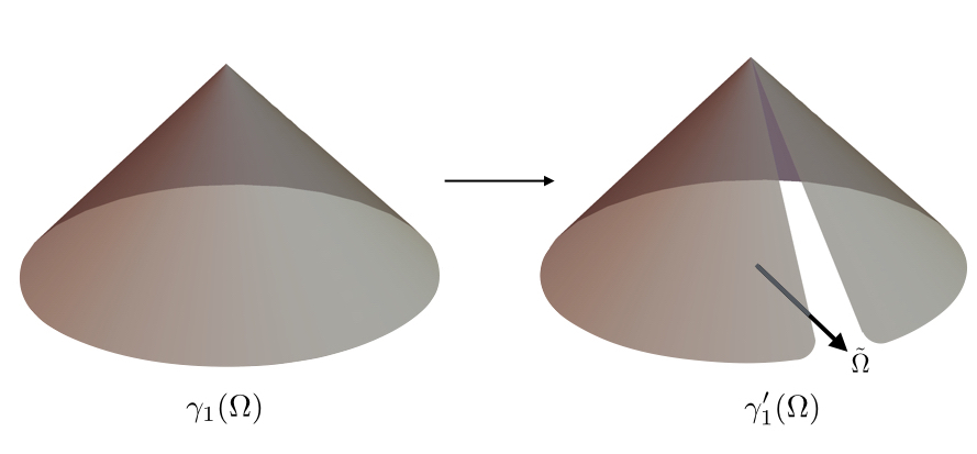
Therefore, there is a very different behaviour of the mutual information as a function of $\gamma_{1}$ for free and non free theories. The continuity of the entropy, or non pinching property, gives a definition of what is a free model from the point of view of the entanglement entropy. Notice that this is not exactly the same as the definition of free theory in terms of Wick’s theorem for correlators. This latter applies for example to generalized free scalar fields with dimension $\Delta>(d-2)/2$ and in this case we expect the pinching property to hold.

We will show that when $k=0,\Delta=(d-2)/2$ or $k=1,\Delta=(d-1)/2$ the mutual information is continuous under pinching on the null cone and the theory has to be free. For higher values of $k\geq 2$ again the saturation is associated to free fields but we discuss these cases later. For $k\geq 2$ and $\Delta=(d+k-2)/2$ the inequality (2.30) actually does not saturate and other terms with smaller $k$ have to appear with the same scaling $\Delta$ for the saturation of strong superadditivity to take place.

Let us then consider $k=0,\Delta=(d-2)/2$ or $k=1,\Delta=(d-1)/2$. Inserting these values in the inequality (2.31) (the non-infinitesimal inequality) it is the result of a direct calculation that it saturates exactly. As the inequality is the result of applying strong superadditivity many times for boosted and rotated spheres, it follows that the saturation of the final inequality implies the saturation of each of the intermediate instances where strong superadditivity was applied. In particular, strong superadditivity for the mutual information with just two boosted spheres must saturate. These spheres can be of any size and boost parameter. The following reasoning shows that this saturation implies in turn the saturation of strong superadditivity for any two surfaces $\gamma_{a}$, $\gamma_{b}$, on the light cone. We are only considering the long distance leading term.

Let us consider the mutual information $I(A,B)$ with $B$ fixed and different $A$’s on a null cone. Strong superadditivity is

	$\displaystyle F(A_{1},A_{2})$	$\displaystyle=$	$\displaystyle I(A_{1}\cap A_{2},B)+I(A_{1}\cup A_{2},B)-I(A_{1},B)-I(A_{2},B)$		(2.43)
		$\displaystyle=$	$\displaystyle S(A_{1}B)+S(A_{2}B)-S((A_{1}\cap A_{2})B)-S((A_{1}\cup A_{2})B)\geq 0\,.$

If we keep the intersection $A_{1}\cap A_{2}$ fixed, this quantity is decreasing with decreasing $A_{1}$ or $A_{2}$ by strong subadditivity. Therefore, if $F(A_{1},A_{2})=0$, the same holds for smaller regions with the same intersection. In the same way (2.43) is decreasing with increasing $A_{1}$ or $A_{2}$ keeping the union $A_{1}\cup A_{2}$ fixed. Therefore, if $F(A_{1},A_{2})=0$, the same holds for bigger regions with the same union. Applying these two rules we get that $F(\gamma_{a},\gamma_{b})=0$ for any intermediate regions $\gamma_{a},\gamma_{b}$ such that $A_{1}\cap A_{2}\subset\gamma_{a},\gamma_{b}\subset A_{1}\cup A_{2}$, and $\gamma_{b}\cap A_{1}\subset\gamma_{a}\cap A_{1}$, $\gamma_{a}\cap A_{2}\subset\gamma_{b}\cap A_{2}$. Given that we can choose spheres $A_{1}$, $A_{2}$ (with the same radius) arbitrarily, it is not difficult to see that we have $F(\gamma_{a},\gamma_{b})=0$ for any regions in the light cone.

Therefore, in analogy with the case of saturation of strong subadditivity of the entropy, we can say that in this situation the mutual information $I(\gamma,B)$ (in the long distance limit) is Markovian with respect to the surface $\gamma$ in the light cone

$$I(\gamma_{1}\cap\gamma_{2},B)+I(\gamma_{1}\cup\gamma_{2},B)-I(\gamma_{1},B)-I(\gamma_{2},B)=0\,.$$

(2.44)

This implies $I(\gamma,B)$ is a local functional of $\gamma(\Omega)$ [16], i.e. an integral

$$I(\gamma,B)=\int d\Omega\,f(\gamma(\Omega),B)\,.$$

(2.45)

This directly implies the mutual information is non-pinching in the above sense. The model then has to contain a free field. We will see the cases $k=0$ or $k=1$ precisely correspond to free scalars and fermions respectively, and we will discuss in more detail the interpretation of $k>1$.

Away from the long distance limit the mutual information for free fields is of course non-pinching, but the inequality does not saturate any more. This is because of the contribution of polynomials of the free fields, as explained in the next sections.

We follow [1] to write the coefficient of the mutual information for well separated regions. The Renyi entropies of integer index are given by expectation values of twist operators in an $n$ replicated theory [23]. That is,

$${\rm tr}\rho_{A}^{n}=\langle\Sigma_{A}^{(n)}\rangle\,,$$

(3.1)

where some regularization is assumed, which is equivalent to a small smearing of the operator $\Sigma_{A}^{(n)}$. This relation was originally thought in Euclidean time but also holds in real time for arbitrary space-like regions [24]. The operator $\Sigma_{A}^{(n)}$ is just the twist (the operator that implements a symmetry locally) of the replicated theory corresponding to the symmetry of cyclic permutation of copies. This symmetry is evidently unbroken in the replicated model. The twist operator transforms fields in the causal development of $A$ and commutes with the operators in the causal complement $A^{\prime}$. The expectation value of the right hand side of (3.1) is on the product state of the vacuum in each of the $n$ copies (or any other state formed by products of the same state in the different copies). For two disjoint regions $A$, $B$, we have

$${\rm tr}\rho_{AB}^{n}=\langle\Sigma_{A}^{(n)}\Sigma_{B}^{(n)}\rangle\,.$$

(3.2)

Then, the idea of [1] is to replace each twist operator in this expression by an operator product expansion (OPE) in terms of field operators in each copy to obtain a series expansion of the mutual information for long distances. The OPE can be written

$$\Sigma^{(n)}_{A}={\rm tr}\rho_{A}^{n}\,\sum_{\{k_{j}\}}C^{A\,\alpha_{0}\ldots\alpha_{n-1}}_{\{k_{j}\}}\,\prod_{j=0}^{n-1}\phi_{k_{j}}^{\alpha_{j}}(r_{A}^{j})\,.$$

(3.3)

The pre-factor ${\rm tr}\rho^{n}_{A}$ is a normalization such that the first coefficient of the expansion corresponding to the identity operator is one, $C_{1}^{A}=1$. Each of the operators $\phi^{\alpha_{j}}_{k_{j}}$ belongs to the $j^{th}$ copy, $k_{j}$ determines the type of field operator and $\alpha_{j}$ is a possible spin index. $r_{A}^{j}$ is a point inside $A$ in the copy $j$.

The Renyi entropy is $S_{n}(A)=(1-n)^{-1}\textrm{tr}(\rho_{A}^{n})$, and the Renyi mutual information

$$I_{n}(A,B)=S_{n}(A)+S_{n}(B)-S_{n}(AB)=\frac{1}{1-n}\log\left(\frac{{\rm tr}\rho_{A}^{n}\,{\rm tr}\rho_{B}^{n}}{{\rm tr}\rho_{AB}^{n}}\right)\,.$$

(3.4)

In the long distance limit this is dominated by the operator of smallest dimension in the OPE expansion. The mutual information is obtained in the limit $n\rightarrow 1$. The leading term of the mutual information is dominated by two copies of the smallest dimension operator in the theory, each one in a different replica.⁶⁶ 6 The contribution to the mutual information of only one operator in one copy vanishes because the coefficient of the one copy operators in the expansion should have a factor $n-1$, such that $\lim_{n\rightarrow 1}\Sigma_{A}^{(n)}=1$, see [2]. One then gets for the leading term

	$\displaystyle I(A,B)$	$\displaystyle\sim$	$\displaystyle\lim_{n\rightarrow 1}\left(\frac{n}{2(n-1)}\sum_{j=1}^{n-1}C_{0j}^{A,\alpha\alpha^{\prime}}C_{0j}^{B,\beta\beta^{\prime}}\right)G_{\alpha\beta}(r_{A},r_{B})G_{\alpha^{\prime}\beta^{\prime}}(r_{A},r_{B})$		(3.5)
		$\displaystyle=$	$\displaystyle D_{A,B}^{\alpha\alpha^{\prime},\,\beta,\beta^{\prime}}G_{\alpha\beta}(r_{A},r_{B})G_{\alpha^{\prime}\beta^{\prime}}(r_{A},r_{B})\,,$

where

$$G_{\alpha\beta}(r_{A},r_{B})=\langle 0|\phi^{\alpha}(r_{A})\,\phi^{\beta}(r_{B})|0\rangle\,.$$

(3.6)

If the operators in the two copies are complex there is an additional factor $2$ in (3.5).

Calling $\Delta$ to the dimension of the lowest dimension operator, (3.5) falls as $L^{-4\Delta}$. The coefficients could in principle be obtained from (3.3) taking correlators with fields at large space-like distances

$$C^{A\alpha\alpha^{\prime}}_{0j}G_{\alpha\gamma}(r_{A},r)G_{\alpha^{\prime}\gamma^{\prime}}(r_{A},r)=\frac{\langle\Sigma_{A}^{(n)}\phi_{0}^{\gamma}(r)\phi_{j}^{\gamma^{\prime}}(r)\rangle}{{\rm tr}\rho_{A}^{n}}\,,\hskip 28.45274ptr^{2}\rightarrow\infty\,.$$

(3.7)

In order to better understand this coefficient we recall that (in presence of a regulator) the Hilbert space can be decomposed as ${\cal H}_{A}\otimes{\cal H}_{A^{\prime}}$ for the region $A$, where $A^{\prime}$ is the complementary region. Then we can write a tensor product basis for the Hilbert space on each copy as $\{|e^{i}_{a},f^{i}_{b}\rangle\}$, where $i$ is the index of copies and $a,b$ the ones spanning the basis for each copy. Then we can write the twist operator in explicit form [24]

$$\Sigma_{A}^{(n)}=\bigotimes_{i=0}^{n-1}\left(\sum_{a}|e^{i+1}_{a}\rangle\langle e^{i}_{a}|\right)\otimes 1_{{\cal H}_{A^{\prime}}}\,,$$

(3.8)

with cyclic notation $|e^{n}_{a}\rangle\equiv|e^{0}_{a}\rangle$. This operator is unitary and does not depend on the chosen basis. If $|0^{i}\rangle$ is the global state in the copy $i$, and $|\Omega\rangle=\otimes_{i}|0^{i}\rangle$, it is not difficult to show using the Schmidt decomposition for $|0^{i}\rangle$ in ${\cal H}_{A}^{i}\otimes{\cal H}_{A^{\prime}}^{i}$, that

	$\displaystyle\langle\Omega|\Sigma_{A}^{(n)}|\Omega\rangle$	$\displaystyle=$	$\displaystyle{\rm tr}\rho_{A}^{n}\,,$
	$\displaystyle\langle\Omega|\Sigma_{A}^{(n)}\,{\cal O}^{A,j}|\Omega\rangle$	$\displaystyle=$	$\displaystyle{\rm tr}(\rho_{A}^{n}\,{\cal O}^{A})\,,$		(3.9)
	$\displaystyle\langle\Omega|\Sigma_{A}^{(n)}\,{\cal O}_{1}^{A,j}\,{\cal O}_{2}^{A,j^{\prime}}|\Omega\rangle$	$\displaystyle=$	$\displaystyle{\rm tr}(\,{\cal O}_{1}^{A}\,\rho_{A}^{n-(j-j^{\prime})}\,{\cal O}_{2}^{A}\,\rho_{A}^{(j-j^{\prime})})\,,$

where ${\cal O}^{A}$ is an operator in $A$ in the original single copy space, and ${\cal O}^{A,j}$ is its representative in the $j^{th}$ copy. In the right hand side of these formulas we have expressions in a single copy Hilbert space. We also have

$$\Sigma_{A^{\prime}}^{(n)}\Sigma_{A}^{(n)}|\Omega\rangle=|\Omega\rangle\,,\hskip 28.45274pt\Sigma_{A}^{(n)}|\Omega\rangle=(\Sigma_{A^{\prime}}^{(n)})^{-1}|\Omega\rangle\,,$$

(3.10)

where $(\Sigma_{A^{\prime}}^{(n)})^{-1}$ just changes the order of copies with respect to $\Sigma_{A^{\prime}}^{(n)}$.

Therefore, the right hand side of (3.7), where the operators live in $A^{\prime}$, amounts to evaluate

$$\frac{{\rm tr}(\rho_{A^{\prime}}^{n}\,\rho_{A^{\prime}}^{-j}\phi^{\gamma}(r)\,\rho_{A^{\prime}}^{j}\,\phi^{\gamma^{\prime}}(r))}{{\rm tr}\rho_{A}^{n}}=\frac{{\rm tr}(\rho_{A^{\prime}}^{n}\,\phi_{A}^{\gamma}(r,\tau=ij)\,\phi^{\gamma^{\prime}}(r))}{{\rm tr}\rho_{A}^{n}}$$

(3.11)

where all operators are in a single copy theory, and

$$\phi_{A}^{\gamma}(r,\tau)=\rho_{A^{\prime}}^{i\tau}\phi^{\gamma}(r)\rho_{A^{\prime}}^{-i\tau}$$

(3.12)

is the field transformed by the modular flow of $A^{\prime}$, which coincides, except for the sign of $\tau$, with the modular flow of $A$ (and this is why we have called it with subscript $A$).

References

- [1] J. Cardy, “Some results on the mutual information of disjoint regions in higher dimensions,” Journal of Physics A: Mathematical and Theoretical 46 no. 28, (2013) 285402. http://stacks.iop.org/1751-8121/46/i=28/a=285402.
- [2] C. A. Agón and T. Faulkner, “Quantum corrections to holographic mutual information,” Journal of High Energy Physics 2016 no. 8, (2016) 118.
- [3] B. Chen and J.-J. Zhang, “On short interval expansion of Rényi entropy,” JHEP 11 (2013) 164, arXiv:1309.5453 [hep-th].
- [4] M. Headrick, “Entanglement Renyi entropies in holographic theories,” Phys. Rev. D82 (2010) 126010, arXiv:1006.0047 [hep-th].
- [5] P. Calabrese, J. Cardy, and E. Tonni, “Entanglement entropy of two disjoint intervals in conformal field theory,” J. Stat. Mech. 0911 (2009) P11001, arXiv:0905.2069 [hep-th].
- [6] P. Calabrese, J. Cardy, and E. Tonni, “Entanglement entropy of two disjoint intervals in conformal field theory II,” J. Stat. Mech. 1101 (2011) P01021, arXiv:1011.5482 [hep-th].
- [7] M. A. Rajabpour and F. Gliozzi, “Entanglement Entropy of Two Disjoint Intervals from Fusion Algebra of Twist Fields,” J. Stat. Mech. 1202 (2012) P02016, arXiv:1112.1225 [hep-th].
- [8] J. Long, “On co-dimension two defect operators,” arXiv:1611.02485 [hep-th].
- [9] B. Chen, L. Chen, P.-x. Hao, and J. Long, “On the mutual information in conformal field theory,” Journal of High Energy Physics 2017 no. 6, (2017) 96.
- [10] C. A. Agon, I. Cohen-Abbo, and H. J. Schnitzer, “Large distance expansion of Mutual Information for disjoint disks in a free scalar theory,” JHEP 11 (2016) 073, arXiv:1505.03757 [hep-th].
- [11] B. Chen and J. Long, “Rényi mutual information for a free scalar field in even dimensions,” Phys. Rev. D96 no. 4, (2017) 045006, arXiv:1612.00114 [hep-th].
- [12] H. J. Schnitzer, “Mutual Rényi information for two disjoint compound systems,” arXiv:1406.1161 [hep-th].
- [13] H. Casini and M. Huerta, “On the RG running of the entanglement entropy of a circle,” Phys. Rev. D85 (2012) 125016, arXiv:1202.5650 [hep-th].
- [14] H. Casini, E. Testé, and G. Torroba, “Modular hamiltonians on the null plane and the markov property of the vacuum state,” Journal of Physics A: Mathematical and Theoretical 50 no. 36, (2017) 364001.
- [15] H. Casini, E. Testé, and G. Torroba, “Markov property of the conformal field theory vacuum and the a theorem,” Physical review letters 118 no. 26, (2017) 261602.
- [16] H. Casini, E. Testé, and G. Torroba, “All the entropies on the light-cone,” Journal of High Energy Physics 2018 no. 5, (2018) 5.
- [17] P. H. Ginsparg, “Applied conformal field theory,” arXiv:hep-th/9108028.
- [18] H. Casini and M. Huerta, “A Finite entanglement entropy and the c-theorem,” Phys. Lett. B600 (2004) 142–150, arXiv:hep-th/0405111 [hep-th].
- [19] S. Minwalla, “Restrictions imposed by superconformal invariance on quantum field theories,” Adv. Theor. Math. Phys. 2 (1998) 783–851, arXiv:hep-th/9712074.
- [20] S. Schlieder and E. Seiler, “Some remarks on the “null plane development” of a relativistic quantum field theory,” Communications in Mathematical Physics 25 no. 1, (1972) 62–72.
- [21] A. C. Wall, “A proof of the generalized second law for rapidly changing fields and arbitrary horizon slices,” Phys. Rev. D85 (2012) 104049, arXiv:1105.3445 [gr-qc]. [Erratum: Phys. Rev.D87,no.6,069904(2013)].
- [22] R. Bousso, H. Casini, Z. Fisher, and J. Maldacena, “Entropy on a null surface for interacting quantum field theories and the Bousso bound,” Phys. Rev. D91 no. 8, (2015) 084030, arXiv:1406.4545 [hep-th].
- [23] P. Calabrese and J. Cardy, “Entanglement entropy and quantum field theory,” Journal of Statistical Mechanics: Theory and Experiment 2004 no. 06, (2004) P06002.
- [24] H. Casini and M. Huerta, “Positivity, entanglement entropy, and minimal surfaces,” Journal of High Energy Physics 2012 no. 11, (2012) 87.
- [25] R. Haag, Local quantum physics: Fields, particles, algebras. 1992.
- [26] C. P. Herzog, “Universal Thermal Corrections to Entanglement Entropy for Conformal Field Theories on Spheres,” JHEP 10 (2014) 28, arXiv:1407.1358 [hep-th].
- [27] K. Alkalaev, “Mixed-symmetry tensor conserved currents and AdS/CFT correspondence,” J. Phys. A 46 (2013) 214007, arXiv:1207.1079 [hep-th].
- [28] M. S. Costa and T. Hansen, “Conformal correlators of mixed-symmetry tensors,” JHEP 02 (2015) 151, arXiv:1411.7351 [hep-th].
- [29] T. Hirai, “The characters of irreducible representations of the lorentz group of n-th order,” Proceedings of the Japan Academy 41 no. 7, (1965) 526–531.
- [30] G. Mack, “All unitary ray representations of the conformal group SU(2,2) with positive energy,” Commun. Math. Phys. 55 (1977) 1.
- [31] W. Siegel, “All Free Conformal Representations in All Dimensions,” Int. J. Mod. Phys. A 4 (1989) 2015.
- [32] P. S. Howe, S. Penati, M. Pernici, and P. K. Townsend, “A Particle Mechanics Description of Antisymmetric Tensor Fields,” Class. Quant. Grav. 6 (1989) 1125.
- [33] F. A. Dolan and H. Osborn, “Conformal Partial Waves: Further Mathematical Results,” arXiv:1108.6194 [hep-th].
- [34] M. S. Costa, J. Penedones, D. Poland, and S. Rychkov, “Spinning Conformal Blocks,” JHEP 11 (2011) 154, arXiv:1109.6321 [hep-th].