Kepler’s Goat Herd: An Exact Solution to Kepler’s Equation for Elliptical Orbits2021Kepler’s Goat Herd: An Exact Solution to Kepler’s Equation for Elliptical Orbits–References

Kepler’s equation states that

for eccentric anomaly $E\in[0,2\pi)$, eccentricity $e\in[0,\infty)$ and mean anomaly $\ell\in[0,2\pi)$ (often denoted $M$). This describes the dynamics of a two-body system, and was first published over 400 years ago (Kepler 1609). It is most commonly applied to (non-circular) elliptical orbits, whereupon $0<e<1$. Assuming such an orbit, the quantities in (1) may be related to other orbital parameters of interest via

(Murray & Dermott 1999), with $t-\tau$ being the time-coordinate relative to pericenter crossing, $n$ the mean motion, $a$ the semi-major axis, and $(x,y)$ the Cartesian positions in the orbital plane, relative to the center of the ellipse. A solution of (1) thus specifies the full location of the orbiting body as a function of time.

Despite its age, Kepler’s equation is no less relevant today than in 1609; it still appears in many contexts, with crucial examples including Global Positioning System (GPS) calibration and the determination of satellite and debris positions by the United States Space Surveillance Network (SSN)¹¹ 1 See www.space-track.org.. Being a transcendental equation, conventional methods cannot solve (1) directly, which has led to a vast literature concerning alternative approaches, such as root-finding and series solutions. Indeed, Colwell 1993 notes that new methods of solution have been proposed in almost every decade since 1650. Below, we present our contribution to this canon.

Before discussing Kepler’s equation in detail, we briefly mention a seemingly unrelated topic: the ‘geometric goat problem’. Roughly speaking, the problem is the following: "Imagine a goat is tied to the edge of a circular enclosure. How long must the rope be such that the goat can graze in exactly half of the field?" Recent work by Ullisch 2020 shows this to be equivalent to solving the transcendental equation $\sin\beta-\beta\cos\beta=\pi/2$ for $\beta$. Using methods drawn from complex analysis, Ullisch 2020 provides an explicit solution to the problem via a ratio of contour integrals, each of which can be easily computed using FFTs or direct summation. Given the similarity between this and (1), we may ask whether an analogous solution is possible in our case. Further support for this approach is given by Slepian & Philcox 2021, which used the same methods to explicitly solve the spherical collapse equations, which are a special case of (1) with $e=1$.

The remainder of this paper is structured as follows. In §2 we present the explicit solution of Kepler’s equation, alongside a proof of its validity, before discussing its practical evaluation in §3. Discussion of alternative solution methods is provided in §4 before a comparison is made in §5 alongside our conclusions. All computations in this work were performed in C++ and plotted using python.

Our first step is to demonstrate that (1) has a unique solution in the range of interest. We will assume that the eccentricity is both fixed and in the range $e\in(0,1)$, i.e. that we have a non-circular elliptical orbit. Considering the function

the solution $E^{*}(\ell,e)$ satisfies $g(E_{*}(\ell,e);e)=\ell$. Given that $g(E;e)$ is an odd function of $e$, and (1) is invariant under $E\to E+2\pi$, $\ell\to\ell+2\pi$, we need only consider the range $\ell\in[0,\pi]$. We additionally avoid the trivial solutions $E=0,\pi$ at $\ell=0,\pi$.

Considering the end-points, $g(0;e)=0$, $g(\pi;e)=\pi$; since the function is smooth, $g(E;\ell,e)$ must thus equal $\ell$ at least once for all $\ell\in(0,\pi)$. In fact $g(E;e)$ is monotonic in $E$ for all $|e|<1$, hence there is a single solution $E_{*}(\ell,e)$. This is easily shown by noting that both $E$ and $e\sin E$ are zero at $E=0$ and $E$ increases faster than $|e\sin E|$ for all $|e|<1$, hence $E>|e\sin E|$ everywhere. For reference, we provide a plot of the solution $E_{*}(\ell,e)$ for various values of $e$ and $\ell$ in Fig. 1.

To define an integral solution to (1), we first consider the entire function $f$

defined on a simply-connected region $U=(0,2\pi)\times i(-\infty,\infty)$ in the complex plane. The parameters $e,\ell$ take the values $e\in(0,1)$ and $\ell\in(0,\pi)$ as before. Restricting to the real line, the solution to $f(z;\ell,e)=0$, denoted $z_{0}(\ell,e)$, recovers Kepler’s equation, in the sense that $z_{0}(\ell,e)\equiv E_{*}(\ell,e)$.

To proceed, we use the theorem of Ullisch 2020, as in Slepian & Philcox 2021 (and found previously in Jackson 1916; Jackson 1917; Luck & Stevens 2002; Luck et al. 2015).²² 2 An alternative solution using complex methods can be found in Siewert & Burniston 1972. Our approach is significantly more straightforward however. This states that, for an open simply connected subset $U$ of $\mathbb{C}$ with a non-zero analytic function $f$ defined therein, for each simple zero $z_{0}\in U$ of $f$, there exists a closed curve $C\in U$ such that:

(5) follows directly from the Residue Theorem under the assumptions stated: the numerator evaluates to $2\pi iz_{0}/f^{\prime}(z_{0})$, and the denominator to $2\pi i/f\textquoteright(z_{0})$. Furthermore, (5) holds for any Jordan curve $C\in U$, provided that (a) it encloses $z_{0}$, and (b) $f(z)\neq 0$ at all points on $C$ and its interior, except at $z=z_{0}$.

In our context, $f(z)\equiv f(z,\ell,e)$ is defined by (4), and, provided certain conditions are met, we may use (5) to evaluate $z_{0}(\ell,e)$ and hence obtain $E_{*}(\ell,z)$. Below, we consider the conditions in detail:

1. 1.

   $z_{0}$ lies within $U$. By the discussion above, $f(z,\ell,e)=0$ on the real-line at a single point with $z_{0}(\ell,e)=E_{*}(\ell,e)$. Since $E\in(0,\pi)$ (for $\ell\in(0,\pi)$), $z_{0}$ lies within $U$.

2. 2.

   $z_{0}$ is a simple zero. From (4), $f^{\prime}(z)=1-e\cos z$, which, for $e\in(0,1)$, has no solutions on the real line. Thus $f^{\prime}(z_{0})\neq 0$, hence the zero at $z_{0}$ is simple.

3. 3.

   $z_{0}$ is enclosed within $C$. A simple choice is to assume the (Jordan) circular contour $C=\{z:|z-\pi/2|<\pi/2-\epsilon\}$ for small parameter $\epsilon>0$ (analogous to Slepian & Philcox 2021). This intersects the real axis at $\mathrm{Re}[z]=\epsilon,\pi-\epsilon$; thus, for sufficiently small $\epsilon$, $z_{0}$ is enclosed with $C$ (for any choice of $e$ and $\ell$). In practice, we find a different contour to be more advantageous for efficient numerical implementation; this is discussed below.

4. 4.

   $z_{0}$ is the only zero within $C$. To prove this, we first consider the region $\mathcal{R}\subset U$ defined by $\mathcal{R}=(0,2\pi)\times i(-M,M)$ for large $M$. Since $C$ lies within $\mathcal{R}$, the condition is satisfied if $f(z;\ell,e)\neq 0$ everywhere in $\mathcal{R}\backslash\{z_{0}\}$.³³ 3 The notation $\mathcal{R}\backslash\{z_{0}\}$ indicates the set $\mathcal{R}$ excluding the point $z_{0}$. To prove this, we consider the variation in $\mathrm{arg}[f(z;\ell,e)]$ as one traverses the boundary $\partial\mathcal{R}$ in a counter-clockwise fashion. Writing $z=(x+iy)$, $f(z;\ell,e)$ may be written $f(x,y;\ell,e)=\left(x-e\sin x\cosh y-\ell\right)+i\left(y-e\cos x\sinh y\right)$. Considering each part of the contour in turn, and taking $M\to\infty$:

   • •

     Moving from $z=0-iM$ to $z=2\pi-iM$, we have $f(z;\ell,e)=(i/2)e\exp(M+ix)+\mathcal{O}(M)$, thus $\Delta\mathrm{arg}\left[f(z;\ell,e)\right]=+2\pi$.

   • •

     From $z=2\pi-iM$ to $2\pi+iM$, $f(z;\ell,e)=2\pi-\ell+i(y-e\sinh y)$, thus $\mathrm{Re}[f(z;\ell,e)]$ is constant and positive, whilst $\mathrm{Im}[f(z;\ell,e)]$ moves from $(1/2)e\exp{M}$ to $-(1/2)e\exp M$, giving $\Delta\mathrm{arg}\left[f(z;\ell,e)\right]=-\pi$.

   • •

     Similarly from $z=2\pi+iM$ to $0+iM$, $f(z;\ell,e)=-(i/2)e\exp(M-ix)+\mathcal{O}(M)$, thus $\Delta\mathrm{arg}[f(z;\ell,e)]=+2\pi$.

   • •

     Finally, from $z=0+iM$ to $z=0-iM$, $f(z;\ell,e)=-\ell+i(y-e\sinh y)$, thus $\mathrm{Re}[f(z;\ell,e)]$ is constant and negative, whilst $\mathrm{Im}[f(z;\ell,e)]$ moves from $-(1/2)e\exp M$ to $(1/2)e\exp M$, giving $\Delta\mathrm{arg}\left[f(z;\ell,e)\right]=-\pi$.

   Summing the contributions, we find $\Delta\mathrm{arg}[f(z;\ell,e)]=+2\pi$ when traversing the full closed contour $\partial\mathcal{R}$ in a counter-clockwise fashion. From the argument principle, this is equal to $2\pi(Z-P)$ where $Z$ and $P$ are respectively the number of zeros and poles within $\mathcal{R}$. Since $P=0$ (as neither $z$ nor $\sin z$ contain any poles in $\mathbb{C}$), we find $Z=1$, thus $\mathcal{R}$ contains only a single zero. This implies that $z_{0}$ is the only zero of $f(z;\ell,e)$ in $\mathcal{R}$, or, given that $M$ is arbitrary, $f(z;\ell,e)\neq 0$ for all $z\in U\backslash\{z_{0}\}$.

It remains to choose the contour $C$. Whilst the large circle $C=\{z:|z-\pi/2|<\pi/2-\epsilon\}$ is a valid choice, given that it lies within $U$ and encloses $z_{0}$, for numerical efficiency it is preferred to use a smaller circular contour (cf. §3). To form this, we first consider the function $g(E;e)=E-e\sin E$ (cf. 3) in more detail. In particular, we note that for $E\in(0,\pi)$:

Given that our solution requires $g(E^{*}(\ell,e);e)=\ell$, we find the bound $E_{*}(\ell,e)\in(\ell,\ell+e)$ for $\ell<\pi$, as shown in Fig. 1. Together, this motivates the contour $C=\{z:|z-(\ell+e/2)|=e/2\}$, i.e. a circle of radius $e/2$ centered at $\ell+e/2$. This is guaranteed to enclose $z_{0}$ (ignoring the trivial case $\ell=\pi$), and is contained within $U$, since $e<\pi/2$.⁴⁴ 4 An alternative bound is given by $E_{*}(\ell,e)\in(\ell,\mathrm{min}[\pi,\ell+e])$. Whilst this results in a tighter contour for $\ell>\pi-e$, it will not be applied in this work, since the associated circular contour has a radius dependent on $\ell$, which hampers numerical efficiency (cf. §3), since the contour integrand is no longer separable in $\ell$ and the path-variable $x$. For further discussion on solution bounds see Serafin 1986; Serafin 1998.

Given the above, we may apply (5) to our problem, obtaining the solution

This may be straightforwardly inserted into (2) to obtain the Cartesian evolution of the orbit as a function of $\ell$. For reference, we show the function $f(z;\ell,e)$ alongside the region $U$ and the contour $C$ in Fig. 2, for a representative choice of $\ell$ and $e$.

To obtain a simply implementable form of (7), we first parametrize the circular contour $C$ by the function $\gamma:[0,1)\rightarrow C$ where $\gamma(x)=x_{0}+\Delta x\,e^{2\pi ix}$ for contour center $x_{0}$ and radius $\Delta x$. As in §2, these are set to $x_{0}=\ell+e/2$, $\Delta x=e/2$. Inserting this into (7) and changing variables leads to

where we define

Defining the Fourier series coefficients of $a(x;\ell,e)$ by

for integer $k$, (8) can be written

For any given $\ell$ or $e$, we can thus evaluate $E_{\ast}(\ell,e)$ by computing the integrals $a_{-2}$ and $a_{-1}$. In general, these must be evaluated numerically. One option for this (advocated for in Ullisch 2020 and Slepian & Philcox 2021) is to use a Fast Fourier Transform (FFT) to obtain all $a_{k}$ frequencies simultaneously, for given $\ell,e$. However, this is not the most efficient choice. The FFT algorithm scales as $N\log N$, for $N$ grid-points; for computing $N$ frequencies, this is clearly superior to computing $N$ numerical integrals, but when only two are required (as here), the latter method is preferred. To expedite computation, we note that the real-part of each integral is symmetric around $x=0.5$ (with the imaginary part antisymmetric, and thus cancelling), giving

where we have approximated the integral by a discrete sum of $N$ points in the second line, for some normalization constant $A$ which will cancel in (11) when we take the ratio. Furthermore, we may compute the real parts explicitly and thus avoid any invoking complex numbers in the implementation of (12), again leading to faster computation. Alternative numerical methods such as Goertzel’s algorithm (Goertzel 1958) may also be used to approximate these integrals.

From (11), we see the utility of using a narrow contour $C$. If $\Delta x$ is small (implying $x_{0}$ is close to the true solution, since the latter must be enclosed by $C$), then the second term of (11) must also be small. For a given desired accuracy in $E_{*}$ one can thus use fewer grid-points $N$ for the numerical integral in (12), obtaining a faster algorithm. This is borne out in practice, since the contour with $x_{0}=\ell+e$ and $\Delta x=\pi/2$ is found to be much more accurate than $x_{0}=\pi/2$, $\Delta x=\pi/2-\epsilon$ (the analog to that used in Slepian & Philcox 2021) for the same $N$.

In a typical setting, one may wish to compute the eccentric anomaly $E_{*}(\ell,e)$ for many values of $\ell$ (equivalently, time) simultaneously. In this case, computation can be expedited by pre-computing $\sin(-2\pi ikj)$ (which is independent of $\ell$) for each $j=1,...,N-1$. Additionally, the factor $\sin\left(x_{0}+\Delta x\,e^{2\pi ix}\right)$ appearing in (9) may be expanded as

Whilst elementary, this is nonetheless useful. With our choice of contour, $x_{0}\equiv x_{0}(\ell,e)$, $\Delta x\equiv\Delta x(e)$, with neither depending on $x$. This implies that the factors $\sin x_{0}$, $\cos x_{0}$ are independent of $x$ (and hence $N$), thus must be computed only once per integral evaluation. Since $\Delta x$ is independent of $\ell$, every other function appearing in (13) needs to be computed only once per sampling point, even if a large array is used. This reduces the number of trigonometric function evaluations from $N_{\ell}\times(N-1)$ to $N_{\ell}+N-1$ , where $N_{\ell}$ is the size of the input $\ell$ array, and we note that the points $x=0$ and $x=0.5$ are trivial. Once the functions appearing in (13) are precomputed, (12) requires only addition and multiplication operations, thus is highly efficient.

Before presenting the results of our approach, we discuss several popular alternatives. Further details on these can be found in Murray & Dermott 1999 and Danby 1988.

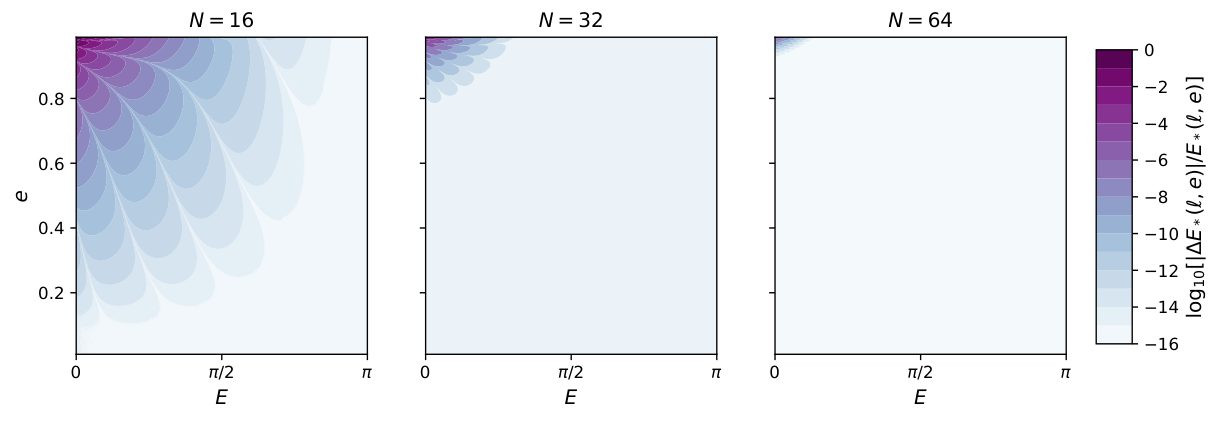
We now compare our prescription (§2 & §3) to the well-known techniques of §4. For testing, we generate a grid of $10^{6}$ equally-spaced points in eccentric anomaly $E$ (defining the ‘ground truth’ solution) and compute the mean anomaly $\ell$ for each via (1), assuming $e$ to be fixed. Figs. 3 compares the results from our method (using $10^{3}$ grid-points) with the truth for two choices of eccentricity $e$ and various numbers of grid-points, $N$. The results are as expected: the error in the approach falls strongly with increasing $N$,⁵⁵ 5 The error decreases exponentially with increasing $N$ at fixed $e$ because the error is due to aliasing of higher-frequency Fourier harmonics, and because harmonics of analytic functions fall exponentially at rates proportional to the distance from the integration contour to the nearest singularity. with accuracy of machine precision achieved for most $\ell$ at $N=8$ ($N=16$) for $e=0.3$ ($e=0.9$). Furthermore, we find a generally larger error at higher $e$: this is expected since the radius of the integration contour is proportional to $e$, and the solutions lie further from the line $E=\ell$, as in Fig. 1. This is further explored in Fig. 4, whereupon the error is shown to increase as one moves towards the singularity at $e=1$, $\ell=0$. Increasing the number of grid-points greatly reduces this however, highlighting the importance of choosing $N$ appropriately.

To place our method in context, we compare it to the three alternative prescriptions (series, Newton-Raphson, and Danby) discussed in §4. For this purpose, we implement each in C++, paying close attention to efficiency.⁶⁶ 6 C++ code implementing all of these can be found at github.com/oliverphilcox/Keplers-Goat-Herd. To ensure each method has a similar level of accuracy, we gradually increase the precision of each method (either by increasing the number of grid-points in the numerical integral, or the number of iterations) until a mean absolute precision of $10^{-12}$ is obtained relative to the ‘ground-truth’ solution.

The final hyperparameter values and runtimes for the $N_{\ell}=10^{6}$ array of mean anomalies are shown in Tab. 1 for three values of the eccentricity. As expected, both the Newton-Raphson and Danby methods converge quickly, with the latter requiring a maximum of three iterations even at the most extreme case of $e=0.9$. The Danby prescription requires more computational operations per iteration, thus its runtime is only slightly reduced relative to Newton-Raphson, despite the fact that the number of iterations is roughly halved. Significantly more iterations are required for the series solution of (14), particularly as $e$ increases. Given its nature as a perturbative solution, this is unsurprising, and we conclude that it is of most use only for orbits of very low eccentricity. Finally, we consider our approach. In all cases, we require $N\leq 18$ grid-points in the numerical integral (with $N$ rising as $e$ increases, as in Fig. 2), and find that the computation time is significantly reduced (by a factor $\sim$ $2-3$) compared to any of the alternative prescriptions. This may be understood by considering the number of trigonometric operations involved: assuming $N_{\ell}\gg N$, the total is proportional to $N_{\ell}$, and thus independent of the number of steps. Each integration step simply requires multiplication and addition operations, giving a faster speed.

To summarize, this work demonstrates that new methods to solve the Kepler equation can provide solutions outperforming those of established methods over a wide range of parameter space. Our approach is based on contour integration, using methods developed to solve the ‘geometric goat problem’ in Ullisch 2020 and recently applied to the dynamics of spherical collapse in Slepian & Philcox 2021. We expect such approaches to be similarly applicable to other problems that require the solution of transcendental equations.

The data underlying this article will be shared on reasonable request to the corresponding author. C++ and python implementations of our code are available at github.com/oliverphilcox/Keplers-Goat-Herd.

We thank Tom Dickens, Hanno Rein, Ian Weaver and the Twitterverse for insightful feedback. We are additionally grateful to the referee, Manuel Calvo, for an insightful report. OP acknowledges funding from the WFIRST program through NNG26PJ30C and NNN12AA01C.

References

- Calvo et al. (2013) Calvo M., Elipe A., Montijano J. I., Rández L., 2013, Celestial Mechanics and Dynamical Astronomy, 115, 143
- Colwell (1993) Colwell P., 1993, Solving Kepler’s equation over three centuries. Willmann-Bell, Richmond, Virginia
- Danby (1987) Danby J. M. A., 1987, Celestial Mechanics, 40, 303
- Danby (1988) Danby J. M. A., 1988, Fundamentals of celestial mechanics. Willmann-Bell, Richmond, Virginia
- Elipe et al. (2017) Elipe A., Montijano J. I., Rández L., Calvo M., 2017, Celestial Mechanics and Dynamical Astronomy, 129, 415
- Goertzel (1958) Goertzel G., 1958, The American Mathematical Monthly, 65, 34
- Hagihara (1970) Hagihara Y., 1970, Celestial mechanics. Vol.1: Dynamical principles and transformation theory. MIT Press
- Jackson (1916) Jackson D., 1916, Ann. of Math., 17, 172
- Jackson (1917) Jackson D., 1917, Ann. of Math., 19, 142
- Kepler (1609) Kepler J., 1609, Astronomia Nova Aitiologētos, Seu Physica Coelestis, tradita commentariis De Motibus Stellæ Martis, Ex observationibus G. V. Tychonis Brahe
- Luck & Stevens (2002) Luck R., Stevens J. W., 2002, SIAM Review, 44, 227
- Luck et al. (2015) Luck R., Zdaniuk G., Cho H., 2015, International Journal of Engineering Mathematics, 523043
- Markley (1995) Markley F. L., 1995, Celestial Mechanics and Dynamical Astronomy, 63, 101
- Murray & Dermott (1999) Murray C. D., Dermott S. F., 1999, Solar system dynamics. Cambridge University Press
- Serafin (1986) Serafin R. A., 1986, Celestial Mechanics, 38, 111
- Serafin (1998) Serafin R. A., 1998, Celestial Mechanics and Dynamical Astronomy, 70, 131
- Siewert & Burniston (1972) Siewert C. E., Burniston E. E., 1972, Celestial Mechanics, 6, 294
- Slepian & Philcox (2021) Slepian Z., Philcox O. H. E., 2021, arXiv e-prints, p. arXiv:2103.09823
- Ullisch (2020) Ullisch I., 2020, The Mathematical Intelligencer, 42, 12