Design of Experiments with Imputable Feature Data: An Entropy-Based Approach

Parametric models are pivotal for analysis, design, control, and optimization in many studies and applications such as textile manufacturing[1], food [2], energy[3] and pharmaceutical[4] industries. Often, the unknown parameters in these models are estimated using experimental data. However, in many of these applications, running experiments are expensive and time-consuming. Therefore, it is very important to carefully select few experiments to be performed while simultaneously ensuring reliable parameter estimation. Model-Based Design of Experiments (DoE)[5] introduces statistical methods which pose and solve appropriate optimization problems that strategically select experiments from a large set of possible experiments. These selection problems are also common in other contexts, for instance, the application areas that use learning tasks such as active learning[6], multi-arm bandits[7], diversity sampling[8] require effective selection of input data.

Linear models of the form $y=f^{\top}(\mathbf{z})\beta$, where the measured output depends linearly on the parameters $\beta$ (not necessarily linear on the process variables $\mathbf{z}$) are very common in many of the above applications. DoE for these linear models is critical since they are extensively used, are amenable to simpler interpretations, and offer tractable solution to the experiment selection problem [9],[10],[11]. The underlying principle for these statistical techniques is to select a small subset from a pre-specified set $\Omega$ of process variables $\{\mathbf{z}_{i}\}_{i=1}^{n}$ at which the experiments need to be conducted to obtain a reasonable estimate $\hat{\beta}$ of $\beta\in\mathbb{R}^{p}$ such that $f^{T}(\mathbf{z})\hat{\beta}$ is a good (low variance) estimation of $y$ for all $\mathbf{z}$ in $\Omega$. More precisely, a case with $r$ experimental observations $\mathbf{y}\in\mathbb{R}^{r}$ at process values $\{\mathbf{z}_{i}\}_{1}^{r}$ ($r\ll n$) can be written as $\mathbf{y}=X\beta+\epsilon$, where $X\in\mathbb{R}^{r\times p}$, $f(\mathbf{z}_{i})^{\top}$ is the $i$th row of $X$, and $\epsilon$ is the error vector (typically assumed to be realizations of independent and identically distributed (iid) random variables).

A least square estimate for this regression problem is given by $\hat{\beta}=(X^{\top}X)^{-1}X^{\top}\mathbf{y}$ and the variance $var(\hat{\beta})=\sigma^{2}(X^{\top}X)^{-1}$, where $\sigma^{2}$ is the variance of $\epsilon$. Also the predicted response is $\hat{}\mathbf{y}(\mathbf{z})=f^{\top}(\mathbf{z})\hat{\beta}$ with variance $var(\hat{}\mathbf{y}(\mathbf{z}))=\sigma^{2}f^{\top}(\mathbf{z})(X^{\top}X)^{-1}f(\mathbf{z})$. The DoE problem deals with choosing an appropriate choice of $r$ process values $\{\mathbf{z}_{i}\}_{i=1}^{r}$ from a larger set $\Omega$, such that the corresponding Fisher information matrix $\Sigma=X^{\top}X$ [12] ensures small variance in predicted response; here $r$ is known a priori and is small enough to be cost and time effective.

In particular, various optimality criteria $g(\Sigma)\in\mathbb{R}$ are used for DoE [5]; for instance $A$-optimality criterion requires parsimonious selection of ${\mathbf{z}_{i}}$ such that $g(\Sigma)=\text{trace}(\Sigma^{-1})$ is minimized (See Figure 1). Other such criteria include D-optimality (minimize $\text{determiniant}(\Sigma^{-1}$), T-optimality (maximize $\text{trace}(\Sigma)$), E-optimality (minimize ${\text{maximum eigenvalue}(\Sigma)}$), V-optimality (minimize average prediction variance), and G-optimality (minimize worst possible prediction variance) [5]. These optimization problems are combinatorial in nature and are known to be NP hard[13].

These problems become even more complex when not all process variable values are preset but need to be chosen or designed. More precisely, in the context of linear regression models considered above, when some elements in the matrix $X$ are themselves parameters to be designed (chosen typically from a continuous domain set). These problems arise in DoE applications where not all process variables $\mathbf{z}_{i}\in\Omega$ are determined a priori, but are free to be chosen. For instance if $y$ represents taste-quality score of a certain wine and $f_{k}(\mathbf{z})$ represents a specific feature (among many other features) – say that depends on temperature of the room at which wine is served; the temperature values can be treated as a design variable. Similar objectives also arise in certain missing-data problems, where values for $f_{k}(\mathbf{z}_{i})$ (for some ($k,i$)) are missing and these values need to be imputed. Missing of data can occur due to various reasons such as unreliable sensors[14], system malfunction[15][16] or incomplete surveys[17]. While range of missing data points are known, exact values might still be missing. This is widespread in many research areas and has adverse affects on final model estimation[18, 19, 20]. The corresponding complexity of DoE problem increases since solving for the above optimality criteria will require solving simultaneously the selection problem as well as designing these parameters.

There are many approaches that address individually the optimal DoE problem and missing data imputations but there are none to our knowledge that solve them simultaneously. Methods specifically developed for DOE that apply to various optimality criteria include heuristic algorithms such as genetic algorithm [21],[22] and Fedorov’s exchange[23] or convex relaxations [24]; some approaches provide better analytical guarantees for specific criteria such as $T-$ and $D$-optimality [25, 26, 27], or A-optimality [28, 29, 30, 31]. On the other hand imputing values to missing-data problems are generally addressed by using surrogates such as mean or mode of the data [32, 33, 34]; or estimating missing values using maximum likelihood methods[35]. There is no existing literature on the coupled selection-imputation problems. These problems are nonconvex typically with multiple local minima. Simulations show that standard optimization techniques, such as interior points method, gets stuck at poor local minima. Using exchange algorithms[36] to solve this coupled objective becomes computationally intensive as they need to rely on discretized values for continuous variables and the search space multiplies for every missing value.

In this work, we pose a combined objective function optimizing for both designable (missing) feature values and experiment selection. In this article, we use $A$-optimality, that is, $\text{trace}(\Sigma^{-1})$ as the optimality criterion. We design a flexible solution approach, which in addition to solving the combined objective, can easily incorporate a wide range of constraints on the decision variables. The main heuristic in our solution is casting the problem from the viewpoint of maximum-entropy-principle (MEP) [37, 38, 39, 40, 41, 42, 43, 44, 45, 46]. In this viewpoint, we ascribe a probability distribution on the space of combinatorial selections, and determine expected cost function parameterized by design (imputable) values. We determine this probability distribution and design values in an iterative process, where a distribution with maximum entropy is computed at each iteration as an upper bound on the expected cost function, is successively decreased. The imputable values at each iteration are simultaneously obtained by minimizing the corresponding unconstrained Lagrangian. Our primary contributions in this work include,

• •

  Developing a framework for Simultaneous Selection-Imputation Optimization (SSIO) problem.

• •

  Posing this problem in MEP framework and developing an iterative algorithm to solve it.

• •

  Demonstrating that the iterations in our algorithm mimic a descent method and hence converge to a local minimum.

We also show that our proposed MEP based approach can be adapted to various other linear (non-linear) design optimality criteria. Further, we show a systematic procedure to incorporate application-specific constraints (such as resource capacity constraint) into the SSIO problem.

Our simulations show empirical success of the developed algorithm. We test our algorithm on multiple randomly generated data. We show over $3.2$ times improvement in comparison to (the standard) mean data imputation for missing data followed by the Fedorov’s algorithm [23] for experiment selection, and over $4.7$ times improvement in comparison to mean data imputation followed by random sampling of experiments [24]. Further, we expound the benefits of annealing (an integral part of our proposed algorithm described in Section III) by comparing it with the standard optimization techniques (such as interior-point, and Trust-region reflective algorithm [47]) that simultaneously solve for missing data imputation, and experiment selection. In particular, here we show that our algorithm results into a lower cost function value that is $0.57$ times the cost from the above direct methods. The paper is organised as follows, Section II will deal with problem formulation and modifying it for MEP framework, Section III deals with developing an iterative algorithm to solve for this objective, this is followed by simulations in Section IV and discussion in Section V.

We consider a linear model $y=f^{\top}(\mathbf{z})\beta+\epsilon$, where $\mathbf{z}$ takes values from a set $\Omega=\{\mathbf{z}_{i}\}_{i=1}^{n}$, and $\beta\in\mathbb{R}^{p}$ is the parameter vector. We define $X\in\mathbb{R}^{n\times p}$ such that its $k$th row $\mathbf{x}_{k}^{\top}=f^{\top}(\mathbf{z}_{k})$. A model-based $A$-optimality DoE problem requires forming a matrix $X_{s}\in\mathbb{R}^{r\times p}$ by appropriately selecting $r\ll n$ rows (experiments) in $X$ such that $\text{trace}\left(\Sigma_{s}^{-1}\right)$ is minimized, where $\Sigma_{s}=[X_{s}^{\top}X_{s}]$ is the Fisher Information matrix. The space of such combinatorial selections are described by the set $S\subset\{0,1\}^{n}$, where every $\mathbf{s}=\{s_{i}\}_{i=1}^{n}\in S$ satisfies $\sum_{i}s_{i}=r$, that is

To each selection vector $\mathbf{s}$, we can determine a matrix $X_{s}\in\mathbb{R}^{r\times p}$ by deleting all $j$th rows for which $s_{j}=0$. The corresponding Fisher information matrix can be written as

where the $\Lambda(s)\in\{0,1\}^{n\times n}$ is a diagonal matrix with $\mathbf{s}$ as its diagonal.

As illustrated in Section I, in this work, we consider an additional objective of imputing feature data while solving A-optimality criterion. Specifically, let $\textbf{m}\in M$ denote designable or missing feature entries in matrix $X$. Here

and $\mathcal{G}$ specifies the locations of missing data in matrix $X$. We denote the input data matrix with missing values $\textbf{m}\in\mathbb{R}^{|\mathcal{G}|}$ by $X(\textbf{m})\in\mathbb{R}^{n\times p}$. Consistent with related literature [30, 31, 24] in linear design of experiments, we assume $X(\mathbf{m})$ to be of full rank (equal to $p$) and hence $X(\mathbf{m})^{\top}X(\mathbf{m})$ is invertible for all $\mathbf{m}$. The SSIO problem is given by

To ensure the invertibility of $(X(\textbf{m})^{\top}\Lambda(\textbf{s})X(\textbf{m}))$, a necessary condition is that the number of selected rows must at least be equal to the number of features in each experiment $i.e\quad r\geq p$.

In our framework we reformulate the optimization problem (3) by changing the decision variable space. We introduce a binary-valued probability distribution $\eta:S\rightarrow\{0,1\}$ on the space of selections such that $\sum_{S}\eta(\textbf{s})=1$. Specifically, it is a distribution which takes a unit value at a particular selection of experiments i.e at a vector $\mathbf{s}\in S$ and zero otherwise. Hence the equivalent optimization problem is given by

In our MEP based framework we relax this binary decision variable $\eta(\textbf{s})$, and replace it with association weight $p(\textbf{s})\in[0,1]$ such that $\sum_{S}p(\textbf{s})=1$. The resulting relaxed cost function $\mathcal{A}$ is given by

where $x_{i}(\mathbf{m})$ denote the $i$-th row of the $X(\mathbf{m})$ data matrix. For simplicity of notation we denote $x_{i}(\mathbf{m})$ by $x_{i}$ wherever clear from the context. Subsequently, we use MEP to design these association weights $p(\mathbf{s})$ as illustrated in the next section.

In the proposed approach instead of directly solving for (4) we use MEP based algorithm to solve for the distribution $p(\textbf{s})$ which forms a part of the relaxed cost function (6). In particular, we solve for the distribution which has maximum entropy while the relaxed cost function $\mathcal{A}$ in (6) attains a given value $a_{0}>0$. Intuitively, given a prior information ($\mathcal{A}=a_{0}$), MEP determines the most unbiased distribution and hence maximizes Shannon Entropy $H$. We pose the following optimization problem,

The corresponding Lagrangian to be minimized is given by

where $T$ denotes Lagrange multiplier. In our framework, we repeatedly solve the above optimization problem at successively decreasing values of $a_{0}$; as illustrated shortly.

Note that the set $S$ is combinatorially large (i.e., $|S|=\binom{n}{r}$). Thus our decision variable space $p(\textbf{s})$ becomes intractable for large values of $n\choose r$. We reduce the search space by incorporating an assumption that $\{s_{i}\}$ are independent variables which introduces an additional term into the Lagrangian $L$ as shown later. More precisely, we dissociate the distribution $p(\cdot)$ over combinatorially large space $S$ into $p_{i}(\cdot)$ over individual entries $s_{i}\in\textbf{s}$, as given by

This assumption of independence reduces the number of decision variables from $n\choose r$ to $n$ variables as shown below. Substituting the above dissociation (9) into the expression $D$ in the relaxed cost (6), we obtain

Similarly, using (9) to modify $H$ in (7), we obtain

For simpler notation, we introduce and define a new variable $q_{i}:=p_{i}(s_{i}=1)$ for each $1\leq i\leq n$; This definition implies $p_{i}(s_{i}=0)=1-q_{i}$ for each $i$. Therefore, using (10) and (12) in (8), the Lagrangian $L(\mathbf{q},\mu,\mathbf{m})$ for the missing data A-optimality problem is given by

where the last term of this Lagrangian is to account for the constraint of selecting $r$ rows from $n$.

In equation (14), L is referred to as free energy and T as temperature borrowing analogies from statistical physics which defines free energy as difference between enthalpy and temperature times entropy. At large values of temperature T, this free energy optimization reduces to minimizing a convex function and hence results in global minimum. As T is annealed (decreased in value), higher weight is given to the relaxed cost function $\mathcal{A}$ changing the Lagrangian from a convex to non-convex function. Finally, as $T\rightarrow 0$, the objective reduces to solving for A-optimality.

We solve for $q_{i}$ which minimizes $L$ by setting $\frac{\partial L}{\partial q_{i}}=0$. This results in the following update for $q_{i}$

where $R=\sum_{i}q_{i}x_{i}x_{i}^{\top}$. Similarly, to solve for $\mu$, we exploit the fact that $\sum_{i}q_{i}=r$, and use $q_{i}$ from (15), which results in the update of the form

Finally, we determine the missing values $\mathbf{m}$ (when unconstrained) by setting $\frac{\partial L}{\partial x_{jk}}=0$, where $x_{jk}$ are the entries of the vector $\mathbf{m}\in M$. In particular,

where $R=\sum_{i}q_{i}x_{i}x_{i}^{T}$, and $e_{k}\in\mathbb{R}^{p}$ is a basis vector with value $1$ at the $k$-th location, and $0$ otherwise. It can be seen that the updates for $\textbf{q},\mu$ and $\textbf{m}=\text{vec}(x_{ij}=[X]_{ij}:(i,j)\in\mathcal{G})$ in (15), (16), and (18), respectively, are implicit and depend on each other. Hence, in our algorithm we perform the above iterates simultaneously at each value of the annealing parameter $T$. In fact, through the following theorem we show that our iterates in (15), (16), and (18) mimic a descent method; and thus, guarantee convergence to a local minimum with appropriate step sizes.

Thus, at each given T, the updates $\textbf{q},\mu$ and m given by (15), (16) and (18) respectively, are analogous to the gradient descent step of the form

where $\gamma_{i}=T(\exp(\xi_{i}/2)+\exp(-\xi_{i}/2))^{2}$, $\zeta=\frac{T}{\bar{k}}$, and $\phi_{jk}>0$ denotes the step size.

Hence, local minimum at each temperature $T$ is obtained by solving (15) for $q_{i}$, (16) for $\mu$, and (18) for $\mathbf{m}$. However, in the case where the missing data $\mathbf{m}$ are constrained to a domain, we solve for m using standard constrained optimization routines like interior points method [47]. We summarize the above steps in Algorithm 1. As stated before, in our algorithm we anneal the temperature from a large value $T\rightarrow\infty$, where the Lagrangian $L$ is dominated by the negative of Shannon entropy $-H$, and the algorithm results into uniform distribution $q_{i}=r/n$. As $T$ decreases, more weight is given to the cost function $\mathcal{A}$, and the $q_{i}$’s are no longer uniform. As $T\rightarrow 0$, the Lagrangian $L$ is dominated by the cost function $\mathcal{A}$, distribution $q_{i}\rightarrow\{0,1\}$ as can be seen from (15), and we minimize the original objective in (3).

It can be seen that direct minimization of the A-optimality objective alone by setting the first derivative of the objective function to zero might be stuck at any of multiple local minima and is tightly dependent on initialization. The underlying idea of our proposed algorithm is to find global minimum at large temperatures T, where the problem is convex and track it as we decrease T. As we complete the annealing, the distribution $q_{i}$ become hard, and we minimize the original cost function in (3). In the subsequent section we compare our Algorithm 1 with sequential benchmark methods to demonstrate the efficacy of our proposed methodology.

In this section we demonstrate the efficacy of our proposed Algorithm 1 in solving the simultaneous experiment selection, and feature data imputation problems underlying the model-based DoE. Algorithm 1 takes in $X(\textbf{m})\in\mathbb{R}^{n\times p}$ and $r$ as inputs, where m (as in (2)) denotes the missing data in the matrix $X(\textbf{m})$, and $r$ denotes the number of experiments to be selected. Since there are no existing works which simultaneously address missing data imputation and selection of experiments, we provide comparison of our Algorithm 1 with a sequential methodology to solve the above two problems. That is, we (a) first implement a commonly used mean imputation for missing feature data $\mathbf{m}$ [32], and (b) subsequently use either simple uniform sampling [24] (with equal probability to sample each row) or standard Federov’s exchange [23] algorithm (which swaps selected rows, one at a time, with the ones available to minimize the objective) for selecting the appropriate set of $r$ experiments.

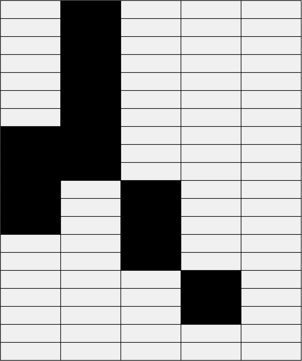
In our simulations, we generate incomplete matrices $X(\mathbf{m})$ of various sizes with values missing at randomly selected locations $\mathbf{m}$. Figure 2 illustrates an example of such matrices. In the figure, cells marked in darker shade indicate locations of missing values, and those marked in lighter shade denote known entries of the matrix. We evaluate the performance of our Algorithm 1, and compare with the above sequential methodologies on 6 example scenarios. First example E1 generates $X\in\mathbb{R}^{20\times 4}$ with $12.5\%$ entries missing from randomly selected locations, and each known data point in the range of $[-1,2]$. The task is to simultaneously impute for these missing values and select 11 rows (experiments) from $X$. In the second example E2, we create an input data matrix of same size, i.e $X\in\mathbb{R}^{20\times 4}$, but with values in range of $[0,4]$ and $10\%$ data missing at random places. The objective here in addition to imputing missing data is to select 12 experiments from the set. Similar examples, E3-E6, are generated to simulate various instances of missing data. See Table I for details.

Figure 3 illustrates the comparison of the Algorithm 1 with the above stated benchmark sequential methodologies. In particular, it plots the ratio of the A-optimal cost incurred using Algorithm 1 with the cost incurred when using the sequential methodologies for each of the experiments E1-E6 described in Table I. Note that the Algorithm 1 consistently performs better than the benchmark methods. For instance, in the example E1 our Algorithm 1 results into a solution that (a) incurs only $0.6$ times the cost incurred when using mean imputations for missing data followed by our MEP-based algorithm (assuming complete known matrix $X\in\mathbb{R}^{n\times p}$), (b) incurs only $0.52$ times the cost incurred with mean data imputation followed by the standard Fedorovs algorithm, and (c) incurs only $0.35$ times the cost incurred with mean data imputation followed by uniform sampling of experiments. Similarly, in the example E4 our Algorithm 1 (a) incurs a cost that is $0.47$ times the cost incurred by mean data imputation followed by our MEP-based algorithm (assuming complete known matrix $X$) to select experiments, (b) incurs a cost that is $0.42$ times the cost incurred when using Fedorovs algorithm for selecting experiments after mean data imputations, and (c) incurs a cost that is $0.2$ times the cost incurred when using uniform sampling for selecting experiments after mean data imputations. Further as seen from Figure 3, given a complete matrix $X$ with imputed values, MEP based Algorithm 1 consistently performs better than other standard methods like Fedorov’s exchange. Please refer to Figure 3 for details on all the other experiments.

To illustrate the benefit of annealing as done in our proposed Algorithm 1, we benchmark our results to that of direct optimization of the posed objective given by (3) using standard constrained optimization routine interior points method[47]. On first example, E1, we obtain a cost $0.57$ times lower using Algorithm 1 compared to that of of direct optimization. This demonstrates the benefit of annealing in avoiding poor local minimum. An interesting observation while performing the direct optimization using interior points method is that selection of experiments do not change much from the initialization but still, it gives a competitive cost to other algorithms. This is attributed to the imputed missing feature data in a coupled manner and hence strengthens the utility of our proposed problem (3).

Here we highlight some of the features and extensions of our proposed framework.

References

- [1] B. Durakovic and H. Basic, “Continuous quality improvement in textile processing by statistical process control tools: A case study of medium-sized company,” Periodicals of Engineering and Natural Sciences, vol. 1, no. 1, 2013.
- [2] P. Yu, M. Y. Low, and W. Zhou, “Design of experiments and regression modelling in food flavour and sensory analysis: A review,” Trends in Food Science & Technology, vol. 71, pp. 202–215, 2018.
- [3] A. Schlueter and P. Geyer, “Linking bim and design of experiments to balance architectural and technical design factors for energy performance,” Automation in Construction, vol. 86, pp. 33–43, 2018.
- [4] F. Paulo and L. Santos, “Design of experiments for microencapsulation applications: A review,” Materials Science and Engineering: C, vol. 77, pp. 1327–1340, 2017.
- [5] F. Pukelsheim, Optimal design of experiments. SIAM, 2006.
- [6] B. Settles, “Active learning,” Synthesis lectures on artificial intelligence and machine learning, vol. 6, no. 1, pp. 1–114, 2012.
- [7] Y. Deshpande and A. Montanari, “Linear bandits in high dimension and recommendation systems,” in 2012 50th Annual Allerton Conference on Communication, Control, and Computing (Allerton). IEEE, 2012, pp. 1750–1754.
- [8] A. Kulesza and B. Taskar, “Determinantal point processes for machine learning,” arXiv preprint arXiv:1207.6083, 2012.
- [9] D. C. Montgomery, E. A. Peck, and G. G. Vining, Introduction to linear regression analysis. John Wiley & Sons, 2021.
- [10] S. Jiao, Y. Gao, J. Feng, T. Lei, and X. Yuan, “Does deep learning always outperform simple linear regression in optical imaging?” Optics express, vol. 28, no. 3, pp. 3717–3731, 2020.
- [11] M. Lu, J. Zhou, C. Naylor, B. D. Kirkpatrick, R. Haque, W. A. Petri, and J. Z. Ma, “Application of penalized linear regression methods to the selection of environmental enteropathy biomarkers,” Biomarker research, vol. 5, no. 1, pp. 1–10, 2017.
- [12] J. J. Rissanen, “Fisher information and stochastic complexity,” IEEE transactions on information theory, vol. 42, no. 1, pp. 40–47, 1996.
- [13] A. Civril and M. Magdon-Ismail, “On selecting a maximum volume sub-matrix of a matrix and related problems,” Theoretical Computer Science, vol. 410, no. 47-49, pp. 4801–4811, 2009.
- [14] J. Yick, B. Mukherjee, and D. Ghosal, “Wireless sensor network survey,” Computer networks, vol. 52, no. 12, pp. 2292–2330, 2008.
- [15] C.-H. Lo and N. Ansari, “The progressive smart grid system from both power and communications aspects,” IEEE Communications Surveys & Tutorials, vol. 14, no. 3, pp. 799–821, 2011.
- [16] A. K. Fletcher, S. Rangan, and V. K. Goyal, “Estimation from lossy sensor data: Jump linear modeling and kalman filtering,” in Proceedings of the 3rd international symposium on Information processing in sensor networks, 2004, pp. 251–258.
- [17] T. E. Raghunathan, “What do we do with missing data? some options for analysis of incomplete data,” Annu. Rev. Public Health, vol. 25, pp. 99–117, 2004.
- [18] J. D. Kromrey and C. V. Hines, “Nonrandomly missing data in multiple regression: An empirical comparison of common missing-data treatments,” Educational and Psychological Measurement, vol. 54, no. 3, pp. 573–593, 1994.
- [19] O. F. Ayilara, L. Zhang, T. T. Sajobi, R. Sawatzky, E. Bohm, and L. M. Lix, “Impact of missing data on bias and precision when estimating change in patient-reported outcomes from a clinical registry,” Health and quality of life outcomes, vol. 17, no. 1, pp. 1–9, 2019.
- [20] B. Marlin, “Missing data problems in machine learning,” Ph.D. dissertation, 2008.
- [21] M. Saleh and R. Pan, “Constructing efficient experimental designs for generalized linear models,” Communications in Statistics - Simulation and Computation, vol. 45, no. 8, pp. 2827–2845, 2016. [Online]. Available: https://doi.org/10.1080/03610918.2014.927486
- [22] A. Heredia-Langner, W. M. Carlyle, D. C. Montgomery, C. M. Borror, and G. C. Runger, “Genetic algorithms for the construction of d-optimal designs,” Journal of quality technology, vol. 35, no. 1, pp. 28–46, 2003.
- [23] A. J. Miller and N.-K. Nguyen, “Algorithm as 295: A fedorov exchange algorithm for d-optimal design,” Journal of the royal statistical society. series c (applied statistics), vol. 43, no. 4, pp. 669–677, 1994.
- [24] Z. Allen-Zhu, Y. Li, A. Singh, and Y. Wang, “Near-optimal design of experiments via regret minimization,” in Proceedings of the 34th International Conference on Machine Learning, ser. Proceedings of Machine Learning Research, D. Precup and Y. W. Teh, Eds., vol. 70. International Convention Centre, Sydney, Australia: PMLR, 06–11 Aug 2017, pp. 126–135. [Online]. Available: http://proceedings.mlr.press/v70/allen-zhu17e.html
- [25] S. N. Ravi, V. Ithapu, S. Johnson, and V. Singh, “Experimental design on a budget for sparse linear models and applications,” in Proceedings of The 33rd International Conference on Machine Learning, ser. Proceedings of Machine Learning Research, M. F. Balcan and K. Q. Weinberger, Eds., vol. 48. New York, New York, USA: PMLR, 20–22 Jun 2016, pp. 583–592. [Online]. Available: http://proceedings.mlr.press/v48/ravi16.html
- [26] A. Deshpande and L. Rademacher, “Efficient volume sampling for row/column subset selection,” in 2010 IEEE 51st Annual Symposium on Foundations of Computer Science, 2010, pp. 329–338.
- [27] C. Li, S. Jegelka, and S. Sra, “Polynomial time algorithms for dual volume sampling,” 2017.
- [28] H. Avron and C. Boutsidis, “Faster subset selection for matrices and applications,” SIAM Journal on Matrix Analysis and Applications, vol. 34, no. 4, pp. 1464–1499, 2013.
- [29] Y. Wang, A. W. Yu, and A. Singh, “On computationally tractable selection of experiments in measurement-constrained regression models,” Journal of Machine Learning Research, vol. 18, no. 143, pp. 1–41, 2017. [Online]. Available: http://jmlr.org/papers/v18/17-175.html
- [30] A. Nikolov, M. Singh, and U. T. Tantipongpipat, “Proportional volume sampling and approximation algorithms for a-optimal design,” in Proceedings of the Thirtieth Annual ACM-SIAM Symposium on Discrete Algorithms. SIAM, 2019, pp. 1369–1386.
- [31] M. Dereziński, M. K. Warmuth, and D. Hsu, “Leveraged volume sampling for linear regression,” arXiv preprint arXiv:1802.06749, 2018.
- [32] I. Eekhout, H. C. de Vet, J. W. Twisk, J. P. Brand, M. R. de Boer, and M. W. Heymans, “Missing data in a multi-item instrument were best handled by multiple imputation at the item score level,” Journal of clinical epidemiology, vol. 67, no. 3, pp. 335–342, 2014.
- [33] Z. Zhang, “Missing data imputation: focusing on single imputation,” Annals of translational medicine, vol. 4, no. 1, 2016.
- [34] N. K. Malhotra, “Analyzing marketing research data with incomplete information on the dependent variable,” Journal of Marketing Research, vol. 24, no. 1, pp. 74–84, 1987.
- [35] A. Dempster, N. Laird, and D. Rubin, “Maximal likelihood form incomplete data via the em algorithm,” J. Roy. Statist. Soc, pp. 1–38.
- [36] N.-K. Nguyen and A. J. Miller, “A review of some exchange algorithms for constructing discrete d-optimal designs,” Computational Statistics & Data Analysis, vol. 14, no. 4, pp. 489–498, 1992.
- [37] E. T. Jaynes, “Information theory and statistical mechanics,” Physical review, vol. 106, no. 4, p. 620, 1957.
- [38] K. Rose, “Deterministic annealing for clustering, compression, classification, regression, and related optimization problems,” Proceedings of the IEEE, vol. 86, no. 11, pp. 2210–2239, 1998.
- [39] A. Dubey, O. Gupta, R. Raskar, and N. Naik, “Maximum-entropy fine-grained classification,” arXiv preprint arXiv:1809.05934, 2018.
- [40] P. V. Gehler and O. Chapelle, “Deterministic annealing for multiple-instance learning,” in Artificial Intelligence and Statistics. PMLR, 2007, pp. 123–130.
- [41] A. Rao, K. Rose, and A. Gersho, “Design of robust hmm speech recognizers using deterministic annealing,” in 1997 IEEE Workshop on Automatic Speech Recognition and Understanding Proceedings. IEEE, 1997, pp. 466–473.
- [42] A. Srivastava and S. M. Salapaka, “Simultaneous facility location and path optimization in static and dynamic networks,” IEEE Transactions on Control of Network Systems, vol. 7, no. 4, pp. 1700–1711, 2020.
- [43] S. F. Gull and J. Skilling, “Maximum entropy method in image processing,” in IEE Proceedings F (Communications, Radar and Signal Processing), vol. 131, no. 6. IET, 1984, pp. 646–659.
- [44] M. Baranwal, A. Srivastava, and S. M. Salapaka, “Multiway k-cut in static and dynamic graphs: A maximum entropy principle approach,” in 2019 IEEE 58th Conference on Decision and Control (CDC). IEEE, 2019, pp. 3948–3953.
- [45] A. Banerjee, I. Dhillon, J. Ghosh, S. Merugu, and D. S. Modha, “A generalized maximum entropy approach to bregman co-clustering and matrix approximation,” The Journal of Machine Learning Research, vol. 8, pp. 1919–1986, 2007.
- [46] Y. Xu, S. M. Salapaka, and C. L. Beck, “Aggregation of graph models and markov chains by deterministic annealing,” IEEE Transactions on Automatic Control, vol. 59, no. 10, pp. 2807–2812, 2014.
- [47] R. H. Byrd, M. E. Hribar, and J. Nocedal, “An interior point algorithm for large-scale nonlinear programming,” SIAM Journal on Optimization, vol. 9, no. 4, pp. 877–900, 1999.