In this section, we review two-dimensional bosonic oriented TQFTs with fusion category symmetry $\mathcal{C}$. We will enumerate the consistency conditions on transition amplitudes by following [11]. We first assign a vector space $V_{x}$ to a circle with a topological defect $x$. When a topological defect is a direct sum $x\oplus y$, the vector space $V_{x\oplus y}$ is given by the direct sum of two vector spaces $V_{x}$ and $V_{y}$. To define the vector space on a circle with multiple topological defects, we need to specify the base point on the circle. Once we fix the base point, the vector space on a circle with topological defects $x,y,z,\cdots$ is defined as the vector space on a circle with a single topological defect labeled by the tensor product $((x\otimes y)\otimes z)\otimes\cdots$, see figure 2.

The vector space on a disjoint union of circles is given by the tensor product of the vector spaces on each circle.

Next, we consider transition amplitudes between the vector spaces. Let us begin with the transition amplitude for a cylinder. There are two types of cylinder amplitudes as shown in figure 3: one is the transition amplitude corresponding to a topological point operator $f\in\mathop{\mathrm{Hom}}(x,x^{\prime})$, and the other is the transition amplitude corresponding to a change of the base point.

The former is denoted by $Z(f):V_{x}\rightarrow V_{x^{\prime}}$. In particular, the identity morphism $\mathrm{id}_{x}$ corresponds to the identity map $\mathrm{id}_{V_{x}}$. The latter is denoted by $X_{xy}:V_{x\otimes y}\rightarrow V_{y\otimes x}$ when the base point on a circle with two topological defects $x$ and $y$ is moved from the left of $x$ to the right of $x$. We call the trajectory of the base point the auxiliary line.

To make the cylinder amplitude well-defined, we require that the composition of morphisms $f$ and $g$ gives rise to the composition of the transition amplitudes $Z(f)$ and $Z(g)$, see figure 4:

$$Z(g\circ f)=Z(g)\circ Z(f).$$

(O1)

This makes $Z$ a functor from $\mathcal{C}$ to $\mathrm{Vec}$ where $Z(x)$ is defined as the vector space $V_{x}$ for every object $x$ of $\mathcal{C}$.

We demand that this functor is $\mathbb{C}$-linear in morphisms because a linear combination of topological point operators $f,f^{\prime}\in\mathop{\mathrm{Hom}}(x,x^{\prime})$ results in a linear combination of transition amplitudes, see figure 5:

$$Z(\alpha f+\alpha^{\prime}f^{\prime})=\alpha Z(f)+\alpha^{\prime}Z(f^{\prime}),\quad\forall\alpha,\alpha^{\prime}\in\mathbb{C}.$$

(O2)

Furthermore, we require that the transition amplitudes do not depend on the shape of the auxiliary line if we fix the base points on the initial and final circles. In particular, the transition amplitudes are invariant under winding the auxiliary line around a cylinder, see figure 6.

This implies that the linear map $X_{xy}:V_{x\otimes y}\rightarrow V_{y\otimes x}$ is an isomorphism, whose inverse is given by $X_{yx}$:

$$X_{xy}=X_{yx}^{-1}.$$

(O3)

We also require that a change of the base point commutes with morphisms $f\in\mathop{\mathrm{Hom}}(x,x^{\prime})$ and $g\in\mathop{\mathrm{Hom}}(y,y^{\prime})$ as shown in figure 7:

	$\displaystyle Z(\mathrm{id}_{y}\otimes f)\circ X_{xy}$	$\displaystyle=X_{x^{\prime}y}\circ Z(f\otimes\mathrm{id}_{y}),$		(O4)
	$\displaystyle Z(g\otimes\mathrm{id}_{x})\circ X_{xy}$	$\displaystyle=X_{xy^{\prime}}\circ Z(\mathrm{id}_{x}\otimes g).$

These equations indicate that the auxiliary line is transparent to topological point operators.

The last constraint on the cylinder amplitude is that moving a base point across the topological defects $x$ and $y$ at the same time is equivalent to moving a base point across $x$ and $y$ successively. This leads to the following consistency condition:

$$X_{y,z\otimes x}\circ Z(\alpha_{yzx})\circ X_{x,y\otimes z}\circ Z(\alpha_{xyz})=Z(\alpha_{zxy}^{-1})\circ X_{x\otimes y,z}.$$

(O5)

In particular, if we choose $x=y=1$, we obtain $X_{1,x}=\mathrm{id}_{V_{x}}$, which means that moving the base point across a trivial defect does not affect the transition amplitude.⁴⁴ 4 We recall that the left and right units are chosen to be the identity morphism. This completes the consistency conditions on the cylinder amplitude.

For later convenience, we define the generalized associator $\mathcal{A}_{p\rightarrow p^{\prime}}:V_{p}\rightarrow V_{p^{\prime}}$ as a composition of isomorphisms $X$ and $Z(\alpha)$, where $p$ is a tensor product of any number of objects and $p^{\prime}$ is a cyclic permutation of $p$ with arbitrary parentheses. For example, the generalized associator $\mathcal{A}_{(x\otimes y)\otimes z\rightarrow(z\otimes x)\otimes y}$ is given by both sides of eq. (O5). In general, there are many ways to construct an isomorphism from $V_{p}$ to $V_{p^{\prime}}$ only from $X$ and $Z(\alpha)$. However, they give rise to the same isomorphism due to eq. (O5). This means that the generalized associator $\mathcal{A}_{p\rightarrow p^{\prime}}$ is unique, although it has many distinct-looking expressions.

The transition amplitude for a general surface can be constructed from the cylinder amplitude and the following four basic elements: the unit $i:\mathbb{C}\rightarrow V_{1}$, the counit $\epsilon:V_{1}\rightarrow\mathbb{C}$, the multiplication $M_{xy}:V_{x}\otimes V_{y}\rightarrow V_{x\otimes y}$, and the comultiplication $\Delta_{xy}:V_{x\otimes y}\rightarrow V_{x}\otimes V_{y}$, see also figure 8 for diagrammatic representations.

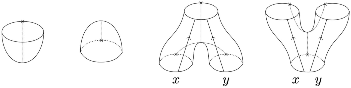
For unitary quantum field theories, the counit $\epsilon$ and the comultiplication $\Delta_{xy}$ are the adjoints of the unit $i$ and the multiplication $M_{xy}$ respectively (with respect to the non-degenerate pairing (O6)):

$$\epsilon=i^{\dagger},\quad\Delta_{xy}=M_{xy}^{\dagger}.$$

(3.1)

More generally, a transition amplitude changes to its adjoint when the corresponding surface is turned upside down, or equivalently when the time direction is reversed.

Any two-dimensional surface $\Sigma$ can be obtained by successively gluing cylinders and the basic elements shown in figure 8. The transition amplitude for a surface $\Sigma$ is defined as the composition of the linear maps corresponding to cylinders and the basic elements that appear in the decomposition of $\Sigma$. However, the way to decompose $\Sigma$ is not unique in general. Therefore, we need to impose consistency conditions so that the transition amplitudes do not depend on a decomposition. Such consistency conditions can be listed as follows [11]:

Non-degenerate pairing

(figure 9)

$$\text{The pairing }\epsilon\circ Z(\mathrm{ev}_{x}^{L})\circ M_{x^{*},x}:V_{x^{*}}\otimes V_{x}\rightarrow\mathbb{C}\text{ is non-degenerate}.$$

(O6)

This non-degenerate pairing is related to the inner product of the Hilbert space via $CPT$ conjugation [7, 38].

Unit constraint

(figure 10)

The unit $i$ acts as the unit of the multiplication $M$:

$$M_{1x}(i(1)\otimes v_{x})=M_{x1}(v_{x}\otimes i(1))=v_{x},\quad\forall v_{x}\in V_{x}.$$

(O7)

Associativity

(figure 11)

The multiplication $M$ is associative up to associator:

$$Z(\alpha_{xyz})\circ M_{x\otimes y,z}\circ(M_{xy}\otimes\mathrm{id}_{V_{z}})=M_{x,y\otimes z}\circ(\mathrm{id}_{V_{x}}\otimes M_{yz})\circ\alpha_{V_{x}V_{y}V_{z}}^{\mathrm{Vec}},$$

(O8)

where $\alpha_{V_{x}V_{y}V_{z}}^{\mathrm{Vec}}$ is the associator of the category of vector spaces $\mathrm{Vec}$, which is chosen to be the identity map $\alpha_{V_{x}V_{y}V_{z}}^{\mathrm{Vec}}=\mathrm{id}_{V_{x}\otimes V_{y}\otimes V_{z}}$ by identifying $(V_{x}\otimes V_{y})\otimes V_{z}$ with $V_{x}\otimes(V_{y}\otimes V_{z})$.

Twisted commutativity

(figure 12)

The multiplication $M$ is commutative up to the change of the base point:

$$M_{yx}\circ c_{V_{x}V_{y}}=X_{xy}\circ M_{xy},$$

(O9)

where $c_{V_{x}V_{y}}:V_{x}\otimes V_{y}\rightarrow V_{y}\otimes V_{x}$ is the symmetric braiding of $\mathrm{Vec}$, which is defined by $c_{V_{x}V_{y}}(v_{x}\otimes v_{y}):=v_{y}\otimes v_{x}$ for any $v_{x}\in V_{x}$ and $v_{y}\in V_{y}$.

Commutativity of topological point operators and the multiplication

(figure 13)

Topological point operators commute with the multiplication $M$:

	$\displaystyle M_{x^{\prime}y}\circ(Z(f)\otimes\mathrm{id}_{V_{y}})$	$\displaystyle=Z(f\otimes\mathrm{id}_{y})\circ M_{xy},\quad\forall f\in\mathop{\mathrm{Hom}}(x,x^{\prime}),$		(O10)
	$\displaystyle M_{xy^{\prime}}\circ(\mathrm{id}_{V_{x}}\otimes Z(g))$	$\displaystyle=Z(\mathrm{id}_{x}\otimes g)\circ M_{xy},\quad\forall g\in\mathop{\mathrm{Hom}}(y,y^{\prime}).$

The uniqueness of the multiplication

(figure 14)

The multiplication $M$ uniquely determines a map for topologically equivalent configurations of topological defects on the pants diagram:

		$\displaystyle Z((\mathrm{id}_{x}\otimes\mathrm{ev}_{z}^{L})\otimes\mathrm{id}_{y^{*}})\circ\mathcal{A}_{(x\otimes z^{*})\otimes(z\otimes y^{*})\rightarrow(x\otimes(z^{*}\otimes z))\otimes y^{*}}\circ M_{x\otimes z^{*},z\otimes y^{*}}$		(O11)
	$\displaystyle=$	$\displaystyle Z(\mathrm{id}_{x\otimes y^{*}}\otimes\mathrm{ev}_{z}^{R})\circ\mathcal{A}_{(z^{*}\otimes x)\otimes(y^{*}\otimes z)\rightarrow(x\otimes y^{*})\otimes(z\otimes z^{*})}\circ M_{z^{*}\otimes x,y^{*}\otimes z}\circ(X_{x,z^{*}}\otimes X_{z,y^{*}}).$

Consistency on the torus

(figure 15)

Different ways to decompose a twice-punctured torus give the same transition amplitude:

		$\displaystyle\mathcal{A}_{(y\otimes x)\otimes(w\otimes z)\rightarrow(x\otimes w)\otimes(z\otimes y)}\circ M_{y\otimes x,w\otimes z}\circ(X_{xy}\otimes X_{zw})\circ\Delta_{x\otimes y,z\otimes w}$		(O12)
	$\displaystyle=$	$\displaystyle M_{x\otimes w,z\otimes y}\circ(X_{wx}\otimes X_{yz})\circ\Delta_{w\otimes x,y\otimes z}\circ\mathcal{A}_{(x\otimes y)\otimes(z\otimes w)\rightarrow(w\otimes x)\otimes(y\otimes z)}.$

In summary, a two-dimensional bosonic oriented TQFT with fusion category symmetry is given by a quadruple $(Z,X,M,i)$ that satisfies the consistency conditions (O1)–(O12).⁵⁵ 5 In [11], there is an additional consistency condition called the cyclic symmetry of the multiplication. However, this condition turns out to be satisfied as a consequence of (O6) and (O8).

In this section, we classify bosonic SPT phases with fusion category symmetry $\mathcal{C}$ by solving the consistency conditions (O1)–(O12). To focus on the solutions that describe SPT phases, we further impose the condition that the ground state is unique on a circle without topological defects, i.e. $\mathop{\mathrm{dim}}V_{1}=1$. More generally, the dimension of the vector space $V_{x}$ for an SPT phase is equal to the quantum dimension of the object $x$

$$\mathop{\mathrm{dim}}V_{x}=\mathop{\mathrm{dim}}x,$$

(3.2)

which can be seen from modular invariance of the partition function on a torus [12].

For SPT phases, the unit $i:\mathbb{C}\rightarrow V_{1}$ is an isomorphism because it is a non-zero linear map between one-dimensional vector spaces. In particular, $i$ is unitary if the partition function on a sphere is unity:

$$i^{\dagger}\circ i=1.$$

(3.3)

In the following, we assume that this condition is satisfied. Furthermore, we assume that the multiplication $M_{xy}:V_{x}\otimes V_{y}\rightarrow V_{x\otimes y}$ is also unitary:

$$M_{xy}^{\dagger}=M_{xy}^{-1}\Leftrightarrow\hbox{$\vbox{\hbox{\resizebox{}{}{{\hbox{{}}}}}}$}~=~\hbox{$\vbox{\hbox{\resizebox{}{}{{\hbox{{}}}}}}$}.$$

(3.4)

This equation reduces to eq. (3.2) if we form a loop of $x$ by choosing $y=x^{*}$ and close the punctures with a cap and its adjoint.

Now, we solve the consistency conditions (O1)–(O12) under the constraints (3.3) and (3.4). We first notice that $Z:\mathcal{C}\rightarrow\mathrm{Vec}$ is a functor by (O1), where an object $x$ is mapped to a vector space $V_{x}$ and a morphism $f\in\mathop{\mathrm{Hom}}(x,y)$ is mapped to a linear map $Z(f):V_{x}\rightarrow V_{y}$. We recall that the functor $Z$ is additive in objects in the sense that the direct sum of objects $x$ and $y$ is mapped to the direct sum of vector spaces $V_{x}$ and $V_{y}$. This functor is also $\mathbb{C}$-linear in morphisms due to (O2). Furthermore, (O7) and (O8) indicate that the triple $(Z,M,i)$ is a monoidal functor where the naturality of the isomorphism $M_{xy}$ follows from (O10). Thus, $(Z,M,i)$ is a tensor functor from $\mathcal{C}$ to $\mathrm{Vec}$, namely a fiber functor. In this way, we can extract the data of a fiber functor from an SPT phase with fusion category symmetry. Conversely, we can show that the data of a fiber functor $(Z,M,i)$ is sufficient to construct a solution of (O1)–(O12) as we will see below. In other words, the other consistency conditions are automatically satisfied when $(Z,M,i)$ is a fiber functor.

Since $M_{xy}$ is unitary (3.4), the isomorphism $X_{xy}$ is determined by (O9) as

$$X_{xy}=M_{yx}\circ c_{V_{x}V_{y}}\circ M_{xy}^{-1}.$$

(3.5)

This satisfies (O3) because $c_{V_{x}V_{y}}$ is the symmetric braiding of $\mathrm{Vec}$. Furthermore, the naturality of $M_{xy}$ and $c_{V_{x}V_{y}}$ implies that $X_{xy}$ is also natural (O4). The non-degeneracy of the pairing (O6) is guaranteed by the equality

$$\hbox{$\vbox{\hbox{\resizebox{}{}{{\hbox{{}}}}}}$}~=~\hbox{$\vbox{\hbox{\resizebox{}{}{{\hbox{{}}}}}}$},$$

(3.6)

which follows from the Frobenius relation represented by the following commutative diagram:

(3.7)

To proceed further, we notice that a linear map from $V_{x_{1}\otimes y_{1}\otimes\cdots}\otimes V_{x_{2}\otimes y_{2}\otimes\cdots}\otimes\cdots$ to $V_{x^{\prime}_{1}\otimes y^{\prime}_{1}\otimes\cdots}\otimes V_{x^{\prime}_{2}\otimes y^{\prime}_{2}\otimes\cdots}\otimes\cdots$ that consists only of $M$ and $c$ is uniquely determined by the permutation of the topological defect $(x_{1},y_{1},\cdots,x_{2},y_{2},\cdots)\rightarrow(x^{\prime}_{1},y^{\prime}_{1},\cdots,x^{\prime}_{2},y^{\prime}_{2},\cdots)$ and the change of the parentheses. The same holds for a linear map that consists only of $M$, $c$, $Z(\alpha)$, and $X$ because $Z(\alpha)$ and $X$ can be expressed in terms of $M$ and $c$ due to (O8) and (O9). This shows (O5) and (O12). This also reduces the consistency condition (O11) to the following commutative diagram:

(3.8)

The commutativity of the left square in the above diagram defines the evaluation morphism $\mathrm{ev}_{V_{z}}^{L}:V_{z^{*}}\otimes V_{z}\rightarrow\mathbb{C}$, which is the non-degenerate pairing (O6). Accordingly, we can consider $V_{z^{*}}$ as the dual vector space of $V_{z}$. If we denote a basis of $V_{z}$ as $\{e_{i}\mid i=1,2,\cdots,\mathop{\mathrm{dim}}V_{z}\}$, the dual basis $\{e^{i}\mid i=1,2,\cdots,\mathop{\mathrm{dim}}V_{z^{*}}=\mathop{\mathrm{dim}}V_{z}\}$ of $V_{z^{*}}$ is defined by

$$\mathrm{ev}_{V_{z}}^{L}(e^{i}\otimes e_{j})=\delta^{i}_{j},$$

(3.9)

where $\delta^{i}_{j}$ is the Kronecker delta. Equation (2.5) implies that the coevaluation morphism $\mathrm{coev}_{V_{z}}^{L}:\mathbb{C}\rightarrow V_{z}\otimes V_{z^{*}}$ is given by the embedding

$$\mathrm{coev}_{V_{z}}^{L}(1)=\sum_{i=1}^{\mathop{\mathrm{dim}}V_{z}}e_{i}\otimes e^{i},$$

(3.10)

whose adjoint agrees with the right evaluation morphism $\mathrm{ev}_{V_{z}}^{R}$ defined by the commutativity of the right square in the diagram (3.8):

$$\mathrm{ev}_{V_{z}}^{R}(e_{i}\otimes e^{j})=\delta_{i}^{j}.$$

(3.11)

From eqs. (3.9) and (3.11), we find that the bottom triangle in (3.8) is commutative.

In summary, the solutions of the consistency conditions (O1)–(O12) for fusion category SPT phases are in one-to-one correspondence with fiber functors of the fusion category $\mathcal{C}$. To classify fusion category SPT phases, we regard naturally isomorphic fiber functors as the same SPT phase because a natural isomorphism between fiber functors corresponds to a change of the bases of the vector spaces. Therefore, bosonic SPT phases with fusion category symmetry $\mathcal{C}$ are classified by isomorphism classes of fiber functors of $\mathcal{C}$.

A two-dimensional unoriented TQFT with finite group symmetry is formulated in [7, 9] as a set of consistency conditions on algebraic data.⁶⁶ 6 A two-dimensional unoriented TQFT without internal symmetry is formulated in [39]. Quantum field theories on unoriented manifolds are of interest in recent studies on topological phases of matter [40, 41, 42, 43, 44, 45, 46, 47, 48, 49, 50, 51, 52, 53, 54]. In this section, we reformulate 2d unoriented TQFTs to incorporate fusion category symmetries. We assume that the total symmetry splits into time-reversal symmetry and finite internal symmetry. In this case, we can treat orientation-reversing defects and symmetry defects separately.

The algebraic data of an unoriented TQFT consist of the following linear maps in addition to the algebraic data of an oriented TQFT: the orientation-reversing isomorphism $\phi_{x}:V_{x}\rightarrow V_{x^{*}}$ and the cross-cap amplitude $\theta_{x,y}:V_{x\otimes y}\rightarrow V_{x^{*}\otimes y}$, see also figure 16.

In particular, $\phi$ represents the linear action of $CP$ symmetry, which we assume to be unitary, rather than the anti-linear action of time-reversal symmetry. We can avoid anti-linear maps by using $CPT$ symmetry [7]. A variant of the cross-cap amplitude as shown in figure 17 can be computed by composing the cross-cap amplitude $\theta$ and the generalized associators $\mathcal{A}$.

A general unoriented surface can be decomposed into the following building blocks and their adjoints: a cylinder, a cap, a pair of pants, and a cylinder with a cross-cap. Correspondingly, the transition amplitude for a general unoriented surface is given by the composition of the transition amplitudes for these elements that appear in the decomposition. However, the decomposition is not unique in general. Therefore, we need to impose consistency conditions so that the transition amplitude does not depend on a decomposition. In the following, we list the consistency conditions that involve $\phi$ and $\theta$.

Invariance of the unit

The unit $i:\mathbb{C}\rightarrow V_{1}$ is invariant under the action of the orientation-reversing isomorphism

$$\hbox{$\vbox{\hbox{\resizebox{}{}{{\hbox{{}}}}}}$}~=~\hbox{$\vbox{\hbox{\resizebox{}{}{{\hbox{{}}}}}}$}.$$

(U1)

Involution

The orientation-reversing isomorphism is involutive up to pivotal structure $a_{x}:x\rightarrow x^{**}$

$$\hbox{$\vbox{\hbox{\resizebox{}{}{{\hbox{{}}}}}}$}~=~\hbox{$\vbox{\hbox{\resizebox{}{}{{\hbox{{}}}}}}$}.$$

(U2)

Commutativity of the orientation reversal and the change of the base point

The orientation-reversing isomorphism commutes with the change of the base point:

$$\hbox{$\vbox{\hbox{\resizebox{}{}{{\hbox{{}}}}}}$}~=~\hbox{$\vbox{\hbox{\resizebox{}{}{{\hbox{{}}}}}}$}.$$

(U3)

Orientation reversal of a topological point operator

The orientation-reversing symmetry acts on a topological point operator $f\in\mathop{\mathrm{Hom}}(x,y)$ and turn it into another topological point operator $\overline{f}\in\mathop{\mathrm{Hom}}(x^{*},y^{*})$ such that

$$\hbox{$\vbox{\hbox{\resizebox{}{}{{\hbox{{}}}}}}$}~=~\hbox{$\vbox{\hbox{\resizebox{}{}{{\hbox{{}}}}}}$},\quad\hbox{$\vbox{\hbox{\resizebox{}{}{{\hbox{{}}}}}}$}~=~\hbox{$\vbox{\hbox{\resizebox{}{}{{\hbox{{}}}}}}$}.$$

(U4)

Cross-cap on a folded topological defect

We can move the position of a cross-cap along a folded topological defect line:

$$\hbox{$\vbox{\hbox{\resizebox{}{}{{\hbox{{}}}}}}$}~=~\hbox{$\vbox{\hbox{\resizebox{}{}{{\hbox{{}}}}}}$}.$$

(U5)

Deformation of a topological defect through a cross-cap

A topological defect that passes a cross-cap twice can avoid the cross-cap by a deformation:

$$\hbox{$\vbox{\hbox{\resizebox{}{}{{\hbox{{}}}}}}$}~=~\hbox{$\vbox{\hbox{\resizebox{}{}{{\hbox{{}}}}}}$},\quad\quad\hbox{$\vbox{\hbox{\resizebox{}{}{{\hbox{{}}}}}}$}~=~\hbox{$\vbox{\hbox{\resizebox{}{}{{\hbox{{}}}}}}$}.$$

(U6)

We also have similar equations for the diagrams flipped horizontally.

Commutativity of the cross-cap and the orientation reversal

The orientation-reversing isomorphism commutes with the cross-cap amplitude:

$$\hbox{$\vbox{\hbox{\resizebox{}{}{{\hbox{{}}}}}}$}~=~\hbox{$\vbox{\hbox{\resizebox{}{}{{\hbox{{}}}}}}$}.$$

(U7)

Möbius identity

Two different ways to compute the transition amplitude for the punctured Möbius strip lead to the same result:

$$\hbox{$\vbox{\hbox{\resizebox{}{}{{\hbox{{}}}}}}$}~=~\hbox{$\vbox{\hbox{\resizebox{}{}{{\hbox{{}}}}}}$}.$$

(U8)

Equivariance of the multiplication

The multiplication is equivariant with respect to the orientation-reversing isomorphism:

$$\hbox{$\vbox{\hbox{\resizebox{}{}{{\hbox{{}}}}}}$}~=~\hbox{$\vbox{\hbox{\resizebox{}{}{{\hbox{{}}}}}}$}.$$

(U9)

Compatibility of the cross-cap amplitude and the multiplication

We can move the position of a cross-cap through the pants diagram:

$$\hbox{$\vbox{\hbox{\resizebox{}{}{{\hbox{{}}}}}}$}~=~\hbox{$\vbox{\hbox{\resizebox{}{}{{\hbox{{}}}}}}$},\quad\hbox{$\vbox{\hbox{\resizebox{}{}{{\hbox{{}}}}}}$}~=~\hbox{$\vbox{\hbox{\resizebox{}{}{{\hbox{{}}}}}}$}.$$

(U10)

Klein identity

Two different decompositions of the twice-punctured Klein bottle give rise to the same transition amplitude:

$$\hbox{$\vbox{\hbox{\resizebox{}{}{{\hbox{{}}}}}}$}~=~\hbox{$\vbox{\hbox{\resizebox{}{}{{\hbox{{}}}}}}$}.$$

(U11)

We need to check the consistency of the assignment of the transition amplitudes. There are three types of consistency as follows:

1. 1.

   consistency under changes of the time function,

2. 2.

   consistency under deformations of topological defects on each basic element, and

3. 3.

   consistency under the composition of the orientation-reversing isomorphism.

Let us begin with the consistency of type 1. The transition amplitudes must be invariant under changes of the time function. As discussed in the appendix of [7], we have two consistency conditions of this type for unoriented surfaces: one is the consistency on a pair of pants with a cross-cap and the other is the consistency on a twice-punctured Klein bottle. These consistency conditions are given by (U10) and (U11) respectively. Next, we consider the consistency of type 2. Topologically equivalent configurations of topological defects on a basic element give rise to the same transition amplitude. For this type of consistency conditions, it suffices to consider the consistency on a cylinder with a cross-cap because the consistency on the other basic elements is already considered in oriented TQFTs. The consistency on a cylinder with a cross-cap is given by (U5) and (U6). Finally, we have the consistency conditions of type 3 for each basic element as follows: (U2) and (U3) for a cylinder, (U1) for a cap, (U9) for a pair of pants, and (U7) and (U8) for a cylinder with a cross-cap. The remaining equation (U4) is the consistency of topological point operators. This completes the consistency conditions on transition amplitudes for unoriented surfaces. Therefore, a two-dimensional bosonic unoriented TQFT with fusion category symmetry $\mathcal{C}$ is described by a sextuple $(Z,X,M,i,\phi,\theta)$ that satisfies (O1)–(O12) and (U1)–(U11). As we will see in appendix A, this reduces to an unoriented equivariant TQFT when the symmetry is given by a finite group $\mathbb{Z}_{2}^{T}\times G$.

In this section, we classify fusion category SPT phases with time-reversal symmetry by solving the consistency conditions (U1)–(U11) under the constraints (3.3) and (3.4). We first recall that the triple $(Z,M,i):\mathcal{C}\rightarrow\mathrm{Vec}$ is a fiber functor and $X$ is given by eq. (3.5). In particular, the multiplication $M_{x,y}$ is unitary. Therefore, the cross-cap amplitude $\theta_{x,y}$ is determined by $\theta_{x,1}$ via eq. (U10) as follows:

$$\hbox{$\vbox{\hbox{\resizebox{}{}{{\hbox{{}}}}}}$}~=~\hbox{$\vbox{\hbox{\resizebox{}{}{{\hbox{{}}}}}}$}.$$

(4.1)

Conversely, the consistency condition (U10) follows from the above equation. Furthermore, the Klein identity (U11) reduces to

$$\hbox{$\vbox{\hbox{\resizebox{}{}{{\hbox{{}}}}}}$}~=~\hbox{$\vbox{\hbox{\resizebox{}{}{{\hbox{{}}}}}}$}.$$

(4.2)

This implies that the cross-cap amplitude $\theta_{x,y}$ is an isomorphism. By using eqs. (4.1) and (4.2), the equivariance (U9) can be simplified as follows:

$$\hbox{$\vbox{\hbox{\resizebox{}{}{{\hbox{{}}}}}}$}~=~\hbox{$\vbox{\hbox{\resizebox{}{}{{\hbox{{}}}}}}$}\Leftrightarrow\hbox{$\vbox{\hbox{\resizebox{}{}{{\hbox{{}}}}}}$}~=~\hbox{$\vbox{\hbox{\resizebox{}{}{{\hbox{{}}}}}}$}\Leftrightarrow\hbox{$\vbox{\hbox{\resizebox{}{}{{\hbox{{}}}}}}$}~=~\hbox{$\vbox{\hbox{\resizebox{}{}{{\hbox{{}}}}}}$}.$$

(4.3)

More generally, we obtain

$$\hbox{$\vbox{\hbox{\resizebox{}{}{{\hbox{{}}}}}}$}~=~\hbox{$\vbox{\hbox{\resizebox{}{}{{\hbox{{}}}}}}$},$$

(4.4)

from (U2). The above equations indicate that the orientation-reversing isomorphism acts trivially on the vector space $V_{1}$, which shows (U1).

As we will see below, it turns out that the remaining consistency conditions (U3)–(U8) follow from eqs. (4.1), (4.2), (4.4) and the consistency conditions of oriented TQFTs. We first notice that (U3), (U4), (U7), and (U8) immediately follow from eqs. (4.1), (4.2), and (4.4). To show the consistency condition (U5), it is convenient to compose the cross-cap amplitude to both sides:

$$\hbox{$\vbox{\hbox{\resizebox{}{}{{\hbox{{}}}}}}$}~=~\hbox{$\vbox{\hbox{\resizebox{}{}{{\hbox{{}}}}}}$}$$

(4.5)

This equation is equivalent to (U5) because the cross-cap amplitude is an isomorphism. The left-hand side can be written as

$$\mathrm{(LHS)}=\hbox{$\vbox{\hbox{\resizebox{}{}{{\hbox{{}}}}}}$}~=~\hbox{$\vbox{\hbox{\resizebox{}{}{{\hbox{{}}}}}}$},$$

(4.6)

where the second equality follows from the relation (2.4) between the left and right coevaluation morphisms. On the other hand, the right-hand side can be computed as

$$\mathrm{(RHS)}=\hbox{$\vbox{\hbox{\resizebox{}{}{{\hbox{{}}}}}}$}~=~\hbox{$\vbox{\hbox{\resizebox{}{}{{\hbox{{}}}}}}$}~=~\hbox{$\vbox{\hbox{\resizebox{}{}{{\hbox{{}}}}}}$}=\mathrm{(LHS)}.$$

(4.7)

The second equality follows from the fact that the orientation reversal of the right coevaluation morphism $\mathrm{coev}^{R}_{x}$ is given by $\overline{\mathrm{coev}^{R}_{x}}=\mathrm{coev}^{L}_{x^{*}}$, which can be seen from the unitarity of $\phi_{x}$ and the first equation of (U4). Indeed, when $\phi_{x}$ is unitary, the orientation reversal of the coevaluation morphism defined by the first equation of (U4) satisfies

$$\hbox{$\vbox{\hbox{\resizebox{}{}{{\hbox{{}}}}}}$}~=~\hbox{$\vbox{\hbox{\resizebox{}{}{{\hbox{{}}}}}}$},$$

(4.8)

which implies $\overline{\mathrm{coev}^{R}_{x}}=\mathrm{coev}^{L}_{x^{*}}$ and $\overline{\mathrm{coev}^{L}_{x}}=\mathrm{coev}^{R}_{x^{*}}$. We note that this shows the first equation of (U6). Finally, we consider the second equation of (U6). The left-hand side and the right-hand side can be written as

$$\mathrm{(LHS)}=\hbox{$\vbox{\hbox{\resizebox{}{}{{\hbox{{}}}}}}$},\quad\quad\mathrm{(RHS)}=\hbox{$\vbox{\hbox{\resizebox{}{}{{\hbox{{}}}}}}$}.$$

(4.9)

We notice that both the left-hand side and the right-hand side have the orientation-reversing isomorphism and the cross-cap amplitude in common, which can be eliminated from the equality $(\mathrm{LHS})=(\mathrm{RHS})$ because they are isomorphisms. Hence, this equation reduces to the equality of the transition amplitudes for oriented surfaces. By considering the commutativity of diagrams that consist only of $M$, $c$, $Z(\alpha)$, and $X$ as we discussed in section 3.2, we find that the second equation of (U6) is equivalent to the following commutative diagram:

(4.10)

The transition amplitudes for the surfaces flipped horizontally satisfy a similar equation.

Thus, the solution of the consistency conditions (O1)–(O12) and (U1)–(U11) for an SPT phase with symmetry $\mathbb{Z}_{2}^{T}\times\mathcal{C}$ is given by a quintuple $(Z,M,i,\phi,\theta)$ such that the triple $(Z,M,i)$ is a fiber functor of $\mathcal{C}$, the isomorphism $\theta_{x,y}:V_{x\otimes y}\rightarrow V_{x^{*}\otimes y}$ is given by $\theta_{x,y}=M_{x^{*},y}\circ(\theta_{x,1}\otimes\mathrm{id}_{V_{y}})\circ M_{x,y}^{-1}$ where $\theta_{x,1}$ satisfies $\theta_{x^{*},1}\circ\theta_{x,1}=Z(a_{x})$, and the isomorphism $\phi_{x}:V_{x}\rightarrow V_{x^{*}}$ is given by $\phi_{x\otimes y}=\theta_{y,x^{*}}\circ X_{x^{*},y}\circ\theta_{x,y}$ where $X_{x,y}$ is defined by eq. (3.5). The quintuple $(Z,M,i,\phi,\theta)$ that satisfies the above conditions is equivalent to the following algebraic data $(Z,M,i,s,\phi)$:

• •

  a fiber functor $(Z,M,i):\mathcal{C}\rightarrow\mathrm{Vec}$,

• •

  a sign $s\in\mathbb{Z}_{2}=\{\pm 1\}$,

• •

  an isomorphism $\phi_{x}:V_{x}\rightarrow V_{x^{*}}$ that is involutive up to pivotal structure $a_{x}$ and commutes with the multiplication $M$ up to isomorphism $X$ defined by eq. (3.5):

  $$\phi_{x^{*}}\circ\phi_{x}=Z(a_{x}),\quad X_{x^{*},y^{*}}\circ M_{x^{*},y^{*}}\circ(\phi_{x}\otimes\phi_{y})=\phi_{x\otimes y}\circ M_{x,y}.$$

  (4.11)

When we have a quintuple $(Z,M,i,\phi,\theta)$, the sign $s\in\mathbb{Z}_{2}$ and the isomorphism that satisfies eq. (4.11) are given by $\theta_{1,1}$ and $\phi$ respectively. Conversely, when we have a quintuple $(Z,M,i,s,\phi)$, we can define the cross-cap amplitude as $\theta_{x,y}:=M_{x^{*},y}\circ(\theta_{x,1}\otimes\mathrm{id}_{V_{y}})\circ M^{-1}_{x,y}$ where $\theta_{x,1}:=s\phi_{x}$.

The quintuples $(Z,M,i,s,\phi)$ and $(Z^{\prime},M^{\prime},i^{\prime},s^{\prime},\phi^{\prime})$ correspond to the same SPT phase if they are related by a change of the bases of the vector spaces. The change of the bases is described by a tensor natural isomorphism $\eta:Z\rightarrow Z^{\prime}$, which guarantees that the transition amplitudes for oriented surfaces transform appropriately under the change of the bases. For the classification of SPT phases with time-reversal symmetry, we need to impose an additional condition on the tensor natural isomorphism $\eta$ so that the transition amplitudes for unoriented surfaces also transform appropriately. Specifically, we require that the following diagram commutes:

(4.12)

The quintuples $(Z,M,i,s,\phi)$ and $(Z^{\prime},M^{\prime},i^{\prime},s^{\prime},\phi^{\prime})$ are said to be equivalent when they are related by a tensor natural isomorphism $\eta$ that satisfies the above commutative diagram. Therefore, bosonic fusion category SPT phases with time-reversal symmetry are classified by equivalence classes of quintuples $(Z,M,i,s,\phi)$.

References

- [1] A. Kapustin, Symmetry Protected Topological Phases, Anomalies, and Cobordisms: Beyond Group Cohomology, arXiv:1403.1467.
- [2] A. Kapustin, R. Thorngren, A. Turzillo and Z. Wang, Fermionic symmetry protected topological phases and cobordisms, Journal of High Energy Physics 12 (2015) 052 [arXiv:1406.7329].
- [3] D.S. Freed and M.J. Hopkins, Reflection positivity and invertible topological phases, arXiv:1604.06527.
- [4] K. Yonekura, On the Cobordism Classification of Symmetry Protected Topological Phases, Communications in Mathematical Physics 368 (2019) 1121 [arXiv:1803.10796].
- [5] V. Turaev, Homotopy field theory in dimension 2 and group-algebras, arXiv:math/9910010.
- [6] G.W. Moore and G. Segal, D-branes and K-theory in 2D topological field theory, arXiv:hep-th/0609042.
- [7] A. Kapustin and A. Turzillo, Equivariant topological quantum field theory and symmetry protected topological phases, Journal of High Energy Physics 3 (2017) 6 [arXiv:1504.01830].
- [8] X. Chen, Z.-C. Gu, Z.-X. Liu and X.-G. Wen, Symmetry protected topological orders and the group cohomology of their symmetry group, Phys. Rev. B 87 (2013) 155114 [arXiv:1106.4772].
- [9] R. Sweet, Equivariant unoriented topological field theories and G-extended Frobenius algebras, 2013.
- [10] D. Gaiotto, A. Kapustin, N. Seiberg and B. Willett, Generalized global symmetries, Journal of High Energy Physics 02 (2015) 172 [arXiv:1412.5148].
- [11] L. Bhardwaj and Y. Tachikawa, On finite symmetries and their gauging in two dimensions, Journal of High Energy Physics 03 (2018) 189 [arXiv:1704.02330].
- [12] C.-M. Chang, Y.-H. Lin, S.-H. Shao, Y. Wang and X. Yin, Topological defect lines and renormalization group flows in two dimensions, Journal of High Energy Physics 01 (2019) 26 [arXiv:1802.04445].
- [13] J. Fuchs, I. Runkel and C. Schweigert, TFT construction of RCFT correlators I: partition functions, Nuclear Physics B 646 (2002) 353 [arXiv:hep-th/0204148].
- [14] J. Fröhlich, J. Fuchs, I. Runkel and C. Schweigert, Defect lines, dualities and generalised orbifolds, in XVIth International Congress on Mathematical Physics, pp. 608–613 (2010), DOI [arXiv:0909.5013].
- [15] I. Brunner, N. Carqueville and D. Plencner, Orbifolds and topological defects, Commun. Math. Phys. 332 (2014) 669 [arXiv:1307.3141].
- [16] I. Brunner, N. Carqueville and D. Plencner, A quick guide to defect orbifolds, Proc. Symp. Pure Math. 88 (2014) 231 [arXiv:1310.0062].
- [17] I. Brunner, N. Carqueville and D. Plencner, Discrete torsion defects, Commun. Math. Phys. 337 (2015) 429 [arXiv:1404.7497].
- [18] N. Carqueville and I. Runkel, Orbifold completion of defect bicategories, Quantum Topol. 7 (2016) 203 [arXiv:1210.6363].
- [19] R. Thorngren and Y. Wang, Fusion Category Symmetry I: Anomaly In-Flow and Gapped Phases, arXiv:1912.02817.
- [20] E. Verlinde, Fusion rules and modular transformations in 2D conformal field theory, Nuclear Physics B 300 (1988) 360 .
- [21] V. Petkova and J.-B. Zuber, Generalised twisted partition functions, Physics Letters B 504 (2001) 157 [arXiv:hep-th/0011021].
- [22] J. Fröhlich, J. Fuchs, I. Runkel and C. Schweigert, Kramers-Wannier Duality from Conformal Defects, Phys. Rev. Lett. 93 (2004) 070601 [arXiv:cond-mat/0404051].
- [23] J. Fröhlich, J. Fuchs, I. Runkel and C. Schweigert, Duality and defects in rational conformal field theory, Nuclear Physics B 763 (2007) 354 [arXiv:hep-th/0607247].
- [24] M. Buican and A. Gromov, Anyonic Chains, Topological Defects, and Conformal Field Theory, Communications in Mathematical Physics 356 (2017) 1017 [arXiv:1701.02800].
- [25] A. Feiguin, S. Trebst, A.W.W. Ludwig, M. Troyer, A. Kitaev, Z. Wang et al., Interacting Anyons in Topological Quantum Liquids: The Golden Chain, Physical Review Letters 98 (2007) [arXiv:cond-mat/0612341].
- [26] S. Trebst, M. Troyer, Z. Wang and A.W.W. Ludwig, A Short Introduction to Fibonacci Anyon Models, Progress of Theoretical Physics Supplement 176 (2008) 384 [arXiv:0902.3275].
- [27] S. Trebst, E. Ardonne, A. Feiguin, D.A. Huse, A.W.W. Ludwig and M. Troyer, Collective States of Interacting Fibonacci Anyons, Phys. Rev. Lett. 101 (2008) 050401 [arXiv:0801.4602].
- [28] C. Gils, E. Ardonne, S. Trebst, A.W.W. Ludwig, M. Troyer and Z. Wang, Collective States of Interacting Anyons, Edge States, and the Nucleation of Topological Liquids, Phys. Rev. Lett. 103 (2009) 070401 [arXiv:0810.2277].
- [29] C. Gils, E. Ardonne, S. Trebst, D.A. Huse, A.W.W. Ludwig, M. Troyer et al., Anyonic quantum spin chains: Spin-1 generalizations and topological stability, Phys. Rev. B 87 (2013) 235120 [arXiv:1303.4290].
- [30] R.N.C. Pfeifer, O. Buerschaper, S. Trebst, A.W.W. Ludwig, M. Troyer and G. Vidal, Translation invariance, topology, and protection of criticality in chains of interacting anyons, Physical Review B 86 (2012) [arXiv:1005.5486].
- [31] D. Aasen, R.S.K. Mong and P. Fendley, Topological defects on the lattice: I. The Ising model, Journal of Physics A: Mathematical and Theoretical 49 (2016) 354001 [arXiv:1601.07185].
- [32] D. Aasen, P. Fendley and R.S.K. Mong, Topological Defects on the Lattice: Dualities and Degeneracies, arXiv:2008.08598.
- [33] T. Lichtman, R. Thorngren, N.H. Lindner, A. Stern and E. Berg, Bulk Anyons as Edge Symmetries: Boundary Phase Diagrams of Topologically Ordered States, arXiv:2003.04328.
- [34] Z. Komargodski, K. Ohmori, K. Roumpedakis and S. Seifnashri, Symmetries and Strings of Adjoint QCD2, arXiv:2008.07567.
- [35] T.-C. Huang and Y.-H. Lin, Topological Field Theory with Haagerup Symmetry, arXiv:2102.05664.
- [36] P. Etingof, S. Gelaki, D. Nikshych and V. Ostrik, Tensor Categories, vol. 205 of Mathematical Surveys and Monographs, American Mathematical Society, Providence, RI (2015), 10.1090/surv/205.
- [37] A. Henriques and D. Penneys, Bicommutant categories from fusion categories, Selecta Mathematica 23 (2017) 1669 [arXiv:1511.05226].
- [38] A. Kapustin, A. Turzillo and M. You, Topological field theory and matrix product states, Physical Review B 96 (2017) [arXiv:1607.06766].
- [39] V. Turaev and P. Turner, Unoriented topological quantum field theory and link homology, Algebraic & Geometric Topology 6 (2006) 1069.
- [40] C.-T. Hsieh, O.M. Sule, G.Y. Cho, S. Ryu and R.G. Leigh, Symmetry-protected topological phases, generalized Laughlin argument, and orientifolds, Physical Review B 90 (2014) [arXiv:1403.6902].
- [41] G.Y. Cho, C.-T. Hsieh, T. Morimoto and S. Ryu, Topological phases protected by reflection symmetry and cross-cap states, Phys. Rev. B 91 (2015) 195142 [arXiv:1501.07285].
- [42] C.-T. Hsieh, G.Y. Cho and S. Ryu, Global anomalies on the surface of fermionic symmetry-protected topological phases in (3+1) dimensions, Phys. Rev. B 93 (2016) 075135 [arXiv:1503.01411].
- [43] A.P.O. Chan, J.C.Y. Teo and S. Ryu, Topological phases on non-orientable surfaces: twisting by parity symmetry, New Journal of Physics 18 (2016) 035005 [arXiv:1509.03920].
- [44] M. Barkeshli, P. Bonderson, M. Cheng, C.-M. Jian and K. Walker, Reflection and Time Reversal Symmetry Enriched Topological Phases of Matter: Path Integrals, Non-orientable Manifolds, and Anomalies, Communications in Mathematical Physics 374 (2019) 1021 [arXiv:1612.07792].
- [45] E. Witten, The “parity” anomaly on an unorientable manifold, Physical Review B 94 (2016) [arXiv:1605.02391].
- [46] Y. Tachikawa and K. Yonekura, On time-reversal anomaly of 2+1d topological phases, Progress of Theoretical and Experimental Physics 3 (2017) [arXiv:1610.07010].
- [47] Y. Tachikawa and K. Yonekura, Derivation of the Time-Reversal Anomaly for ()-Dimensional Topological Phases, Phys. Rev. Lett. 119 (2017) 111603 [arXiv:1611.01601].
- [48] L. Bhardwaj, Unoriented 3d TFTs, Journal of High Energy Physics 5 (2017) 48 [arXiv:1611.02728].
- [49] K. Shiozaki and S. Ryu, Matrix product states and equivariant topological field theories for bosonic symmetry-protected topological phases in (1+1) dimensions, Journal of High Energy Physics 2017 (2017) [arXiv:1607.06504].
- [50] H. Shapourian, K. Shiozaki and S. Ryu, Many-Body Topological Invariants for Fermionic Symmetry-Protected Topological Phases, Phys. Rev. Lett. 118 (2017) 216402 [arXiv:1607.03896].
- [51] K. Shiozaki, H. Shapourian and S. Ryu, Many-body topological invariants in fermionic symmetry-protected topological phases: Cases of point group symmetries, Phys. Rev. B 95 (2017) 205139 [arXiv:1609.05970].
- [52] K. Shiozaki, H. Shapourian, K. Gomi and S. Ryu, Many-body topological invariants for fermionic short-range entangled topological phases protected by antiunitary symmetries, Phys. Rev. B 98 (2018) 035151 [arXiv:1710.01886].
- [53] R. Kobayashi, Pin TQFT and Grassmann integral, Journal of High Energy Physics 12 (2019) 14 [arXiv:1905.05902].
- [54] A. Turzillo, Diagrammatic state sums for 2D pin-minus TQFTs, Journal of High Energy Physics 3 (2020) [arXiv:1811.12654].
- [55] D. Tambara and S. Yamagami, Tensor Categories with Fusion Rules of Self-Duality for Finite Abelian Groups, Journal of Algebra 209 (1998) 692 .
- [56] D. Tambara, Representations of tensor categories with fusion rules of self-duality for abelian groups, Israel Journal of Mathematics 118 (2000) 29.
- [57] K. Shimizu, Frobenius–Schur indicators in Tambara–Yamagami categories, Journal of Algebra 332 (2011) 543 [arXiv:1005.4500].
- [58] S. Novak and I. Runkel, Spin from defects in two-dimensional quantum field theory, Journal of Mathematical Physics 61 (2020) 063510 [arXiv:1506.07547].
- [59] D. Gaiotto and A. Kapustin, Spin TQFTs and fermionic phases of matter, International Journal of Modern Physics A 31 (2016) 1645044 [arXiv:1505.05856].
- [60] L. Bhardwaj, D. Gaiotto and A. Kapustin, State sum constructions of spin-TFTs and string net constructions of fermionic phases of matter, Journal of High Energy Physics 4 (2017) 96 [arXiv:1605.01640].
- [61] J. Brundan and A.P. Ellis, Monoidal Supercategories, Communications in Mathematical Physics 351 (2017) 1045 [arXiv:1603.05928].
- [62] R. Usher, Fermionic 6j-symbols in superfusion categories, Journal of Algebra 503 (2018) 453 [arXiv:1606.03466].
- [63] P. Bruillard, C. Galindo, T. Hagge, S.-H. Ng, J.Y. Plavnik, E.C. Rowell et al., Fermionic modular categories and the 16-fold way, Journal of Mathematical Physics 58 (2017) 041704 [arXiv:1603.09294].
- [64] D. Aasen, E. Lake and K. Walker, Fermion condensation and super pivotal categories, Journal of Mathematical Physics 60 (2019) 121901 [arXiv:1709.01941].
- [65] J. Lou, C. Shen, C. Chen and L.-Y. Hung, A (Dummy’s) Guide to Working with Gapped Boundaries via (Fermion) Condensation, arXiv:2007.10562.