A thermodynamic framework for unified continuum models for the healing of damaged soft biological tissue

Let $\bm{x}=\bm{\varphi}(\bm{X},t)$ describe the motion of the. This equation transforms referential placements $\bm{x}\in\kappa(0)$ into their spatial counterparts $\bm{x}\in\kappa(t)$, where $\kappa(0)$ and $\kappa(t)$ are the initial reference configuration and current configuration, respectively. The deformation gradient and the Jacobian, which maps the referential volume $dV$ onto the current volume $dv$, are defined as

We introduce a variational approach for the description of inelastic processes that rests on thermodynamic extremal principles. For this purpose, let us consider a physical system described by (sets of) external, i.e., controllable, state variables, in our case given by the deformation gradient $\bm{F}$, and internal state variables $\bm{z}$.

We assume that the system behavior may be defined using only two scalar potentials: free energy $\psi(\bm{F},\bm{z})$ and dissipation potential $\Delta(\bm{z},\dot{\bm{z}})$. The deformation $\bm{x}$ is given by the minimization of energy as

where $f_{\mathrm{ext}}(\bm{x})$ denotes the potential of external driving forces. The evolution of the internal variables is described by the Biot equation.

Note that Eq. 4 may be written as a stationarity condition of the minimization problem

Let us assume that the local state of tissue growth is given by an internal variable of an inelastic deformation gradient $\bm{z}=\bm{F}_{\mathrm{g}}$, such that the total deformation gradient is given as

where $\bm{F}_{\mathrm{e}}$ denotes the part of the deformation gradient given by elastic straining. The elastic free energy depends on $\bm{F}_{\mathrm{e}}$ only. Hence we have

In a material that has already undergone growth, the free energy must be related to the volume of the grown tissue, i.e., premultiplied by $J_{\mathrm{g}}=\det(\bm{F}_{\mathrm{g}}$). Moreover, we introduce a constant term $\Delta\psi_{\mathrm{ph}}$ contained in the free energy, which we denote as the physiological potential. We assume that $\Delta\psi_{\mathrm{ph}}$ can be influenced by physiological processes to stimulate growth where necessary. With this notion, the free energy takes the form

We obtain the first Piola-Kirchhoff stress tensor as

and the Cauchy stress tensor as

where $J=\det(\bm{F}$) and $J_{\mathrm{e}}=\det(\bm{F}_{\mathrm{e}}$). Material frame indifference requires that $\psi_{\mathrm{el}}$ factors through the right Cauchy-Green tensor $\bm{C}_{\mathrm{e}}=\bm{F}_{\mathrm{e}}^{\mathrm{T}}\cdot\bm{F}_{\mathrm{e}}$. Employing the relation

we obtain

where $\bm{\sigma}$ is indeed symmetric. Note that $\bm{\sigma}$ depends on $\bm{F}_{\mathrm{e}}$ only.

We introduce a thermodynamic driving force associated with growth by

Employing Eq. 9 and the fact, that $\frac{\partial J_{\mathrm{g}}}{\partial\bm{F}_{\mathrm{g}}}=J_{\mathrm{g}}\bm{F}_{\mathrm{g}}^{-\mathrm{T}}$, we obtain

Note that $\bm{b}=\psi\,\bm{I}-\bm{F}^{\mathrm{T}}\cdot\bm{P}$ is the Eshelby stress tensor known to be associated with the configuration change.

To close our model, we still have to introduce a dissipation potential. Because we have to respect the material frame indifference once again, we have to formulate this by employing an objective rate. A straightforward choice is the velocity gradient $\bm{L}_{\mathrm{g}}=\dot{\bm{F}}_{\mathrm{g}}\cdot\bm{F}_{\mathrm{g}}^{-1}$. With this notion, we define the dissipation potential as

Note that, similar to the free energy, the dissipation potential has to be premultiplied by $J_{\mathrm{g}}$. Because of the non-differentiability of $\Delta$ at $\bm{L}_{\mathrm{g}}=\bm{0}$, Eq. 4 becomes a differential inclusion and takes the form

which has the solution

where $(\cdot)_{+}$ denotes the positive part of the argument. The set-valued sign function of a tensor $\bm{T}$ is defined as

We see that $M_{\mathrm{g}}$ plays the role of a mobility controlling the velocity of the growth process, and $r_{\mathrm{g}}$ corresponds to a growth limit that is related to a homeostatic state.

A brief calculation gives

and Eq. 17 becomes

Note that $\bar{\bm{q}}_{\mathrm{g}}$ depends on $\bm{F}_{\mathrm{e}}$ only. Using Eqs. 11 and 12, we obtain

For deformations large enough in order to hold $\|\bar{\bm{q}}_{\mathrm{g}}\|>r_{\mathrm{g}}$, the driving forces tend to converge to the hypersurface given by

defining a yield condition for growth. Let us investigate this hypersurface closer. A straightforward calculation gives

We see that Eq. 22 involves the Cauchy stress $\bm{\sigma}$ but in general also the elastic deformation gradient $\bm{F}_{\mathrm{e}}$. Note that the physiological potential $\Delta\psi_{\mathrm{ph}}$ shifts the growth to higher volumetric stresses.

By remodeling, we understand the physiological replacement of one tissue by a different one. This effect can be described via our thermodynamic concept as well. For this purpose, two materials are labeled by the index $i\in{1,2}$ are considered, which having total deformation gradients $\bm{F}_{i}$, inelastic deformation gradients $\bm{F}_{\mathrm{g}i}$, elastic energies $\psi_{\mathrm{el}i}$, physiological potentials $\Delta\psi_{\mathrm{ph}i}$ and dissipation potentials $\Delta_{\mathrm{g}i}$, as defined in the previous section. The formulation can be extended to an arbitrary number of tissues in a straightforward manner.

Assume, that the first tissue exists with the volume ratio $(1-\lambda)$ and the second one with the volume ratio $\lambda$. Moreover, suppose that both tissues have the same deformation gradient, i.e., $\bm{F}_{1}=\bm{F}_{2}=:\bm{F}$. This Taylor assumption is justified for tissues that are woven into each other and thus kinematically constrained - a situation typical for biological tissues. We obtain the total free energy

This allows us to define a thermodynamic driving force associated with remodeling as

We see that without the presence of the physiological potentials stronger tissue with higher free energy would always be replaced by weaker tissue with lower free energy. Specifically, undamaged tissue would be replaced by damaged tissue. This would be contra-intuitive and contradict experimental observation in many cases.

To describe the evolution of the volume ration $\lambda$, we once again introduce a dissipation potential

allowing us to define a total dissipation potential of the tissue as

Application of the thermodynamic extremal principle given in Eq. 4 will return the evolution equation Eq. 20 unchanged for $\bm{L}_{\mathrm{g}1}$ and $\bm{L}_{\mathrm{g}2}$, respectively. For the evolution of $\lambda$, we obtain

In most cases, we assume no threshold for the initiation of remodeling by setting $r_{\mathrm{rm}}=0$. Then Eq. 34 takes the simple form

In addition, in many cases, the mechanical properties of the completely healed tissue remain inferior to those of uninjured tissue [15, 16]. Based on this experimental evidence, an irreversible stiffness loss parameter $\eta$ is introduced, and the remodeling mobility is redefined as

yielding the evolution equation

Here, $\eta=0$ means that no damaged part can be healed and $\eta=1.0$ means that the material can be totally healed.

The inclusion of material damage can now be easily accomplished. Let us assume material 1 to be the original tissue undergoing damage. Subsequently, it will be replaced by material 2 via remodeling during the healing process. Hence, material 2 represents “scar tissue” and is supposed to experience no further damage.

We introduce a constitutive function $f(d)$ describing the reduction in material stiffness, where $d$ is a damage parameter and $f$ is at least twice differentiable, monotonically decreasing and satisfies the following conditions

The elastic energy of material 1 is then premultiplied by $f(d)$, giving the new total energy

Let us study the energy in Eq. 39 for a moment. With no physiological potentials present, the damaged material is the weaker one. Hence, thermodynamics would require undamaged material to be replaced with damaged material. To prevent this, we have to set $\Delta\psi_{\mathrm{ph}1}>0$. Since only the difference in the physiological potentials is relevant, we set $\Delta\psi_{\mathrm{ph}2}=0$. However, with this setting, material 1 is replaced with material 2 even when no damage has occurred. For this reason, the physiological potential has to become a time-dependent variable $\Delta\psi_{\mathrm{ph}1}:=\Delta\psi_{\mathrm{ph}}(t)$ and be connected to the evolution of $d$. This is possible only in a consistent way with respect to thermodynamics by declaring this variable to be an external one that can be influenced directly by the living body, for example, by sending messenger chemicals to the damaged tissue. We mimic this by introducing a dependence

where $g(d)$ is a positive, monotonically increasing function with $g(0)=0$.

We obtain the thermodynamic driving force associated with damage as

The dissipation potential associated with damage is introduced as

Note the constraint $\dot{d}\geq 0$ in Eq. 42 prohibiting any reversal of damage. We obtain a new total dissipation potential of the form

We obtain the evolution equation of damage as

Note that $-f^{\prime}(d)\,\psi_{\mathrm{el}1}(\bm{F}\cdot\bm{F}_{\mathrm{g}1}^{-1})\geq 0$.

We summarize the obtained model in the following. Given ${\bm{F}}(t)$ we have evolution equations for the variables ${\bm{F}}_{\mathrm{g}1}(t)$, ${\bm{F}}_{\mathrm{g}2}(t)$, $\lambda(t)$ and $d(t)$ in the fully explicit form

To account for the influence of damage, we introduce modified driving forces as follows:

For the undamaged part $\psi_{0}$, a neo-Hookean hyperelastic constitutive model [18] is used. It is written as

where $\mu_{0}$ and $\kappa_{0}$ are the shear and bulk moduli of the soft isotropic matrix, respectively. $\emph{I}_{1{\mathrm{e}}}=tr(\bm{C}_{\mathrm{e}})$ is the first invariant of right Cauchy-Green tensor $\bm{C}_{\mathrm{e}}$.

The general total potential energy of the nonlocal damage model is

where $\bar{\bm{B}}$ is the body force vector per unit reference volume of $\Omega$ and $\bar{\bm{T}}$ is the traction on the boundary $\partial\Omega$.

Minimization of the potential energy with respect to the primal variables $\bm{\varphi}$ and $\phi$ results in a coupled nonlinear system of equations that may be written as

where $\bm{P}$ is the first Piola-Kirchhoff stress, $\bm{Y}$ is vectorial damage quantity related to flux terms and $Y$ is the scalar damage quantity associated to source terms. They are defined as

The corresponding spatial quantities in Eq. 59 are given by

where ${\rm{cof}}({\bm{F}})=J{\bm{F}}^{\rm-T}$.

Substituting Eqs. 2 and 59 into Eqs. 57 and 58, the variational forms in the spatial description are

The first example is shown in Fig. 1. A square plate with a $10\ \rm mm$ edge length is subjected to uniaxial tensile loading. As shown in Fig. 1, the displacement increases continuously from 0-100 days and is kept constant after the 100th day. The G&R process is assumed to start from time t=100 days, and only one finite element is used in this example. The detailed material parameters are shown in Table 1. The physiological potential of original tissues is set as $\Delta\psi_{\mathrm{ph1}}=0.001\ J$ in this example.

Firstly, we check the the performance of the proposed model in simulating growth. Three values of growth limit $r_{g1}$ are set: $r_{g1}=\|\bm{q}_{g1}\|_{t=10\ {\rm days}}$, $r_{g1}=\|\bm{q}_{g1}\|_{t=20\ {\rm days}}$ and $r_{g1}=\|\bm{q}_{g1}\|_{t=50\ {\rm days}}$. The growth rate is $M_{g1}=0.01\ {\rm day^{-1}}$ and no remodeling is assumed to occur by setting $M_{rm}=0$. The variations of the Cauchy stress $\sigma_{x}$ and the displacement $u_{y}$ with time in Figs. 2 and 2 demonstrate that different homeostatic states can be reached by changing the growth limit $r_{g1}$, and a larger value of the $r_{g1}$ (in three values introduced above) leads to a larger homeostatic stress (see from Fig. 2) and a smaller displacement (see $u_{y}$ from Fig. 2), it can be explained that a smaller gap between homeostatic and current state is produced by a larger $r_{g1}$, therefore, a smaller growth deformation is required in the healing process. Figs. 3 and 3 show the influence of the growth rate $M_{g1}$ and it shows that a larger growth rate leads to a faster convergence of the homeostatic state.

Secondly, the performance of the proposed model in simulating remodeling without growth are shown in Figs. 4 and 5. Three different values of the rate of remodeling $M_{rm}$ are tested to check the influence of the remodeling rate $M_{rm}$ with the irreversible stiffness loss $\eta=0$. The results of the variations of $\sigma_{x}$ and $H(d,t)$ with time shown in Figs. 4 and 4 illustrate that a higher value of the remodeling rate $M_{rm}$ induces a faster remodeling speed, which means a shorter time is needed in the process of replacement of the damaged tissues by the newly deposited part. The influence of the irreversible stiffness loss $\eta$ on the variations of $\sigma_{x}$ and $H(d,t)$ with time are shown in Figs. 5 and 5 by setting four different values, i.e., $\eta=0$, $\eta=0.2$, $\eta=0.5$ and $\eta=1.0$, when $M_{rm}=0.01\ \rm days^{-1}$, it is seen that the converged healing parameter $H(d,t)$ gradually increases with the decrease of $\eta$, and $H(d,t)$ converges to 1 when $\eta=0$ indicating a complete healing for soft tissue, while $H(d,t)$ converges to 0 meaning no healing occurs when $\eta=1$.

Thirdly, the combined effects of growth and remodeling are shown in Fig. 6. The G&R parameters are set as follows: $r_{gi}=\|(\bm{q}_{gi})\|_{t=10\ {\rm days}}$, $M_{g1}=M_{g2}=0.03\ \rm days^{-1}$, $M_{rm}=0.01\ \rm days^{-1}$ and $\eta=0$. In Figs. 6 and 6, the variations in $\sigma_{x}$ and $u_{y}$ with time are shown by comparing three cases: (1) Only growth occurs; (2) only remodeling occurs; and (3) growth and remodeling occur at the same time. The result in Fig. 6 illustrating that, when growth and remodeling combined occur, the stress decreases firstly due to the change in the configuration caused by growth and with the remodeling of the damaged tissues, and the stress increases until all damaged tissues are changed into the newly deposited part, and finally, the stress converges to a different homeostatic stress compared to the situation where only growth occurs. Although remodeling does not change the homeostatic stress much (see from Fig. 6), a larger $u_{y}$ can be found in Fig. 6 by comparing with case (1) and (3), and that can be illustrated by the combined effects of G&R such that a larger deformation is needed for the newly deposited part to converge to the homeostatic state than for the damaged part.

The second numerical example is an open-hole plate subjected to displacement loading. The geometry and the loading curve are shown in Fig. 7. The detailed material parameters are reported in Table 2. Due to the symmetry, only 1/4 of the plate at the top right corner is analyzed. For all simulations, the irreversible stiffness loss parameter $\eta=0$.

Firstly, the mesh dependence of the proposed method is investigated by simulating three different mesh sizes (79 elements, 286 elements, and 793 elements), and the average Cauchy stress $\sigma_{x}$ of the right side and the contours for the healing parameter $H(d,t)$ at different time are shown in Fig. 8 and Fig. 9, respectively. The G&R parameters are set as $M_{gi}=0.03\ \rm days^{-1}$, $M_{rm}=0.1\ \rm days^{-1}$ and $r_{gi}=\|(\bm{q}_{gi})\|_{t=50\ {\rm days}}$, respectively. Both the stress curves and contours of the healing parameter illustrate that the results are rather similar for all different elements used, and a good mesh-independence is achieved by the proposed model.

Secondly, the influence of different G&R parameters are analyzed. The sensitivity of parameters of G&R $M_{rm}$, $M_{g1}$ and $M_{g2}$ are set as four different values with the growth limit $r_{gi}=\|(\bm{q}_{gi})\|_{t=50\ {\rm days}}$. It can be seen from Fig. 10 that the Cauchy stress $\sigma_{x}$ can converge to the homeostatic state for all four cases, and a larger remodeling rate $M_{rm}$ induces a higher stress in the healing process when the growth rate $M_{gi}$ is same. Although the remodeling rate $M_{rm}$ has relatively less influence on the homeostatic stress (see from Fig. 10), the long-term evolution of the deformation is still depended on the remodeling rate $M_{rm}$, which can bee seen from Fig. 10 that the displacement at node A (the location is shown in Fig. 7) is shown. It is seen in Fig. 10 that, at the beginning of G&R, a faster decrease of the displacement is caused by a higher growth rate, and as for the homeostatic state, a higher remodeling rate $M_{rm}$ leads to a larger deformation $u_{y}$ with the same $M_{gi}$, while a larger deformation $u_{y}$ is produced with a smaller $M_{gi}$ when $M_{rm}$ is the same.

The influence of growth limit is also investigated under three different values, i.e., $r_{gi}=\|(\bm{q}_{gi})\|_{t=30\ {\rm days}}$, $r_{gi}=\|(\bm{q}_{gi})\|_{t=40\ {\rm days}}$ and $r_{gi}=\|(\bm{q}_{gi})\|_{t=50\ {\rm days}}$, and the average Cauchy stress $\sigma_{x}$ of the right side and the displacement $u_{y}$ at node A (the location is shown in Fig. 7) are shown in Fig. 11 and Fig. 11, respectively. The G&R rate are set as $M_{gi}=0.03\ \rm days^{-1}$ and $M_{rm}=1.0\ \rm days^{-1}$, respectively. All three different $r_{gi}$ can converge to the homeostatic state, and the homeostatic stress increases with increasing the growth limit. Combining Figs. 11 and 11, it can be found that a smaller displacement is produced when there exists a smaller gap between the current state and the homeostatic state to recover.

Thirdly, the evolution of the contours of the healing parameter $H(d,t)$, the volume ratio of the newly deposited part $\lambda$, and the component of the growth deformation for the damaged part $F_{g1}(1,1)$ and the newly deposited part $F_{g2}(1,1)$ through the healing process are shown in Fig. 12(a)-(d), respectively, when $M_{gi}=0.03\ \rm days^{-1}$, $M_{rm}=0.1\ \rm days^{-1}$ and $r_{gi}=\|(\bm{q}_{gi})\|_{t=50\ {\rm days}}$. It can be observed that growth mainly occurs before the 500th day in this example, while remodeling occours for a relatively longer time, which is similar to the results shown in Fig. 10. The contours shown in Fig. 12 exhibit the ability of our proposed model in predicting the evolution of G&R over the long-term time again.

The third example is associated with intraoperative injury and the long-term healing of atherosclerotic patients. The idealized two-dimensional cross-sectional model shown in Fig. 13 was established by Loree et al. [21]. The artery is modeled as a thick-walled cylinder with an inner radius of $1.8$ mm and an outer radius of $2.0$ mm. The lumen is modeled as a circular hole of radius $1.0$ mm with an eccentricity of $0.5$ mm with respect to the artery center. Fibrous plaque occupies the region between the luminal wall and the inner wall of the artery. The fibrous cap is assumed as continuous with the fibrous plaque and has the same material properties as the fibrous plaque. A subintimal lipid pool exists as a $140^{o}$ crescent with an inner radius of $1.25$ mm and outer radius of $1.75$ mm with respect to the lumen center. The detailed material parameters reported in Table 3 are taken from Gasser et al. [22]. Due to the symmetry, only half of the model is analyzed.

The only boundary conditions are the nodal displacements of the inner luminal nodes. A radial displacement loading is imposed on each node from its initial position, $r_{i}=1.0$ mm, to give a final deformed radius, $r_{f}=1.4$ mm, and to maintain the deformation in the healing process. The displacement loading is applied within 100 steps and G&R is assumed to be started after displacement loading. The growth limit is set to the value of the determinant of the driven force of growth when the radius of lumen is $r_{l}=1.2$ mm, as $r_{gi}=\|(\bm{q}_{gi})\|_{r_{l}=1.2\ \rm{mm}}$.

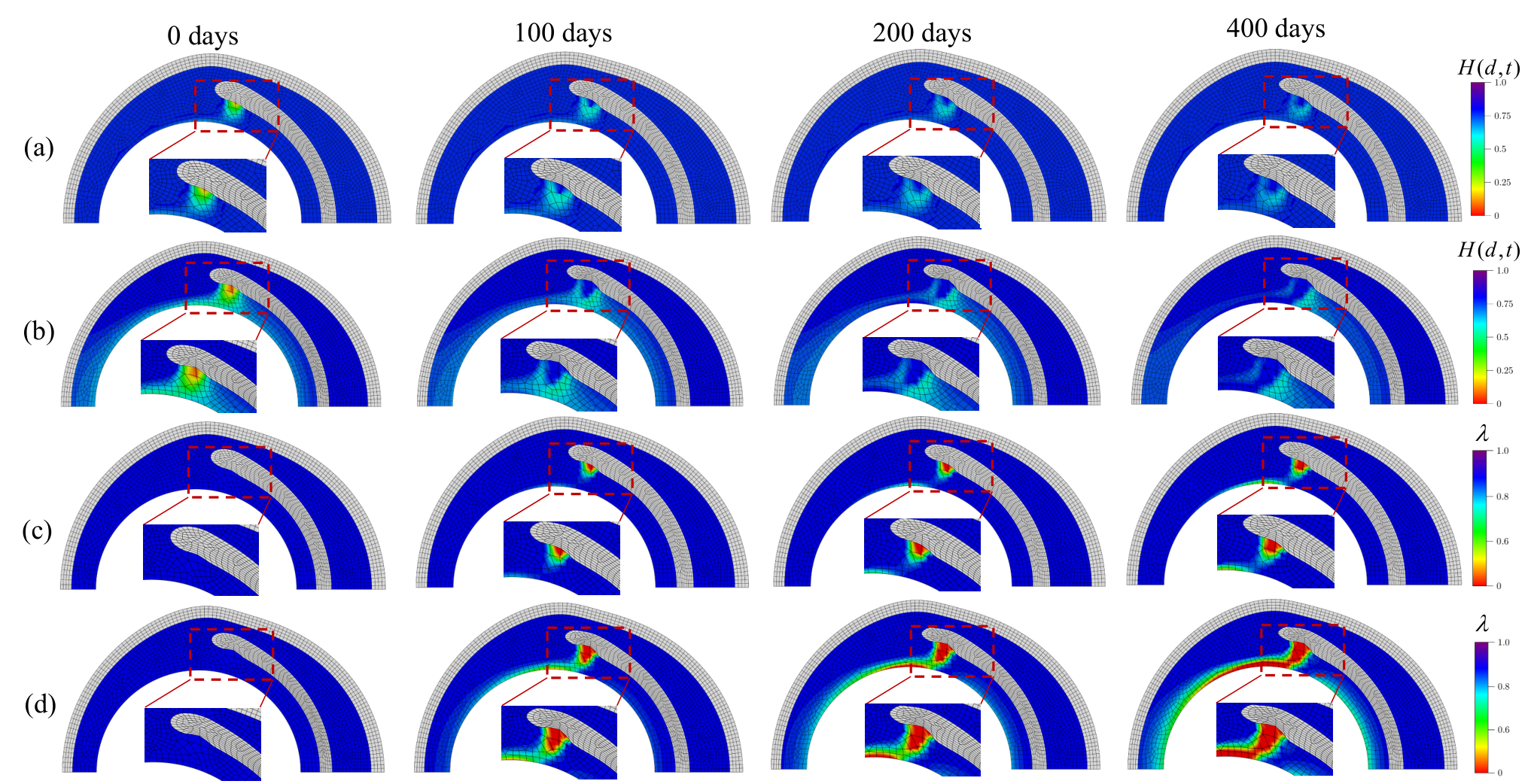
The performance of the proposed model is tested by simulating the variations in four healing related parameters, $H(d,t)$, $\lambda$, $F_{g1}(1,1)$ and $F_{g2}(1,1)$, as shown in Fig. 14. The results of $H(d,t)$ in Fig. 14(a) show that the damage initially mainly occurs at the fiber cap in the shoulder of the plaque, the results agree with the review report of Holzapfel et al. [23]. The variation of $H(d,t)$ from 0 day to 400 day shown in Fig. 14(a) demonstrates that the damage in balloon angioplasty can be partly healed over a long-term time, for instance, the minimum value of the healing parameter $H(d,t)$ in the entire domain is increasing from 0.46 to 0.83 in this example. Moreover, it is interesting that our proposed model provides the variations of more parameters during the healing process at the same time, for instance, the results of $\lambda$ shown Fig. 14(b) indicates that the position where the new tissue is produced is almost the same with the position where the damage occurred. The component of the growth deformation for the original $F_{g1}(1,1)$ and the newly deposited tissues $F_{g2}(1,1)$ are also shown in Fig. 14(c) and Fig. 14(d), respectively, which illustrate the influence of growth on deformation in the healing process.

To further investigate the evolution of G&R at specific positions, four nodes (the locations shown in Fig. 13) are selected, and the Von Mises stress $\sigma_{m}$ and the magnitude of displacement $u_{m}=\sqrt{u_{x}^{2}+u_{y}^{2}}$ are calculated as shown in Fig. 15. The curves of the variations of $\sigma_{m}$ and $u_{m}$ with time shown in Fig. 15 illustrate that the proposed model works well and can converge to the homeostatic state.

As the inflation size is the critical indicator in balloon angioplasty [24], two inflation sizes are tested to investigate the influence of the inflation size on G&R, as the contours of the healing parameter $H(d,t)$ and the the volume ratio of the newly deposited part $\lambda$ are shown in Fig. 16. The minimum value of the healing parameter $H(d,t)$ at $[0,100,200,400]$ days is $[0.46,0.82,0.83,0.83]$ when $r_{f}=1.40\ \rm mm$ compared with the corresponding results of $H(d,t)$ is $[0.17,0.74,0.77,0.79]$ when $r_{f}=1.48\ \rm mm$. Although a faster healing speed can be observed at the beginning of the healing process when $r_{f}=1.48\ \rm mm$, a larger area of unrecoverable damage remains when healing is completed. Therefore, the long-term evolution of the damage is also important and must be considered. Fig. 17 shows the evolution of the normalized outer artery radius $R(t)$ in the healing process, obtained by calculating the time-dependent ratio of the outer radius of the artery $R(t)=\frac{r_{oa}(t)}{r_{oa}(t=0)}$, where $r_{oa}$ is the outer radius of the artery. The variations of $R(t)$ shown in Fig. 17 demonstrates that the artery wall gradually changes to be thicker during the healing process and finally converges to a stable thickness at homeostatic state, this phenomenon is similar to the computational results by Braeu et al. in simulating of the thickening of arterial wall in hypertension [25]. It can be explained that thickening of the wall helps restore a homeostatic state, as it decreases the wall stress back to the initial level [25]. A smaller deformation for $r_{f}=1.48\ \rm mm$ can be illustrated by a larger unrecoverable damage, which means that litter displacement is needed to recover to the homeostatic stress state, similar to the results in Example 2.

References

- Rao [2011] I. Rao, Modeling of growth and remodeling in soft biological tissues with multiple constituents, Mechanics Research Communications 38 (2011) 24–28.
- Gasser [2017] T. C. Gasser, Damage in Vascular Tissues and Its Modeling, Springer International Publishing, Cham, pp. 85–118.
- Valero et al. [2015] C. Valero, E. Javierre, J. García-Aznar, M. Gómez-Benito, A. Menzel, Modeling of anisotropic wound healing, Journal of the Mechanics and Physics of Solids 79 (2015) 80–91.
- Comellas et al. [2016] E. Comellas, T. C. Gasser, F. J. Bellomo, S. Oller, A homeostatic-driven turnover remodelling constitutive model for healing in soft tissues, Journal of the Royal Society Interface 13 (2016) 20151081.
- Cumming et al. [2009] B. D. Cumming, D. McElwain, Z. Upton, A mathematical model of wound healing and subsequent scarring, Journal of The Royal Society Interface 7 (2009) 19–34.
- Buganza Tepole and Kuhl [2016] A. Buganza Tepole, E. Kuhl, Computational modeling of chemo-bio-mechanical coupling: a systems-biology approach toward wound healing, Computer methods in biomechanics and biomedical engineering 19 (2016) 13–30.
- Javierre et al. [2009] E. Javierre, P. Moreo, M. Doblaré, J. García-Aznar, Numerical modeling of a mechano-chemical theory for wound contraction analysis, International journal of solids and structures 46 (2009) 3597–3606.
- Schugart et al. [2008] R. C. Schugart, A. Friedman, R. Zhao, C. K. Sen, Wound angiogenesis as a function of tissue oxygen tension: a mathematical model, Proceedings of the National Academy of Sciences 105 (2008) 2628–2633.
- Kuhl et al. [2005] E. Kuhl, K. Garikipati, E. M. Arruda, K. Grosh, Remodeling of biological tissue: mechanically induced reorientation of a transversely isotropic chain network, Journal of the Mechanics and Physics of Solids 53 (2005) 1552–1573.
- Humphrey and Rajagopal [2002] J. Humphrey, K. Rajagopal, A constrained mixture model for growth and remodeling of soft tissues, Mathematical models and methods in applied sciences 12 (2002) 407–430.
- Latorre and Humphrey [2018] M. Latorre, J. D. Humphrey, Critical roles of time-scales in soft tissue growth and remodeling, APL bioengineering 2 (2018) 026108.
- Dimitrijevic and Hackl [2008] B. Dimitrijevic, K. Hackl, A method for gradient enhancement of continuum damage models, Technische Mechanik 28 (2008) 43–52.
- He et al. [2019] Y. He, D. Zuo, K. Hackl, H. Yang, S. J. Mousavi, S. Avril, Gradient-enhanced continuum models of healing in damaged soft tissues, Biomechanics and modeling in mechanobiology (2019) 1–18.
- Zuo et al. [2020] D. Zuo, S. Avril, H. Yang, S. J. Mousavi, K. Hackl, Y. He, Three-dimensional numerical simulation of soft-tissue wound healing using constrained-mixture anisotropic hyperelasticity and gradient-enhanced damage mechanics, Journal of the Royal Society Interface 17 (2020) 20190708.
- Frank et al. [1999a] C. B. Frank, N. G. Shrive, H. Hiraoka, N. Nakamura, Y. Kaneda, D. A. Hart, Optimisation of the biology of soft tissue repair, Journal of Science and Medicine in Sport 2 (1999a) 190–210.
- Frank et al. [1999b] C. B. Frank, D. A. Hart, N. G. Shrive, Molecular biology and biomechanics of normal and healing ligaments—a review, Osteoarthritis and Cartilage 7 (1999b) 130–140.
- Dimitrijevic and Hackl [2011] B. Dimitrijevic, K. Hackl, A regularization framework for damage–plasticity models via gradient enhancement of the free energy, International Journal for Numerical Methods in Biomedical Engineering 27 (2011) 1199–1210.
- Nolan et al. [2014] D. Nolan, A. Gower, M. Destrade, R. Ogden, J. McGarry, A robust anisotropic hyperelastic formulation for the modelling of soft tissue, Journal of the mechanical behavior of biomedical materials 39 (2014) 48–60.
- Waffenschmidt et al. [2014] T. Waffenschmidt, C. Polindara, A. Menzel, S. Blanco, A gradient-enhanced large-deformation continuum damage model for fibre-reinforced materials, Computer Methods in Applied Mechanics and Engineering 268 (2014) 801–842.
- Polindara et al. [2017] C. Polindara, T. Waffenschmidt, A. Menzel, A computational framework for modelling damage-induced softening in fibre-reinforced materials–application to balloon angioplasty, International Journal of Solids and Structures 118 (2017) 235–256.
- Loree et al. [1992] H. M. Loree, R. Kamm, R. Stringfellow, R. T. Lee, Effects of fibrous cap thickness on peak circumferential stress in model atherosclerotic vessels., Circulation research 71 (1992) 850–858.
- Gasser and Holzapfel [2007] T. C. Gasser, G. A. Holzapfel, Modeling plaque fissuring and dissection during balloon angioplasty intervention, Annals of biomedical engineering 35 (2007) 711–723.
- Holzapfel et al. [2014] G. A. Holzapfel, J. J. Mulvihill, E. M. Cunnane, M. T. Walsh, Computational approaches for analyzing the mechanics of atherosclerotic plaques: A review, Journal of Biomechanics 47 (2014) 859–869.
- Tenaglia et al. [1997] A. N. Tenaglia, et al., Intravascular ultrasound and balloon percutaneous transluminal coronary angioplasty, Cardiology clinics 15 (1997) 31–38.
- Braeu et al. [2017] F. Braeu, A. Seitz, R. Aydin, C. Cyron, Homogenized constrained mixture models for anisotropic volumetric growth and remodeling, Biomechanics and modeling in mechanobiology 16 (2017) 889–906.