Proxy Synthesis: Learning with Synthetic Classes for Deep Metric Learning
Abstract
One of the main purposes of deep metric learning is to construct an embedding space that has well-generalized embeddings on both seen (training) classes and unseen (test) classes. Most existing works have tried to achieve this using different types of metric objectives and hard sample mining strategies with given training data. However, learning with only the training data can be overfitted to the seen classes, leading to the lack of generalization capability on unseen classes. To address this problem, we propose a simple regularizer called Proxy Synthesis that exploits synthetic classes for stronger generalization in deep metric learning. The proposed method generates synthetic embeddings and proxies that work as synthetic classes, and they mimic unseen classes when computing proxy-based losses. Proxy Synthesis derives an embedding space considering class relations and smooth decision boundaries for robustness on unseen classes. Our method is applicable to any proxy-based losses, including softmax and its variants. Extensive experiments on four famous benchmarks in image retrieval tasks demonstrate that Proxy Synthesis significantly boosts the performance of proxy-based losses and achieves state-of-the-art performance.
1 Introduction
Deep metric learning aims to learn a similarity metric among arbitrary data points so that it defines an embedding space where semantically similar images are close together, and dissimilar images are far apart. Owing to its practical significance, it has been used for a variety of tasks such as image retrieval (Gordo et al. 2016; Sohn 2016), person re-identification (Yu et al. 2018; Hermans, Beyer, and Leibe 2017), zero-shot learning (Zhang and Saligrama 2016), and face recognition (Wen et al. 2016; Deng et al. 2019). The well-structured embedding is requested to distinguish the unseen classes properly, where the model is required to learn image representation from seen classes. This has been achieved by loss functions, which can be categorized into two types: pair-based and proxy-based loss.
The pair-based losses are designed based on the pair-wise similarity between data points in the embedding space, such as contrastive (Chopra, Hadsell, and LeCun 2005), triplet (Weinberger and Saul 2009), N-pair loss (Sohn 2016), etc. However, they require high training complexity and empirically suffer from sampling issues (Movshovitz-Attias et al. 2017). To address these issues, the concept of proxy has been introduced. A proxy is a representative of each class, which can be trained as a part of the network parameters. Given a selected data point as an anchor, proxy-based losses consider its relations with proxies. This alleviates the training complexity and sampling issues because only data-to-proxy relations are considered with a relatively small number of proxies compared to that of data points.
Although the performance of metric learning losses has been improved, a network trained only with training (seen) data can be overfitted to the seen classes and suffer from low generalization on unseen classes. To resolve this problem, previous works (Zheng et al. 2019; Gu and Ko 2020; Ko and Gu 2020) have generated synthetic samples to exploit additional training signals and more informative representations. However, these methods can only be used for pair-based losses; thus, they still suffer from the training complexity and sampling issues.
In this paper, we propose Proxy Synthesis (PS), which is a simple regularizer for proxy-based losses that encourages networks to construct better generalized embedding space for unseen classes. As illustrated in Figure 1, our method generates synthetic embeddings and proxies as synthetic classes for computing a proxy-based loss. Proxy Synthesis exploits synthetic classes generated by semantic interpolations to mimic unseen classes, obtaining smooth decision boundaries and an embedding space considering class relations. Moreover, the proposed method can be used with any proxy-based loss, including softmax loss and its variants. We demonstrate that our proposed method yields better robustness on unseen classes and deformation on the input and embedding feature. We achieve a significant performance boost on every proxy-based loss with Proxy Synthesis and obtain state-of-the-art performance with respect to four famous benchmarks in image retrieval tasks.
2 Related Work
Sample Generation:
To achieve better generalization, previous works (Zhao et al. 2018; Duan et al. 2018; Zheng et al. 2019) have leveraged a generative network to create synthetic samples, which can lead to a bigger model and slower training speed. To solve these problems, recent works (Gu and Ko 2020; Ko and Gu 2020) have proposed to generate samples by algebraic computation in the embedding space. However, the above works can only be used for pair-based losses, which causes the same drawbacks of high training complexity and careful pair mining. In addition, the above works exploit synthetic embeddings only for existing (seen) classes, when Proxy Synthesis uses synthetic embeddings and proxies as virtual classes for generalization on unseen classes explicitly.
Mixup:
Mixup techniques (Zhang et al. 2017; Verma et al. 2018; Guo, Mao, and Zhang 2019) have been proposed for generalization in the classification task. These techniques linearly interpolate a random pair of training samples and the corresponding one-hot labels. Proxy Synthesis and Mixup techniques share the common concept in terms of interpolating features for augmentation but have three major differences. First, Mixup techniques are proposed for generalization, which aims for robustness on seen classes, such as classification, whereas Proxy Synthesis is proposed for generalization in metric learning tasks, aiming for robustness on unseen classes. Second, Mixup techniques interpolate the input vectors and hidden representations, whereas the proposed method interpolates the embedding features in the output space. Third, Mixup techniques interpolate one-hot labels, while Proxy Synthesis interpolates proxies, which allow us to learn the positional relations of class representatives in the embedding space explicitly.
Virtual Class:
Virtual softmax (Chen, Deng, and Shen 2018) generates a single weight as a virtual negative class for softmax function to enhance the discriminative property of learned features in the classification task. Even though the work proves that the constrained region for each class becomes more compact by the number of classes increase, Virtual softmax considers a single synthetic weight without any corresponding embedding as a virtual negative class. Moreover, generating virtual weight by is not applicable for softmax variants with weight normalization (i.e. Norm-Softmax, ArcFace, Proxy-anchor, etc), where is -th embedding, and is its positive class weight. This is because of the synthetic negative class will be equivalent to after normalization. In contrast, Proxy Synthesis generates multiple proxies (weights) and corresponding embeddings as multiple virtual classes, which can be used as negative and also positive classes. Moreover, the proposed method is applicable for any proxy-based loss and softmax variants.
3 Proposed Method
3.1 Preliminary
Consider a deep neural network , which maps from an input data space to an embedding space . We define a set of embedding feature , where each feature has label of and is the number of embedding features. We denote a set of proxy and formulate generalized proxy-based loss as:
| (1) |
where denotes random pair of embedding and matching proxy from the pair distribution .
Softmax loss is not only the most widely used classification loss but also has been re-valued as competitive loss in metric learning (Zhai and Wu 2018; Boudiaf et al. 2020). Let denote the -th column of the weight , where is the size of embedding features. Then, Softmax loss is presented as follows:
| (2) |
where we set the bias because it does not affect the performance (Liu et al. 2017; Deng et al. 2019). Because the proxy is learned as model parameter, the weight of softmax loss can be interpreted as proxy, which is the center of each class (Deng et al. 2019; Wang et al. 2018b).
Normalizing the weights and feature vector is proposed to lay them on a hypersphere of a fixed radius for better interpretation and performance (Wang et al. 2017; Wang et al. 2018a; Liu et al. 2017). When we transform the logit (Pereyra et al. 2017) as and fix the individual proxy (weight) and feature by -normalization, the normalized softmax (Norm-softmax) loss can be written with proxy-wise form as:
| (3) |
where is a positive proxy, is a set of negative proxies, is a scale factor, and denotes the cosine similarity between and . More details of proxy-based (Proxy-NCA (Movshovitz-Attias et al. 2017), SoftTriple (Qian et al. 2019), and Proxy-anchor (Kim et al. 2020)) and softmax variants (SphereFace (Liu et al. 2017), ArcFace (Deng et al. 2019), and CosFace (Wang et al. 2018b)) losses are presented in the supplementary Section A.
3.2 Proxy Synthesis
One of the key purposes of metric learning is to construct a robust embedding space for unseen classes. For this purpose, the proposed method allows proxy-based losses to exploit synthetic classes. Training a proxy-based loss using Proxy Synthesis is performed in three steps. First, we process a mini-batch of input data with a network to obtain a set of embeddings . Second, given two random pairs of an embedding and corresponding proxy from different classes, and , we generate a pair of synthetic embedding and proxy as follows:
| (4) |
where is a linear interpolation function with the coefficient of for , and . We perform generations of Eq. 4, where hyper-parameter is a generation ratio by batch size. Thereafter, we define as a set of original and synthetic embeddings, and as a set of original and synthetic proxies. Synthetic proxy will work as a representative of the synthetic class, which has a mixed representation of class and , whereas the synthetic embedding will be a synthetic data point of the synthetic class. Third, we compute the loss, including synthetic embeddings and proxies, as if they are new classes. The generalized loss with Proxy Synthesis is formulated as:
| (5) |
where is a distribution of the embedding and proxy pairs including originals and synthetics generated with . Implementing Proxy Synthesis is extremely simple with few lines of codes. Moreover, it does not require to modify any code of proxy-based loss and can be used in a plug-and-play manner with negligible computation cost. Code-level description and experiment of training time and memory are presented in the supplementary Section B.1 and D.1, respectively.
3.3 Discussion
Learning with Class Relations:
Unlike tasks that only test with seen classes such as classification, metric learning is desired to construct a structural embedding space for robustness on unseen classes. A well-structured embedding space should contain meaningful relations among embeddings; an example from the previous work (Mikolov et al. 2013) is as follows: in a word embedding space. To achieve this, Proxy Synthesis explicitly inserts in-between class relations with synthetic classes (i.e., ) and they mimic unseen classes for training with a diverse range of data characteristics. Proxy Synthesis considers class relations with Equation 4 and 5 in forward propagation. This characteristic is reflected in backward propagation as well.
For convenience in gradient analysis, we write the loss of softmax function on , where is an anchor embedding of input, and is corresponding positive proxy, as follows,
| (6) |
where and . Then, gradient over positive similarity is,
| (7) |
It shows that the gradient over only considers the similarity of the anchor embedding and its proxy by .
When Proxy Synthesis is applied, the gradient changes. In this gradient induction, we assume that the positive proxy of input is used for generating synthesized proxy with as , where . Then, the gradients over and are inducted as follows,
| (8) | |||||
| (9) |
In contrast to the softmax loss, Proxy Synthesis enables the gradient over and to consider class relation between and via in the backward propagation. The detailed induction is presented in supplementary Section B.2.
Obtaining a Smooth Decision Boundary:
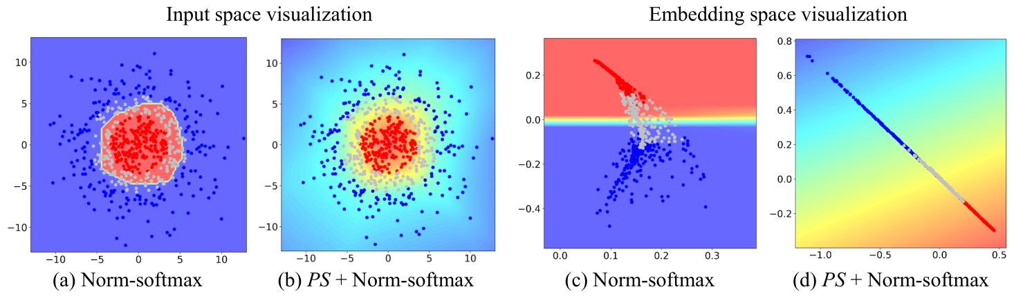
Synthetic classes work as hard competitors of original classes because of positional proximity, which leads to lower prediction confidence and, thus, smoother decision boundaries. The smoothness of the decision boundary is a main factor of generalization (Bartlett and Shawe-Taylor 1999; Verma et al. 2018), and it is more desirable in metric learning to provide a relaxed estimate of uncertainty for unseen classes. For better intuitions, we conduct an experiment to visualize the generalization effect of Proxy Synthesis, as depicted in Figure 2. For both the input and embedding spaces, Norm-softmax has a strict decision boundary, whereas PS + Norm-softmax has a smooth decision boundary that transitions linearly from the red to the blue class. Further theoretical analysis of such phenomenon is provided below.
A network with ordinary softmax outputs the probability of an embedding belonging to a specific class as follows,
| (10) |
Considering the linearity of similarity function , the strict decision boundary is constructed when the network always outputs embedding vector close to one proxy, even though the input has shared visual semantics among different classes. Such phenomenon occurs because the softmax function forces all embedding vectors to become as close to the corresponding proxies as possible during training. Considering the softmax loss of an embedding vector and its positive proxy as Equation 6, the gradient of such loss over can be inducted as follows:
| (11) | |||||
| , | (12) |
It is obvious that and . Considering the parameter update is performed by , where is a learning rate, the gradient descent forces to be closer to and to be distant from other proxies .
Proxy Synthesis overcomes such problem of embedding space to overfit to the proxies by providing a gradient of opposite direction compared to ordinary softmax. To describe major difference of Proxy Synthesis and ordinary softmax, we consider softmax loss for synthesized pair , where and are pairs of an embedding and a corresponding proxy:
| (13) | |||||
where and . It should be noted that . Since we suggest to sample from with small in Section 4.3, has high chance to be generated either close to with or close to with . As the proofs for both cases are equivalent, we assume the first case: is much closer to than . We consider gradient over because the loss will affect the closer embedding vector more than the other one. The inducted gradient over is as follows:
| (14) |
As is closer to and compared to other proxies, . Thus, Equation 14 can be re-written as follows,
| (15) | |||
| (16) |
It is obvious that , implying that by adopting Proxy Synthesis, softmax loss for synthesized pair provides gradient which leads embedding vector not too close to the corresponding proxy ; it is also obvious that , implying that softmax loss for synthesized pair provides gradient which makes embedding vector not too distant from the competing proxy . In such a manner, Proxy Synthesis prevents embedding vectors lying too close to proxies, which finally leads to the smooth decision boundary. The detailed induction is provided in the supplementary Section B.3.

4 Experiments
4.1 Experimental Setting
We evaluate the proposed method with respect to four benchmarks in metric learning: CUB-200-2011 (CUB200) (Wah et al. 2011), CARS196 (Krause et al. 2013), Standford Online Products (SOP) (Oh Song et al. 2016), and In-Shop Clothes (In-Shop) (Liu et al. 2016). We follow the widely used training and evaluation procedure from (Oh Song et al. 2016; Kim et al. 2020) and call it conventional evaluation. Experiments are performed on an Inception network with batch normalization (Ioffe and Szegedy 2015) with a 512 embedding dimension. For the hyper-parameters of Proxy Synthesis, and are set to 0.4 and 1.0, respectively. Considering recent works (Musgrave, Belongie, and Lim 2020; Fehervari, Ravichandran, and Appalaraju 2019) that have presented enhanced evaluation procedure with regard to fairness, we include an evaluation procedure designed from work “A metric learning reality check” (Musgrave, Belongie, and Lim 2020) and call it MLRC evaluation, which contains 4-fold cross-validation, ensemble evaluation, and usage of fair metrics (P@1, RP, and MAP@R). Please refer to supplementary Section C for further details on the benchmarks and implementation.
Model Embedding Proxy R@1 Original Synthetic Original Synthetic M1 (baseline) ✓ ✓ 83.3 M2 ✓ ✓ 83.1 M3 ✓ ✓ ✓ 83.7 M4 ✓ ✓ ✓ 83.7 Proxy Synthesis ✓ ✓ ✓ ✓ 84.7
4.2 Impact of Synthetic Class
Embedding Space Visualization:
Exploiting synthetic classes is preferable in metric learning because the main goal is to develop robustness on unseen classes. This is depicted visually in Figure 3. In Figure 3a, unseen test embeddings are located in-between the clusters of train embeddings by forming clusters. Similarly, synthetic classes are also generated in-between train embeddings, as depicted in Figure 3b, and play an important role in mimicking unseen classes during the training phase. Thus, these additional training signals enable a network to capture extra discriminative features for better robustness on unseen classes. Extended visualization is in supplementary Section D.5.
Impact of Synthetic Embedding and Proxy:
To investigate the quantitative impact of synthetic embedding and proxy, we conduct an experiment by differentiating the elements of and in Norm-softmax loss. Table 1 illustrates that using only synthetic embeddings and proxies (M2) leads to a slightly lower performance than the baseline (M1). Adding synthetic proxies (M3) and using synthetic embedding instead of the original embedding (M4) leads to improved performance when compared with the baseline (M1). This indicates that the generated synthetic embeddings and proxies build meaningful virtual classes for training. Finally, using all embeddings and proxies (Proxy Synthesis) achieves the best performance among all cases by considering the fundamental and additional training signals.
R@1(%) 0.1 83.1 0.2 83.8 0.3 83.7 0.4 83.5 0.5 83.3
R@1(%) 0.2 84.0 0.4 84.7 0.8 83.9 1.0 83.7 1.5 83.7

4.3 Synthetic Class as Hard Competitor
Impact of Hardness:
Generating synthetic classes is required to be hard enough so that the model can learn more discriminative representations. The hardness of synthetic classes can be controlled by , which decides probability distribution for the sampling of the interpolation coefficient . In Table 2, static shows low performance because synthetic classes are too close to original classes, and static also shows low performance because it generates synthetic classes in the middle of two original classes, which is relatively easy to distinguish. The optimal static value is around 0.2, which establishes the proper difficulty of distinguishment. Moreover, the result shows that the stochastic generation is better than the static generation. This is because stochastic generation can generate more number of different synthetic classes with wide variation. In the stochastic generation, is the same with uniform distribution, and has a high chance of generating synthetics in the middle of two classes; thus, their performance is relatively low. Similar to the experiment of static generation, around shows the best performance, which has a high chance of generating synthetic classes close enough to an original class. We provide additional experiments on the effect of hyper-parameter in supplementary Section D.2.
Logits Visualization:
We compare the cosine similarity (logits) between embeddings and proxies during the training procedure. In Figure 4a, the logit values of ground truth (GT), which are represented by the main diagonal , are clearly red owing to high prediction confidence. This leads to a strict decision boundary, as depicted in Figure 2a and Figure 2c, and may cause an overfitting problem. On the other hand, the GT logit values of PS + Norm-softmax ( and ) have lower confidence, represented with yellow to orange color. This is because synthetic classes generated near the original classes work as hard competitors ( and ), which prevents excessively high confidence, while the confidence of main diagonals ( and ) is still higher than that of competitors’ diagonals ( and ) with redder color for the same embedding. This smoothens the decision boundary, as depicted in Figure 2b and Figure 2d, and leads to stronger generalization.
Deformation Norm-softmax PS + Norm-softmax Cutout 75.3 77.0 (+1.7) Dropout 59.7 62.2 (+2.5) Zoom in 64.3 65.6 (+1.3) Zoom out 78.3 80.0 (+1.7) Rotation 70.8 72.1 (+1.3) Shearing 70.3 72.0 (+1.7) Gaussian noise 65.1 67.2 (+2.1) Gaussian blur 74.4 76.3 (+1.9)


CUB200 CARS196 SOP Loss P@1 RP MAP@R P@1 RP MAP@R P@1 RP MAP@R Norm-softmax 65.65 0.30 35.99 0.15 25.25 0.13 83.16 0.25 36.20 0.26 26.00 0.30 75.67 0.17 50.01 0.22 47.13 0.22 PS + Norm-softmax 69.19 0.34 37.32 0.29 26.40 0.29 85.70 0.24 38.33 0.31 28.31 0.32 76.73 0.15 51.46 0.21 48.52 0.20 CosFace 67.32 0.32 37.49 0.21 26.70 0.23 85.52 0.24 37.32 0.28 27.57 0.30 75.79 0.14 49.77 0.19 46.92 0.19 PS + CosFace 69.52 0.26 37.99 0.23 27.10 0.23 85.58 0.27 38.01 0.19 27.89 0.20 76.89 0.20 51.60 0.31 48.68 0.33 ArcFace 67.50 0.25 37.31 0.21 26.45 0.20 85.44 0.28 37.02 0.29 27.22 0.30 76.20 0.27 50.27 0.38 47.41 0.40 PS + ArcFace 68.79 0.31 37.46 0.26 26.79 0.27 85.59 0.25 38.31 0.22 28.24 0.20 77.21 0.20 51.90 0.23 49.02 0.21 SoftTriple 67.73 0.39 37.34 0.19 26.51 0.20 84.49 0.26 37.03 0.21 28.07 0.21 76.12 0.17 50.21 0.18 47.35 0.19 PS + SoftTriple 68.26 0.16 37.98 0.21 27.02 0.21 85.53 0.12 38.40 0.20 28.45 0.19 77.59 0.26 52.45 0.21 49.53 0.23 Proxy-NCA 65.69 0.43 35.14 0.26 24.21 0.27 83.56 0.27 35.62 0.28 25.38 0.31 75.89 0.17 50.10 0.22 47.22 0.21 PS + Proxy-NCA 66.02 0.29 35.73 0.24 24.84 0.22 84.61 0.19 36.39 0.25 26.04 0.27 76.78 0.21 51.39 0.27 48.44 0.27 Proxy-anchor 69.73 0.31 38.23 0.37 27.44 0.35 86.20 0.21 39.08 0.31 29.37 0.29 75.37 0.15 50.19 0.14 47.25 0.15 PS + Proxy-anchor 70.41 0.36 38.82 0.29 28.11 0.29 86.90 0.35 39.38 0.27 29.71 0.25 75.52 0.21 50.45 0.22 47.49 0.20
Regularizer Softmax Norm-softmax CARS196 SOP CARS196 SOP Baseline 81.5 76.3 83.3 78 Virtual Softmax 77.3 (-4.2) 76.2 (-0.1) - - Input Mixup 81.1 (-0.4) 77.0 (+0.7) 82.2 (-1.1) 78.2 (+0.2) Manifold Mixup 81.6 (+0.1) 77.5 (+1.2) 83.6 (+0.3) 78.4 (+0.4) Proxy Synthesis 84.3 (+2.8) 78.1 (+1.8) 84.7 (+1.4) 79.6 (+1.6)
4.4 Robustness to Deformation
Input Deformation:
To further evaluate the quality of representations learned with Proxy Synthesis, we perform a deformation test on the input data with trained networks. In Table 3, we evaluate the test data with several input deformations that are not used in training. A better-generalized model should be more robust to a large variety of input deformations. The result indicates that the network trained using Proxy Synthesis demonstrates significantly improved performance to input deformations.
Embedding Deformation:
To see the robustness on embedding deformation of trained networks, we evaluate performance with synthetic embeddings. Figure 5 depicts a network trained with Norm-softmax loss struggling with low performance on both the train and test set. In contrast, a network trained with Proxy Synthesis performs almost twice as well when compared with Norm-softmax loss on both the train and test set. This demonstrates that Proxy Synthesis provides more robust embedding features, which also leads to robustness on unseen classes. Besides, the patterns of performance are similar to those discussed in Section 4.3. When is close to 0 and 1, the performance is low because of hard synthetics, and when is close to 0.5, the performance is high because of relatively easy synthetics. Additional experiments are in the supplementary Section D.3.
4.5 Comparison with Other Regularizers
Further, we compare the proposed method with other regularizers, including Virtual Softmax, Input Mixup, and Manifold Mixup in the image retrieval task. Note that Virtual Softmax is not applicable to Norm-softmax loss because will always be constant . As presented in Table 5, Virtual Softmax degrades the performance of all cases with a margin of average -2.15%. Input Mixup degrades the performance on CARS196 with an average margin -0.75% and improves the performance on SOP with an average margin +0.45%. Manifold Mixup increases the performance of all cases with an average margin +0.5%. This illustrates that although these techniques are powerful for generalizing seen classes, such as classification tasks, they lack discriminative ability on unseen classes. On the other hand, Proxy Synthesis improves performance for all cases with a large margin of average +1.9% and achieves the best performance among all. Further analysis, including hyper-parameter search for Mixup and experiments in the classification task, is presented in the supplementary material Section D.4.
Method CUB200 CARS196 SOP In-Shop Softmax 64.2 81.5 76.3 90.4 PS + Softmax 64.9 (+0.7) 84.3 (+2.8) 77.6 (+1.3) 90.9 (+0.5) Norm-softmax 64.9 83.3 78.6 90.4 PS + Norm-softmax 66.0 (+1.1) 84.7 (+1.4) 79.6 (+1.0) 91.5 (+1.1) SphereFace 65.4 83.6 78.9 90.3 PS + SphereFace 66.6 (+1.2) 85.1 (+1.5) 79.4 (+0.5) 91.6 (+1.3) CosFace 65.7 83.6 78.6 90.7 PS + CosFace 66.6 (+0.9) 84.6 (+1.0) 79.3 (+0.7) 91.4 (+0.7) ArcFace 66.1 83.7 78.8 91.0 PS + ArcFace 66.8 (+0.7) 84.7 (+1.0) 79.7 (+0.9) 91.7 (+0.7) Proxy-NCA 65.1 83.7 78.1 90.0 PS + Proxy-NCA 66.4 (+1.3) 84.5 (+0.8) 79.1 (+1.0) 91.4 (+1.4) SoftTriple 65.4 84.5 78.3 91.1 PS + SoftTriple 66.6 (+1.2) 85.3 (+0.8) 79.5 (+1.2) 91.8 (+0.7) Proxy-anchor† 68.4 86.1 79.1 91.5 PS + Proxy-anchor† 69.2 (+0.8) 86.9 (+0.8) 79.8 (+0.7) 91.9 (+0.4)
4.6 Comparison with State-of-the-Art
Finally, we compare the performance of our proposed method with state-of-the-art losses in two ways: conventional and MLRC evaluation. In conventional evaluation, the combinations of Proxy Synthesis with proxy-based losses improve performance by a large margin in every benchmark as presented in Table 6. For fine-grained datasets with few categories such as CUB200 and CARS196, the performance gain ranges between a minimum of +0.7% and a maximum of +2.8%, and the average improvement is +1.1%. For large-scale datasets with numerous categories such as SOP and In-Shop, the performance gain ranges between a minimum of +0.4% and a maximum of +1.4%, and the average improvement is +0.9%. Even in the specifically designed MLRC evaluation, Table 4 shows that Proxy Synthesis enhances performance for every metric and benchmark. Extended comparisons with Recall@k for conventional evaluation and performance of seperated 128-dim for MLRC evaluation are presented in the supplementary Section D.6.
5 Conclusion
In this paper, we have proposed a novel regularizer called Proxy Synthesis for proxy-based losses that exploits synthetic classes for stronger generalization. Such effect is achieved by deriving class relations and smoothened decision boundaries. The proposed method provides a significant performance boost for all proxy-based losses and achieves state-of-the-art performance in image retrieval tasks.
Acknowledgement
We would like to thank Yoonjae Cho, Hyong-Keun Kook, Sanghyuk Park, Minchul Shin and Tae Kwan Lee from NAVER/LINE Vision team for helpful comments and feedback.
References
- Bartlett and Shawe-Taylor (1999) Bartlett, P.; and Shawe-Taylor, J. 1999. Generalization performance of support vector machines and other pattern classifiers. Advances in Kernel methods—support vector learning 43–54.
- Boudiaf et al. (2020) Boudiaf, M.; Rony, J.; Ziko, I. M.; Granger, E.; Pedersoli, M.; Piantanida, P.; and Ayed, I. B. 2020. A unifying mutual information view of metric learning: cross-entropy vs. pairwise losses. arXiv preprint arXiv:2003.08983 .
- Chen, Deng, and Shen (2018) Chen, B.; Deng, W.; and Shen, H. 2018. Virtual class enhanced discriminative embedding learning. In Advances in Neural Information Processing Systems, 1942–1952.
- Chopra, Hadsell, and LeCun (2005) Chopra, S.; Hadsell, R.; and LeCun, Y. 2005. Learning a similarity metric discriminatively, with application to face verification. In 2005 IEEE Computer Society Conference on Computer Vision and Pattern Recognition (CVPR’05), volume 1, 539–546. IEEE.
- Deng et al. (2019) Deng, J.; Guo, J.; Xue, N.; and Zafeiriou, S. 2019. Arcface: Additive angular margin loss for deep face recognition. In Proceedings of the IEEE Conference on Computer Vision and Pattern Recognition, 4690–4699.
- Duan et al. (2018) Duan, Y.; Zheng, W.; Lin, X.; Lu, J.; and Zhou, J. 2018. Deep adversarial metric learning. In Proceedings of the IEEE Conference on Computer Vision and Pattern Recognition, 2780–2789.
- Fehervari, Ravichandran, and Appalaraju (2019) Fehervari, I.; Ravichandran, A.; and Appalaraju, S. 2019. Unbiased evaluation of deep metric learning algorithms. arXiv preprint arXiv:1911.12528 .
- Gordo et al. (2016) Gordo, A.; Almazán, J.; Revaud, J.; and Larlus, D. 2016. Deep image retrieval: Learning global representations for image search. In European conference on computer vision, 241–257. Springer.
- Gu and Ko (2020) Gu, G.; and Ko, B. 2020. Symmetrical Synthesis for Deep Metric Learning. In Proceedings of the AAAI Conference on Artificial Intelligence.
- Guo, Mao, and Zhang (2019) Guo, H.; Mao, Y.; and Zhang, R. 2019. Mixup as locally linear out-of-manifold regularization. In Proceedings of the AAAI Conference on Artificial Intelligence, volume 33, 3714–3722.
- Hermans, Beyer, and Leibe (2017) Hermans, A.; Beyer, L.; and Leibe, B. 2017. In defense of the triplet loss for person re-identification. arXiv preprint arXiv:1703.07737 .
- Ioffe and Szegedy (2015) Ioffe, S.; and Szegedy, C. 2015. Batch normalization: Accelerating deep network training by reducing internal covariate shift. arXiv preprint arXiv:1502.03167 .
- Kim et al. (2020) Kim, S.; Kim, D.; Cho, M.; and Kwak, S. 2020. Proxy Anchor Loss for Deep Metric Learning. arXiv preprint arXiv:2003.13911 .
- Ko and Gu (2020) Ko, B.; and Gu, G. 2020. Embedding Expansion: Augmentation in Embedding Space for Deep Metric Learning. In Proceedings of the IEEE Conference on Computer Vision and Pattern Recognition.
- Krause et al. (2013) Krause, J.; Stark, M.; Deng, J.; and Fei-Fei, L. 2013. 3d object representations for fine-grained categorization. In Proceedings of the IEEE international conference on computer vision workshops, 554–561.
- Liu et al. (2017) Liu, W.; Wen, Y.; Yu, Z.; Li, M.; Raj, B.; and Song, L. 2017. Sphereface: Deep hypersphere embedding for face recognition. In Proceedings of the IEEE conference on computer vision and pattern recognition, 212–220.
- Liu et al. (2016) Liu, Z.; Luo, P.; Qiu, S.; Wang, X.; and Tang, X. 2016. Deepfashion: Powering robust clothes recognition and retrieval with rich annotations. In Proceedings of the IEEE conference on computer vision and pattern recognition, 1096–1104.
- Maaten and Hinton (2008) Maaten, L. v. d.; and Hinton, G. 2008. Visualizing data using t-SNE. Journal of machine learning research 9(Nov): 2579–2605.
- Mikolov et al. (2013) Mikolov, T.; Chen, K.; Corrado, G.; and Dean, J. 2013. Efficient estimation of word representations in vector space. arXiv preprint arXiv:1301.3781 .
- Movshovitz-Attias et al. (2017) Movshovitz-Attias, Y.; Toshev, A.; Leung, T. K.; Ioffe, S.; and Singh, S. 2017. No fuss distance metric learning using proxies. In Proceedings of the IEEE International Conference on Computer Vision, 360–368.
- Musgrave, Belongie, and Lim (2020) Musgrave, K.; Belongie, S.; and Lim, S.-N. 2020. A Metric Learning Reality Check. arXiv preprint arXiv:2003.08505 .
- Oh Song et al. (2016) Oh Song, H.; Xiang, Y.; Jegelka, S.; and Savarese, S. 2016. Deep metric learning via lifted structured feature embedding. In Proceedings of the IEEE conference on computer vision and pattern recognition, 4004–4012.
- Pereyra et al. (2017) Pereyra, G.; Tucker, G.; Chorowski, J.; Kaiser, Ł.; and Hinton, G. 2017. Regularizing neural networks by penalizing confident output distributions. arXiv preprint arXiv:1701.06548 .
- Qian et al. (2019) Qian, Q.; Shang, L.; Sun, B.; Hu, J.; Li, H.; and Jin, R. 2019. SoftTriple Loss: Deep Metric Learning Without Triplet Sampling. In Proceedings of the IEEE International Conference on Computer Vision, 6450–6458.
- Sohn (2016) Sohn, K. 2016. Improved deep metric learning with multi-class n-pair loss objective. In Advances in neural information processing systems, 1857–1865.
- Verma et al. (2018) Verma, V.; Lamb, A.; Beckham, C.; Najafi, A.; Mitliagkas, I.; Courville, A.; Lopez-Paz, D.; and Bengio, Y. 2018. Manifold mixup: Better representations by interpolating hidden states. arXiv preprint arXiv:1806.05236 .
- Wah et al. (2011) Wah, C.; Branson, S.; Welinder, P.; Perona, P.; and Belongie, S. 2011. The caltech-ucsd birds-200-2011 dataset .
- Wang et al. (2018a) Wang, F.; Cheng, J.; Liu, W.; and Liu, H. 2018a. Additive margin softmax for face verification. IEEE Signal Processing Letters 25(7): 926–930.
- Wang et al. (2017) Wang, F.; Xiang, X.; Cheng, J.; and Yuille, A. L. 2017. Normface: L2 hypersphere embedding for face verification. In Proceedings of the 25th ACM international conference on Multimedia, 1041–1049.
- Wang et al. (2018b) Wang, H.; Wang, Y.; Zhou, Z.; Ji, X.; Gong, D.; Zhou, J.; Li, Z.; and Liu, W. 2018b. Cosface: Large margin cosine loss for deep face recognition. In Proceedings of the IEEE Conference on Computer Vision and Pattern Recognition, 5265–5274.
- Weinberger and Saul (2009) Weinberger, K. Q.; and Saul, L. K. 2009. Distance metric learning for large margin nearest neighbor classification. Journal of Machine Learning Research 10(Feb): 207–244.
- Wen et al. (2016) Wen, Y.; Zhang, K.; Li, Z.; and Qiao, Y. 2016. A discriminative feature learning approach for deep face recognition. In European conference on computer vision, 499–515. Springer.
- Yu et al. (2018) Yu, R.; Dou, Z.; Bai, S.; Zhang, Z.; Xu, Y.; and Bai, X. 2018. Hard-aware point-to-set deep metric for person re-identification. In Proceedings of the European Conference on Computer Vision (ECCV), 188–204.
- Zhai and Wu (2018) Zhai, A.; and Wu, H.-Y. 2018. Classification is a Strong Baseline for Deep Metric Learning. arXiv preprint arXiv:1811.12649 .
- Zhang et al. (2017) Zhang, H.; Cisse, M.; Dauphin, Y. N.; and Lopez-Paz, D. 2017. mixup: Beyond empirical risk minimization. arXiv preprint arXiv:1710.09412 .
- Zhang and Saligrama (2016) Zhang, Z.; and Saligrama, V. 2016. Zero-shot learning via joint latent similarity embedding. In proceedings of the IEEE Conference on Computer Vision and Pattern Recognition, 6034–6042.
- Zhao et al. (2018) Zhao, Y.; Jin, Z.; Qi, G.-j.; Lu, H.; and Hua, X.-s. 2018. An adversarial approach to hard triplet generation. In Proceedings of the European conference on computer vision (ECCV), 501–517.
- Zheng et al. (2019) Zheng, W.; Chen, Z.; Lu, J.; and Zhou, J. 2019. Hardness-aware deep metric learning. In Proceedings of the IEEE Conference on Computer Vision and Pattern Recognition, 72–81.
See pages 1- of Proxy_synthesis_supp.pdf