Fundamental Challenges in Deep Learning for Stiff Contact Dynamics
Abstract
Frictional contact has been extensively studied as the core underlying behavior of legged locomotion and manipulation, and its nearly-discontinuous nature makes planning and control difficult even when an accurate model of the robot is available. Here, we present empirical evidence that learning an accurate model in the first place can be confounded by contact, as modern deep learning approaches are not designed to capture this non-smoothness. We isolate the effects of contact’s non-smoothness by varying the mechanical stiffness of a compliant contact simulator. Even for a simple system, we find that stiffness alone dramatically degrades training processes, generalization, and data-efficiency. Our results raise serious questions about simulated testing environments which do not accurately reflect the stiffness of rigid robotic hardware. Significant additional investigation will be necessary to fully understand and mitigate these effects, and we suggest several avenues for future study.
I INTRODUCTION
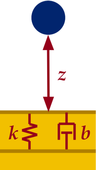
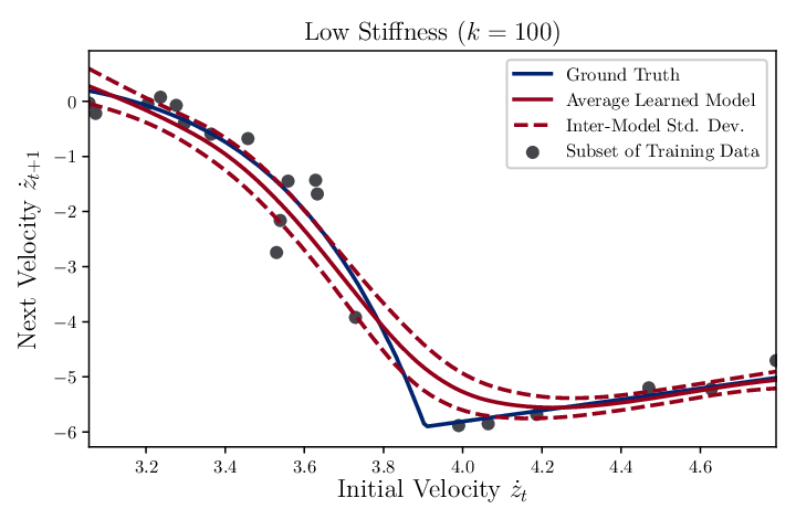

Advances in model-based control and planning have always been essential to state-of-the-art robotic manipulation and locomotion. Traditionally, roboticists have relied on high-accuracy, physics-based models of tightly-controlled laboratory environments. However, as robotic systems transition to practical applications in unknown and unstructured environments, learning accurate models from limited data becomes increasingly important. Despite recent successes leveraging modern deep learning to this end (e.g. [1, 2, 3, 4]), robotic performance remains decidedly sub-human in almost all scenarios. One limiting factor is that contact is challenging to leverage, even given an accurate model; controlling the nearly-discontinuous behaviors of impact remains incredibly difficult, despite extensive study [5]. In this work, we show the same properties also seriously impede common deep learning methods from obtaining an accurate model in the first place.
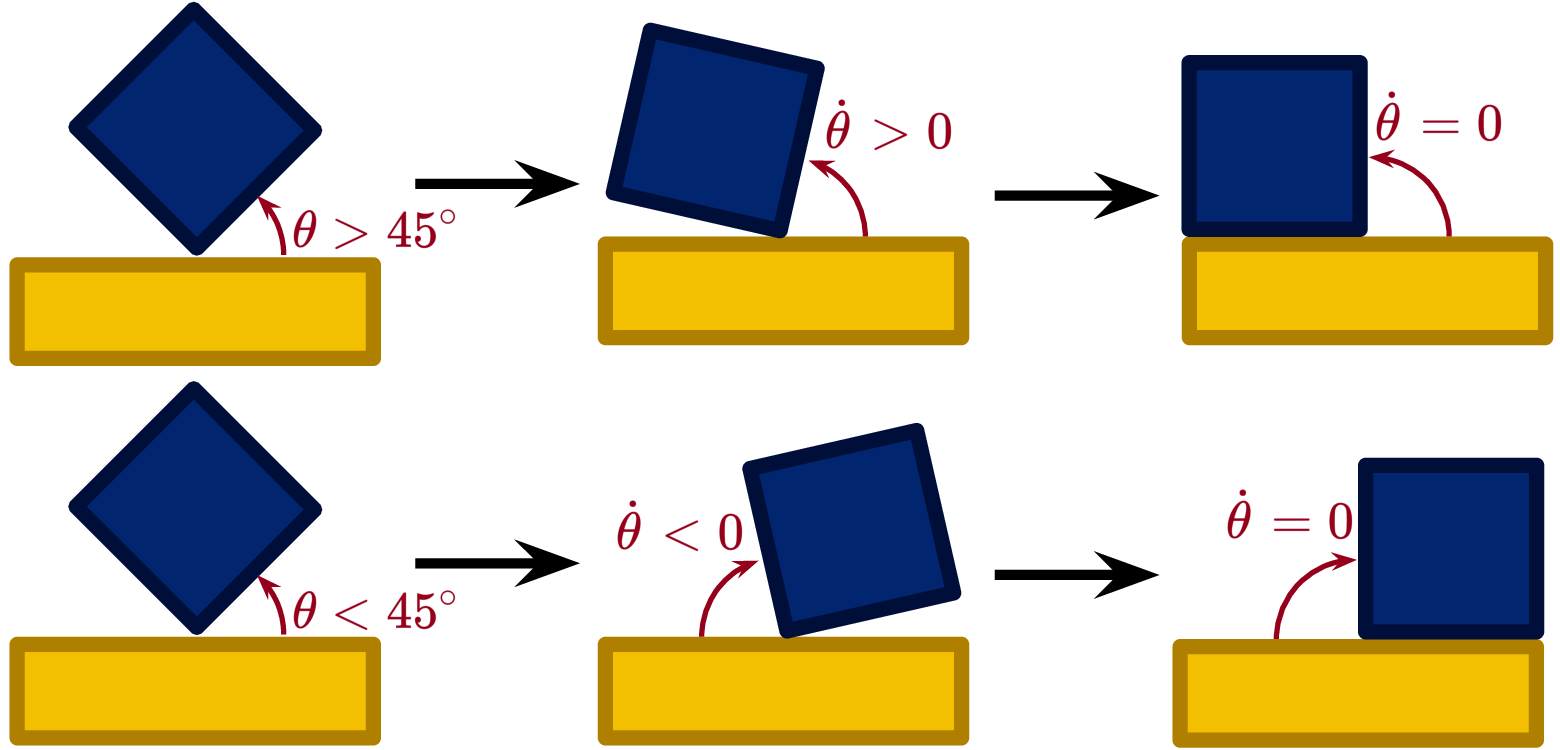
Impacts among robots and their surroundings are particularly difficult to model. When objects collide, materials deform on an imperceptibly small spatial and temporal scale, preventing interpenetration. The underlying material property driving this rapidity, mechanical stiffness, causes multiple forms of numerical stiffness in the equations of motion of these systems (See Figure 2). Slight inaccuracies in either initial conditions or model parameters can generate wildly-different predictions, even over a small time horizon [6, 7]. Furthermore, measurements of the velocities are extremely sensitive to the time that they are recorded, as they change near-instantaneously during impact [8, 9]. These properties become significant problems when learning a model of a real system from noisy sensor measurements.
Several associated issues have been duly noted in prior works on system identification (sysID) [10, 8] and differentiable physics [11, 12]. In these settings, a handful of unknown parameters of a physics-based model are fit to data. However, constructing an appropriate model space requires extensive knowledge of the robot and its surroundings; fitting model parameters requires expertise in both mechanics and optimization; and even excellent implementations are limited by inaccurate approximations, such as object rigidity and inelastic impact, inherent to tractable physical models [13].
The flexibility of deep neural networks (DNN’s) can circumvent each of these issues, but they also introduce challenges unique to their high-dimensional optimization setting. First, stiffness in the learned dynamics introduce both stiffness and local minima into the training optimization landscape [10, 11]. While sysID methods address this issue by exploiting either second-order [10] or global [11] optimization techniques, these tools cannot be tractably applied to the high-dimensional parameter spaces of DNN’s. Furthermore, while a fundamental advantage of DNN’s is their ability to approximate any dynamical system, a corresponding challenge is that many distinct model parameters may fit the training data well, and one must be selected via an inductive bias. Unfortunately, in direct conflict with the stiff and nearly-discontinuous behaviors of frictional contact, deep learning techniques tend to select the smoothest interpolator of the data. This behavior is both a predisposition of common training techniques like stochastic gradient descent (SGD) [14, 15] and an explicit goal of common regularizers such as weight-decay and spectral normalization [16, 17]. This smoothing effect is particularly harmful when available data is sparse, as can be see in a 1D example in Figure 1. If stiffness indeed significantly influences the performance of deep learning, then serious questions must be raised not only about robotic learning methods, but also the relevance of simulated results to the robotics community. Many simulators (e.g. MuJoCo [18]) allow users to specify mechanical stiffness; properly used, simulation can produce physically-accurate behaviors [10, 19]. However, ubiquitous benchmarking suites often use software default values for stiffness, rather than values tuned for realism [20]. The idea that unrealistic contact settings can generate a gap between simulated and real-world performance is an existing intuition in the robotics community [21]. However, this phenomenon has not been rigorously examined in the literature.
In this paper, we contribute an empirical quantification and isolation of the detrimental effects of stiffness on deep learning performance. We begin by describing how stiffness enters into the equations of motion of a simple simulated system in MuJoCo in Section II, and show that default settings are significantly less stiff than many real systems. In Section III, we propose a testing methodology to examine the negative effects of stiffness on inherent unpredictability, training process degradation, generalization, and long-term prediction. As is common intuition, our results (Section IV) show that raising stiffness degrades ground-truth model predictions as the underlying system becomes more sensitive to noise. However, we find that stiffness induces multiple pathological behaviors beyond this effect:
- 1.
The training error of learned models degrades with stiffness nearly twice as fast as the ground-truth model, even for single-step predictions.
- 2.
While generalization error can be eliminated for non-stiff systems with ample training data, test error stays significantly higher than training error for stiff systems.
- 3.
Data-efficiency degradeds -fold for our stiffest models when evaluated on long-term prediction.
These results raise two serious questions which we encourage the robotics community to confront head-on: Are we correctly utilizing deep learning’s most powerful and essential behaviors in our current methods? And do our simulated environments faithfully capture essential challenges of real-world phsyics? In Section VI, we list current research related to these questions (including our prior work [22]), and furthermore list several unaddressed challenges.
II EXAMPLE SYSTEM
We now describe a simple example system and associated data generation methodology, for which we will isolate the effects of stiffness on learning performance.
II-A Simulation Environment
While the many uncontrollable factors of real-world experiments offer a challenging environment to test newly-developed algorithms’ performance, the primary goal of this paper is to isolate the effects of stiffness on commonplace methods in robotics. Unmodeled material complexities and unknowable noise distributions in a real robotic system would therefore befuddle the results presented here, rather than strengthen them. We therefore conduct our experiments in a simulated environment, which allows them to be easily repeated or used as a benchmarking task in future research. We conduct our experiments MuJoCo [18], because it allows for direct control over contact stiffness. Using MuJoCo also enhances the relevance of our results to ubiquitous benchmarking suites which use the simulator [20, 23].
While MuJoCo models objects as being exactly rigid, it allows for an interpretation of mechanical stiffness by using a “soft contact” model similar to the one used in Figure 1; a detailed discussion can be found in [18] and in the online MuJoCo documentation11 1 http://www.mujoco.org/book/computation.html. MuJoCo solves for appropriate contact forces with a convex optimization problem, and thus there is no closed form expression for the forces as a function of the current state. However, when an object makes contact with a static environment, inter-body penetration approximately22 2 A more detailed treatment of this behavior can be found in Appendix B. obeys
| (1) |
Here, the “stiffness” is the primary mechanism resisting penetration, and the damping ratio controls elasticity of impacts. Similar techniques have long been used for stable simulation of constrained dynamical systems, dating back to Baumgarte’s 1972 formulation [24]. We note that the units of are , whereas mechanical stiffness is typically expressed in units. MuJoCo’s default values for are in the – range. However, as we will discuss in Section II-C, the corresponding contact behavior is far softer than that of many real-world objects, including common robotic platforms.
II-B System Description
High-dimensional systems, much like real-world environments, are also commonly used to stress-test new robot learning algorithms [20]. By contrast, in this paper, picking a simple, low-dimensional system instead allows us to more thoroughly and tractably analyze the effects of stiffness under reduced computational and sample complexity. We follow previous studies ([25, 26, 22]), and choose a “die roll” system, in which a single, rigid cube makes contact with the ground. Despite being low-dimensional, the cube exhibits many of the hallmark challenges in contact modeling: stick-slip transition, discontinuous impact, multiple contact points, and extreme sensitivity to initial conditions; Figure 2 illustrates some of these behaviors in 2D.
Our 3D die system has a 13-dimensional state
| (2) |
where is the center of mass position; is the orientation of the cube, expressed as a quaternion; is the world-frame c.o.m. velocity; and is the body-frame angular velocity. We will often identify the generalized velocity of the system as . When simulating the dynamics in discrete-time, Newton’s second law is often approximated with a semi-implicit formulation, as in MuJoCo [18]. These equations have the form
| (3) |
For a symmetric cube33 3 the symmetry assumption implies that the Coriolis forces are zero, as the inertia tensor is a multiple of the identity matrix., is calculated as
| (4) | ||||
| (5) | ||||
| (6) | ||||
| (7) |
where is the time-step duration; and are the cube’s mass and inertia; is the gravitational acceleration vector; and and are the average contact force and torque over the time step. is the quaternion corresponding to a rotation of angle about axis and is the quaternion product. We use system parameters that are identical to the real system used in [22]; a full list can be found in Table I.
| Constant | Symbol | Value | Units |
|---|---|---|---|
| mass | |||
| inertia | |||
| side length | |||
| gravity | |||
| friction coefficient | (none) | ||
| stiffness | (varies) | ||
| damping ratio | (none) | ||
| time-step |
II-C Data Generation
In order to isolate how different stiffnesses generate different behaviors, for each of 3 stiffnesses listed in Table II, we generate a dataset of “dice roll” trajectories with an identical process, summarized here and detailed further in Appendix B. We refer to the three stiffnesses as Hard, Medium and Soft.
We instantiate the system for a given stiffness in MuJoCo with the parameters in Table I; the damping coefficient is selected to keep the damping ratio consistent between stiffnesses. Initial states are sampled uniformly around a nominal state . From the initial state, we simulate forward in time with MuJoCo’s dynamics (4)–(7) until the cube impacts the ground and comes to rest.
In the real world, position and orientation of similar systems are commonly tracked via computer vision, which can incur a small amount of slowly-drifting measurement noise [22]. To approximate this error, for each trajectory, we add a small, uniformly random offset to the entire trajectory, and a second round of smaller noise independently to each datapoint. Finally, velocity states are reconstructed using the finite difference equations (6)–(7) on the noisy configurations. The total noise injected through this process on each state variable is on the order of , , , or .
For each stiffness setting, we collect trajectories for hyperparameter optimization and training purposes, and more trajectories for evaluation of the optimized models. To evaluate physical realism of each of these settings, we also compute the maximum ground penetration of the die, averaged over trajectories (Table II and Figure 3). Even for the Hard stiffness, which is comparable to MuJoCo’s default, we observe ground penetration of around of the die body-length. By comparison, deformations on real-world objects are often imperceptible to the human eye. Thus, even our Hard model is far less stiff than the real-world dynamics upon which our system was based [22].


| Stiffness Setting | Max. Penetration () | |
|---|---|---|
| Hard | 2500 | 12 |
| Medium | 300 | 26 |
| Soft | 100 | 40 |
III EXPERIMENTS
We now describe the process of learning a dynamical system from data; challenges that stiffness imposes in dynamics learning; and motivate the design of our experiments. The associated Pytorch codebase is available online44 4 https://github.com/DAIRLab/ContactLearningBias.
III-A Representing System Dynamics with Neural Networks
Many modern deep learning-based modeling approaches (e.g. [1, 2, 3, 4, 7]) follow the same fundamental approach: fitting a neural network approximation of the system dynamics (3) directly to data. In these methods, a DNN with parameters outputs the next-state given a window of previous states , where is the history length. In this paper, we implement two of the most common architectures. The first, and most elementary, is to pick and map to with a simple multilayer perceptron (MLP) ([2, 4]). However, this method has been shown to struggle with noisy data in a manipulation setting [1, 7], an expected behavior given the sensitivity of contact dynamics [10]. An intuition in robotics is that better estimates of the current state can be generated by fusing multiple sensor readings. Correspondingly, a common approach is to use recurrent neural networks (RNN’s) with history length [1, 7], and thus our second set of architectures are RNN-based. We experiment with the three RNN variants: Long Short Term Memory (LSTM) [27], Gated Recurrent Unit (GRU) [28] and Bi-directional LSTM (BiLSTM) [29].
Internally, MuJoCo predicts the next velocity , and then constructs the next configuration using the finite-differencing method given by (6)-(7) [18]. Since our velocity data is generated with the same finite-difference, it is sufficient to output either or from the network, and then reconstruct the next configuration with (6)-(7) as MuJoCo does. The empirically determined optimal network structure and target variable choice for all stiffness setting were found to be GRU and respectively, as listed in Table III. A detailed explanation of the process is given in Appendix C.
III-B Training Process
To train one of our networks, we first aggregate a set of trajectories randomly sampled from and slice them into training data inputs and corresponding outputs . To improve numerical conditioning during training, we follow a standard procedure of normalizing the input data to have zero mean and unit variance [4]. We further split the sliced data in 70:20:10 proportions into training (), validation () and test () sets.
For a dataset with observations, we define the mean-square error loss over for a model as
| (8) |
Accordingly, we train our dynamics models using the Adam optimizer [30] to minimize . We terminate training with early stopping with a patience of epochs, and save the model with the lowest validation loss . Test set error is then used as the metric during hyperparameter optimization. To provide an optimistic perspective on how the dynamics of each stiffness setting can be learned, we optimize separate hyperparameters for each stiffness. This process is detailed in Appendix C, and Table III specifies the final set of selected hyperparameter values for each of the stiffness setting.
| Hyperparameter | Stiffness Setting | ||
|---|---|---|---|
| Hard | Medium | Soft | |
| Network architecture | GRU | GRU | GRU |
| Target variable | |||
| learning-rate | 1e-4 | 1e-5 | 1e-5 |
| hidden-size | 128 | 128 | 128 |
| history-length | 16 | 16 | 16 |
| weight-decay | 0 | 4e-5 | 4e-5 |
III-C Measuring Stiffness’s Effect on Learning Performance
To perform an optimistic analysis on how well learning algorithms perform on systems with different stiffnesses, we focus performance analysis on our hyperparameter-optimized models in three settings: the effectiveness of Adam in minimizing the training set loss; generalization performance; and long-term prediction performance.
Broadly, the goal of supervised learning methods, including our dynamics learning process, is to generate accurate outputs for unseen inputs. In deep learning, this behavior is quantified as low test error . Our discussion in Section I suggests that the test error will increase for higher stiffness settings, but it is important to note that the test set error can be driven up by many mechanisms. Inspired by the separate treatment of approximation, estimation, and generalization error common in statistical learning theory [31], we now define, motivate, and hypothesize about the following decomposition of the test error:
| (9) | ||||
As discussed in Section I, it is important to acknowledge that even if the exact MuJoCo model used to generate the data is simulated from a noisy initial condition, it will make an imperfect prediction of the future states. Furthermore, it is well known that stiff dynamics will exacerbate this issue [6, 10, 22]. We capture this effect with the first term in the test error decomposition (9), . To be precise, our MuJoCo oracle model predicts the next velocity with MuJoCo using the current state and the Netwton-Euler equations (4)-(5). As the MuJoCo oracle captures the underlying true behavior of the system, it serves as a natural, optimal baseline for the learned models.
Since prediction loss can be poorly conditioned when learning stiff dynamics [11, 22], we hypothesize that Adam will have difficulty in converging to good minima consistently; therefore, the training loss at convergence of stiffer models is likely to have higher mean. To test this hypothesis, we train models on data with different stiffnesses and dataset sizes, and then observe how much the resulting training error is degraded in comparison to the performance of the MuJoCo oracle: .
Deep learning is biased towards fitting a smooth interpolator on the data [14, 15]; however, as we note in Section I, the underlying behavior of contact is non-smooth. Hence, at equal training set sizes, we expect that DNNs fit to stiffer systems’ data will suffer worse generalization error. We examine this hypothesis by comparing the generalization error of learned models corresponding to different stiffnesses and dataset sizes.
While we have followed a commonly used approach by training our models on single-step predictions (e.g. [3, 4]), long-term prediction quality is essential for model-based control methods, such as MPC [3]. We therefore additionally evaluate our models’ long-term prediction capability. For a particular ground-truth trajectory , we use the initial ground-truth states as input for the learned model and recursively construct predicted trajectory for next time-steps . Similar to [22], we report the temporally-averaged absolute position and rotation error for each model:
where, represents the relative angle between two quaternions.
To make a fair evaluation for models with different history length and simultaneously ensure that the prediction horizon is long enough to capture ground impact and block tumbling, we use (a duration) in our experiments.
IV RESULTS
In Table IV we report MuJoCo oracle’s performance on the single-step velocity prediction task across different stiffnesses. As expected, we observe that the single-step prediction performance of the MuJoCo oracle improves as the contact is made softer.
| Stiffness Setting | (% width) | () | |
|---|---|---|---|
| Hard | 0.0836 | ||
| Medium | 0.011 | ||
| Soft |
While the single-step oracle error for Hard contact is nearly x higher when compared to Soft contact, we find that it only accounts for approximately half of the training error. Fig. 4(a) demonstrates the difference in the converged training loss of learned models and the oracle single-step errors across different dataset sizes and different contact settings. The resulting values were right skewed and non-negative; therefore, we assume their distribution to be log-normal and construct its confidence interval using Cox’s method [32]. Stiffer models show worse average training loss across all tested dataset sizes with high confidence, with nearly x gap between the Hard and Soft models in the high data regime. Furthermore, there is a large data efficiency gap; Hard models trained on trajectories perform worse than both Medium and Soft models trained at just trajectories.
In Fig. 4(b), we plot the generalization error of the learned models with their log-normal confidence intervals. Similar to the trends noted in Fig. 4(a), we observe that the generalization error also exhibits a x gap in the high data regime, and that again Hard models perform worse than their Medium and Soft counterparts do with x less data. Additionally, while Medium and Soft models improve generalization by over a factor of as the dataset size increased from to trajectories, Hard models by contrast improve by less than a factor of .
We capture the long-term prediction errors (, ) of the MuJoCo oracle in Table IV and that of the learned models in Fig. 4(c)–4(d). The MuJoCo oracle errors are at least x smaller than the learned models for both metrics. We also observe that for both MuJoCo oracle and the learned models, the errors increase for stiffer models. In the case of learned models, the Hard models perform worse when trained on up to trajectories than the Soft models perform only for , a data-efficiency gap of at least x.


V DISCUSSION
Our results provide compelling evidence that deep learning methods are negatively impacted by stiffness induced by contact. Of particular note is that this effect is significant when compared to the inherent uncertainty of predicting stiff dynamics for noisy data; training set error grows nearly twice as fast with stiffness as the MuJoCo oracle model (Fig. 4(a)). We also see in Fig. 4(b) that stiff dynamics can violate the common intuition that generalization error vanishes as the training set size approaches infinity. While our softer models clearly behave as such, a x increase in training set size made little impact on generalization for Hard models.
It is also vital to understand how learning performance affects the downstream robotics task. Often, a goal in robotics is to gain an accurate enough model as fast as possible to use for long-term prediction. The bottleneck in this scenario is often training data collection [4]. From this data-efficiency perspective, increased stiffness has degraded learning performance 100-fold, as that the Hard models are still worse than the Soft models with 100 times more data (Fig. 4(c)–4(d)).
It is worth noting that long-term prediction performance can decorrelate from short-term predictions, especially for stiff dynamics [1, 9]. Training directly on multi-step prediction error is therefore desirable. However, the stiffness of the training optimization problem grows exponentially in the prediction horizon [33], and we have seen here that even a prediction horizon of is challenging on stiff systems.
VI CONCLUSION AND FUTURE WORK
In this work, we have outlined a fundamental conflict between the dynamics of contact and common deep learning approaches, which significantly degrade the performance of learned models. While compelling, these results are only an initial study. Notably, our system has no actuation, and has lower dimensional state than many robotics tasks; the performance gap between hard and soft contact could be even wider for more complex systems. Future studies into more complex systems are vital to understanding this relationship. Hardware experiments would also further relevance of our results to real-world robotics. Data efficiency has also been a primary focus of several recent contributions to robotic learning. Some approaches have focused on training on long-term prediction [7, 1]; and locally-accurate, task-specific models [3]. While none of these methods attempt to handle the conflict between stiffness and deep learning directly, examining effects of stiffness on these algorithms would strengthen the relevance of our results to the state-of-the-art.
The ultimate goal of quantifying stiffness’s challenges is to inspire algorithms which can overcome them. One direction is to shift deep learning’s inductive bias towards models with near-discontinuity instead of explicitly embedding physics priors. Some methods for instance attempt to capture sensitivity via multi-modality [13, 34]. A key challenge of contact is the huge quantity of modes [22], whereas application of these methods have been limited to only a few. Another option is to explicitly combine the structure of contact with deep networks. While it requires a detailed system model, Residual physics methods circumvent limiting mechanical assumptions by learning a DNN which corrects an imperfect physical model [7]. While such methods have been shown to be data efficient, their ability to directly circumvent issues due to numerical stiffness has not been proven. For instance, if a discontinuity in the physical model is incorrectly located in state space, the residual model will need to cancel out the incorrect discontinuity and learn the correct one. By contrast, our previous work [22] implicitly captures discontinuity by embedding DNN-parameterized geometries and friction into a physics-based simulator. While this method is numerically well-behaved, it still requires significant knowledge of the physical properties of the system, and furthermore is restricted to inelastic impact and dry friction. Future extensions of this work may alleviate the latter issue by combining residual learning with implicit discontinuity representations.
ACKNOWLEDGEMENTS
This work was supported by the National Science Foundation under Grant No. CMMI-1830218, an NSF Graduate Research Fellowship under Grant No. DGE-1845298, and a Google Faculty Research Award.
Appendix A 1D Example
We now detail the prediction task explored in Figure 1. The 1D system has state and continuous-time dynamics
| (10) |
For each stiffness setting, data are selected with an initial velocity , and simulated (10) with initial condition for to generate the final velocity . We add gaussian noise to both velocities.
For each stiffness, we train 100 models on different sets of 20 training and 20 validation datapoints selected from this distribution; one such training set is displayed in Figure 1(b). Each model is an MLP with input , two hidden layers of width 128, and output . Models are trained with MSE loss, and terminated with early stopping with a patience of 10 epochs. The Adam optimizer is used, with learning rate and weight decay separately tuned for each stiffness by grid search on and , respectively, to minimize ground truth MSE. The average prediction of these models with a 1 std. dev. window are plotted in Figure 1(b).
Appendix B Simulation Details
Here, we provide additional details on the physics of MuJoCo and the data generation process.
B-A Interpenetration in MuJoCo
Here we discussion interpenetration in MuJoCo. During contact, may be considered a constraint which must be stabilized for reliable simulation; the seminal approach of Baumgarte [24] is to enforce penetration to obey dynamics inspired by a spring-mass damper: . To scale this idea to efficient multibody simulation, MuJoCo computes a convex optimization-based approximation [18]:
| (11) |
where is the acceleration due to gravity and inertia (-9.81 for the point mass in Figure 1), and is a user-specified function. A thorough description of this function is available in the MuJoCo documentation online 55 5 http://www.mujoco.org/book/modeling.html.
B-B Data Generation
To generate an initial state, we generate a perturbation around the nominal state , an initial condition taken from the ContactNets dataset [22]:
where the cube center of mass is above the ground, with initial downward velocity of . This perturbation consists of ; , a body-axis rotation of angle and axis ; ; and . Since the average trajectory length for the Hard setting is 80 time-steps (), we truncate the Medium and Soft trajectories to 80 time-steps to make the amount of data per trajectory equal across all settings. After a trajectory is generated from this initial condition, we add two forms of noise to the configrations . First we add constant-in-time noise to represent cumulative sensor drift: and , with and axis . Then, we add i.i.d. noise to each measurement to model the small inconsistencies between measurements in the same fashion: and , with and axis . Velocities are reconstructed from the noisy data by inverting the finite difference equations (6)–(7). While measurements have very small relative position noise, finite differencing amplifies the velocity noise by .
Appendix C Learning Details
Our MLPs consist of 4 hidden fully-connected layers with ReLU activations, plus a final linear layer. Our RNNs maintain a hidden state with initial value . is updated sequentially for each as from the previous hidden-state , where is a learned non-linear function. By recursively unfolding (visualized in Fig. 6),
| (12) |
Finally, we use a two layer fully-connected network as a decoder to extract the predicted velocity vector as . The decoder consists of a hidden layer of width half the size of RNN hidden-state followed by ReLU activation units and the output layer. For each MLP and RNN architecture, we tried different target variables and sweep over different values of learning-rate, hidden-layer size, and weight-decay, centered around hand-tuned values. While the history-length is for MLPs, for RNNs we also tried different history-lengths. Table V provides the space of hyperparameters sweeped over in this process. For each combination of settings, we complete at least training runs on high data regime of example trajectories, and then select the setting with the lowest average MSE over .
| Hyperparameter | Values | ||
|---|---|---|---|
| target variable | - | ||
| learning-rate | 1e-3 | 1e-4 | 1e-5 |
| hidden-size | 128 | 256 | 512 |
| history-length | 4 | 8 | 16 |
| weight-decay | 0 | 4e-5 | 4e-3 |
While MLP’s and RNN’s had similar training error and the generalization error trends, the long-term prediction error trends were noticeably different as demonstrated in Fig. 6. To make a fair comparison with our RNN’s of history-length , our MLP rollout experiments also start from the th time-step. RNN’s are worse on Hard models for rollouts, in spite of the fact that RNNs always perform better than MLPs on single-step predictions. We speculate that the learned models can exploit some sort of temporal consistency between velocities for smooth systems. After all, if the trajectory is smooth in time, then one can predict the velocity over a short horizon by simply doing polynomial extrapolation. However, as the velocity is nearly discontinuous in time for hard models, this intuition may no longer be valid.


References
- [1] A. Ajay, M. Bauza, J. Wu, N. Fazeli, J. B. Tenenbaum, A. Rodriguez, and L. P. Kaelbling, “Combining physical simulators and object-based networks for control,” in International Conference on Robotics and Automation (ICRA), 2019.
- [2] M. Janner, J. Fu, M. Zhang, and S. Levine, “When to trust your model: Model-based policy optimization,” in Advances in Neural Information Processing Systems, 2019, pp. 12 519–12 530.
- [3] K. Chua, R. Calandra, R. McAllister, and S. Levine, “Deep reinforcement learning in a handful of trials using probabilistic dynamics models,” in Advances in Neural Information Processing Systems, 2018, pp. 4754–4765.
- [4] A. Nagabandi, K. Konoglie, S. Levine, and V. Kumar, “Deep dynamics models for learning dexterous manipulation,” in CoRL, 2019.
- [5] P.-B. Wieber, R. Tedrake, and S. Kuindersma, “Modeling and Control of Legged Robots,” in Springer Handbook of Robotics. Cham: Springer International Publishing, 2016, pp. 1203–1234.
- [6] A. Chatterjee, “Rigid body collisions: Some general considerations, new collision laws, and some experimental data,” Ph.D. dissertation, Cornell University, 7 1997.
- [7] A. Ajay, J. Wu, N. Fazeli, M. Bauza, L. P. Kaelbling, J. B. Tenenbaum, and A. Rodriguez, “Augmenting physical simulators with stochastic neural networks: Case study of planar pushing and bouncing,” in IEEE/RSJ International Conference on Intelligent Robots and Systems (IROS), 2018.
- [8] N. Fazeli, R. Kolbert, R. Tedrake, and A. Rodriguez, “Parameter and contact force estimation of planar rigid-bodies undergoing frictional contact,” The International Journal of Robotics Research, vol. 36, no. 13-14, pp. 1437–1454, 2017.
- [9] M. Halm and M. Posa, “Modeling and analysis of non-unique behaviors in multiple frictional impacts,” in Robotics: Science and Systems (RSS), 2019.
- [10] S. Kolev and E. Todorov, “Physically consistent state estimation and system identification for contacts,” in International Conference on Humanoid Robots (Humanoids), Nov 2015.
- [11] E. Heiden, D. Millard, E. Coumans, Y. Sheng, and G. S. Sukhatme, “Neuralsim: Augmenting differentiable simulators with neural networks,” arXiv preprint arXiv:2011.04217, 2020.
- [12] Q. Le Lidec, I. Kalevatykh, I. Laptev, C. Schmid, and J. Carpentier, “Differentiable simulation for physical system identification,” IEEE Robotics and Automation Letters, Feb. 2021. [Online]. Available: https://hal.archives-ouvertes.fr/hal-03025616
- [13] N. Fazeli, S. Zapolsky, E. Drumwright, and A. Rodríguez, “Fundamental limitations in performance and interpretability of common planar rigid-body contact models,” in International Symposium on Robotics Research (ISRR), 2017.
- [14] M. Belkin, D. Hsu, S. Ma, and S. Mandal, “Reconciling modern machine-learning practice and the classical bias–variance trade-off,” Proceedings of the National Academy of Sciences, vol. 116, no. 32, pp. 15 849–15 854, 2019.
- [15] A. H. Ribeiro, J. N. Hendriks, A. G. Wills, and T. B. Schön, “Beyond occam’s razor in system identification: Double-descent when modeling dynamics,” arXiv preprint arXiv:2012.06341, 2020.
- [16] G. Zhang, C. Wang, B. Xu, and R. Grosse, “Three mechanisms of weight decay regularization,” in International Conference on Learning Representations, 2019. [Online]. Available: https://openreview.net/forum?id=B1lz-3Rct7
- [17] T. Miyato, T. Kataoka, M. Koyama, and Y. Yoshida, “Spectral normalization for generative adversarial networks,” in International Conference on Learning Representations, 2018. [Online]. Available: https://openreview.net/forum?id=B1QRgziT-
- [18] E. Todorov, “Convex and analytically-invertible dynamics with contacts and constraints: Theory and implementation in mujoco,” in 2014 IEEE International Conference on Robotics and Automation (ICRA), May 2014, pp. 6054–6061.
- [19] T. Erez, Y. Tassa, and E. Todorov, “Simulation tools for model-based robotics: Comparison of bullet, havok, mujoco, ode and physx,” in 2015 IEEE International Conference on Robotics and Automation (ICRA), 2015, pp. 4397–4404.
- [20] G. Brockman, V. Cheung, L. Pettersson, J. Schneider, J. Schulman, J. Tang, and W. Zaremba, “Openai gym,” arXiv preprint arXiv:1606.01540, 2016.
- [21] R. Tedrake, “Underactuated robotics: Algorithms for walking, running, swimming, flying, and manipulation (course notes for mit 6.832).” [Online]. Available: http://underactuated.mit.edu/
- [22] S. Pfrommer, M. Halm, and M. Posa, “Contactnets: Learning of discontinuous contact dynamics with smooth, implicit representations,” in To appear in Conference on Robotic Learning (CoRL), 2020.
- [23] Y. Tassa, S. Tunyasuvunakool, A. Muldal, Y. Doron, S. Liu, S. Bohez, J. Merel, T. Erez, T. Lillicrap, and N. Heess, “dm_control: Software and tasks for continuous control,” arXiv preprint arXiv:2006.12983, 2020.
- [24] J. Baumgarte, “Stabilization of constraints and integrals of motion in dynamical systems,” Computer Methods in Applied Mechanics and Engineering, vol. 1, no. 1, pp. 1–16, 1972.
- [25] Y. Jiang, J. Sun, and C. K. Liu, “Data-augmented contact model for rigid body simulation,” arXiv preprint arXiv:1803.04019, 2018.
- [26] N. Fazeli, A. Ajay, and A. Rodriguez, “Long-horizon prediction and uncertainty propagation with residual point contact learners,” in 2020 IEEE International Conference on Robotics and Automation (ICRA). IEEE, 2020, pp. 7898–7904.
- [27] S. Hochreiter and J. Schmidhuber, “Long short-term memory,” Neural Comput., vol. 9, no. 8, p. 1735–1780, Nov. 1997.
- [28] K. Cho, B. van Merrienboer, C. Gulcehre, D. Bahdanau, F. Bougares, H. Schwenk, and Y. Bengio, “Learning phrase representations using rnn encoder-decoder for statistical machine translation,” 2014.
- [29] A. Graves, S. Fernández, and J. Schmidhuber, “Bidirectional lstm networks for improved phoneme classification and recognition,” in Artificial Neural Networks: Formal Models and Their Applications – ICANN 2005, W. Duch, J. Kacprzyk, E. Oja, and S. Zadrożny, Eds. Berlin, Heidelberg: Springer Berlin Heidelberg, 2005, pp. 799–804.
- [30] D. P. Kingma and J. Ba, “Adam: A method for stochastic optimization,” in 3rd International Conference on Learning Representations (ICLR), Y. Bengio and Y. LeCun, Eds., 2015.
- [31] T. Poggio and S. Smale, “The mathematics of learning: Dealing with data,” Notices of the American Mathematical Society (AMS), 2003.
- [32] C. E. Land, “An evaluation of approximate confidence interval estimation methods for lognormal means,” Technometrics, vol. 14, no. 1, pp. 145–158, 1972.
- [33] A. H. Ribeiro, K. Tiels, J. Umenberger, T. B. Schön, and L. A. Aguirre, “On the smoothness of nonlinear system identification,” arXiv preprint arXiv:1905.00820, 2019.
- [34] E. Arruda, M. J. Mathew, M. Kopicki, M. Mistry, M. Azad, and J. L. Wyatt, “Uncertainty averse pushing with model predictive path integral control,” in 2017 IEEE-RAS 17th International Conference on Humanoid Robotics (Humanoids), 2017, pp. 497–502.