Lifelong Learning for Minimizing Age of Information in Internet of Things Networks
Thanks: This work was supported by the National Natural Science Foundation of China (61971066) and the Beijing Natural Science Foundation (No. L182038), National Youth Top-notch Talent Support Program.

We consider a discrete-time system with slot $t=0,1,\ldots$. The environment-related data arrives to each device $i\in\mathcal{N}$ at the beginning of each time slot. The packets arrive at different devices are independent of each other and also independent and identically distributed (i.i.d.) over slots, following a Bernoulli distribution. Let $p_{i,t}\in\{0,1\}$ indicate the arrival of a new data packet to device $i$ at the beginning of time slot $t$. As such $p_{i,t}=1$ will be the arrival of a new data packet and $p_{i,t}=0$ will indicate the absence of any new data arrival. The probability for Bernoulli distribution will be denoted as $\lambda_{i}$. The CPU of each IoT device uses a first come first served (FCFS) scheduling policy. We define $u_{i,k}$ and $v_{i,k}$ as, respectively, the arrival and processing ending times for data packet $k$. $W_{i,k}$ and $S_{i,k}$ are the waiting time and the service time of packet $k$ at device $i$.

The energy consumption per CPU cycle is proportional to the square of CPU frequency [17]. Given the constant length of a time slot, the energy consumption per time slot is equal to $\alpha_{i}\epsilon_{i,t}^{3}$, where $\epsilon_{i,t}$ is the number of CPU cycles at time slot $t$ and $\alpha_{i}$ is a constant related to device chip architecture. We define $a_{i,t}$ as the size of a data packet that arrives at device $i$ at time slot $t$. For simplicity, it can be characterized by the number of CPU cycles required to process it. Let $\bar{a}_{i}=\mathbb{E}[a_{i,t}]$ be the average packet size for device $i$. At the beginning of each slot, the number of CPU cycles required to process the remaining data packets is denoted by $b_{i,t}$. The queuing dynamics are given by: $b_{i,t+1}=\max\{b_{i,t}+p_{i,t}a_{i,t}-\epsilon_{i,t},0\}.$

We adopt the AoI as a performance metric to quantify the freshness of processed information [9]. Formally, the AoI is defined as the time elapsed since the generation of the last received status update packet [3]. Let $\Delta_{i,t}$ be the AoI at device $i$ at the beginning of time slot $t$, such as $\Delta_{i,t}=t-u_{i,\xi_{i}}$, where $\xi_{i}$ is the index of the latest processed data packet for device $i$ and $u_{i,k}$ represents the arrival time for data packet $k$. It is assumed that each IoT device collects each data packet without any additional delay. The evolution of the AoI for a device $i$ is shown in Fig. 1. Accordingly, $\Delta_{i,t}\in\mathcal{N}$ can be updated as follows:

where $\omega_{i,t+1}\in\{0,1\}$. $\omega_{i,t+1}=1$ implies the CPU cycles required for one data packet were all completed in the previous time slot, otherwise $\omega_{i,t+1}=0$.

Given that the IoT devices need to operate in an energy-efficient manner, we need to characterize the freshness-energy tradeoff during their interaction with their environment at each time slot. Hence, we define a cost function that captures this tradeoff, as follows:

where $\beta\in[0,1]$ is a weighting parameter to balance AoI and energy efficiency. For all the devices in the IoT system, the overall AoI minimization problem can be characterized as:

where $\Pi=\{\Pi_{1},\ldots,\Pi_{N}\}$ is the set of interaction policies for all devices. $\Pi_{i}$ is the interaction policy for device $i$.

The interaction policy is thus defined as the policy using which, each device decides on how to use its CPU cycles at each slot in order to balance its AoI and energy tradeoff. However, in practice, the environment of the IoT devices is often non-stationary. For instance, in the previously discussed example of an automated managed farm, the environment changes can happen either naturally or artificially. As a result, a policy that is derived for a given environment state may not apply to another environment state. This requires each device to continuously adapt its interaction policy.

To assist all the IoT devices with their interaction policy optimization, a central agent could be needed. However, for battery limited and small-sized IoT devices, it is energy consuming to communicate with a remote base station when compared to a UAV that can fly closer to devices. To do so, the UAV must visit the ground IoT devices one after another repeatedly.

We now observe that solving problem (3) using conventional optimization methods can be very complex. On the one hand, awareness of future environmental changes is not possible to obtain. On the other hand, the network will not have the distribution of the AoI, nor of the CPU cycle dynamics over time. As such, the problem cannot be solved using standard tools such as convex optimization. Next, we will use the parameterized interaction policy to enable the policy based optimization, which has no requirements on AoI or CPU cycles dynamics distribution. After that, problem (3) will be reformulated and optimized over a parameterized interaction policy.

In our model, the non-stationary environments experienced by the IoT devices will be modeled as a series of independent tasks. Each task is essentially a Markov decision process (MDP).

Given that all the IoT devices in the system experience i.i.d. environment changes, the set of tasks on one device is identical to all other devices. As such, without loss of generality, we let $j$ be the index of all the tasks and let each task start with $t=0$.

An interaction history $\boldsymbol{\tau}$, also called dynamic status updates, will be generated at each IoT during its interaction with environment. In particular, a task-specific trajectory $\boldsymbol{\tau}$ can be defined as a set of dynamic status updates produced under a task-specific environment state. The dynamic space of a trajectory can be given by $\{\mathcal{X},\mathcal{Y},\mathcal{R}\}$ where $\mathcal{X}$ is the state space, $\mathcal{Y}$ is the action space, and $\mathcal{R}$ is the reward function. The state space $\mathcal{X}\subset\mathbb{R}^{d}$ is the set of AoI values and number of pending data cycles at the beginning of each time slot, i.e., $\mathcal{X}=\{\boldsymbol{x}_{j,t}\}=\{\Delta_{j,t},b_{j,t}|\Delta_{j,t}\in\mathbb{N},b_{j,t}\in\mathbb{N}\}$. Here, $d$ equals to the number of variables in state space. The action space is the set of all possible CPU cycles, $\mathcal{Y}=\{\boldsymbol{y}_{j,t}\}=\{\epsilon_{j,t}|0\leq\epsilon_{j,t}\leq\epsilon_{j,\textrm{max}},\epsilon_{j,t}\in\mathbb{R}\}$. The reward function can be defined as $R(\boldsymbol{x}_{j,t},\boldsymbol{y}_{j,t})=-(\beta\Delta_{j,t}+(1-\beta)\alpha_{j}\epsilon_{j,t}^{3})$, which is the negative of the objective function (3). The parameterized policies can be defined as $\Pi^{\prime}_{j}=\{\pi_{{\boldsymbol{\theta}}_{j}}|\boldsymbol{\theta}_{j}\in\mathbb{R}^{d}\}$, where $\pi_{{\boldsymbol{\theta}}_{j}}(\boldsymbol{y}_{j,t}|\boldsymbol{x}_{j,t})=\text{Pr}\{\boldsymbol{y}_{j,t}|\boldsymbol{x}_{j,t},\boldsymbol{\theta}_{j}\}$.

The exact task tuple for a given environment is not known to neither the UAV nor the devices. Thus, it is necessary for the UAV to infer a task using the collected trajectory. Given a trajectory $\{\boldsymbol{x}_{j,t},\boldsymbol{y}_{j,t},R(\boldsymbol{x}_{j,t},\boldsymbol{y}_{j,t})\}$, where $0\leq t\leq T_{j}$ and $T_{j}$ is the length of the trajectory, let $\mathcal{Q}_{j}=\{t\in\mathbb{N}|b_{j,t+1}+\epsilon_{j,t}>b_{j,t}\}$ be the set of time slots at which there was a new packet arrival. Hereinafter, the task-specific tuple can be identified as: $\lambda_{j}\approx T_{j}/Q_{j}$ and $\bar{a}_{j}\approx 1/Q_{j}\sum_{t}(b_{j,t+1}-b_{j,t})$, where $t\in\mathcal{Q}_{j}$. Since $\alpha_{j}$ and $\epsilon_{j,\textrm{max}}$ are related to the IoT device type, they can be directly obtained from the device by the UAV. As such, the task tuple $(\lambda_{j},\bar{a}_{j},\alpha_{j},\epsilon_{j,\textrm{max}})$ can be obtained from the trajectory which is generated under the task specific environment. Hereinafter, this process will be called a task discovery process.

Our goal is to achieve a balance between AoI and energy consumption for all the devices. Given that all the IoT devices are experiencing i.i.d. environment changes, problem (3) can be transformed into an optimization problem whose objective is to find the policy that maximizes the expected average return for all tasks:

where $\mathcal{J}(\boldsymbol{\theta}_{j})=\int p_{\boldsymbol{\theta}_{j}}(\boldsymbol{\tau})\mathfrak{R_{j}}(\boldsymbol{\tau})\textrm{d}\boldsymbol{\tau}$ and $M$ is the number of tasks observed by the UAV. $\Pi^{\prime}$ is the set of policies for all tasks. Instead of optimizing over all potential tasks, the number of tasks observed so far will be used. $p_{\boldsymbol{\theta}_{j}}$ represents the probability distribution for trajectory $\boldsymbol{\tau}$ and $\mathfrak{R_{j}}(\boldsymbol{\tau})$ is the gain for a given trajectory. In other words, we have:

where $p(\boldsymbol{x}_{j,t+1}|\boldsymbol{x}_{j,t},\boldsymbol{y}_{j,t})$ is the unknown state transition probability that maps a state-action pair at time slot $t$ onto a distribution of states at time slot $t+1$.

Traditional reinforcement learning (RL) algorithms such as Q-learning and its variants cannot be used to solve problem (4) because their ability to learn is limited to a specific stationary environment and their performance will be reduced when it comes to the environment changing situation. As such, next, to solve (4), a lifelong reinforcement learning algorithm [18] for our IoT system is proposed so as to enable long-term adaptation to dynamic environments.

To solve (7), an exhaustive evaluation of all the tasks is required. However, the UAV can only fly to one device at its visit to the device, without knowing what other tasks are. To eliminate the dependency on other tasks, a second-order Taylor expansion can be done to approximate $-\mathcal{J}(\boldsymbol{\theta}_{j})$. Thus, the approximation of $e_{\textrm{T}}(\boldsymbol{L})$ can be given as:

where $\lVert\boldsymbol{v}\lVert^{2}_{\boldsymbol{A}}=\boldsymbol{v}^{\mathrm{T}}\boldsymbol{A}\boldsymbol{v}$, $\boldsymbol{\alpha}_{j}$ is the optimal policy parameter that can be obtained by any PG algorithm and $\boldsymbol{\Gamma}_{j}$ is the Hessian matrix [20].

From (8), we can see that each evaluation of the latent basis $\boldsymbol{L}$ will require a minimization over all mapping functions $\boldsymbol{s}_{j}$ of all tasks, which can complicate the learning process when the number of tasks grows. To address this issue, we fix the mapping functions of other tasks, when the mapping function of a current task is optimized. This is a reasonable approach because any change to the policy can be obtained from the update of the latent basis $\boldsymbol{L}$. We next explain this method in more detail.

With the above mentioned simplification, $\boldsymbol{s}_{j}$ and $\boldsymbol{L}$ in equation (8) can be updated recursively, as follows:

where the loss function has the following form:

hereinafter, (9) is a $L_{1}$-regularized regression problem which can be solved as an instance of Lasso. The update of $\boldsymbol{L}$ can be obtained by $\boldsymbol{A}^{-1}\boldsymbol{b}$:

Thus, by computing $\boldsymbol{A}$, $\boldsymbol{b}$, and $\boldsymbol{s}_{j}$ incrementally, the dependency on all trajectories can be eliminated. As such, the update of $\boldsymbol{L}$ can be computed efficiently. The complete flow of the approach is presented in Algorithm 1.

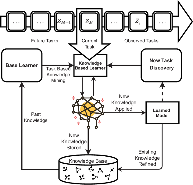
The lifelong learning algorithm diagram for our UAV-IoT system from the perspective of knowledge learning is presented in Fig. 2. Detailed procedures are as below:

1. 1.

   Initialize policy at devices: Random initialization policies are used at the very start.

2. 2.

   Collect trajectory: The UAV will randomly choose one device as its destination and flies to it. Upon arrival, it collects the trajectory from the device.

3. 3.

   New task discovery: The UAV uses the collected device trajectory to identify if it was experiencing a new environment since its last visit using the task discovery method described in Section II-B.

4. 4.

   Knowledge mining for current task: The task-specific knowledge contained in the Hessian matrix will be computed. Instead of looping until the policy parameters converge, only one run of the policy gradient update will be performed. The PG algorithm used to compute policy gradient will be called base learner.

5. 5.

   Refine knowledge base: If the identified task is new, the knowledge base will be refined according to (12) and (13). Otherwise, the outdated knowledge will be deducted before knowledge base refinement.

6. 6.

   Update model: The parameterized policy can be updated as in (9) and (10).

   

7. 7.

   Transmit updated policy back to the device: The updated policy for the current environment will be transmitted back to the device. The device will use it as the initial policy from now on before a new policy received from the UAV.

As such, the UAV can provide adaptive capabilities to the devices based on the accumulated knowledge. In the training phase, the knowledge base will be trained using 10 tasks distributed over 3 devices. During training, the same device will be visited by the UAV more than once. A new task will appear to a device only when the policy parameters of the previous task have converged. The training procedure ends when the policy parameters of all training tasks converge.

Finally, we show that our LLRL can support a variety of base learners. In theory, any policy based reinforcement learning algorithm that can provide an estimate of the Hessian matrix can be incorporated. Take REINFORCE [21] as an example. With Gaussian policy $\pi_{{\boldsymbol{\theta}}_{j}}(\boldsymbol{y}_{j,t}|\boldsymbol{x}_{j,t})\sim\mathcal{N}(\boldsymbol{\theta}_{j}^{\mathrm{T}}\boldsymbol{x}_{j},\boldsymbol{\sigma}_{j}^{2})$ considered, the first-order derivative has the following form: $-\mathbb{E}[\mathfrak{R_{j}}(\boldsymbol{\tau})(\sum_{t=0}^{T}\boldsymbol{\sigma}_{j}^{-2}\big(\boldsymbol{y}_{j,t}-\boldsymbol{\theta}_{j}^{\mathrm{T}}\boldsymbol{x}_{j,t}\big)\boldsymbol{x}_{j,t}^{\mathrm{T}})]$. Thus, the Hessian matrix can be easily obtained as: $\boldsymbol{\Gamma}_{j}=\mathbb{E}\Big[\sum_{t=0}^{T}\boldsymbol{\sigma}_{j}^{-2}\boldsymbol{x}_{j,t}\boldsymbol{x}_{j,t}^{\mathrm{T}}\Big]$.

References

- [1] A. Zanella, N. Bui, A. Castellani, L. Vangelista, and M. Zorzi, “Internet of things for smart cities,” IEEE Internet of Things Journal, vol. 1, no. 1, pp. 22–32, Feb 2014.
- [2] L. Da Xu, W. He, and S. Li, “Internet of things in industries: A survey,” IEEE Transactions on industrial informatics, vol. 10, no. 4, pp. 2233–2243, Jan. 2014.
- [3] S. Kaul, R. Yates, and M. Gruteser, “Real-time status: How often should one update?” in Proc. of IEEE International Conference on Computer Communications (INFOCOM), Orlando, FL, USA, March 2012.
- [4] B. Zhou and W. Saad, “Joint status sampling and updating for minimizing age of information in the internet of things,” IEEE Transactions on Communications, vol. 67, no. 11, pp. 7468–7482, July 2019.
- [5] X. Wu, J. Yang, and J. Wu, “Optimal status update for age of information minimization with an energy harvesting source,” IEEE Transactions on Green Communications and Networking, vol. 2, no. 1, pp. 193–204, Nov. 2017.
- [6] S. Kaul, M. Gruteser, V. Rai, and J. Kenney, “Minimizing age of information in vehicular networks,” in Proc. of 8th Annual IEEE Communications Society Conference on Sensor, Mesh and Ad Hoc Communications and Networks, Salt Lake City, UT, USA, June 2011.
- [7] Q. Wang, H. Chen, Y. Gu, Y. Li, and B. Vucetic, “Minimizing the age of information of cognitive radio-based IoT systems under a collision constraint,” arXiv preprint arXiv:2001.02482, 2020.
- [8] C. Chaccour and W. Saad, “On the ruin of age of information in augmented reality over wireless terahertz (THz) networks,” arXiv preprint arXiv:2008.09959, 2020.
- [9] R. Li, Q. Ma, J. Gong, Z. Zhou, and X. Chen, “Age of processing: Age-driven status sampling and processing offloading for edge computing-enabled real-time IoT applications,” arXiv preprint arXiv:2003.10916, 2020.
- [10] M. Mozaffari, A. T. Z. Kasgari, W. Saad, M. Bennis, and M. Debbah, “Beyond 5G with UAVs: Foundations of a 3D wireless cellular network,” IEEE Transactions on Wireless Communications, vol. 18, no. 1, pp. 357–372, Nov. 2018.
- [11] M. Chen, U. Challita, W. Saad, C. Yin, and M. Debbah, “Artificial neural networks-based machine learning for wireless networks: A tutorial,” IEEE Communications Surveys & Tutorials, vol. 21, no. 4, pp. 3039–3071, July 2019.
- [12] M. Chen, M. Mozaffari, W. Saad, C. Yin, M. Debbah, and C. S. Hong, “Caching in the sky: Proactive deployment of cache-enabled unmanned aerial vehicles for optimized quality-of-experience,” IEEE Journal on Selected Areas in Communications, vol. 35, no. 5, pp. 1046–1061, March 2017.
- [13] A. Ferdowsi, M. A. Abd-Elmagid, W. Saad, and H. S. Dhillon, “Neural combinatorial deep reinforcement learning for age-optimal joint trajectory and scheduling design in UAV-assisted networks,” IEEE Journal on Selected Areas in Communications (JSAC), Special Issue on Age of Information in Real-time Systems and Networks, 2021.
- [14] C. Xu, X. Wang, H. H. Yang, H. Sun, and T. Q. Quek, “AoI and energy consumption oriented dynamic status updating in caching enabled IoT networks,” arXiv preprint arXiv:2003.00383, 2020.
- [15] M. Hatami, M. Jahandideh, M. Leinonen, and M. Codreanu, “Age-aware status update control for energy harvesting IoT sensors via reinforcement learning,” arXiv preprint arXiv:2004.12684, 2020.
- [16] S. Thrun, “Lifelong learning algorithms,” in Learning to learn. Springer, 1998, pp. 181–209.
- [17] A. P. Chandrakasan, S. Sheng, and R. W. Brodersen, “Low-power cmos digital design,” IEICE Transactions on Electronics, vol. 75, no. 4, pp. 371–382, April 1992.
- [18] Z. Chen and B. Liu, “Lifelong machine learning,” Synthesis Lectures on Artificial Intelligence and Machine Learning, vol. 12, no. 3, pp. 1–207, Aug. 2018.
- [19] A. Kumar and H. Daume III, “Learning task grouping and overlap in multi-task learning,” arXiv preprint arXiv:1206.6417, 2012.
- [20] H. B. Ammar, E. Eaton, P. Ruvolo, and M. Taylor, “Online multi-task learning for policy gradient methods,” in Proc. of International Conference on Machine Learning, Beijing, China, June 2014.
- [21] R. J. Williams, “Simple statistical gradient-following algorithms for connectionist reinforcement learning,” Machine learning, vol. 8, no. 3-4, 1992.
- [22] J. L. Hill and D. E. Culler, “Mica: A wireless platform for deeply embedded networks,” IEEE micro, vol. 22, no. 6, pp. 12–24, 2002.