The first photometric investigation and spectroscopic analysis of two contact binaries: ASAS J124343+1531.7 and LINEAR 2323566
Abstract
The multi-color passband CCD light curves of ASAS J124343+1531.7 and LINEAR 2323566 were first obtained by the 0.84-m Ritchey-Chrétien telescope with follow up observations by the WIYN 0.90m Cassegrain telescope. The data from the of ASAS J124343+1531.7 was also applied for subsequent analysis. By analyzing the data through the W-D program, their mass ratios and fill-out factors were determined as 3.758, 1.438 and 31.8, 14.9, respectively. ASAS J124343+1531.7 is a W-subtype median contact binary, while LINEAR 2323566 is a W-subtype shallow contact binary, and the asymmetric light curves prove that they both have the O’Connell effect, which is generally explained by magnetic activity. The equivalent widths (EWs) of Hα lines were calculated, which show they certainly have magnetic activity. Moreover, LINEAR 2323566 has a stronger magnetic activity. The analysis of orbital period changes shows that ASAS J124343+1531.7 has a trend of secular period increase, which is generally explained by the mass transfer from the less massive to the more massive star. According to the estimated absolute parameters, their evolutionary states are discussed. The two components of ASAS J124343+1531.7 are both main sequence stars. While for LINEAR 2323566, the more massive star is a main sequence star, the less massive star has evolved out of main sequence and is over-luminous and over-sized.
Keywords:
binaries: close — binaries: eclipsing — binaries: spectroscopic — stars: individual: ASAS J124343+1531.7 and LINEAR 2323566I Introduction
W UMa type stars are close binary systems usually consisting of two late-type stars. The two stars fill or over-fill their Roche lobes, and there exists a common convective envelope(CCE) (Lucy 1968a; Lucy 1968b) around two components. Due to the existence of a CCE, there may be mass transfer and energy exchange between two components (Li et al. 2015; Liao et al. 2017; Lee & Park 2018; Li 2018, eg.,). The mass and angular momentum may also be lost from the binary system (Van‘t Veer 1979; Rahunen 1981; van Hamme 1982; Qian 2001a; Qian 2001b; Qian 2003, eg.,). Thus a series of physical processes will occur, such as the O’Connell effect (O’Connell 1951), thermal relaxation oscillation (TRO) (Lucy 1976; Flannery 1976; Robertson & Eggleton 1977, eg.,), orbital period change, short period cut-off etc (Ruciński 1992; Ruciński 2007; Stepień 2006; Jiang et al. 2012; Li et al. 2019, eg.,). In addition, there also exists the Applegate mechanism (Applegate 1992) and light-time effect (LTTE) (Irwin 1959; Mayer 1990; Wolf et al. 1999, eg.,), which can be used to explain the periodic changes of the orbital period of W UMa type stars. These physical characteristics make the contact binaries have a more complex evolutionary process. Accordingly, contact binaries are also of great significance for studying the formation and evolution of eclipsing binaries (Qian et al. 2017; Qian et al. 2018, eg.,)
ASAS J124343+1531.7 (2MASS J12434277+1531375, PY Com) was classified as an EW type binary star by Gettel et al. 2006 using the ROTSE-I telescope. Its period was reported as 0.266155 days, and the maximum and minimum V magnitude are 13.18 mag and 13.63 mag respectively. Later, Hoffman et al. 2009 defined ASAS J124343+1531.7 as a W UMa type star with a period of 0.30718 days. Drake et al. 2014 obtained the period for 0.26616 days and the amplitude of variation for 0.4 mag. Minimal timings of ASAS J124343+1531.7 were obtained by Diethelm 2009; Diethelm 2010; Diethelm 2011; Diethelm 2012. Nevertheless, the study of photometric solutions and the period variations have not been published yet. This paper presents the complete light curves first obtained in 2018, 2019 and 2020. Thereafter, the analyses of orbital period and photometric solutions were put forward.
LINEAR 2323566 (2MASS J11514615+4750292) was first observed by the asteroid survey LINEAR (Palaversa et al. 2013), it was identified as an eclipsing binary with a period of 0.232872 days. The median LINEAR magnitude and amplitude variation were determined as 15.24 mag and 0.8 mag respectively. Later, Drake et al. 2014 identified LINEAR 2323566 as an EW type binary star and determined a period of 0.23287 days by the Catalina Surveys Data Release-1 (CSDR1). It has no photometric analyses or period investigations. During our observations, two complete light curves were obtained in 2016 and 2020 to do the photometric solution. Due to the lack of minima from other literatures, we only analyzed the orbital period using our observation data.
II Observations
II.1 Photometric Observations
We observed ASAS J124343+1531.7 and LINEAR 2323566 using the 0.84-m f/15 Ritchey-Chrétien telescope at Observatorio Astronómico Nacional, Sierra San Pedro Mártir (OAN-SPM), Baja California, México, coupled with the Mexman filter-wheel and the Marconi3 CCD detector, equipped with Standard Johnson-Cousin-Bessel filters, in Feb., 2016, Apr., 2018 and Jan., 2019. As well as the WIYN 0.90m f/7.5 Cassegrain telescope at Kitt Peak National Observatory (KPNO), Arizona, USA, coupled with the Harris filter-wheel and the S2KB CCD detector followed up the observations in Feb. 2020. The log of observations is shown in Table 1. All these CCD images were reduced using the IRAF11 1 IRAF is distributed by the National Optical Astronomy Observatories, which are operated by the Association of Universities for Research in Astronomy under cooperative agreement with the National Science Foundation. package and has been corrected by bias and flat. In order to identify good comparison stars, and to determine the relative magnitudes of the variables, the field stars were calibrated during very photometric nights in which Landolt standard fields were also observed. Tables 2 and 3 list the HJD and the magnitudes of ASAS J124343+1531.7 and LINEAR 2323566. Figure 1 shows the light curves of the two objects in phase. The ephemeris used to convert time into phase is shown below,
| (1) |
where the is the primary minimum of light curve of each year. It can be seen from the light curves that both of them are W UMa type stars and show the O’Connell effect.
We also tried to find other sky survey data for these two targets, for example, All Sky Automated Survey (ASAS) (Paczynski et al. 2006), All-Sky Automated Survey for Supernovae (ASAS-SN) (Shappee et al. 2014), Catalina Sky Surveys (CSS) (Drake et al. 2014), TESS (Ricker et al. 2015), Northern Sky Variability Survey (NSVS) (Woźniak et al. 2004), etc. Although these two targets were both observed, the quality of survey data except TESS is not good enough to support subsequent analysis work. Finally, we adopted only the TESS data for ASAS J124343+1531.7. The TESS data processed by package (Lightkurve Collaboration et al. 2018) were downloaded from the Mikulski Archive for Space Telescopes (MAST)22 2 https://mast.stsci.edu/portal/Mashup/Clients/Mast/Portal.html. The time span is about 25 days from March 21, 2020 to April 15, 2020. In order to better show the overall light curve, we used Equation (1) to convert the BJD of TESS data into phase and obtained the complete light curves in one period plotted in Figure 2. Later, we also used this data for orbit period and photometric analysis.
| Objects | RA DEC | Date | Filter(Exposure Time [s]) | Filter(Number of data points) |
|---|---|---|---|---|
| ASAS J124343+1531.7 | 12 43 42.77 +15 31 37.46 | Apr. 22, 2018 | ||
| Jan. 24, 2019 | ||||
| Feb. 15, 2020 | ||||
| LINEAR 2323566 | 11 51 46.16 +47 50 29.45 | Mar. 20, 2016 | ||
| Feb. 16, 2020 |
| B | V | R | |||||
|---|---|---|---|---|---|---|---|
| HJD | M(mag) | HJD | M(mag) | HJD | M(mag) | ||
| April 22, 2018 | |||||||
| 2458230.69130 | 14.287 | 2458230.69072 | 13.417 | 2458230.69031 | 12.976 | ||
| 2458230.69337 | 14.316 | 2458230.69279 | 13.438 | 2458230.69238 | 13.004 | ||
| 2458230.69544 | 14.372 | 2458230.69486 | 13.469 | 2458230.69445 | 13.026 | ||
| 2458230.69751 | 14.403 | 2458230.69693 | 13.510 | 2458230.69652 | 13.058 | ||
| 2458230.69958 | 14.449 | 2458230.69900 | 13.561 | 2458230.69859 | 13.087 | ||
| … | … | … | … | … | … | ||
| 2458895.02813 | 14.260 | 2458895.02665 | 13.372 | 2458895.02518 | 12.934 | ||
| 2458895.03320 | 14.363 | 2458895.03136 | 13.433 | 2458895.02982 | 12.985 | ||
| 2458895.03834 | 14.462 | 2458895.03626 | 13.527 | 2458895.03471 | 13.070 | ||
| 2458895.04435 | 14.585 | 2458895.04208 | 13.621 | 2458895.04039 | 13.162 | ||
| 2458895.05094 | 14.583 | 2458895.04856 | 13.674 | 2458895.04703 | 13.232 | ||
| B | R | |||
|---|---|---|---|---|
| HJD | M(mag) | HJD | M(mag) | |
| March 20, 2016 | ||||
| 2457467.65545 | 16.732 | 2457467.65651 | 15.021 | |
| 2457467.65731 | 16.710 | 2457467.65943 | 15.020 | |
| 2457467.65835 | 16.706 | 2457467.66236 | 14.992 | |
| 2457467.66023 | 16.730 | 2457467.66528 | 14.979 | |
| 2457467.66127 | 16.683 | 2457467.66820 | 14.951 | |
| … | … | … | … | |
| 2458896.03358 | 17.004 | - | - | |
| 2458896.03710 | 17.104 | - | - | |
| 2458896.03902 | 17.128 | - | - | |
| 2458896.04271 | 17.221 | - | - | |
| 2458896.04459 | 17.307 | - | - | |


II.2 Spectroscopic Observations of LAMOST
Guoshoujing Telescope (the Large Sky Area Multi-Object Fiber Spectroscopic Telescope (LAMOST)) is a 4m reflecting Schmidt telescope equipped with 4000 fibers with a 5∘ field of view (Cui et al. 2012; Zhao et al. 2012). The wavelength coverage ranges from 3700 Å to 9000 Å (Du et al. 2016), and the overall spectral resolution of LAMOST is approximately 1800. The data were reduced with LAMOST pipelines (Luo et al. 2012). And the LAMOST spectral analysis pipeline (also called 1D pipeline, LASP) is used to classify and measure the spectra (Luo & Zhao 2001; Luo et al. 2004; Luo et al. 2008; Luo et al. 2012; Wang et al. 2010). Through LASP, the observed stellar spectra are classified into different subclasses by matching with template spectra (Wei et al. 2014). The spectra and parameters of ASAS J124343+1531.7 and LINEAR 2323566 were obtained from Data Release 733 3 http://dr7.lamost.org/ (Luo et al. 2015). Table 4 lists the spectral information of these two targets, including the observational data, Heliocentric Julian date, phase, spectral type, effective temperature (), , radial velocity (RV) and signal to noise ratio of r filter (SNR-r). We downloaded these spectra and plotted them in Figure 3.
| Targets | Obsdate | HJD(d) | Phase | Subclass | RV (km s-1) | SNR-r | EWs: Hα (Å) | ||
|---|---|---|---|---|---|---|---|---|---|
| ASAS J124343+1531.7 | Mar. 9, 2014 | 2456726.12748 | 0.11390 | G9 | 5221.7650.97 | 4.342 | -24.29 | 93.2 | 3.019 |
| Dec. 18, 2017 | 2458106.42784 | 0.05481 | G9 | 5083.8727.15 | 4.230 | -9.46 | 119.8 | 3.361 | |
| LINEAR 2323566 | Jan. 21, 2014 | 2456679.31742 | 0.39520 | K5 | 4464.3288.88 | 4.428 | 27.85 | 48.2 | 4.663 |


III Photometric Solutions
The 2015 version of the Wilson-Devinney (W-D) (Wilson & Devinney 1971; Wilson 1979; Wilson 1990; Wilson & van Hamme 2007) program was used to analyze the new multi-passband CCD photometry and obtained the model parameters. The effective temperatures used in the W-D program are from LAMOST listed in Table 4. Since ASAS J124343+1531.7 has two spectra, we assigned an average temperature of 5153153 K as the final effective temperature of the primary star. The effective temperature of the primary star used in calculation was 446489 K for LINEAR 2323566. According to Lucy 1967 and Ruciński 1969, the gravity-darkening coefficients and bolometric albedo coefficients were set as = 0.32 and = 0.5, respectively. Bolometric limb-darkening and bandpass limb-darkening coefficients were obtained from van Hamme 1993. The band is added to the limb-darkening table by Professor Van Hamme (private communication with Dr. Wang, Z. H.). During our modeling, Mode 3 was chosen for the two binary systems. Other parameters include the orbital inclination , the effective surface temperature of the secondary star , the dimensionless potentials of two components and the monochromatic luminosity of the primary star were set as adjustable parameters.
First, we used all the observed data from OAN-SPM, KPNO, and TESS for ASAS J124343+1531.7 and LINEAR 2323566 to do the -search process respectively, to determine their mass ratios. Then, we obtained solutions with mass ratios ranging from 0.1 to 10 with an interval of 0.1. The relationship between their mass ratios and residuals is shown in Figure 4. The mass ratios corresponding to their minimum residuals are 3.6 and 1.4, respectively. Consequently, we set them as the initial values of and adjustable, and thereafter, the convergent solutions for mass ratios 3.758 and 1.438 were obtained. The photometric solutions corresponding to these mass ratios are considered to be the final solution of these two objects, and are applied to determine the physical parameters and discuss the evolutionary status. All the parameters and errors of photometric solutions are listed in Table 5.
Since the two maxima of the light curves are not equal for these two objects, this indicates that they both exist O’Connell effect, which is generally caused by the existence of spots (Li et al. 2018, eg., V789 Her and V1007 Cas,). Therefore, we added spot parameters when using W-D program and fitted them according to observations at different times to study the changes of spots. We divide the data of ASAS J124343+1531.7 into three parts, 2018 & 2019, Feb., 2020 for our observations and Mar. & Apr., 2020 for TESS, while the data of LINEAR 2323566 into two parts, 2016 and 2020 for our observations. Their mass ratios are respectively set to 3.758 and 1.438, then the spot parameters are adjusted to obtain the best fitting solution. We have tried adding cool spot or hot spot on the primary or secondary stars, and finally we obtained the best results when we used a single cool spot on the hotter star. The theoretical light curves of different times are plotted in Figure 5, it can be seen that the two maxima of light curves fit well, the residuals between observed data and theoretical light curves are almost flat. The spot parameters at different times are listed in Table 6.
The geometric structure under different spot parameters at phase 0.25 and 0.75 are displayed in Figure 6, where the model of the binary systems and the location of the cool spot are displayed more intuitive. The dimension parameters of the corresponding geometric structure are also listed in Table 6. The errors obtained by the W-D method are mathematical fitting and have no physical meaning.
| Star | ASAS J124343+1531.7 | LINEAR 2323566 |
|---|---|---|
| 5153 | 4467 | |
| 3.758 0.028 | 1.438 0.040 | |
| 48335 | 438210 | |
| 77.40.2 | 87.4 0.6 | |
| 7.4040.037 | 4.348 0.063 | |
| 0.3350.003 | 0.465 0.003 | |
| 0.3140.003 | - | |
| 0.2990.003 | 0.449 0.003 | |
| 0.2900.001 | - | |
| 0.287 0.001 | 0.3580.003 | |
| 0.515 0.004 | 0.4230.013 | |
| 31.8 5.8 % | 14.910.9 % |


![[Uncaptioned image]](2103.15322v1/wd_LINEAR2323566_1.png)
![[Uncaptioned image]](2103.15322v1/wd_LINEAR2323566_2.png)
Fig. 5 - Continued
| Star | ASAS J124343+1531.7 | LINEAR 2323566 | |||
|---|---|---|---|---|---|
| Year | 2018 & 2019 | Feb., 2020 | Mar. & Apr., 2020 | 2016 | 2020 |
| Spot | Star 1 | Star 1 | Star 1 | Star 1 | Star 1 |
| 86.9 9.1 | 105 8 | 102 2 | 101 27 | 103 14 | |
| 275.3 4.1 | 275 14 | 257 2 | 269 3 | 249 4 | |
| 17.0 0.5 | 16 1 | 17 1 | 17 0 | 19 1 | |
| 0.71 0.03 | 0.71 0.08 | 0.71 0.01 | 0.73 0.03 | 0.72 0.05 | |
| 0.261 | 0.258 | 0.267 | 0.338 | 0.334 | |
| 0.273 | 0.270 | 0.280 | 0.355 | 0.351 | |
| 0.314 | 0.307 | 0.327 | 0.394 | 0.388 | |
| 0.474 | 0.471 | 0.479 | 0.398 | 0.394 | |
| 0.513 | 0.509 | 0.521 | 0.423 | 0.418 | |
| 0.541 | 0.536 | 0.550 | 0.457 | 0.451 | |

![[Uncaptioned image]](2103.15322v1/structure2.png)
Fig. 6 - Continued
IV Orbital Period Analysis
In order to analyze the orbital period changes of ASAS J124343+1531.7 and LINEAR 2323566, we used the K-W method (Kwee & van Woerden 1956) to calculate the eclipsing times. However, the time resolution of TESS data for ASAS J124343+1531.7 is low, on account of the 30 minute observation cadence. Therefore, we used the phase shift method to apply higher density light curves. First, we divided TESS light curves into four parts, the BJD time span of these four parts are 2458929.51622 to 2458935.24541, 2458936.26624 to 2458940.82870, 2458946.74526 to 2458951.32849 and 2458951.34932 to 2458954.80755, and the number of points in each part is 234, 215, 165 and 166, respectively. Second, using the equation BJD = BJD0 + P E, where BJD is the observing time, BJD0 is the reference time for each part, which are 2458932.120404, 2458938.245397, 2458948.620222 and 2458952.620118, and P is the orbital period of ASAS J124343+1531.7. Ultimately, we moved the long time-span data into one period and determined the four panels of Figure 8. Then, we obtained 8 eclipsing times from these four sets of light curves.
Combining other literatures, public data and our own observations, we have collected 16 and 4 minima for ASAS J124343+1531.7 and LINEAR 2323566 respectively shown in Table 7. The ephemerides used to calculate (observation-calculation) values are:
| (2) |
Since the minimum moments of TESS data for ASAS J124343+1531.7 are given in BJD, we converted other observed minima from HJD to BJD. The calculated epoch and values were also listed in Table 7, and the corresponding data points were plotted in Figure 8.
The trend of ASAS J124343+1531.7 shows slightly nonlinear variations. Therefore we fitted the values with an upward parabola, where the revised ephemeris is as follows,
| (3) |
From Equation (3), the coefficients of second-order term are positive, indicating that the period of ASAS J124343+1531.7 is secular increase and the rate is calculated as = 1.239 10-7 . After removing the parabolic term from trend, the residuals are plotted in the lower panel. The residuals are almost flat, which indicates the values were fitted well. While LINEAR 2323566 has very few data points, and the distribution of data points shows no nonlinear change, as shown on Figure 8. Therefore, we only performed simple linear fitting on LINEAR 2323566, and obtained the new ephemeris as follows,
| (4) |
The residuals of the fitting are also displayed in the bottom panel of Figure 8, and the corresponding data are listed in Table 7.
Due to the 2015 version of the W-D program can also analyze the times of minima, then we included the minima data of these two objects during the W-D process to solve the epoch, period and orbital period variation. Then, we transformed the results into the form of Equations (3) and (4) as shown below,
| (5) |
| (6) |
Equation (5) is for ASAS J124343+1531.7, which exists a long-term increase in the orbital period, and the rate is calculated as = 1.241 10-7 . Equation (6) is for LINEAR 2323566, which obtained a new linear ephemeris. By comparison, it can be seen that the results of the two methods are almost the same.


| JD (Barycentric)2400000+ | Error | Type | Min. | Epoch | Res. | References | |
|---|---|---|---|---|---|---|---|
| ASAS J124343+1531.7 | |||||||
| 54955.7337 | 0.0011 | ccd | s | -12304.5 | 0.0123 | -0.0002 | (1) |
| 55280.7162 | 0.0003 | ccd | s | -11083.5 | 0.0110 | 0.0004 | (2) |
| 55616.8773 | 0.0006 | ccd | s | -9820.5 | 0.0095 | 0.0007 | (3) |
| 55983.9104 | 0.0006 | ccd | s | -8441.5 | 0.0052 | -0.0018 | (4) |
| 56050.7191 | 0.0021 | ccd | s | -8190.5 | 0.0072 | 0.0006 | (4) |
| 58230.7117 | 0.0002 | ccd | p | 0.0 | 0.0000 | 0.0003 | (5) |
| 58508.0525 | 0.0002 | ccd | p | 1042.0 | 0.0000 | 0.0007 | (5) |
| 58894.9169 | 0.0003 | ccd | s | 2495.5 | -0.0021 | -0.0009 | (5) |
| 58932.1801 | 0.0002 | ccd | s | 2635.5 | -0.0015 | -0.0003 | (6) |
| 58932.3137 | 0.0002 | ccd | p | 2636.0 | -0.0011 | 0.0002 | (6) |
| 58938.3020 | 0.0001 | ccd | s | 2658.5 | -0.0014 | -0.0001 | (6) |
| 58938.4355 | 0.0001 | ccd | p | 2659.0 | -0.0010 | 0.0003 | (6) |
| 58948.6821 | 0.0001 | ccd | s | 2697.5 | -0.0017 | -0.0004 | (6) |
| 58948.8160 | 0.0001 | ccd | p | 2698.0 | -0.0008 | 0.0004 | (6) |
| 58952.6745 | 0.0001 | ccd | s | 2712.5 | -0.0017 | -0.0004 | (6) |
| 58952.8084 | 0.0001 | ccd | p | 2713.0 | -0.0008 | 0.0005 | (6) |
| LINEAR 2323566 | |||||||
| 57467.7355 | 0.0002 | ccd | p | 0.0 | 0.0000 | 0.0002 | (5) |
| 57467.8515 | 0.0001 | ccd | s | 0.5 | -0.0004 | -0.0002 | (5) |
| 57467.9683 | 0.0002 | ccd | p | 1.0 | -0.0001 | 0.0001 | (5) |
| 58895.9397 | 0.0003 | ccd | p | 6133.0 | -0.0084 | 0.0000 | (5) |
Ref. (1) Diethelm 2009; (2) Diethelm 2010; (3) Diethelm 2011; (4) Diethelm 2012; (5) This paper; (6) TESS


V Spectral analyses
Since both ASAS J124343+1531.7 and LINEAR 2323566 exhibit the O’Connell effect, we used a spot generally caused by magnetic activity to explain this phenomenon. In order to further confirm whether in these two objects exist magnetic activity, we analyzed the spectral lines below. The observed spectra not only shows chromospheric activity, but also mix in some spectral lines of photosphere. In order to use the intensity of Hα line to analyze their magnetic activity, we adopted a spectral subtraction technique conducted by Barden 1985. Some other objects also used this method, for example, ASAS J082243+1927.0 (Kandulapati et al. 2015), EPIC 202073314 (Sriram et al. 2018), V582 Lyr (Cheng et al. 2019); V384 Ser, AQ Psc, V480 Gem and 2MASS J07095549+3643564 (Zhang et al. 2020).
First, we selected some targets with a temperature difference of 100K above or below our objects from a catalogue of radial velocity standard stars (Huang et al. 2018). Then we used these targets to search in LAMOST Data Release 7. Finally, we obtained 7 and 8 template spectra for ASAS J124343+1531.7 and LINEAR 2323566, respectively, and used these inactive spectra to construct the synthesized spectra. Combining the object and template spectra, a total of 18 spectra were normalized by IRAF package Continuum. We obtained their residuals by subtracting the comprehensive spectra from the object spectra, and all the spectra exclude the region of Hα. Then the best template spectra were determined as 2MASS J19141861+4238492 and KIC 7446560 for the two objects respectively. The spectral type and temperature were determined as K1 and 5028K for 2MASS J19141861+4238492, K5 and 4377K for KIC 7446560. We subtracted their best template spectra from the observed spectra to obtain the subtracted spectra, which is the chromospheric construction. All of the observed, synthesized and subtracted spectra are displayed in Figure 9. From the intensity of emission line Hα, LINEAR 2323566 has stronger chromospheric activity than ASAS J124343+1531.7. The equivalent widths (EWs) were calculated using IRAF package Splot, which are listed in Table 4.


VI Discussions and Conclusions
Using the light curve analysis, we determined the physical parameters of ASAS J124343+1531.7 and LINEAR 2323566, which are shown in Table 5. The mass ratio and fill-out factor are 3.758 0.028 and 31.8 5.8 for ASAS J124343+1531.7, 1.438 0.040 and 14.9 10.9 for LINEAR 2323566. Therefore, ASAS J124343+1531.7 is a W-subtype median contact binary, while LINEAR 2323566 is a W-subtype shallow contact binary. The O’Connell effect of these two systems prove that it may exist magnetic activity. Spectral analysis obtained the EWs of the emission line Hα, which confirmed the possibility of magnetic activity of these two objects.
According to Yakut & Eggleton 2005, the statistics show that the more massive stars of W-type and A-type low-temperature contact binaries (LTCBs) usually locate in the main sequence. Consequently, assuming the more massive star is a main sequence star and referring to Cox 2000, the spectral type of the more massive star is classified by the effective temperature as K3 and K5, then the mass was determined by the spectral type as = 0.75, 0.68. Subsequently the mass of less massive star is also calculated according to the mass ratio and the mass of more massive star, = 0.20, 0.47. Combining the mass and period, the orbital semi-major axis was determined using the third law of Kepler, , = 1.71, 1.67. Simultaneously, the radius and luminosity of the two components were computed by using the photometric solutions and Stefan-Boltzman law, = 0.49, 0.60, = 0.88, 0.71, = 0.15, 0.13, = 0.38, 0.17. The error bars are obtained by error transmission. All the absolute parameters of ASAS J124343+1531.7 and LINEAR 2323566 are listed in Table 8.
Both of the two targets have been observed by Gaia (Gaia Collaboration et al. 2016; Gaia Collaboration et al. 2018), we obtained the Gaia distances, 361.8 pc for ASAS J124343+1531.7 and 678.7 pc for LINEAR 2323566. Considering the interstellar extinction, we calculated their apparent magnitudes using luminosity from WD solution and Gaia distance, and obtained 13.536 mag for ASAS J124343+1531.7 and 15.838 mag for LINEAR 2323566. Our apparent magnitude of photometric values is about 13.20 mag for ASAS J124343+1531.7, while apparent magnitude from Drake et al. 2014 is 15.38 mag for LINEAR 2323566. The apparent magnitudes derived by the two methods are somewhat different, this may be caused by that there are some differences between the estimated absolute parameters and the real ones.
| ASAS J124343+1531.7 | LINEAR 2323566 | |||
|---|---|---|---|---|
| Components | Primary | Secondary | Primary | Secondary |
| Mass () | 0.200.01 | 0.750.02 | 0.470.03 | 0.680.02 |
| Radius () | 0.490.01 | 0.880.01 | 0.600.01 | 0.710.03 |
| Luminosity () | 0.150.02 | 0.380.06 | 0.130.02 | 0.170.03 |
| Semi-major axis () | 1.710.01 | 1.670.03 | ||
VI.1 Mass transfer between two components
According to the analysis of the orbital period, the overall trend of shows an upward parabolic composition with a rate of = 1.239 10-7 for ASAS J124343+1531.7. The long-term increase can probably be explained by the mass transfer from the less massive to the more massive star. Then we used the following equation to calculate the rate of mass transfer,
| (7) |
yr-1 was determined. The negative sign indicates that the less massive star is losing mass, while the more massive star is receiving mass. Then we discuss the possible subsequent evolution of ASAS J124343+1531.7. As the mass transfer, mass ratio will increase and the distance between the two components will increase. Therefore, the degree of contact will gradually become smaller, ASAS J124343+1531.7 will evolve from the current contact binary to a semi-contact binary or detached binary. Consequently, ASAS J124343+1531.7 is a good target for studying the thermal relaxation oscillation (TRO) model (Lucy 1976; Flannery 1976; Robertson & Eggleton 1977), follow-up observations are also needed to confirm this result.
VI.2 Evolutionary status
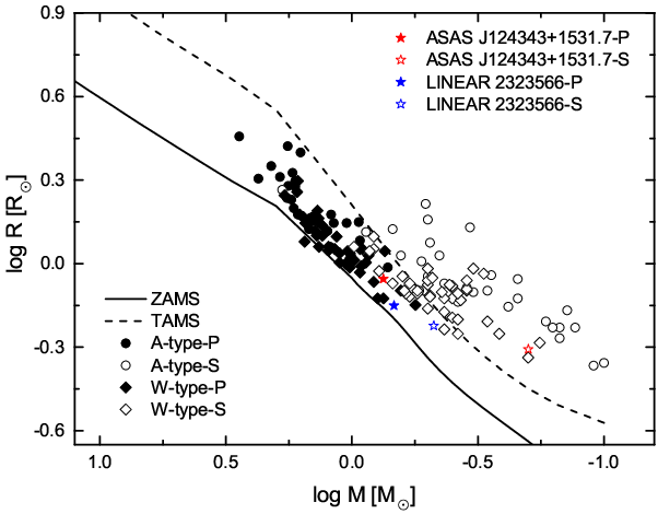
In order to study the evolutionary status of these two objects, the diagram of mass-luminosity and mass-radius were plotted in Figure 10. The solid and dotted lines show the zero age main sequence (ZAMS) and the terminal age main sequence (TAMS) constructed by the BSE Code (Hurley et al. 2002). Circles and rhombuses respectively represent 30 A-subtype and 42 W-subtype binary derived from Yakut & Eggleton 2005. Red stars and blue stars respectively represent the two components of ASAS J124343+1531.7 and LINEAR 2323566. All solid symbols represent the more massive components, whereas the open symbols denote the less massive ones. The positions of the two objects in the diagram are consistent with the trend of the other binaries. The more massive stars of ASAS J124343+1531.7 and LINEAR 2323566 locate above the ZAMS line and below the TAMS line. The less massive star of ASAS J124343+1531.7 locates above the TAMS line, while LINEAR 323566 locates above the ZAMS line and below the TAMS line. This manifests that the two components of LINEAR 2323566 are both slightly evolved stars. And for ASAS J124343+1531.7, the more massive star is a main sequence star, the less massive star has evolved out of the main sequence and is over-luminous and over-sized.
In summary, the photometric solutions and period variation of ASAS J124343+1531.7 and LINEAR 2323566 were obtained first. Through light curve analysis, it is found that ASAS J124343+1531.7 is a W-subtype median contact binary, while LINEAR 2323566 is a W-subtype shallow contact binary. They both present the O’Connell effect, which can be explained by a cool spot on the primary star. The existence of the cool spot may be caused by magnetic activity, and at the same time, the weak H emission lines on the spectra also indicate that the two objects possess magnetic activity. Through the analysis of the orbital period, we obtained ASAS J124343+1531.7 exists a secular period increase, which is likely caused by the mass transfer from the less massive star to the more massive star. We obtained a new ephemeris for LINEAR 2323566. The two components of ASAS J124343+1531.7 are both main sequence stars. While for LINEAR 2323566, the more massive star is a main sequence star, the less massive star has evolved out of main sequence and is over-luminous and over-sized. In the future, more observations combining photometry and spectra are needed to verify the variations of orbital period and the evolution of ASAS J124343+1531.7 and LINEAR 2323566.

References
- Applegate (1992) Applegate, J. H. 1992, ApJ, 385, 621
- Barden (1985) Barden, S. C., 1985, ApJ, 295, 162
- Cui et al. (2012) Cui, X.-Q., Zhan, Y.-H., Chu, Y.-Q., et al. 2012, RAA, 12, 1197
- Cheng et al. (2019) Cheng, Y., Zhang, L.-Y., Han, X. L., et al. 2019, AJ, 158, 193
- Cox (2000) Cox, A. N. 2000, Allens Astrophysical Quantities (4th ed.; New York: Springer)
- Diethelm (2009) Diethelm, R. 2009, IBVS, 5894, 1
- Diethelm (2010) Diethelm, R. 2010, IBVS, 5945, 1
- Diethelm (2011) Diethelm, R. 2011, IBVS, 5960, 1
- Diethelm (2012) Diethelm, R. 2012, IBVS, 6029, 1
- Drake et al. (2014) Drake, A. J., Graham, M. J., Djorgovski, S. G., et al. 2014, ApJS, 213, 9
- Du et al. (2016) Du, B., Luo, A.-L., Kong, X., et al. 2016, ApJS, 227, 27
- Flannery (1976) Flannery, B.P. 1976, ApJ, 205, 217
- Gaia Collaboration et al. (2016) Gaia Collaboration, Prusti, T., de Bruijne, J. H. J. et al. 2016, A&A, 595, 1
- Gaia Collaboration et al. (2018) Gaia Collaboration, Brown, A. G. A., Vallenari, A. et al. 2018, A&A, 616, 1
- Gettel et al. (2006) Gettel, S. J., Geske, M. T., & McKay, T. A. 2006, AJ, 131, 621
- Hoffman et al. (2009) Hoffman, D. I., Harrison, T. E., & McNamara, B. J. 2009, AJ, 138, 466
- Huang et al. (2018) Huang, Y., Liu, X. -W., Chen, B. -Q., et al. 2018, 156, 90
- Hurley et al. (2002) Hurley, J. R., Tout, C. A., & Pols, O. R. 2002, MNRAS, 329, 897
- Irwin (1959) Irwin J. B. 1959, AJ, 64, 149
- Jiang et al. (2012) Jiang, D., Han, Z., Ge, H., et al. 2012, MNRAS, 421, 2769
- Kandulapati et al. (2015) Kandulapati, S., Devarapalli, S. P., & Pasagada, V. R. 2015, MNRAS, 446, 510
- Kwee & van Woerden (1956) Kwee, K. K., & van Woerden, H. 1956, BAN, 12, 327
- Lee & Park (2018) Lee, J. W., & Park, J.-H., 2018, PASP, 130, 4201
- Li et al. (2015) Li, K., Hu, S.-M., Guo, D.-F., et al. 2015, AJ, 149, 120
- Li (2018) Li, K., 2018, NewA, 59, 60
- Li et al. (2018) Li, K., Xia, Q.-Q., Hu, S.-M., et al. 2018, PASP, 130, 4201
- Li et al. (2019) Li, K., Xia, Q.-Q., Michel, R., et al. 2019, MNRAS, 485, 4588
- Liao et al. (2017) Liao, W.-P., Qian, S.-B., Soonthornthum, B., et al. 2017, PASP, 129, 4204
- Lightkurve Collaboration et al. (2018) Lightkurve Collaboration, Cardoso, J. V. d. M., Hedges, C., et al. 2018, ascl.soft, 1812.013
- Lucy (1968a) Lucy, L. B., 1968a, ApJ, 151, 877
- Lucy (1968b) Lucy, L. B., 1968b, ApJ, 153, 1123
- Lucy (1967) Lucy, L. B. 1967, Z. Astrophys., 65, 89
- Lucy (1976) Lucy, L. B., 1976, ApJ, 205, 208
- Luo & Zhao (2001) Luo, A.-L., & Zhao, Y.-H. 2001, ChJAA, 1, 563
- Luo et al. (2004) Luo, A.-L., Zhang, Y.-X., & Zhao, Y.-H. 2004, Proc.SPIE, 5496, 756
- Luo et al. (2008) Luo, A.-L., Wu, Y., Zhao, J., & Zhao, G. 2008, Proc. SPIE, 7019, 701935
- Luo et al. (2012) Luo, A.-L., Zhang, H.-T., Zhao, Y.-H., et al. 2012, RAA, 12, 1243
- Luo et al. (2015) Luo, A.-L., Zhao, Y.-H., Zhao, G., et al. 2015, RAA, 15, 1095
- Mayer (1990) Mayer P., 1990, Bull. Astron. Inst. Czechoslovakia, 41, 231
- O’Connell (1951) O’Connell, D. J. K. 1951, MNRAS, 111, 642
- Paczynski et al. (2006) Paczynski, B., Szczygiel, D., Pilecki, B., et al. 2006, MNRAS, 368, 1311
- Palaversa et al. (2013) Palaversa, L., Ivezić, Ž., Eyer, L., et al. 2013, AJ, 146, 101
- Qian (2001a) Qian, S.-B. 2001a, MNRAS, 328, 635
- Qian (2001b) Qian, S.-B. 2001b, MNRAS, 328, 914
- Qian (2003) Qian, S.-B. 2003, MNRAS, 342, 1260
- Qian et al. (2017) Qian, S.-B., He, J.-J., Zhang, J., et al. 2017, RAA, 17, 87
- Qian et al. (2018) Qian, S.-B., Zhang, J., He, J.-J., et al. 2018, ApJS, 235, 5
- Rahunen (1981) Rahunen, T. 1981, A&A 102, 81
- Ricker et al. (2015) Ricker G. R., et al. 2015, J. Astron. Telesc. Inst. Syst., 1, 014003
- Robertson & Eggleton (1977) Robertson, J. A. & Eggleton, P. P. 1977, MNRAS, 179, 359
- Ruciński (1969) Ruciński, S. M. 1969, Acta Astron., 19, 245
- Ruciński (1992) Ruciński, S. M. 1992, AJ, 103, 960
- Ruciński (2007) Ruciński, S. M. 2007, MNRAS, 382, 393
- Stepień (2006) Stepień, K. 2006, AcA, 56, 347
- Shappee et al. (2014) Shappee, B. J., Prieto, J. L., Grupe, D., et al. 2014, ApJ, 788, 48
- Sriram et al. (2018) Sriram, K., Malu, S., Choi, C. S., et al. 2018, AJ, 155, 172
- Van‘t Veer (1979) Van‘t Veer F. 1979, A&A, 80, 287
- van Hamme (1982) van Hamme, W. 1982, A&A, 105, 389
- van Hamme (1993) van Hamme, W. 1993, AJ, 106, 2096
- Wang et al. (2010) Wang, F., Luo, A., & Zhao, Y. 2010, Proc. SPIE, 7740, 310
- Wei et al. (2014) Wei, P., Luo, A.-L,, Li, Y.-B., et al. 2014, 147, 101
- Wilson & Devinney (1971) Wilson, R. E., & Devinney, E. J. 1971, ApJ, 166, 605
- Wilson (1979) Wilson, R. E. 1979, ApJ, 234, 1054
- Wilson (1990) Wilson, R. E. 1990, ApJ, 356, 613
- Wilson & van Hamme (2007) Wilson, R. E., & van Hamme, W. 2007, Astronomy Department, University of Florida, Gainesville
- Wolf et al. (1999) Wolf, M., Diethelm, R., & Šarounová, L. 1999, A&A, 345, 553
- Woźniak et al. (2004) Woźniak, P. R., Vestrand, W. T., Akerlof, C. W., et al. 2004, AJ, 127, 2436
- Yakut & Eggleton (2005) Yakut, K., & Eggleton, P. P. 2005, ApJ, 629, 1055
- Zhao et al. (2012) Zhao, G., Zhao, Y.-H., Chu, Y.-Q., et al. 2012, RAA, 12, 723
- Zhang et al. (2020) Zhang, L. Y., Zhu, Z. Z., Yue, Q., et al. 2020, MNRAS, 491, 6065