On the linear stability of -boson stars with respect to radial perturbations
Abstract
In previous work we constructed new boson star solutions consisting of a family of massive complex scalar fields minimally coupled to gravity in which the individual fields have angular momentum, yet the configuration as a whole is static and spherically symmetric. In the present article we study the linear stability of these -boson stars with respect to time-dependent, radial perturbations. The pulsation equations, governing the dynamics of such perturbations are derived, generalizing previous work initiated by M. Gleiser, and shown to give rise to a two-channel Schrödinger operator. Using standard tools from the literature, we show that for each fixed value of the angular momentum number, there exists a family of -boson stars which are linearly stable with respect to radial fluctuations; in this case the perturbations oscillate in time with given characteristic frequencies which are computed and compared with the results from a nonlinear numerical simulation. Further, there is also a family of -boson stars which are linearly unstable. The two families are separated by the configuration with maximum mass. These results are qualitatively similar to the corresponding stability results of the standard boson stars with , and they imply the existence of new stable configurations that are more massive and compact than usual boson stars.
pacs
04.20.-q, 04.25.Dm, 95.30.Sf, 98.80.JkI Introduction
A boson star Kaup 1968; Ruffini and Bonazzola 1969; Jetzer 1992; Schunck and Mielke 2003; Liebling and Palenzuela 2012 is a hypothetical object described by a classical solution to the stationary Einstein-Klein-Gordon (EKG) system which is sourced by a complex, massive scalar field whose time-dependency is harmonic. In their most simple realization boson stars are static and spherically symmetric, although rotating generalizations which are stationary and axisymmetric have also been found long time ago Schunck and Mielke 1996; Yoshida and Eriguchi 1997. Beyond their simplicity, it has recently been shown using numerical evolutions of the fully nonlinear dynamical equations that static and spherically symmetric boson stars also naturally arise as the final state of binary boson star collisions, while rotating boson stars have not been observed to form in such a process Palenzuela et al. 2017. This is due to gravitational cooling Seidel and Suen 1994; Sanchis-Gual et al. 2019, which radiates all the angular momentum of the system.
In a previous paper Alcubierre et al. 2018 we showed that boson stars, as they were originally introduced in the late sixties, do not constitute the most general solution to the static spherically symmetric EKG system. Standard boson stars can be easily generalized if the internal symmetry group is extended from to with arbitrary odd values of . In this way, the internal group can hide not only the time dependency of the field but also the angular dependency of nontrivial harmonics if their amplitudes are excited in an appropriate way Olabarrieta et al. 2007. We dubbed these new states -boson stars in Alcubierre et al. 2018, with an arbitrary nonnegative integer.
Astrophysical realizations of -boson stars demand such configurations to be dynamically stable. Thus, the study of their stability is of utmost importance. Previous stability studies of boson stars, which correspond to the particular case of -boson stars with and , have been performed based on different approaches. Early studies focused on semi-analytic methods based on linear perturbation theory Gleiser 1988; Gleiser and Watkins 1989; T. D. Lee 1989 in which the EKG system is truncated at linear order. Later, these studies were complemented with nonlinear stability analyses evolving the full EKG equations with the help of numerical codes Balakrishna et al. 1998; Seidel and Suen 1990; Hawley and Choptuik 2000; Guzman 2009 (see also Kusmartsev et al. 1991 for an analysis based on catastrophe theory). The results of both types of approaches show that static, spherically symmetric -boson stars with possess both stable and unstable branches in the solution space, similar to what occurs in spherical relativistic fluid stars Chandrasekhar 1964a; Chandrasekhar 1964b; Shapiro and Teukolsky 1983.
-boson stars have scalar fields, and in principle each of these fields can be perturbed in an independent way. However, a simplification occurs if one assumes that the fields are described by the same radial perturbation, in which case spherical symmetry is preserved at the level of the perturbed configurations. Based on this assumption, in recent work Alcubierre et al. 2019 we have performed full nonlinear numerical simulations of the spherical EKG system. Our study indicates that -boson stars have similar stability properties than the standard stars, namely the -boson stars possess both stable and unstable branches of solutions. Moreover, it was found in Alcubierre et al. 2019 that small perturbations of stable configurations may exhibit extremely long-lived oscillations. The main purpose of the present work is to perform a linear stability analysis of -boson stars, based on the aforementioned assumption of spherical symmetry, and prove that there is, indeed, a stable branch which is characterized by the absence of growing modes and the presence of oscillatory modes in the spherically symmetric sector.
Regarding the stability of -boson stars with respect to nonspherical perturbations, recent numerical evolutions of the full 3D EKG equations indicate that within the timescales explored, the configurations belonging to the spherical stable branch do not possess nonspherical growing modes Jaramillo et al. 2020. In a recent work, Sanchis-Gual, et.al. Sanchis-Gual et al. 2021 have provided numerical evidence that -boson stars are in fact symmetry-enhanced stable points of larger continuous families of multi-field, multi-frequency boson stars. Although it would be desirable to confirm these findings through a semi-analytic linear stability analysis including nonspherical modes, such a study lies beyond the scope of the present work. Therefore, as mentioned previously, here we restrict ourselves to spherical linear perturbations.
This work is organized as follows. We start in section II with a brief review on the spherically symmetric field equations and conserved quantities which are relevant for this work and provide a short description of the main behavior of the equilibrium configurations constructed in Alcubierre et al. 2018. Next, in section III we derive the pulsation equations, describing the dynamics of linearized radial perturbations of the -boson star ground state configurations, generalizing previous work by Gleiser Gleiser 1988 and by Gleiser and Watkins Gleiser and Watkins 1989. These equations have the form of a coupled wave system with matrix-valued potential, and for modes with a harmonic time dependency they give rise to a self-adjoint coupled system of radial Schrödinger equations. We discuss various properties of the corresponding Schrödinger operator, including the asymptotic behavior of the mode solutions near the center and at infinity and the generalized nodal theorem proven in Amann and Quittner 1995, which allows one to determine the number of bound states with negative energy (corresponding to unstable exponentially in time growing modes in our system) by counting the number of zeros of a certain determinant. In Section IV we present the main results of this paper, starting with a computation for the number of negative energy bound states for different -boson star configurations. These results show that, as expected from the numerical simulations in our accompanying paper Alcubierre et al. 2019, the configurations on the stable branch are linearly stable, while the configurations lying on the unstable branch are linearly unstable. Next, based on a shooting algorithm for determining the ground state energy of the Schrödinger operator, we compute the oscillation frequencies of the perturbations for the stable configurations, and compare them to the frequencies found in the numerical simulations performed in Alcubierre et al. 2019. Conclusions are drawn in section V and technical details used in the numerical integration and shooting algorithm are included in an appendix at the end of the article.
Throughout this work, we use the signature convention for the spacetime metric and Planck units such that . As in our previous articles Alcubierre et al. 2018; Alcubierre et al. 2019, for simplicity, we restrict our attention to the case in which the scalar field is minimally coupled to gravity and is not self-interacting.
II Spherically symmetric field equations and equilibrium configurations
In this section we review briefly the construction leading to the -boson stars Alcubierre et al. 2018. These configurations give rise to a new class of static, spherically symmetric solutions of the EKG system, where the internal global symmetry of the standard boson star model is promoted to an arbitrary group. Accordingly, the scalar field consists of components, that for convenience can be seen as a collection of complex scalar fields , , of equal mass that we choose without self-interaction and minimally coupled to gravity. The spacetime metric describing these solutions (and their time-dependent generalizations) is parametrized in terms of the Misner-Sharp mass and the lapse functions according to
| (1) |
where is the areal radial coordinate and denotes the standard line element on the unit two-sphere. The most simple realization of a nontrivial -boson star appears for an odd different from one, with the components of the scalar field given by
| (2) |
Notice that the total angular momentum number is given in terms of a fixed nonnegative integer, and takes values , for a total of components. As usual denotes the standard spherical harmonics normalized such that , and the field amplitude is the same for all . As shown in Alcubierre et al. 2018 (see also Olabarrieta et al. 2007), this leads to a total stress energy-momentum tensor11 1 Notice that in this paper we follow the same conventions as in reference Alcubierre et al. 2018 regarding the normalization of the scalar field; hence relative to reference Alcubierre et al. 2019 the normalization of the stress energy-momentum tensor, equation (3), and the conserved current, equation (7), differs by a factor of .
| (3) |
( denoting the complex conjugate of ) which is spherically symmetric. If the symmetry group is large enough, different values of could be excited at the same time in the configuration; however, for the purposes of this paper we restrict our attention to the case with only one .
With the ansätze described in equations (1,2), the EKG system reduces to the following system of equations Alcubierre et al. 2018:
| (4a) | |||||
| (4b) | |||||
| (4c) | |||||
| (4d) | |||||
| (4e) | |||||
with and where and . Here and in the following, a dot and a prime denote partial derivatives with respect to and , respectively.
The -boson star solutions described in Alcubierre et al. 2018 are obtained by integrating these equations for the time-harmonic ansatz
| (5) |
with a real frequency and a real-valued function of , which behaves as in the vicinity of the center and decays exponentially fast as . In this way one finds, numerically and for each , families of solutions which can be parametrized by and the number of nodes of the function inside the interval . In this work we restrict our attention to ground state solutions, for which has no nodes. Similar to the case of the standard boson stars with , as the value of increases from zero, the total mass
| (6) |
of the configurations (which coincides with the Arnowitt-Deser-Misner mass) starts increasing, but at some point develops a maximum after which it decreases, see the left panel of figure 1 for details. The numerical simulations performed in Alcubierre et al. 2019 indicate that the configurations belonging to values of below the one corresponding to the maximum of the mass are stable with respect to small (but nonlinear) spherical perturbations, while the configurations with larger are unstable, and either collapse to a black hole, or (depending on the sign of the binding energy) migrate to a stable configuration or disperse to infinity. Thus the behavior is analogous to the standard boson star solutions in which the maximum mass configuration divides the solution curve into “stable” and “unstable” branches. Similarly, the compacticity, defined as , where is the radius of a sphere containing 99% of the total mass, starts increasing as increases, until it develops a maximum. However, note that this maximum occurs at a higher value of than the one corresponding to the maximum mass configuration, see the right panel of figure 1. As we can appreciate from this figure, larger values of allow not only for more massive (stable) solutions, but also for larger compacticities. That is, there exist stable solutions that can be more compact than the standard boson stars. Furthermore, the larger the value of , the more compact the stable solutions can be, at least for the first values of the angular momentum number that we have explored in this paper. As mentioned in the introduction, the main goal of this work is to prove that configurations belonging to the “stable branch” are in fact linearly stable, whereas the remaining ones are linearly unstable.

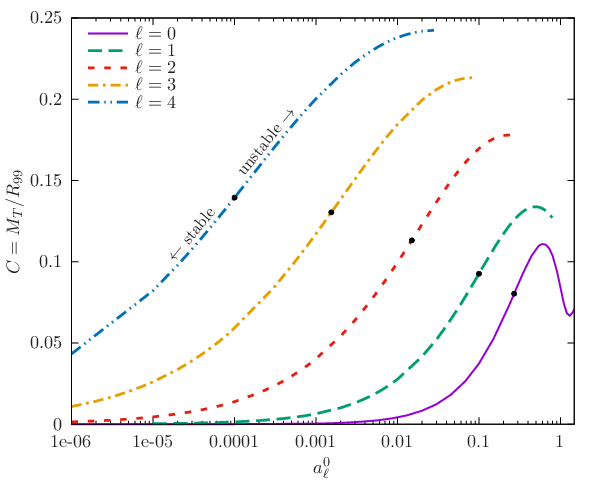
Like in our accompanying work Alcubierre et al. 2019, the total mass and the total boson number , which we define next, will play an important role in the analysis that we present below. Since the theory is invariant under internal transformations, there are conserved current densities, one associated with each generator of the internal symmetry group. Among them, there is one corresponding to the total number of particles minus the antiparticles, given by
| (7) |
which is conserved, . For the spherically symmetric configurations (1,2) analyzed in this work, has vanishing angular components and gives rise to the conserved boson number
| (8) |
where the second integral is restricted to the time-harmonic ansatz (5).
III Linear stability analysis
After having reviewed the most relevant equations of reference Alcubierre et al. 2018, in this section we perform a linear stability analysis of the -boson star ground state configurations. We start in section III.1 by generalizing previous work by Gleiser Gleiser 1988 and by Gleiser and Watkins Gleiser and Watkins 1989 to arbitrary values of , and in this way we derive a coupled wave-like system (the pulsation equations), governing the dynamics of linearized perturbations. By analyzing mode solutions with a harmonic time-dependency, this system reduces to a time-independent system of Schrödinger equations, and in section III.2 we establish several important properties of the corresponding Schrödinger operator. In particular, we show that it is (formally) self-adjoint and discuss some tools that we shall use in this article, such as the generalized nodal theorem Amann and Quittner 1995. Sections III.3, III.4 and III.5 are dedicated to a further analysis of the Schrödinger operator as well as to the asymptotic behavior of the mode solutions in the vicinity of and as . The findings of this section lay the theoretical ground for the numerical results presented in section IV.
III.1 Pulsation equations
In order to derive the pulsation equations it is convenient to write the field amplitude as
| (9) |
where and are real-valued, and where and are the radial function and frequency, respectively, associated with the background solution. Following Gleiser and Watkins 1989, the linearized fields are expanded in the form
| (10a) | |||||
| (10b) | |||||
| (10c) | |||||
| (10d) | |||||
giving rise to small (but time-dependent) variations of the static configurations introduced in the previous section. Here the quantity is related to the linearized mass function via the relation . Note that there is a gauge ambiguity in the definition of the perturbations and , since one can still perform a redefinition of the time coordinate and maintain the same form of the line element as in equation (1). Under an infinitesimal transformation , where is an arbitrary function of time, the fields and remain unaltered, whereas and change according to:
| (11a) | |||||
| (11b) | |||||
We stress that the decomposition (10a,10b) is only valid for the ground state configurations for which has no zeros in the interval . Further below we shall also assume that the linearized fields , , and have a harmonic time-dependency of the form .
Linearizing equations (4a,4b,4c), one obtains the following useful relations between the linearized metric coefficients and scalar fields:
| (12a) | |||||
| (12b) | |||||
| (12c) | |||||
where from now on we omit the subscript on the background quantities to simplify the notation. Eliminating from the first two equations and linearizing the remaining equations (4d,4e), one obtains the following evolution system:
| (13a) | |||||
| (13b) | |||||
which reduce to equations (34) and (35) in Gleiser and Watkins 1989 when (taking into account a different sign convention for the frequency and a factor which was corrected in Hawley and Choptuik 2000). We refer to this system as the pulsation equations in this paper. Note that it relies only on quantities that are invariant under infinitesimal time redefinitions .
To solve equations (13) we need to specify suitable initial data. In order to do so we fix the value of the perturbations of the field defined in equation (9) and its conjugate momentum, , at time ,
| (14a) | |||||
| (14b) | |||||
This determines univocally the initial data for the pulsation equations:
| (15a) | |||||
| (15b) | |||||
| (15c) | |||||
| (15d) | |||||
where
| (16) |
(Remember that is related to through a background function.) In order to obtain we have integrated equation (12b) under the assumption that , a condition that is necessary to guarantee regularity at the origin, and was obtained from the constraint (12a). Once these equations are solved, one acquires by integrating equation (12c), and subsequently is obtained by integrating equations (12a,12b). Note that these two last quantities are defined only up to the gauge ambiguity that we identified in (11).
For practical purposes we will restrict our attention to initial data and that are smooth and of compact support in the interval . Furthermore, we shall require that the initial data satisfies , such that the perturbation does not change the total mass of the system. These conditions imply that and are also compactly supported on and that the total particle number is unaffected. In order to see this more explicitly note that linearizing equation (8) one obtains [cf. equation (37) in Gleiser 1988]
| (17) |
After some manipulations using the constraints (12) and the background equations (4) the integrand in the last expression can be re-written as a total differential, and one obtains the simpler expression
| (18) |
This equation has various important implications. First, it follows that any perturbation for which is bounded at and near yields the relation
| (19) |
between the total particle number and total mass. In particular, it follows for such perturbations that if and only if , and hence the class of compactly supported initial data described above leaves both the total particle number and mass invariant (to linear order in the perturbation). A further consequence of equation (19) (when applied to the solution curves of static -boson stars) is that the total particle number and mass as functions of have the same critical points, and this explains why the location of the extrema of and coincide (see figures 1 in Gleiser 1988; Gleiser and Watkins 1989 for the case, and figure 1 in Alcubierre et al. 2019 for -boson stars with ). Another consequence of equation (19) is that the first variation of the binding energy satisfies . Since this implies that a maximum of corresponds to a minimum of and the other way around. Finally, and most importantly for the purpose of this article, the existence of static perturbations at such extrema signals (but does not prove) the existence of mode solutions to the linearized equations which transition from stable to unstable, see the discussions in section 4 of reference Gleiser and Watkins 1989 and in section IV.2 below.
III.2 Spectral properties and nodal theorem
An alternative way of writing the pulsation equations is based on the original work in Gleiser 1988 where the new quantities and are introduced, which are related to and through the expressions22 2 Note that according to equation (12a). Also the perturbation of the boson number, equation (18), can be expressed in the more compact form [cf. equation (38) in Gleiser 1988] .
| (20) |
The system for can be written in the form
| (21) |
with the matrices , and given by
| (22) |
and the functions , , defined by
| (23a) | |||||
| (23b) | |||||
| (23c) | |||||
Equation (21) has the form , with the Schrödinger-type operator given by
| (24) |
Due to the fact that the matrix is symmetric positive definite and that the matrix is symmetric, the operator is formally self-adjoint with respect to the scalar product
| (25) |
This means that satisfies
| (26) |
for all sufficiently smooth functions and which are compactly supported on the interval , or, more generally, which satisfy appropriate boundary conditions at and as . (We shall analyze these conditions further below.) Since commutes with complex conjugation, it follows from von Neumann’s theorem (see Theorem X.3 in Reed and Simon 1980a) that possesses a self-adjoint extension. This offers the possibility of studying the dynamics of the pulsation equation (21) using the powerful tools of spectral theory for self-adjoint operators, for which there exists a vast literature, see for instance Reed and Simon 1980b; Reed and Simon 1980c.
The precise determination of the appropriate self-adjoint extension of and its properties lie way beyond the scope of this article. Instead, in what follows, we shall focus on the point spectrum of the operator (i.e. its eigenvalues and eigenfunctions), which in an analogous quantum mechanical problem would correspond to the energy levels of the bound states. In our scenario, each negative eigenvalue gives rise to a pair of mode solutions of proportional to which are exponentially growing or decaying in time, and thus a negative eigenvalue implies the instability of the system. On the other hand, each positive eigenvalue of corresponds to a pair of purely oscillating modes proportional to .
One of the useful tools we shall apply in the next section is the nodal theorem by Amann and Quittner Amann and Quittner 1995, which allows one to determine the number of negative eigenvalues of by counting the zeros of a certain determinant which is constructed from two linearly independent zero modes of . More precisely, one solves the differential system with initial data and , , with two linearly independent vectors and in . Then, for small enough and large enough, the number of zeros of the determinant function on the interval is equal to the number of bound states with negative energy (counted with multiplicities) of the operator . The number of zeros is independent of and , provided is sufficiently close to and sufficiently large. Moreover, the number of zeros is independent of the choice of the basis vectors and .
In addition to determining the number of negative eigenvalues of (which correspond to the number of unstable, exponentially in time growing mode solutions of the pulsation equations), we shall also compute numerically the eigenvalues of by means of a shooting algorithm. Since is formally self-adjoint, is either real or purely imaginary. In the latter case, the norm of determines the growth rate of the unstable mode, while in the former case it determines the oscillatory frequency of the mode solutions, which will be compared to the results from a nonlinear numerical time evolution in section IV.
III.3 Transformation of the Schrödinger operator to a simpler form
The application of the nodal theorem requires the satisfaction of certain hypotheses we would like to comment on. To this purpose, we first transform the Schrödinger operator to a simpler form in which the first-derivative terms are eliminated and the transformed operator is formally self-adjoint with respect to the usual scalar product for square-integrable (-) functions. This new form will also simplify the analysis for the asymptotic behavior of the mode solutions in the limits and .
The transformation we apply is with
| (27) |
where is a rotation matrix given by
| (28) |
This transforms the problem into , in which the new operator has the structurally simpler form
| (29) |
with the symmetric matrix given by
| (30) |
where
| (31) |
and denotes the identity matrix. Note that the transformed operator is formally self-adjoint with respect to the standard scalar product
| (32) |
More generally, one has the identity
| (33) |
for any pair of twice continuously differentiable functions and on , and the boundary term vanishes if and are zero at and decay sufficiently rapidly as . It is simple to verify that these conditions are automatically satisfied for the type of initial data specified towards the end of section III.1, and hence the initial data belongs to the class of functions for which the operator is self-adjoint.
Next, we note that the function appearing between the derivative operators in equation (29) is smooth, strictly positive and possesses the limits and as and , respectively. Furthermore, as follows from the results presented in the next two subsections, the transformed potential is smooth on , uniformly bounded near infinity, and near it has the form given in equation (40) below with the matrix coefficient being nonnegative. The only additional assumptions made by the nodal theorem Amann and Quittner 1995 are the requirements that the essential spectrum of contains no negative values and that has only a finite number of negative eigenvalues.33 3 See Reed and Simon 1980b for a definition of the essential spectrum of an operator and Reed and Simon 1980c for theorems on its properties and estimates on the number of bound states. The strict verification of these last two conditions goes beyond the scope of this article; however, the numerical results presented in the next section offer a picture that is fully consistent with the results from the nodal theorem.
In the following, we analyze the asymptotic behavior of the effective potential for and , and the corresponding behavior of the mode solutions.
III.4 Asymptotic behavior for
As has been discussed in Alcubierre et al. 2018, the background solution has the following behavior near the center :
| (34a) | |||||
| (34b) | |||||
| (34c) | |||||
for some positive constants and , with related to the previously defined quantity through the relation . The expressions above include the next-to-leading order terms which will be required for the analysis in this subsection and the appendix. They can be computed from the background equations (17a–17c) in Alcubierre et al. 2018. In particular, the coefficient in equation (34c) can be determined by taking the limit of the right-hand side of equation (17c) in Alcubierre et al. 2018, giving
| (35) |
It follows from equations (34a,34b) and the definition of in equation (28) that
| (36) |
for all .
After these preliminary remarks regarding the properties of the background solution near , we analyze the behavior of the solutions to the mode equation . For the remaining of this subsection, we only compute the leading order terms in and . Higher-order contributions (which are required for the numerical shooting algorithm used in the next section) are worked out in the appendix. First, it follows from equations (28) and (36) that
| (37) |
Next, from equations (23a–23c) one easily finds
| (38) |
and from equation (31),
| (39) |
from which one finally obtains
| (40) |
Note that the matrix coefficient in front of the term on the right-hand side has nonnegative eigenvalues for all , which is one of the hypothesis in the nodal theorem of reference Amann and Quittner 1995. Furthermore, it follows from the regularity of at and from equation (40) that the equation has a regular singular point at , with four linearly independent solutions which behave as
| (41) |
in the vicinity of . The physical relevant ones (i.e. those leading to perturbations , , and that remain finite near the origin) give rise to the two-parameter family of solutions
| (42) |
with free constants and . In terms of the fields and appearing in the original system (13a,13b) this leads to local solutions of the form (cf. equation (20))
| (43a) | |||||
| (43b) | |||||
with free constants and . Note that the latter appears only in the correction term in the expansion. A consistent expansion (needed for the numerical implementation in the next section) which includes the and correction terms in both fields will be given in the appendix. Finally, we note that the conditions (42) guarantee that the boundary terms in equations (18) and (33) vanish at .
III.5 Asymptotic behavior at
As , the background metric fields and both converge to one while the background scalar field quantity decays exponentially to zero. Therefore, for large one can replace and by their Schwarzschild values,
| (44) |
with the total mass. (The error in these formulae is exponentially small, as follows from the background equations (7a) and (7b) in Alcubierre et al. 2018.) Using these expressions in the background equation (7c) in Alcubierre et al. 2018 it then follows that has the following asymptotic expansion at (note that ):
| (45) |
for some constant . In particular, this implies that
| (46) |
from which
| (47) |
and
| (48) |
Therefore,
| (49) |
in equation (30), and it follows that the potential term of the Schrödinger-type operator (29) is uniformly bounded for large , which is also a necessary condition to apply the nodal theorem.
Using equation (49) and the fact that one can rewrite the eigenvalue problem in the form with
For given values of , this problem has asymptotic solutions of the form
| (58) |
with a nonvanishing two-vector , an exponential factor and a constant matrix . Here, refers to the matrix , and its presence is needed in order to eliminate the term appearing in equation (III.5). Introducing the ansatz (58) into the equation , one finds to leading order:
| (59) |
For a nontrivial solution to exist, the determinant of the matrix appearing on the left-hand side must be zero, which yields
| (60) |
with corresponding two-vectors proportional to
| (61) |
(These expressions are equivalent to each other as long as . When , the first expression should be used, for the second one.)
Equation (60) yields four solutions for , which, in general, lie in the complex plane. We are particularly interested in understanding the behavior of the real part of these roots, since they determine whether or not the corresponding mode solution decays as . To analyze this, we first notice that must be real, since it is an eigenvalue of a self-adjoint operator. Thus, must either lie on the real or on the imaginary axis of the complex plane. At the intersection, , we have , so in this case the roots are real, with one degenerated positive and one degenerated negative root. By continuity, for small enough values of there are two roots with positive and two roots with negative real parts. More precisely, when one finds
| (62) |
where all four combinations of the signs are possible, the sign choice inside the square parenthesis corresponding to the sign in equation (60).
Next, it follows from equation (60) and the fact that that the real part of cannot vanish if is purely imaginary. Since depends continuously on , we conclude there are two roots with positive and two roots with negative real parts as long as is purely imaginary. On the other hand, we notice that is real when is real. Assuming without loss of generality that and that , it follows from equation (60) that when for the upper sign and for the lower sign. Hence, for there are two roots with negative real part and two with positive real part, when there is one root with negative and one with positive real part, the remaining two roots being purely imaginary, while for it follows that all the roots are purely imaginary, giving rise to oscillatory modes. We summarize these findings in figure 2.
2 roots with negative real part 2 real negative roots 1 real negative root
2 roots with positive real part 2 real positive roots 1 real positive root
2 purely imaginary roots 4 purely imaginary roots
0
unstable branch stable branch
Translating these results to the function defined in equation (20) by means of the transformation (27), this yields the asymptotic behavior
| (63) |
For small positive it follows from equation (62) that there are three exponentially growing modes and one exponentially decaying mode. By analyzing the sign of the term in equation (60) it is not difficult to show that this behavior persists for , while for all four modes grow exponentially. When the two roots with the positive real parts clearly give rise to exponentially growing modes. The behavior of the remaining two modes are exponentially damped, as can be seen from the quadratic term in equation (62) and the fact the real part of cannot vanish for purely imaginary different from zero. Therefore, for such , there are two exponentially growing and two exponentially decaying modes for . For convenience, we summarize this behavior and the behavior of other fields in table 1.
For completeness, we also provide the result from the next-to-leading order contribution, which yields the following expression for the matrix in equation (58):
| (64) |
When applied to the two-vector in equation (61), this gives
| (65) |
and the solutions at infinity are
| (66) |
To summarize the findings of this section, for there are two linearly independent mode solutions of the pulsation equations which are normalizable at infinity. The corresponding fields decay exponentially to zero as and guarantee that the boundary terms in equations (18) and (33) vanish at . In the next section we show (through numerical calculations) that for certain values of an appropriate linear combination of these two modes can be matched to the boundary condition at the origin, see equation (42), which yields an eigenfunction of the operator . For , the number of independent mode solutions which are normalizable and cancel the boundary terms in equations (18) and (33) at infinity is less clear, since in this case there are solutions whose asymptotics is given by equation (66) with purely imaginary . These modes have a power-law behavior of the type and in principle, one could determine whether or not they are decaying by analyzing the real part of . However, all the numerical eigenvalues found in the next section satisfy , so that we do not pursue this issue further.
| ||||||||||||||||||||||||||||||||||||||||||||||||||||||||||||||||||||||||
IV Results
After having derived the pulsation equations and discussed their most important properties, in this section we determine the number of negative energy bound states and the eigenvalues of the Schrödinger operator by numerical means. Then we compare our results with those obtained from a fully nonlinear numerical evolution of the EKG system Alcubierre et al. 2019.
IV.1 Number of negative energy bound states
As mentioned in section III.2 the system of equations (13) forms a self-adjoint coupled system of radial Schrödinger equations, once the time-dependence is assumed. This fact offers the possibility of studying the point spectrum of the operator given by equation (24) in a way analogous to a quantum mechanical problem. Indeed, in order to find the number of bound states with negative energy it is sufficient to solve which, as already shown, is equivalent to solving equations (13) in the time-independent case . The nodal theorem requires finding two solutions with labeling the following boundary conditions at : and , , with two linearly independent vectors and in . Taking these two vectors to be the standard basis in and translating the boundary conditions to the fields and used in our code by means of equations (20), one obtains
- •
For one imposes , , and .
- •
For one imposes , , and .
By numerically integrating equations (13) with these boundary conditions and , one finally computes the determinant
| (67) |
on the interval , and by counting the number of zeros of one finds the number of unstable modes of the corresponding -boson star solution. We have tested several choices for and to convince ourselves that the number of zeros of is independent of the chosen intervals .
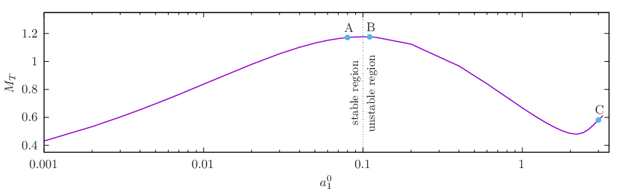
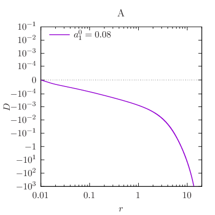
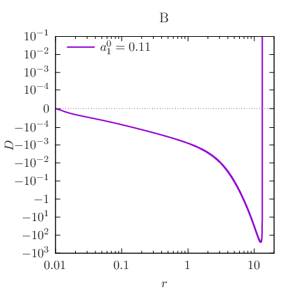
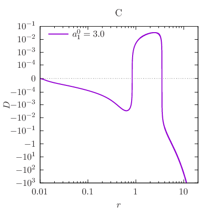
In figure 3 we show our results for -boson stars with . The upper panel of this figure shows the relation between the total mass and the parameter (i.e. the central value of ), with the first maximum of the mass at . Recall from the review in section II that full nonlinear numerical simulations Alcubierre et al. 2019 indicate that configurations with are stable, while those with are unstable. In order to verify that these results are consistent with the nodal theorem, we have chosen one configuration on the stable branch (labeled A and corresponding to ), and two more configurations on the unstable branch (labeled B and C and corresponding to and , respectively). The behavior of the determinant is shown for each of these configurations in the lower panel of figure 3. Observe that is a monotonic decreasing function of for the stable configuration A. No zeros of are found in this case which proves that this configuration is linearly stable, consistent with the results from the numerical simulations. On the other hand, the function for configuration B exhibits one zero, showing that it possesses a single unstable mode. Moreover, configuration C, which lies to the right of the local minimum of , has two unstable modes as can be seen from the plot of in this case. The fact that there is an increasing number of unstable modes as increases and passes through local extrema of the mass will be further discussed in the next subsection, based on the properties of the mode solutions of the pulsation equations.
IV.2 Mode solutions of the pulsation equations
We proceed to find the mode solutions (proportional to ) of the pulsation equations (13) by means of a numerical shooting algorithm. This system describes an eigenvalue problem for the frequency . In order to get a better handle on the solution in the vicinity of , we rescale the variable by a factor proportional to which is motivated by the asymptotic behavior in equation (43b). This yields the new system of equations (70) for the fields and derived in the appendix. We numerically integrate this system from outwards, starting with the boundary conditions at given by equations (82) in the appendix, and fine-tune the values of and the free parameter in equation (82a) until the boundary conditions at discussed in section III.5 are satisfied. In practice, this is achieved by choosing an outer radius , which is the largest radius where the integration is performed, and by imposing the boundary conditions at . In terms of the code variables and these conditions are equivalent to demanding (since )
| (68a) | |||||
| (68b) | |||||
at .44 4 Theoretically, the boundary conditions (68) are equivalent to setting at . However, we have found that the former work much better in practice. In summary, finding the mode solutions of the pulsation equations leads to an eigenvalue problem for , for which the solutions must be consistent with both boundary conditions at and The double shooting algorithm thus finds both the value of and the value of the free parameter in equation (82a) to satisfy correctly the boundary conditions. The value of is increased until the values of and have converged within a tolerance value of . Some examples showing the values for and for different configurations with are shown in table 2.
| 1 | ||||
|---|---|---|---|---|
| 1 | ||||
| 1 | ||||
| 1 | ||||
| 1 | ||||
| 1 | ||||
| 1 | ||||
| 1 | ||||
| 2 | ||||
| 2 | ||||
| 2 | ||||
| 2 | ||||
| 2 | ||||
| 2 | ||||
| 2 | ||||
| 2 |
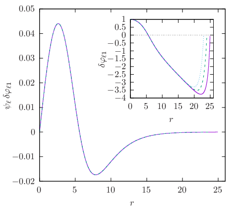
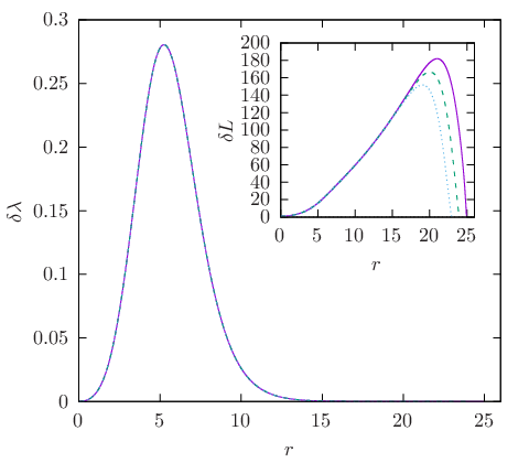
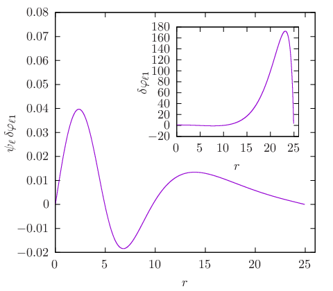
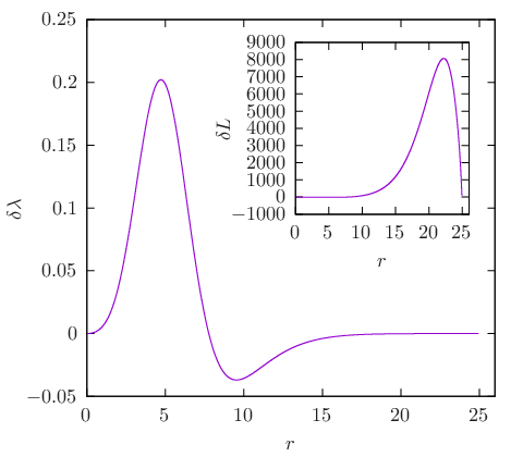
For each -boson star characterized by and we find a discrete family of mode solutions to the pulsation equations which is characterized by the number of nodes , , of the field in the interval . The increasing number of nodes is associated with an increasing value for , i.e. , with the frequency of the corresponding mode. Hence, similar to the properties of the background solution describing the -boson star, for the solutions of the pulsation equations there are ground, , and excited states, . The typical radial dependence of these linear modes is shown in figures 4 and 5 for the particular case of and . The solution shown in figure 4 is the one with zero nodes in (the ground state), while the solution with one node in (the first excited state) is plotted in figure 5. The radial dependence of the linear modes with and are qualitatively similar to those with and .
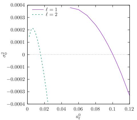
Next, we compare the eigenvalue for the modes with zero nodes and with the corresponding modes with . The results are shown in figure 6 where we show the value of as a function of . Table 2 presents the same results as in figure 6 for a more detailed list of values obtained for . As can be seen from figure 6 and table 2, the configurations with have positive values of which correspond to a pair of oscillating modes which do not grow in time.55 5 Recall that each eigenvalue gives rise to a pair of mode solutions of the form and . However, when , is negative which gives rise to a pair of modes, one being exponentially growing in time and the other exponentially damped, showing that the corresponding -boson star is linearly unstable. The configuration corresponding to the threshold value describes a static mode with , and since by construction our modes are restricted to spherically symmetric configurations which preserve the total mass (and particle number), this mode must represent a linearized solution along the -boson star configurations at a point where the first variation of the mass is zero (cf. Gleiser and Watkins 1989). In fact, it turns out that the threshold value corresponds precisely to the value of the maximum mass configuration. These results explain the reason behind the transition stable-unstable at the first maximum of the mass that we pointed out in figure 1, and are fully compatible with the results from the full nonlinear numerical evolution of the -boson star configurations performed in Alcubierre et al. 2019.
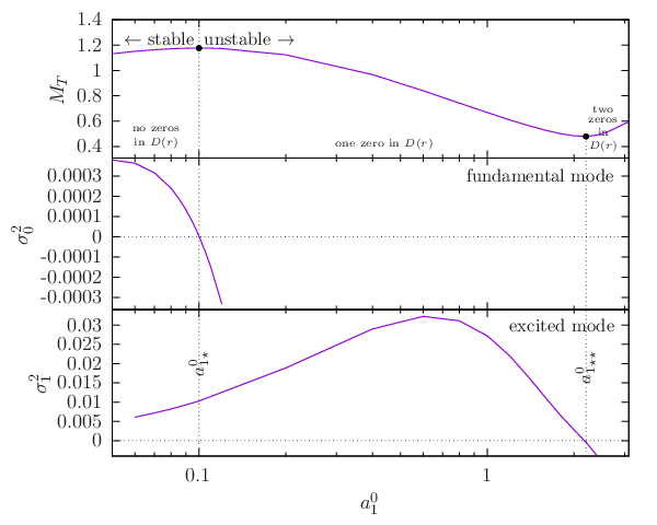
We conclude this subsection by commenting on the origin of the number of instabilities that the nodal theorem is counting, based on the mode solutions to the pulsation equations. As we have mentioned, it is possible to find solutions to the pulsation equations with nodes of the function . For instance, in figure 7 we have plotted and for configurations with as a function of . For comparison, the top panel of figure 7 shows once more the total mass as a function of . As discussed above, the ground state eigenvalue is positive for , which means that the corresponding -boson star is stable under linear radial perturbation. In fact, the nodal theorem shows that the function has no zeros for (cf. configuration A in figure 3) showing that there are, in fact, no unstable modes in this region. For , becomes negative, the corresponding -boson star is unstable, and the nodal theorem shows that has at least one zero in this region (cf. configurations B and C in figure 3). Next, let us examine the behavior of the first excited eigenvalue as a function of (see the lower panel of figure 7). Note that is positive for values where corresponds to the configuration for which has its first local minimum. This means that there are no additional unstable modes in this region, a fact that is confirmed by the results from the nodal theorem that show that has only one zero for (cf. configurations B in figure 3). However, for the eigenvalue becomes negative meaning that in this region the configuration has two exponentially in time growing modes (one which is due to and another one due to ), a fact that is again confirmed by the nodal theorem (cf. configurations C in figure 3). From this picture, we conjecture that as increases, the corresponding -boson star acquires one additional unstable mode each time crosses an extremum of the mass.
IV.3 Comparison of linear perturbation theory with numerical perturbations of -boson stars
In this subsection we compare the results of the perturbation theory with those of a full non-linear numerical evolution of a perturbed -boson star in the stable branch.
For our perturbed initial data we follow the procedure described in Alcubierre et al. 2019. We start from a solution corresponding to a stationary -boson star and add a small, but finite, perturbation. The perturbation is constructed in such a way that the initial momentum density remains zero, in order to guarantee that the momentum constraint is trivially satisfied. Also, we choose a perturbation such that the local boson density does not change at , that is we keep constant in equation (8). We then solve again the Hamiltonian constraint in order to have fully consistent initial data and evolve the full EKG system numerically in time. Notice that keeping fixed the local boson density does not in fact keep the total boson number conserved, as the volume element will change once we solve again the Hamiltonian constraint. Basically, when constructing our initial data we are ignoring the term in equation (17). This changes slightly the background solution that we need to compare with the results of our numerical evolution, but the effects are so small that they are negligible for practical purposes, as we have corroborated.
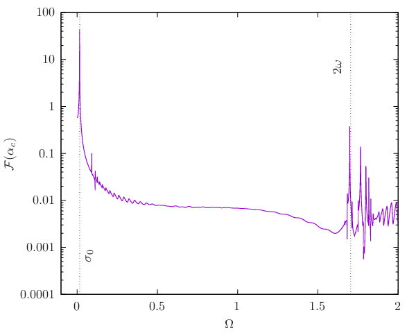
We perform a very long time evolution in order to have a large number of oscillations of the system. To find the frequencies of the perturbed -boson star, we Fourier transform the value of the lapse function at the origin. Notice that for an unperturbed star this value should remain constant. Using a fast Fourier transform (FFT), we then compute the power spectrum of .
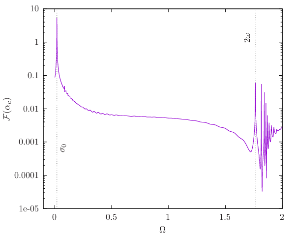
Figure 8 shows the power spectrum of for the time interval for the case of a perturbed -boson star with , and two different values of corresponding to the background configurations in the first two rows of table 2. The power spectrum clearly indicates there are several frequencies at which the system oscillates. The largest (leftmost) peak in both cases corresponds to the value of whose square is given in table 2, that is the fundamental mode of the perturbation analysis. The second dominant frequency corresponds to twice the frequency of the original unperturbed -boson star. The reason for this is that the lapse function (as well as other metric quantities) depends on the energy density of the field, which is proportional to its square modulus, so it oscillates with twice the frequency.
The other peaks present in the power spectrum seem to correspond to linear combinations of twice the values of the overtones of the -boson star (or the first two excited states) and halves of . At this point we do not have a clear understanding of exactly why these particular combinations appear in the spectrum, but they would seem to originate in the nonlinear coupling among the different modes and depend on the initial perturbation. A further analysis of the exact modes that are excited is beyond the scope of the present work.
V Conclusions
-boson stars Alcubierre et al. 2018 are a generalization of the standard boson stars with which are obtained from a collection of an arbitrary odd number of complex massive scalar fields with an internal symmetry. Even if spherical as a whole, the individual scalar fields are described by an eigenstate of the angular momentum operator with angular momentum number , with fields belonging to different azimuthal number having the same amplitude . The resulting configurations are described by regular, asymptotically flat, static and spherically symmetric solutions to the classical EKG system, and they can be parametrized by , an excitation number that counts the number of nodes of the wave function, and a continuous finite parameter representing the amplitude of the radial function at the origin.
In order to have a possible phenomenological impact, -boson stars need to be dynamically stable as solutions of the EKG equations. In this paper, by means of a linear perturbation analysis, we have studied the stability of -boson stars by analyzing the time evolution of linearized radial perturbations which conserve the total number of particles and mass. Our results support the previous findings of our numerical study in Alcubierre et al. 2019 by confirming that for a given , nodeless -boson stars are stable if is smaller than a critical value which corresponds to the maximum mass configuration.
The existence of a branch of solutions that is stable under linear perturbations was confirmed in this work by two different methods:
- 1.
On the one hand we have derived the pulsation equations that describe the evolution of the linearized radial perturbations to the -boson star ground state configurations. These equations form a self-adjoint coupled system of Schrödinger equations, which is then suitable to the applicability of the generalized nodal theorem Amann and Quittner 1995. This theorem allows one to count the number of unstable modes of the pulsation equations by counting the number of zeros of a certain determinant function constructed from two independent zero modes. As we have shown, the configurations with have no unstable modes while those with have one, two or more unstable modes for the cases we have computed. Furthermore, the number of unstable modes associated with the configuration coincides with the number of critical points of the function in the interval (0, ). See figure 3 for details.
- 2.
On the other hand, we have solved the pulsation equations for solutions with a harmonic time dependency of the form by means of a numerical shooting algorithm. The mode solutions reveal that the linear radial perturbation of those -boson stars with oscillates with a real frequency around the background configuration. In contrast, configurations with possess linear modes growing exponential in time, for the cases we have analyzed. In particular, our analysis allows us to compute numerically the frequency for the stable configuration (see figure 7), and we have found that this frequency correctly predicts the position of the highest peak in the Fourier spectrum of a perturbation obtained by numerically evolving the nonlinear EKG system (see figure 8).
Our results based on the nodal theorem and the computation of the mode solutions of the pulsation equations complement each other. The counting of the number of instabilities makes sure that no unstable modes have been missed in our shooting algorithm, and in particular shows the existence of a stable configurations, whereas the computation of the mode solutions allows one to compute the spectrum of frequencies associated with the perturbations. Furthermore, the number of instabilities given by the nodal theorem corresponds to the number of the linear perturbations that grow in time exponentially.
Our results confirm that the pulsation equations capture the dynamics of the evolution of -boson stars. All the results presented here, together with the numerical studies presented in Alcubierre et al. 2019, suggest that -boson stars do have a branch which is stable, at least with respect to radial perturbations, thus making them suitable to model astrophysical objects.
If ultimately proven to be stable also with respect to non-spherical perturbations, confirming the findings in Jaramillo et al. 2020, one would have compact objects made of scalar fields that are stable and that can have compactness larger than standard boson stars, as shown in figure 1. The astrophysical implications of these compact structures are still unknown. However, they should be of considerable interest for those dark matter models which are described by a (zero spin) scalar field.
Acknowledgements.
This work was partially supported by CONACyT Ciencia de Frontera Projects No. 376127 “Sombras, lentes y ondas gravitatorias generadas por objetos compactos astrofísicos”, and No. 304001 ”Estudio de campos escalares con aplicaciones en cosmología y astrofísica”, as well as DGAPA-UNAM grants IN110218 and IN105920. OS was partially supported by a CIC grant to Universidad Michoacana de San Nicolás de Hidalgo. ADT was partially suported by CONACyT grant No. 286897.Appendix. The pulsation equations in a form more suitable for numerical integration
As discussed in section IV the computation of the eigenvalues and the associated linearized modes is based on a numerical shooting algorithm which integrates the pulsation equations outwards starting from the origin . To this purpose, and taking into account the asymptotic behavior of the fields near , see equation (43), it is convenient to replace with the rescaled quantity
| (69) |
After this rescaling, equations (13a,13b) assume the following form:
where we have introduced the shortcut notation and set , taking into account that the background field scales like near , see equation (34c). In these expressions, we eliminate the derivatives of the metric coefficients using the background equations (17a) and (17b) in reference Alcubierre et al. 2018 and
| (71) |
where here and its first two derivatives can be computed from and equation (17c) in Alcubierre et al. 2018.
The system (70) is singular at ; however, as we have shown in section III.4 there is a two-parameter family of solutions which are regular at the origin. To find the corresponding expansions of these solutions which can be used to start the numerical integration, we write the system (70) in the form
| (72) |
and look for solutions of the form
| (73) |
near . It follows from equations (34) that the matrix-valued functions and have expansions of the following form:
| (74) |
with constant matrices and . Substituting the expansion (73) into equation (72) leads to
| (75) |
Since
| (76) |
and
| (77) |
it follows from the first relation in equation (75) that
| (78) |
for some real coefficient , while the second relation in equation (75) leads to
| (79) |
The matrix on the left-hand side is not invertible, meaning that needs to lie in its image and that contains an additional free parameter. A careful calculation reveals that for all ,
| (80) |
which means that the system (79) is solvable with
| (81) |
This finally leads to the following expansion near (setting without loss of generality)
| (82a) | |||||
| (82b) | |||||
with a free coefficient. For we may redefine
| (83) |
and the resulting expansion seems to agree with the one in equation (38) in Gleiser and Watkins 1989 (taking into account that and ).
References
- Kaup (1968) D. J. Kaup, Phys. Rev. 172, 1331 (1968).
- Ruffini and Bonazzola (1969) R. Ruffini and S. Bonazzola, Phys. Rev. 187, 1767 (1969).
- Jetzer (1992) P. Jetzer, Phys. Rep. 220, 163 (1992).
- Schunck and Mielke (2003) F. E. Schunck and E. W. Mielke, Class. Quantum Grav. 20, R301 (2003), eprint 0801.0307.
- Liebling and Palenzuela (2012) S. L. Liebling and C. Palenzuela, Living Rev.Rel. 15, 6 (2012), eprint 1202.5809.
- Schunck and Mielke (1996) F. E. Schunck and E. W. Mielke, in Relativity and Scientific Computing. Computer Algebra, Numerics, Visualization (1996), pp. 138–151.
- Yoshida and Eriguchi (1997) S. Yoshida and Y. Eriguchi, Phys. Rev. D 56, 762 (1997).
- Palenzuela et al. (2017) C. Palenzuela, P. Pani, M. Bezares, V. Cardoso, L. Lehner, and S. Liebling, Phys. Rev. D 96, 104058 (2017), eprint 1710.09432.
- Seidel and Suen (1994) E. Seidel and W.-M. Suen, Phys. Rev. Lett. 72, 2516 (1994), eprint gr-qc/9309015.
- Sanchis-Gual et al. (2019) N. Sanchis-Gual, F. Di Giovanni, M. Zilhão, C. Herdeiro, P. Cerdá-Durán, J. A. Font, and E. Radu, Phys. Rev. Lett. 123, 221101 (2019), eprint 1907.12565.
- Alcubierre et al. (2018) M. Alcubierre, J. Barranco, A. Bernal, J. C. Degollado, A. Diez-Tejedor, M. Megevand, D. Nunez, and O. Sarbach, Class. Quant. Grav. 35, 19LT01 (2018), eprint 1805.11488.
- Olabarrieta et al. (2007) I. Olabarrieta, J. F. Ventrella, M. W. Choptuik, and W. G. Unruh, Phys. Rev. D76, 124014 (2007), eprint 0708.0513.
- Gleiser (1988) M. Gleiser, Phys. Rev. D38, 2376 (1988), [Erratum: Phys. Rev.D39,no.4,1257(1989)].
- Gleiser and Watkins (1989) M. Gleiser and R. Watkins, Nucl. Phys. B319, 733 (1989), eprint gr-qc/9905067.
- T. D. Lee (1989) P. Y. T. D. Lee, Nucl. Phys B315, 447 (1989).
- Balakrishna et al. (1998) J. Balakrishna, E. Seidel, and W.-M. Suen, Phys. Rev. D 58, 104004 (1998), eprint gr-qc/9712064.
- Seidel and Suen (1990) E. Seidel and W. Suen, Phys. Rev. D42, 384 (1990).
- Hawley and Choptuik (2000) S. Hawley and M. Choptuik, Phys. Rev. D62, 104024 (2000), eprint gr-qc/0007039.
- Guzman (2009) F. Guzman, Revista Mexicana de Fisica 55, 321 (2009).
- Kusmartsev et al. (1991) F. V. Kusmartsev, E. W. Mielke, and F. E. Schunck, Phys. Rev. D 43, 3895 (1991), eprint 0810.0696.
- Chandrasekhar (1964a) S. Chandrasekhar, Phys. Rev. Lett. 12, 114 (1964a).
- Chandrasekhar (1964b) S. Chandrasekhar, Astrophys. J. 140, 417 (1964b), [Erratum: Astrophys.J. 140, 1342 (1964)].
- Shapiro and Teukolsky (1983) S. L. Shapiro and S. A. Teukolsky, Black holes, white dwarfs, and neutron stars: The physics of compact objects (1983), ISBN 978-0-471-87316-7.
- Alcubierre et al. (2019) M. Alcubierre, J. Barranco, A. Bernal, J. C. Degollado, A. Diez-Tejedor, M. Megevand, D. Núñez, and O. Sarbach, Class. Quant. Grav. 36, 215013 (2019), eprint 1906.08959.
- Jaramillo et al. (2020) V. Jaramillo, N. Sanchis-Gual, J. Barranco, A. Bernal, J. C. Degollado, C. Herdeiro, and D. Núñez, Phys. Rev. D 101, 124020 (2020), eprint 2004.08459.
- Sanchis-Gual et al. (2021) N. Sanchis-Gual, F. Di Giovanni, C. Herdeiro, E. Radu, and J. A. Font (2021), eprint gr-qc/2103.12136.
- Amann and Quittner (1995) H. Amann and P. Quittner, J. Math. Phys. 36, 4553 (1995).
- Reed and Simon (1980a) M. Reed and B. Simon, Methods of Modern Mathematical Physics, Vol. II: Fourier Analysis, Self-Adjointness (Academic Press, San Diego, 1980a).
- Reed and Simon (1980b) M. Reed and B. Simon, Methods of Modern Mathematical Physics, Vol. I: Functional Analysis (Academic Press, San Diego, 1980b).
- Reed and Simon (1980c) M. Reed and B. Simon, Methods of Modern Mathematical Physics, Vol. IV: Analysis of Operators (Academic Press, San Diego, 1980c).