LiBRe: A Practical Bayesian Approach to Adversarial Detection
Abstract
Despite their appealing flexibility, deep neural networks (DNNs) are vulnerable against adversarial examples. Various adversarial defense strategies have been proposed to resolve this problem, but they typically demonstrate restricted practicability owing to unsurmountable compromise on universality, effectiveness, or efficiency. In this work, we propose a more practical approach, Lightweight Bayesian Refinement (LiBRe), in the spirit of leveraging Bayesian neural networks (BNNs) for adversarial detection. Empowered by the task and attack agnostic modeling under Bayes principle, LiBRe can endow a variety of pre-trained task-dependent DNNs with the ability of defending heterogeneous adversarial attacks at a low cost. We develop and integrate advanced learning techniques to make LiBRe appropriate for adversarial detection. Concretely, we build the few-layer deep ensemble variational and adopt the pre-training & fine-tuning workflow to boost the effectiveness and efficiency of LiBRe. We further provide a novel insight to realise adversarial detection-oriented uncertainty correction without inefficiently crafting adversarial examples during training. Extensive empirical studies covering a wide range of scenarios verify the practicability of LiBRe. We also conduct thorough ablation studies to evidence the superiority of our modeling and learning strategies.11 1 Code at https://github.com/thudzj/ScalableBDL.
1 Introduction
The blooming development of deep neural networks (DNNs) has brought great success in extensive industrial applications, such as image classification [23], face recognition [9] and object detection [50]. However, despite their promising expressiveness, DNNs are highly vulnerable to adversarial examples [57, 19], which are generated by adding human-imperceptible perturbations upon clean examples to deliberately cause misclassification, partly due to their non-linear and black-box nature. The threats from adversarial examples have been witnessed in a wide spectrum of practical systems [52, 12], raising an urgent requirement for advanced techniques to achieve robust and reliable decision making, especially in safety-critical scenarios [13].
Though increasing methods have been developed to tackle adversarial examples [42, 69, 25, 18, 68], they are not problemless. On on hand, as one of the most popular adversarial defenses, adversarial training [42, 69] introduces adversarial examples into training to explicitly tailor the decision boundaries, which, yet, causes added training overheads and typically leads to degraded predictive performance on clean examples. On the other hand, adversarial detection methods bypass the drawbacks of modifying the original DNNs by deploying a workflow to detect the adversarial examples ahead of decision making, by virtue of auxiliary classifiers [44, 18, 68, 5] or designed statistics [14, 40]. Yet, they are usually developed for specific tasks (e.g., image classification [68, 32, 18]) or for specific adversarial attacks [39], lacking the flexibility to effectively generalize to other tasks or attacks.
By regarding the adversarial example as a special case of out-of-distribution (OOD) data, Bayesian neural networks (BNNs) have shown promise in adversarial detection [14, 38, 54]. In theory, the predictive uncertainty acquired under Bayes principle suffices for detecting heterogeneous adversarial examples in various tasks. However, in practice, BNNs without a sharpened posterior often present systematically worse performance than their deterministic counterparts [61]; also relatively low-cost Bayesian inference methods frequently suffer from mode collapse and hence unreliable uncertainty [15]. BNNs’ requirement of more expertise for implementation and more efforts for training than DNNs further undermine their practicability.
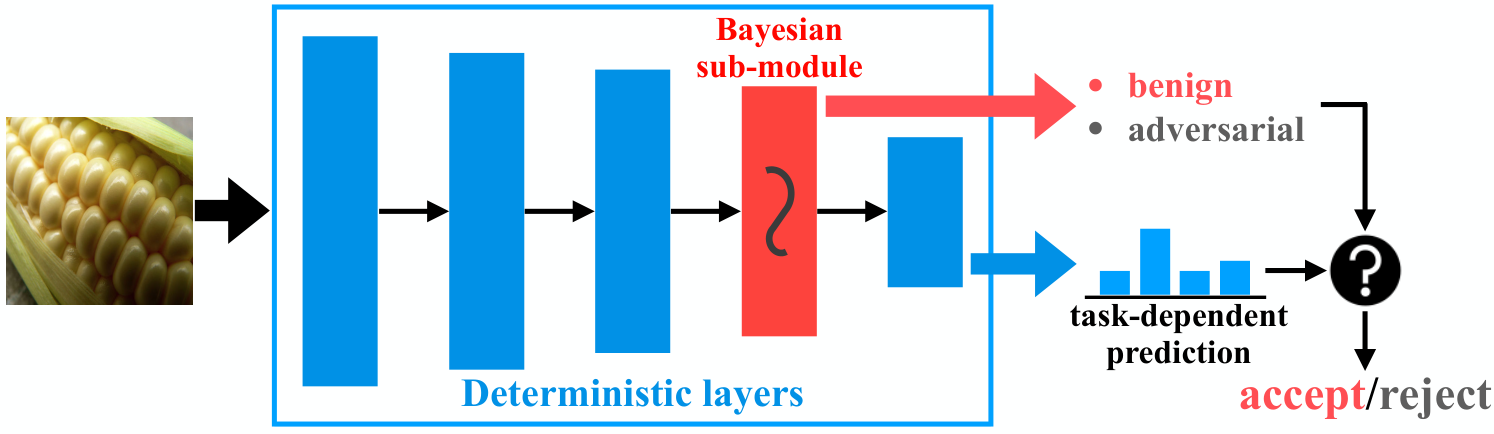
In the work, we aim to develop a more practical adversarial detection approach by overcoming the aforementioned issues of BNNs. We propose Lightweight Bayesian Refinement (LiBRe), depicted in Fig. 1, to reach a good balance among predictive performance, quality of uncertainty estimates and learning efficiency. Concretely, LiBRe follows the stochastic variational inference pipeline [2], but is empowered by two non-trivial designs: (i) To achieve efficient learning with high-quality outcomes, we devise the Few-lAyer Deep Ensemble (FADE) variational, which is reminiscent of Deep Ensemble [31], one of the most effective Bayesian marginalization methods [62], and meanwhile inspired by the scalable last-layer Bayesian inference [29]. Namely, FADE only performs deep ensemble in the last few layers of a model due to their crucial role for determining model behaviour, while keeps the other layers deterministic. To encourage various ensemble candidates to capture diverse function modes, we develop a stochasticity-injected learning principle for FADE, which also benefits to reduce the gradient variance of the parameters. (ii) To further ease and accelerate the learning, we propose a Bayesian refinement paradigm, where we initialize the parameters of FADE with the parameters of its pre-trained deterministic counterpart, thanks to the high alignment between FADE and point estimate. We then perform fine-tuning to constantly improve the FADE posterior.
As revealed by [22], the uncertainty quantification purely acquired from Bayes principle may be unreliable for perceiving adversarial examples, thus it is indispensable to pursue an adversarial detection-oriented uncertainty correction. For universality, we place no assumption on the adversarial examples to detect, so we cannot take the common strategy of integrating the adversarial examples crafted by specific attacks into detector training [40]. Alternatively, we cheaply create uniformly perturbed examples and demand high predictive uncertainty on them during Bayesian refinement to make the model be sensitive to data with any style of perturbation. Though such a correction renders the learned posterior slightly deviated from the true Bayesian one, it can significantly boost adversarial detection performance.
The task and attack agnostic designs enable LiBRe to quickly and cheaply endow a pre-trained task-dependent DNN with the ability to detect various adversarial examples when facing new tasks, as testified by our empirical studies in Sec 5. Furthermore, LiBRe has significantly higher inference (i.e., testing) speed than typical BNNs thanks to the adoption of lightweight variational. We can achieve further speedup by exploring the potential of parallel computing, giving rise to inference speed close to the DNN in the same setting. Extensive experiments in scenarios ranging from image classification, face recognition, to object detection confirm these claims and testify the superiority of LiBRe. We further perform thorough ablation studies to deeply understand the adopted modeling and learning strategies.
2 Related Work
Detecting adversarial examples to bypass their safety threats has attracted increasing attention recently. Many works aim at distinguishing adversarial examples from benign ones via an auxiliary classifier applied on statistical features [18, 68, 5, 7, 65]. [21] introduces an extra class in the classifier for adversarial examples. Some recent works exploit neighboring statistics to construct more powerful detection algorithms: [32] fits a Gaussian mixture model of the network responses, and resorts to the Mahalanbobis distance for adversarial detection in the inference phase; [40] introduces the more advanced local intrinsic dimensionality to describe the distance distribution and observes better results. RCE [47] is developed with the promise of leading to an enhanced distance between adversarial and normal images for kernel density [14] based detection. However, most of the aforementioned methods are restricted in the classification scope, and the detectors trained against certain attacks may not effectively generalize to unseen attacks [39].
Bayesian deep learning [20, 60, 2, 1, 36, 26] provides us with a more theoretically appealing way to adversarial detection. However, though the existing BNNs manage to perceive adversarial examples [14, 49, 54, 38, 48, 33], they are typically limited in terms of training efficiency, predictive performance, etc., and thus cannot effectively scale up to real-world settings. More severely, the uncertainty estimates given by the BNNs for adversarial examples are not always reliable [22], owing to the lack of particular designs for adversarial detection. In this work, we address these issues with elaborated techniques and establish a more practical adversarial detection approach.
3 Background
In this section, we motivate Lightweight Bayesian Refinement (LiBRe) by briefly reviewing the background of adversarial defense, and then describe the general workflow of Bayesian neural networks (BNNs).
3.1 Adversarial Defense
Typically, let denote a collection of training samples with and as the input data and label, respectively. A deep neural network (DNN) parameterized by is frequently trained via maximum a posteriori estimation (MAP):
| (1) |
where refers to the predictive distribution of the DNN model. By setting the prior as an isotropic Gaussian, the second term amounts to the L2 (weight decay) regularizer with a tunable coefficient in optimization. Generally speaking, the adversarial example corresponding to against the model is defined as
| (2) |
where is the valid perturbation set with as the perturbation budget and as some norm (e.g., ). Extensive attack methods have been developed with promise to solve the above minimization problem [19, 41, 4, 58], based on gradients or not.
The central goal of adversarial defense is to protect the model from making undesirable decisions for the adversarial examples . A representative line of work approaches this objective by augmenting the training data with on-the-fly generated adversarial examples and forcing the model to yield correct predictions on them [42, 69]. But their limited training efficiency and compromising performance on clean data pose a major obstacle for real-world adoption. As an alternative, adversarial detection methods focus on distinguishing the adversarial examples from the normal ones so as to bypass the potentially harmful outcomes of making decisions for adversarial examples [44, 5, 40]. However, satisfactory transferability to unseen attacks and tasks beyond image classification remains elusive [39].
3.2 Bayesian Neural Networks
In essence, the problem of distinguishing adversarial examples from benign ones can be viewed as a specialized out-of-distribution (OOD) detection problem of particular concern in safety-sensitive scenarios – with the model trained on the clean data, we expect to identify the adversarial examples from a shifted data manifold, though the shift magnitude may be subtle and human-imperceptible. In this sense, we naturally introduce BNNs into the picture attributed to their principled OOD detection capacity along with the equivalent flexibility for data fitting as DNNs.
Modeling and training. Typically, a BNN is specified by a parameter prior and an NN-instantiated data likelihood . We are interested in the parameter posterior instead of a point estimate as in DNN. It is known that precisely deriving the posterior is intractable owing to the high non-linearity of neural networks. Among the wide spectrum of approximate Bayesian inference methods, variational BNNs are particularly attractive due to their close resemblance to standard backprop [20, 2, 37, 55, 56, 53, 46]. Generally, in variational BNNs, we introduce a variational distribution with parameters and maximize the evidence lower bound (ELBO) for learning (scaled by ):
| (3) |
Inference. The obtained posterior 22 2 We use equivalently with in the following if there is no misleading. offers us the opportunities to predict robustly. For computational tractability, we usually estimate the posterior predictive via:
| (4) |
where denote the Monte Carlo (MC) samples. In other words, the BNN assembles the predictions yielded by all likely models to make more reliable and calibrated decisions, in stark contrast to the DNN which only cares about the most possible parameter point.
Measure of uncertainty. For adversarial detection, we are interested in the epistemic uncertainty which is indicative of covariate shift. A superior choice of uncertainty metric is the softmax variance given its previous success for adversarial detection in image classification [14] and insightful theoretical support [54]. However, the softmax output of the model may be less attractive during inference (e.g., in open-set face recognition), letting alone that not all the computer vision tasks can be formulated as pure classification problems (e.g., object detection). To make the metric faithful and readily applicable to diverse scenarios, we concern the predictive variance of the hidden feature corresponding to , by mildly assuming the information flow inside the model as . We utilize an unbiased variance estimator and summarize the variance of all coordinates of into a scalar via:
| (5) |
where denotes the features of under parameter sample , with as norm. It is natural to simultaneously make prediction and quantify uncertainty via Eq. (4) and Eq. (5) when testing.
4 Lightweight Bayesian Refinement
Despite their theoretical appealingness, BNNs are seldom adopted for real-world adversarial detection, owing to a wide range of concerns on their training efficiency, predictive performance, quality of uncertainty estimates, and inference speed. In this section, we provide detailed and novel strategies to relieve these concerns and build the practical Lightweight Bayesian Refinement (LiBRe) framework.
Variational configuration. At the core of variational BNNs lies the configuration of the variational distribution. The recent surge of variational Bayes has enabled us to leverage mean-field Gaussian [2], matrix-variate Gaussian [37, 55], multiplicative normalizing flows [38] and even implicit distributions [34, 53] to build expressive and flexible variational distributions. However, on one side, there is evidence to suggest that more complex variationals are commonly accompanied with less user-friendly and less scalable inference processes; on the other side, more popular and more approachable variationals like mean-field Gaussian, low-rank Gaussian [15] and MC Dropout [17] tend to concentrate on a single mode in the function space, rendering the yielded uncertainty estimates unreliable [15].
Deep Ensemble [31], a powerful alternative to BNNs, builds a set of parameter candidates , which are separately trained to account for diverse function modes, and uniformly assembles their corresponding predictions for inference. In a probabilistic view, Deep Ensemble builds the variational with as the Dirac delta function. Yet, obviously, optimizing the parameters of such a variational is computationally prohibitive [31]. Motivated by the success of last-layer Bayesian inference [29], we propose to only convert the last few layers of the feature extraction module of a DNN, e.g., the last residual block of ResNet-50 [23], to be Bayesian layers whose parameters take the deep ensemble variational.
Formally, breaking down into and , which denote the parameters of the tiny Bayesian sub-module and the other parameters in the model respectively, we devise the Few-lAyer Deep Ensemble (FADE) variational:
| (6) |
where . Intuitively, FADE will strikingly ease and accelerate the learning, permitting scaling Bayesian inference up to deep architectures trivially.
ELBO maximization. Given the FADE variational, we develop an effective and user-friendly implementation for learning. Equally assuming an isotropic Gaussian prior as the MAP estimation for DNN, the second term of the ELBO in Eq. (3) boils down to weight decay regularizers with coefficients on and on , which can be easily implemented inside the optimizer.33 3 The derivation is based on relaxing the Dirac distribution as Gaussian with small variance. See Sec 3.4 of [16] for detailed derivation insights. Then, we only need to explicitly deal with the first term in the ELBO. Analytically estimating the expectation in this term is feasible but may hinder different parameter candidates from exploring diverse function modes (as they may undergo similar optimization trajectories). Thus, we advocate maximizing a stochastic estimate of it on top of stochastic gradient ascent:
| (7) |
where is a stochastic mini-batch, and is drawn from , i.e., the uniform distribution over .
However, intuitively, exhibits high variance across iterations due to its correlation with the varying choice of , which is harmful for the convergence (see Sec 5.4 and [28]). To disentangle such correlation, we propose to replace the batch-wise parameter sample with instance-wise ones , which ensures to comprehensively consider the variable behaviour of the Bayesian sub-module at per iteration. Formally, we solve the following problem for training:
| (8) |
Under such a learning criterion, each Bayesian parameter candidate accounts for a stochastically assigned, separate subset of . Such stochasticity will be injected into the gradient ascent dynamics and serves as an implicit regularization [43], leading to investigate diverse weight sub-spaces and ideally diverse function modes. Compared to Deep Ensemble [31] which depends on random initialization to avoid mode collapse, our approach is more theoretically motivated and more economical.
Though computing involves the same FLOPS as computing , there is a barrier to make the computation compatible with modern autodiff libraries and time-saving – de facto computational kernels routinely process a batch given shared parameters while estimating needs the kernels to embrace instance-specialized parameters in the Bayesian sub-module. In spirit of parallel computing, we resort to the group convolution, batch matrix multiplication, etc. to address this issue. The resultant computation burden is negligibly more than the original DNN thanks to the support of powerful backends like cuDNN [6] for these operators and the tiny size of the Bayesian sub-module.
Adversarial example free uncertainty correction. It is a straightforward observation that the above designs of the BNN are OOD data agnostic, leaving the ability to detect adversarial examples solely endowed by the rigorous Bayes principle. Nevertheless, as a special category of OOD data, adversarial examples hold several special characteristics, e.g., the close resemblance to benign data and the strong offensive to the behaviour of black-box deep models, which may easily destroy the uncertainty based adversarial detection [22]. A common strategy to address this issue is to incorporate adversarial examples crafted by specific attacks into detector training [40], which, yet, is costly and may limit the learned models from generalizing to unseen attacks. Instead, we propose an adversarial example free uncertainty correction strategy by considering a superset of the adversarial examples. We feed uniformly perturbed training instances (which encompass all kinds of adversarial examples) into the BNN and demand relatively high predictive uncertainty on them. Formally, with as the training perturbation budget, we perturb a mini-batch of data via
| (9) |
Then we calculate the uncertainty measure cheaply with MC samples, and regularize the outcome via solving the following margin loss:
| (10) |
where refers to the features of given parameter sample , with and . is a tunable threshold. Surprisingly, this regularization remarkably boosts the adversarial detection performance (see Sec 5.4).
Efficient learning by refining pre-trained DNNs. Though from-scratch BNN training is feasible, a recent work demonstrate that it probably incurs worse predictive performance than a fairly trained DNN [61]. Therefore, given the alignment between the posterior parameters and their DNN counterparts, we suggest to perform cost-effective Bayesian refinement upon a pre-trained DNN model, which renders our workflow more appropriate for large-scale learning.
With the pre-training DNN parameters denoted as , we initialize as and as for . Continuing from this, we fine-tune the variational parameters to maximize 44 4 refers to a trade-off coefficient. under weight decay regularizers with suitable coefficients to realise adversarial detection-oriented posterior inference. The whole algorithmic procedure is presented in Algorithm 1. Such a practical and economical refinement significantly benefits from the prevalence of open-source DNN model zoo, and is promised to maintain non-degraded predictive performance by the well-evaluated pre-training & fine-tuning workflow.
Inference speedup. After learning, a wide criticism on BNNs is their requirement for longer inference time than DNNs. This is because BNNs leverage a collection of MC samples to marginalize the posterior for prediction and uncertainty quantification, as shown in Eq. (4) and Eq. (5). However, such a problem is desirably alleviated in our approach thanks to the adoption of the FADE variational. The main part of the model remains deterministic, allowing us to perform only once forward propagation to reach the entry of the Bayesian sub-module. In the Bayesian sub-module, we expect to take all the parameter candidates into account for prediction to thoroughly exploit their heterogeneous predictive behaviour, i.e., . Naively sequentially calculating the outcomes under each parameter candidate is viable, but we can achieve further speedup by unleashing the potential of parallel computing. Take the convolution layer in the front of the Bayesian sub-module as an example (we abuse some notations here): Given a batch of features and convolution kernels , we first repeat at the channel dimension for times, getting , and concatenate as . Then, we estimate the outcomes in parallel via group convolution: , and the outcome corresponding to is . The cooperation between FADE variational and the above strategy makes our inference time close to that of the DNNs in the same setting (see Sec 5.4), while only our approach enjoys the benefits from Bayes principle and is able to achieve robust adversarial detection.
5 Experiments
| Method | Prediction accuracy | AUROC of adversarial detection under model transfer | ||||
|---|---|---|---|---|---|---|
| TOP1 | TOP5 | PGD | MIM | TIM | DIM | |
| MAP | 76.13% | 92.86% | - | - | - | - |
| MC dropout [17] | 74.86% | 92.33% | 0.660 | 0.723 | 0.695 | 0.605 |
| LMFVI | 76.06% | 92.92% | 0.125 | 0.200 | 0.510 | 0.018 |
| MFVI | 75.24% | 92.58% | 0.241 | 0.205 | 0.504 | 0.150 |
| LiBRe | 76.19% | 92.98% | 1.000 | 1.000 | 0.982 | 1.000 |
| Method | FGSM | BIM | C&W | PGD | MIM | TIM | DIM | FGSM- | BIM- | PGD- |
|---|---|---|---|---|---|---|---|---|---|---|
| KD [14] | 0.639 | 1.000 | 0.999 | 1.000 | 1.000 | 0.999 | 0.624 | 0.633 | 1.000 | 1.000 |
| LID [40] | 0.846 | 0.999 | 0.999 | 0.999 | 0.997 | 0.999 | 0.762 | 0.846 | 0.999 | 0.999 |
| MC dropout [17] | 0.607 | 1.000 | 0.980 | 1.000 | 1.000 | 0.999 | 0.628 | 0.577 | 0.999 | 0.999 |
| LMFVI | 0.029 | 0.992 | 0.738 | 0.943 | 0.996 | 0.997 | 0.021 | 0.251 | 0.993 | 0.946 |
| MFVI | 0.102 | 1.000 | 0.780 | 0.992 | 1.000 | 0.999 | 0.298 | 0.358 | 0.952 | 0.935 |
| LiBRe | 1.000 | 0.984 | 0.985 | 0.994 | 0.996 | 0.994 | 1.000 | 0.995 | 0.983 | 0.993 |
To verify if LiBRE could quickly and economically equip the pre-trained DNNs with principled adversarial detection ability in various scenarios, we perform extensive empirical studies covering ImageNet classification [8], open-set face recognition [66], and object detection [35] in this section.
General setup. We fetch the pre-trained DNNs available online, and inherit all their settings for the Bayesian refinement unless otherwise stated. We use candidates for FADE across scenarios. The FADE posterior is generally employed for the parameters of the last convolution block (e.g., the last residual block for ImageNet and face tasks or the feature output heads for object detection). We take the immediate output of the Bayesian sub-module as for estimating feature variance uncertainty.
Attacks. We adopt some popular attacks to craft adversarial examples under and threat models, including fast gradient sign method (FGSM) [19], basic iterative method (BIM) [30], projected gradient descent method (PGD) [41], momentum iterative method (MIM) [10], Carlini Wagner’s method (CW) [4], diverse inputs method (DIM) [64], and translation-invariant method (TIM) [11]. We set the perturbation budget as 16/255. We set step size as 1/255 and the number of steps as 20 for all the iterative methods. When attacking BNNs, the minimization goal in Eq. (2) refers to the posterior predictive in Eq. (4) with . More details are deferred to Appendix.
Baselines. Given the fact that many of the recent adversarial detection methods focus on specific tasks or attacks and hence can hardly be effectively extended to the challenging settings considered in this paper (e.g., attacks under model transfer, object detection), we mainly compare LiBRe to baselines implemented by ourselves, including 1) the fine-tuning start point MAP; 2) two standard adversarial detection approaches KD [14] and LID [40], which both work on the extracted features by MAP; 3) three popular BNN baselines MC dropout [17], MFVI [2], and LMFVI. MC dropout trains dropout networks from scratch and enables dropout during inference. MFVI is trained by the typical mean-field variational inference, and LMFVI is a lightweight variant of it with only the last few layers converted to be Bayesian (similar to LiBRe). MFVI and LMFVI work in a Bayesian refinement manner in analogy to LiBRe for fair comparison. MC dropout, MFVI, and LMFVI are all trained without uncertainty calibration and take the feature variance as the measure of uncertainty.
Metric. The adversarial detection is essentially a binary classification, so we report the area under the receiver operating characteristic (AUROC) based on the raw predictive uncertainty (for MFVI, LMFVI, MC dropout, and LiBRe), or the output of an extra detector (for KD and LID).
| Method | Softmax | CosFace | ArcFace | |||||||||
|---|---|---|---|---|---|---|---|---|---|---|---|---|
| MAP | MCD | LMFVI | LiBRe | MAP | MCD | LMFVI | LiBRe | MAP | MCD | LMFVI | LiBRe | |
| VGGFace2 | 0.9256 | 0.9254 | 0.9198 | 0.9246 | 0.9370 | 0.9370 | 0.9360 | 0.9376 | 0.9356 | 0.9334 | 0.9358 | 0.9348 |
| LFW | 0.9913 | 0.9898 | 0.9912 | 0.9892 | 0.9930 | 0.9932 | 0.9920 | 0.9935 | 0.9933 | 0.9930 | 0.9933 | 0.9943 |
| CPLFW | 0.8630 | 0.8638 | 0.8610 | 0.8598 | 0.8915 | 0.8890 | 0.8925 | 0.8910 | 0.8808 | 0.8803 | 0.8833 | 0.8837 |
| CALFW | 0.9107 | 0.9110 | 0.9087 | 0.9120 | 0.9327 | 0.9345 | 0.9333 | 0.9352 | 0.9292 | 0.9300 | 0.9250 | 0.9283 |
| AgedDB-30 | 0.9177 | 0.9170 | 0.9128 | 0.9167 | 0.9435 | 0.9422 | 0.9387 | 0.9433 | 0.9327 | 0.9317 | 0.9337 | 0.9337 |
| CFP-FP | 0.9523 | 0.9543 | 0.9480 | 0.9489 | 0.9564 | 0.9567 | 0.9583 | 0.9597 | 0.9587 | 0.9586 | 0.9554 | 0.9573 |
| CFP-FF | 0.9873 | 0.9870 | 0.9874 | 0.9874 | 0.9927 | 0.9926 | 0.9916 | 0.9927 | 0.9914 | 0.9910 | 0.9911 | 0.9921 |
| Attack | Softmax | CosFace | ArcFace | ||||||
|---|---|---|---|---|---|---|---|---|---|
| MC dropout | LMFVI | LiBRe | MC dropout | LMFVI | LiBRe | MC dropout | LMFVI | LiBRe | |
| FGSM | 0.866 | 0.155 | 1.000 | 0.889 | 0.001 | 1.000 | 0.794 | 0.001 | 1.000 |
| BIM | 1.000 | 1.000 | 0.999 | 1.000 | 1.000 | 0.999 | 1.000 | 1.000 | 1.000 |
| PGD | 1.000 | 0.992 | 0.999 | 1.000 | 0.998 | 0.998 | 1.000 | 0.990 | 1.000 |
| MIM | 1.000 | 1.000 | 0.999 | 1.000 | 1.000 | 0.999 | 1.000 | 1.000 | 1.000 |
| TIM | 1.000 | 1.000 | 0.999 | 1.000 | 1.000 | 0.998 | 1.000 | 1.000 | 1.000 |
| DIM | 0.910 | 0.025 | 1.000 | 0.850 | 0.000 | 1.000 | 0.746 | 0.000 | 1.000 |
| FGSM- | 0.860 | 0.659 | 1.000 | 0.825 | 0.014 | 0.999 | 0.660 | 0.002 | 0.999 |
| BIM- | 1.000 | 1.000 | 0.999 | 1.000 | 1.000 | 1.000 | 1.000 | 1.000 | 1.000 |
| PGD- | 1.000 | 0.996 | 0.999 | 1.000 | 0.999 | 1.000 | 1.000 | 0.994 | 1.000 |
5.1 ImageNet Classification
We firstly check the adversarial detection effectiveness of LiBRe on ImageNet. We utilize the ResNet-50 [23] architecture with weight decay coefficient , and set the uncertainty threshold as 0.5 according to the observation that the normal samples usually have feature variance uncertainty. We set without tuning. We uniformly sample a training perturbation budget at per iteration. We perform fine-tuning for epochs with learning rate of annealing from to with a cosine schedule and that of fixed as .
To defend regular attacks, KD and LID require to train a separate detector for every attack under the supervision of the adversarial examples from that attack. Thus, to show the best performance of KD and LID, we test the trained detectors only on their corresponding adversarial examples. By contrast, LiBRE, MC dropout, LMFVI, and MFVI do not rely on specific attacks for training, thus have the potential to detect any (unseen) attack, which is more flexible yet more challenging. With that said, they can be trivially applied to detect the adversarial examples under model transfer, which are crafted against a surrogate ResNet-152 DNN but are used to attack the trained models, to further assess the generalization ability of these defences.
The results are presented in Table 1 and Table 2. We also illustrate the uncertainty of normal and adversarial examples assigned by LiBRe and a baseline in Fig. 2. It is an immediate observation that LiBRe preserves non-degraded prediction accuracy compared to its refinement start point MAP, and meanwhile demonstrates near-perfect capacity of detecting adversarial examples. The superiority of LiBRe is especially apparent under the more difficult model transfer paradigm. The results in Fig. 2 further testify the ability of LiBRe to assign higher uncertainty for adversarial examples to distinguish them from the normal ones. Although KD and the golden standard, LID, obtain full knowledge of the models and the attacks, we can still see evident margins between their worst-case55 5 The worst case is of much more concern than the average for assessing robustness. results and that of LiBRe.
The uncertainty-based detection baselines MC dropout, LMFVI, and MFVI are substantially outperformed by LiBRe when considering the worst case. It is noteworthy that MC dropout is slightly better than LMFVI and MFVI for adversarial detection, despite with worse accuracy. We also find that the performance of LMFVI is matched with that of MFVI, supporting the proposed lightweight variational notion. Thus we use LMFVI as a major baseline in face recognition instead of MFVI due to its efficiency.
5.2 Face Recognition
In this section, we concern the more realistic open-set face recognition on CASIA-WebFace [66]. We adopt the IResNet-50 architecture [9] and try three task-dependent loss: Softmax, CosFace [59], and ArcFace [9]. We follow the default hyper-parameter settings of [59, 9] and set as . We tune some crucial hyper-parameters according to a held-out validation set and set , , and . We uniformly sample at per iteration. We adopt the same optimizer settings as on ImageNet. We perform comprehensive evaluation on face verification datasets including LFW [24], CPLFW [70], CALFW [71], CFP [51], VGGFace2 [3], and AgeDB-30 [45].
We provide the comparison results in Table 3, Table 4, and sub-figure (c) and (d) of Fig. 2. As expected, LiBRe frequently yields non-degraded recognition accuracy compared to MAP. Though the major goal of LiBRe is not to boost the task-dependent performance of the pre-trained DNNs, to our surprise, LiBRe demonstrates dominant performance under the CosFace loss function. Regarding the quality of adversarial detection, LiBRe also bypasses the competitive baselines, especially in the worst case. These results prove the universality and practicability of LiBRe.
5.3 Object Detection on COCO
Then, we move to a more challenging task – object detection on COCO [35]. Attacking and defending in object detection are more complicated and harder than in image classification [63]. Thus, rare of the previous works have generalized their methodology into this scenario. By contrast, the task agnostic designs in LiBRe make it readily applicable to object detection without compromising effectiveness. Here, we launch experiments to identify this.
We take the state-of-the-art YOLOV5 [67] to perform experiments on COCO. In detail, we setup the experiments with , , and . The other settings are aligned with those on face recognition.
Multi-objective attack. Distinct from the ordinary classifiers, the object detector exports the locations of objects along with their classification results. Thus, an adversary needs to perform multi-objective attack to either make the detected objects wrongly classified or render the objects of interest undetectable. Specifically, we craft adversarial examples by maximizing a unified loss of the two factors derived from [67] w.r.t. the input image, which enables us to reuse the well developed FGSM, BIM, PGD, MIM, etc.
Table 5 exhibits the results. As expected, LiBRe shows satisfactory performance for detecting the four kinds of adversarial examples, verifying the universality of the Bayes principle based adversarial detection mechanism.
| Method | Object detection | Adversarial detection | ||||
|---|---|---|---|---|---|---|
| mAP@.5 | mAP@.5:.95 | FGSM | BIM | PGD | MIM | |
| MAP | 0.559 | 0.357 | - | - | - | - |
| LiBRe | 0.545 | 0.344 | 0.957 | 0.936 | 0.972 | 0.966 |
5.4 Ablation Study
Comparison on uncertainty measure. As argued, the feature variance uncertainty is more generic than the widely used softmax variance. But, do they have matched effectiveness for adversarial detection? Here we answer this question. We estimate the AUROC of detecting various adversarial examples based on softmax variance uncertainty and list the results in row 2-3 of Table 6. Notably, the softmax variance brings much worse detection performance than feature variance. We attribute this to that the transformations to produce softmax output aggressively prune the information uncorrelated with the task-dependent target, but such information is crucial for qualifying uncertainty.
Effectiveness of . Another question of interest is whether the compromising adversarial detection performance of LMFVI and MFVI stems from the naive training without uncertainty regularization . For an answer, we train two variants of LMFVI and MFVI which incorporate into the training like LiBRe. Their results are offered in row 4-5 of Table 6. These results reflect that training under will indeed significantly boost the adversarial detection performance. Yet, the two variants are still not as good as LiBRe, implying the supremacy of FADE.
Effectiveness of . We then look at another key design of LiBRe – optimizing , the instance-wise stochastic estimation of the expected log-likelihood (the first term of the ELBO), rather than . To deliver a quantitative analysis, we train LiBRe by optimizing and estimate the adversarial detection quality of the learned model, obtaining the results presented in row 6 of Table 6. The obviously worse results than original LiBRe substantiate our concerns on in Sec 4.
| Ablation | Method | FGSM | C&W | PGD | DIM |
|---|---|---|---|---|---|
| w/ SV | MC dropout | 0.759 | 0.013 | 0.049 | 0.752 |
| LiBRe | 0.708 | 0.107 | 0.361 | 0.650 | |
| w/ UR | LMFVI | 0.990 | 0.921 | 0.980 | 0.989 |
| MFVI | 0.986 | 0.943 | 0.999 | 0.992 | |
| w/ | LiBRe | 0.433 | 0.820 | 0.887 | 0.247 |

Inference speed. We compare the inference speed of LiBRe to the baselines in sub-figure (a) of Fig. 3. LiBRe and LMFVI are orders of magnitude faster than the other two BNNs. LiBRe is only slightly slower than MAP, but can yield uncertainty estimates for adversarial detection.
A visualization of the posterior. To verify the claim that our learning strategies lead to posteriors without mode collapse, we reduce the dimension of the candidates in the learned FADE posterior via PCA and then compute the cosine similarity between them. Sub-figure (b) of Fig. 3 depicts the results, which signify the candidate diversity.
6 Conclusion
In this work, we propose a practical Bayesian approach to supplement the pre-trained task-dependent DNNs with the ability of adversarial detection at a low cost. The developed strategies enhance the efficiency and the quality of adversarial detection without compromising predictive performance. Extensive experiments validate the practicability of the proposed method. For future work, we can develop a parameter-sharing variant of FADE for higher efficiency, apply LiBRe to DeepFake detection, etc.
Acknowledgements
This work was supported by the National Key Research and Development Program of China (No.2020AAA0104304, No. 2017YFA0700904), NSFC Projects (Nos. 61620106010, 62076147, U19A2081, U19B2034, U1811461), Beijing Academy of Artificial Intelligence (BAAI), Tsinghua-Huawei Joint Research Program, a grant from Tsinghua Institute for Guo Qiang, Tiangong Institute for Intelligent Computing, and the NVIDIA NVAIL Program with GPU/DGX Acceleration.
References
- [1] Anoop Korattikara Balan, Vivek Rathod, Kevin P Murphy, and Max Welling. Bayesian dark knowledge. In Advances in Neural Information Processing Systems, pages 3438–3446, 2015.
- [2] Charles Blundell, Julien Cornebise, Koray Kavukcuoglu, and Daan Wierstra. Weight uncertainty in neural network. In International Conference on Machine Learning, pages 1613–1622, 2015.
- [3] Qiong Cao, Li Shen, Weidi Xie, Omkar M Parkhi, and Andrew Zisserman. Vggface2: A dataset for recognising faces across pose and age. In 2018 13th IEEE International Conference on Automatic Face & Gesture Recognition (FG 2018), pages 67–74. IEEE, 2018.
- [4] Nicholas Carlini and David Wagner. Towards evaluating the robustness of neural networks. In IEEE Symposium on Security and Privacy, 2017.
- [5] Fabio Carrara, Rudy Becarelli, Roberto Caldelli, Fabrizio Falchi, and Giuseppe Amato. Adversarial examples detection in features distance spaces. In Proceedings of the European Conference on Computer Vision (ECCV), 2018.
- [6] Sharan Chetlur, Cliff Woolley, Philippe Vandermersch, Jonathan Cohen, John Tran, Bryan Catanzaro, and Evan Shelhamer. cudnn: Efficient primitives for deep learning. arXiv preprint arXiv:1410.0759, 2014.
- [7] Gilad Cohen, Guillermo Sapiro, and Raja Giryes. Detecting adversarial samples using influence functions and nearest neighbors. In Conference on Computer Vision and Pattern Recognition (CVPR), 2020.
- [8] J. Deng, W. Dong, R. Socher, L.-J. Li, K. Li, and L. Fei-Fei. ImageNet: A Large-Scale Hierarchical Image Database. In CVPR09, 2009.
- [9] Jiankang Deng, Jia Guo, Niannan Xue, and Stefanos Zafeiriou. Arcface: Additive angular margin loss for deep face recognition. In Proceedings of the IEEE Conference on Computer Vision and Pattern Recognition, pages 4690–4699, 2019.
- [10] Yinpeng Dong, Fangzhou Liao, Tianyu Pang, Hang Su, Jun Zhu, Xiaolin Hu, and Jianguo Li. Boosting adversarial attacks with momentum. In Proceedings of the IEEE Conference on Computer Vision and Pattern Recognition (CVPR), 2018.
- [11] Yinpeng Dong, Tianyu Pang, Hang Su, and Jun Zhu. Evading defenses to transferable adversarial examples by translation-invariant attacks. In Proceedings of the IEEE Conference on Computer Vision and Pattern Recognition (CVPR), 2019.
- [12] Yinpeng Dong, Hang Su, Baoyuan Wu, Zhifeng Li, Wei Liu, Tong Zhang, and Jun Zhu. Efficient decision-based black-box adversarial attacks on face recognition. In Proceedings of the IEEE Conference on Computer Vision and Pattern Recognition (CVPR), 2019.
- [13] Kevin Eykholt, Ivan Evtimov, Earlence Fernandes, Bo Li, Amir Rahmati, Florian Tramer, Atul Prakash, Tadayoshi Kohno, and Dawn Song. Physical adversarial examples for object detectors. arXiv preprint arXiv:1807.07769, 2018.
- [14] Reuben Feinman, Ryan R Curtin, Saurabh Shintre, and Andrew B Gardner. Detecting adversarial samples from artifacts. arXiv preprint arXiv:1703.00410, 2017.
- [15] Stanislav Fort, Huiyi Hu, and Balaji Lakshminarayanan. Deep ensembles: A loss landscape perspective. arXiv preprint arXiv:1912.02757, 2019.
- [16] Yarin Gal and Zoubin Ghahramani. Dropout as a bayesian approximation: appendix. arXiv preprint arXiv:1506.02157, 420, 2015.
- [17] Yarin Gal and Zoubin Ghahramani. Dropout as a Bayesian approximation: Representing model uncertainty in deep learning. In International Conference on Machine Learning, pages 1050–1059, 2016.
- [18] Zhitao Gong, Wenlu Wang, and Wei-Shinn Ku. Adversarial and clean data are not twins. arXiv preprint arXiv:1704.04960, 2017.
- [19] Ian J Goodfellow, Jonathon Shlens, and Christian Szegedy. Explaining and harnessing adversarial examples. arXiv preprint arXiv:1412.6572, 2014.
- [20] Alex Graves. Practical variational inference for neural networks. In Advances in Neural Information Processing Systems, pages 2348–2356, 2011.
- [21] Kathrin Grosse, Praveen Manoharan, Nicolas Papernot, Michael Backes, and Patrick McDaniel. On the (statistical) detection of adversarial examples. arXiv preprint arXiv:1702.06280, 2017.
- [22] Kathrin Grosse, David Pfaff, Michael Thomas Smith, and Michael Backes. The limitations of model uncertainty in adversarial settings. arXiv preprint arXiv:1812.02606, 2018.
- [23] Kaiming He, Xiangyu Zhang, Shaoqing Ren, and Jian Sun. Deep residual learning for image recognition. In Proceedings of the IEEE Conference on Computer Vision and Pattern Recognition, pages 770–778, 2016.
- [24] Gary B Huang, Marwan Mattar, Tamara Berg, and Eric Learned-Miller. Labeled faces in the wild: A database forstudying face recognition in unconstrained environments. In Technical report, 2007.
- [25] Harini Kannan, Alexey Kurakin, and Ian Goodfellow. Adversarial logit pairing. arXiv preprint arXiv:1803.06373, 2018.
- [26] Alex Kendall and Yarin Gal. What uncertainties do we need in Bayesian deep learning for computer vision? In Advances in Neural Information Processing Systems, pages 5574–5584, 2017.
- [27] Diederik P Kingma and Jimmy Ba. Adam: A method for stochastic optimization. arXiv preprint arXiv:1412.6980, 2014.
- [28] Durk P Kingma, Tim Salimans, and Max Welling. Variational dropout and the local reparameterization trick. In Advances in Neural Information Processing Systems, pages 2575–2583, 2015.
- [29] Agustinus Kristiadi, Matthias Hein, and Philipp Hennig. Being bayesian, even just a bit, fixes overconfidence in relu networks. arXiv preprint arXiv:2002.10118, 2020.
- [30] Alexey Kurakin, Ian Goodfellow, and Samy Bengio. Adversarial examples in the physical world. arXiv preprint arXiv:1607.02533, 2016.
- [31] Balaji Lakshminarayanan, Alexander Pritzel, and Charles Blundell. Simple and scalable predictive uncertainty estimation using deep ensembles. In Advances in Neural Information Processing Systems, pages 6402–6413, 2017.
- [32] Kimin Lee, Kibok Lee, Honglak Lee, and Jinwoo Shin. A simple unified framework for detecting out-of-distribution samples and adversarial attacks. In Advances in Neural Information Processing Systems (NeurIPS), 2018.
- [33] Yingzhen Li and Yarin Gal. Dropout inference in bayesian neural networks with alpha-divergences. arXiv preprint arXiv:1703.02914, 2017.
- [34] Yingzhen Li and Richard E Turner. Gradient estimators for implicit models. arXiv preprint arXiv:1705.07107, 2017.
- [35] Tsung-Yi Lin, Michael Maire, Serge Belongie, James Hays, Pietro Perona, Deva Ramanan, Piotr Dollár, and C Lawrence Zitnick. Microsoft coco: Common objects in context. In European conference on computer vision, pages 740–755. Springer, 2014.
- [36] Qiang Liu and Dilin Wang. Stein variational gradient descent: A general purpose Bayesian inference algorithm. In Advances in Neural Information Processing Systems, pages 2378–2386, 2016.
- [37] Christos Louizos and Max Welling. Structured and efficient variational deep learning with matrix gaussian posteriors. In International Conference on Machine Learning, pages 1708–1716, 2016.
- [38] Christos Louizos and Max Welling. Multiplicative normalizing flows for variational Bayesian neural networks. In International Conference on Machine Learning, pages 2218–2227, 2017.
- [39] Pei-Hsuan Lu, Pin-Yu Chen, and Chia-Mu Yu. On the limitation of local intrinsic dimensionality for characterizing the subspaces of adversarial examples. arXiv preprint arXiv:1803.09638, 2018.
- [40] Xingjun Ma, Bo Li, Yisen Wang, Sarah M Erfani, Sudanthi Wijewickrema, Grant Schoenebeck, Dawn Song, Michael E Houle, and James Bailey. Characterizing adversarial subspaces using local intrinsic dimensionality. In International Conference on Learning Representations (ICLR), 2018.
- [41] Aleksander Madry, Aleksandar Makelov, Ludwig Schmidt, Dimitris Tsipras, and Adrian Vladu. Towards deep learning models resistant to adversarial attacks. arXiv preprint arXiv:1706.06083, 2017.
- [42] Aleksander Madry, Aleksandar Makelov, Ludwig Schmidt, Dimitris Tsipras, and Adrian Vladu. Towards deep learning models resistant to adversarial attacks. In International Conference on Learning Representations (ICLR), 2018.
- [43] Stephan Mandt, Matthew D Hoffman, and David M Blei. Stochastic gradient descent as approximate bayesian inference. The Journal of Machine Learning Research, 18(1):4873–4907, 2017.
- [44] Jan Hendrik Metzen, Tim Genewein, Volker Fischer, and Bastian Bischoff. On detecting adversarial perturbations. In International Conference on Learning Representations (ICLR), 2017.
- [45] Stylianos Moschoglou, Athanasios Papaioannou, Christos Sagonas, Jiankang Deng, Irene Kotsia, and Stefanos Zafeiriou. Agedb: the first manually collected, in-the-wild age database. In Proceedings of the IEEE Conference on Computer Vision and Pattern Recognition Workshops, pages 51–59, 2017.
- [46] Kazuki Osawa, Siddharth Swaroop, Anirudh Jain, Runa Eschenhagen, Richard E Turner, Rio Yokota, and Mohammad Emtiyaz Khan. Practical deep learning with Bayesian principles. arXiv preprint arXiv:1906.02506, 2019.
- [47] Tianyu Pang, Chao Du, Yinpeng Dong, and Jun Zhu. Towards robust detection of adversarial examples. In Advances in Neural Information Processing Systems (NeurIPS), pages 4579–4589, 2018.
- [48] Nick Pawlowski, Andrew Brock, Matthew CH Lee, Martin Rajchl, and Ben Glocker. Implicit weight uncertainty in neural networks. arXiv preprint arXiv:1711.01297, 2017.
- [49] Ambrish Rawat, Martin Wistuba, and Maria-Irina Nicolae. Adversarial phenomenon in the eyes of bayesian deep learning. arXiv preprint arXiv:1711.08244, 2017.
- [50] Joseph Redmon, Santosh Divvala, Ross Girshick, and Ali Farhadi. You only look once: Unified, real-time object detection. In Proceedings of the IEEE conference on computer vision and pattern recognition, pages 779–788, 2016.
- [51] Soumyadip Sengupta, Jun-Cheng Chen, Carlos Castillo, Vishal M Patel, Rama Chellappa, and David W Jacobs. Frontal to profile face verification in the wild. In 2016 IEEE Winter Conference on Applications of Computer Vision (WACV), pages 1–9. IEEE, 2016.
- [52] Mahmood Sharif, Sruti Bhagavatula, Lujo Bauer, and Michael K. Reiter. Accessorize to a crime: Real and stealthy attacks on state-of-the-art face recognition. In ACM Sigsac Conference on Computer and Communications Security, pages 1528–1540, 2016.
- [53] Jiaxin Shi, Shengyang Sun, and Jun Zhu. A spectral approach to gradient estimation for implicit distributions. arXiv preprint arXiv:1806.02925, 2018.
- [54] Lewis Smith and Yarin Gal. Understanding measures of uncertainty for adversarial example detection. arXiv preprint arXiv:1803.08533, 2018.
- [55] Shengyang Sun, Changyou Chen, and Lawrence Carin. Learning structured weight uncertainty in Bayesian neural networks. In International Conference on Artificial Intelligence and Statistics, pages 1283–1292, 2017.
- [56] Shengyang Sun, Guodong Zhang, Jiaxin Shi, and Roger Grosse. Functional variational Bayesian neural networks. In International Conference on Learning Representations, 2019.
- [57] Christian Szegedy, Wojciech Zaremba, Ilya Sutskever, Joan Bruna, Dumitru Erhan, Ian Goodfellow, and Rob Fergus. Intriguing properties of neural networks. In International Conference on Learning Representations (ICLR), 2014.
- [58] Jonathan Uesato, Brendan O’Donoghue, Aaron van den Oord, and Pushmeet Kohli. Adversarial risk and the dangers of evaluating against weak attacks. In International Conference on Machine Learning (ICML), 2018.
- [59] Hao Wang, Yitong Wang, Zheng Zhou, Xing Ji, Zhifeng Li, Dihong Gong, Jingchao Zhou, and Wei Liu. Cosface: Large margin cosine loss for deep face recognition. In CVPR, 2018.
- [60] Max Welling and Yee W Teh. Bayesian learning via stochastic gradient langevin dynamics. In Proceedings of the 28th international conference on machine learning (ICML-11), pages 681–688, 2011.
- [61] Florian Wenzel, Kevin Roth, Bastiaan S Veeling, Jakub Swiatkowski, Linh Tran, Stephan Mandt, Jasper Snoek, Tim Salimans, Rodolphe Jenatton, and Sebastian Nowozin. How good is the bayes posterior in deep neural networks really? arXiv preprint arXiv:2002.02405, 2020.
- [62] Andrew Gordon Wilson and Pavel Izmailov. Bayesian deep learning and a probabilistic perspective of generalization. arXiv preprint arXiv:2002.08791, 2020.
- [63] Cihang Xie, Jianyu Wang, Zhishuai Zhang, Yuyin Zhou, Lingxi Xie, and Alan Yuille. Adversarial examples for semantic segmentation and object detection. In Proceedings of the IEEE International Conference on Computer Vision, pages 1369–1378, 2017.
- [64] Cihang Xie, Zhishuai Zhang, Yuyin Zhou, Song Bai, Jianyu Wang, Zhou Ren, and Alan L Yuille. Improving transferability of adversarial examples with input diversity. In Proceedings of the IEEE Conference on Computer Vision and Pattern Recognition (CVPR), 2019.
- [65] Weilin Xu, David Evans, and Yanjun Qi. Feature squeezing: Detecting adversarial examples in deep neural networks. arXiv preprint arXiv:1704.01155, 2017.
- [66] Dong Yi, Zhen Lei, Shengcai Liao, and Stan Z Li. Learning face representation from scratch. arXiv preprint arXiv:1411.7923, 2014.
- [67] yolov5, 2020. https://github.com/ultralytics/yolov5. Accessed: 2020-05-27.
- [68] Chiliang Zhang, Zuochang Ye, Yan Wang, and Zhimou Yang. Detecting adversarial perturbations with saliency. In 2018 IEEE 3rd International Conference on Signal and Image Processing (ICSIP), pages 271–275. IEEE, 2018.
- [69] Hongyang Zhang, Yaodong Yu, Jiantao Jiao, Eric P Xing, Laurent El Ghaoui, and Michael I Jordan. Theoretically principled trade-off between robustness and accuracy. In International Conference on Machine Learning (ICML), 2019.
- [70] Tianyue Zheng and Weihong Deng. Cross-pose lfw: A database for studying cross-pose face recognition in unconstrained environments. Beijing University of Posts and Telecommunications, Tech. Rep, 5, 2018.
- [71] Tianyue Zheng, Weihong Deng, and Jiani Hu. Cross-age lfw: A database for studying cross-age face recognition in unconstrained environments. arXiv preprint arXiv:1708.08197, 2017.
Appendix A Attack Methods
In this part, we outline the details of the adopted attack methods in this paper. For simplicity, we use to notate the loss function for attack which inherently connects to the negative log data likelihood, e.g., the cross entropy in image classification, the pairwise feature distance in open-set face recognition, and the weighted sum of the bounding-box regression loss and the classification loss in object detection.
| (12) |
In all experiments, we set the perturbation budget as .
BIM [30] extends FGSM by taking iterative gradient updates:
| (13) |
where guarantees the adversarial example to satisfy the constraint. For all the iterative attack methods, we set the number of iterations as and the step size as .
PGD [42] complements BIM with a random initialization for the adversarial examples (i.e., is uniformly sampled from the neighborhood of ).
MIM [10] introduces a momentum term into BIM as
| (14) |
where refers to the decay factor and is set as 1 in all experiments. Then, the adversarial example is calculated by
| (15) |
We adopt the same hyper-parameters as in BIM.
DIM [64] relies on a stochastic transformation function to craft adversarial examples, which can be represented as
| (16) |
where refers to some transformation to diversify the input with probability .
TIM [11] integrates the translation-invariant method into BIM by convolving the gradient with the pre-defined kernel as
| (17) |
C&W adopts the original C&W loss [4] based on the iterative mechanism of BIM to perform attack in classification tasks. In particular, the loss takes the form of
| (18) |
where is the logit output of the classifier.
Appendix B More Experiment Details
For threat model, we adopt the normalized distance as the measurement, where is the dimension of a vector . The decay factors of MIM, TIM, and DIM are .
In ImageNet classification, we apply Gaussian blur upon the sampled uniform noise with 0.03 probability, and then use the outcome to perturb the training data. The technique can enrich the training perturbations with low-frequency patterns, promoting the adversarial detection sensitiveness against diverse kinds of adversarial perturbations.
To attack the open-set face recognition system in the evaluation phase, we find every face pair belonging to the same person, and use one of the paired faces as and the feature of the other as to perform attack. The loss function for such an attack is the distance between and the feature of (as mentioned in Sec A). As the posterior predictive is not useful in such an open-set scenario, we perform Bayes ensemble on the output features and then leverage the outcomes to make decision. Due to the limited GPU memory, we attack the deterministic features of the MC dropout baseline instead of the features from Bayes ensemble, while the uncertainty estimates are still estimated based on 20 stochastic forward passes with dropout enabled.
In object detection, we adopt the YOLOV5-s architecture, there are three feature output heads (BottleneckCSP modules) to deliver features in various scales. Thus, we make these three heads be Bayesian when implementing LiBRe. During inference, we average the features calculated given different parameter candidates to obtain an assembled feature to detect objects, which assists us to bypass the potential difficulties of directly assembling the object detection results.
Appendix C Generalization to Score-based Attack
We additionally concern whether LiBRe can generalize to the adversarial examples generated by score-based attacks, which usually present different characteristics from the gradient-based ones. We leverage the typical SPSA [58] to conduct experiments on ImageNet, getting 0.969 detection AUROC. This further evidences our attack agnostic designs.
Appendix D Detect More Ideal Attacks
At last, we evaluate the adversarial detection ability of LiBRe on more ideal attacks. We add the constraint that the generated adversarial examples should also have small predictive uncertainty into the existing attacks. This means that the attacks can jointly fool the decision making and uncertainty quantification aspects of the model. We add an uncertainty minimization term upon the original attack objective to implement this. We feed the crafted adversarial examples into LiBRe to assess if they can be identified. On ImageNet, we obtain the following adversarial detection AUROCs: 0.9996, 0.2374, 0.0363, 0.2211, 0.1627, 0.1990, 0.9998, 0.9627, 0.2537, and 0.2213 for FGSM, BIM, C&W, PGD, MIM, TIM, DIM, FGSM-, BIM-, and PGD-, respectively.
The results reveal that LiBRe is likely to be defeated if being fully exposed to the attackers. But it is also no doubt that LiBRe is powerful enough if keeping opaque to the attack algorithms as the pioneering work [14]. We believe that introducing adversarial training mechanism into LiBRe would significantly boost the ability of detecting these ideal attacks, and we leave it as future work.