Department of Mathematics & Computer Science
TU Eindhoven, Eindhoven, The Netherlandsk.a.buchin@tue.nlhttps://orcid.org/0000-0002-3022-7877
Department of Computer Science
TU Braunschweig, Braunschweig, Germanys.fekete@tu-bs.dehttps://orcid.org/0000-0002-9062-4241
Department of Computer Science
TU Braunschweig, Braunschweig, Germanya.hill@tu-bs.dehttps://orcid.org/0000-0002-9270-9871
Department of Computer Science
TU Braunschweig, Braunschweig, Germanyl.kleist@tu-bs.dehttps://orcid.org/0000-0002-3786-916X
Department of Mathematics & Computer Science
TU Eindhoven, The Netherlandsi.kostitsyna@tue.nlhttps://orcid.org/0000-0003-0544-2257
Department of Computer Science
TU Braunschweig, Braunschweig, Germanyd.krupke@tu-bs.dehttps://orcid.org/0000-0003-1573-3496
Department of Mathematics & Computer Science
TU Eindhoven, The Netherlandsr.lambers@tue.nlhttps://orcid.org/0000-0002-0314-6094
Department of Mathematics & Computer Science
TU Eindhoven, The Netherlandsm.a.c.struijs@tue.nlhttps://orcid.org/0000-0002-0116-7238
\crefnameclaimClaimClaims
\crefnamefigureFigureFigures
Minimum Scan Cover and Variants -
Theory and Experiments
Abstract
We consider a spectrum of geometric optimization problems motivated by contexts such as satellite communication and astrophysics. In the problem Minimum Scan Cover with Angular Costs, we are given a graph that is embedded in Euclidean space. The edges of need to be scanned, i.e., probed from both of their vertices. In order to scan their edge, two vertices need to face each other; changing the heading of a vertex incurs some cost in terms of energy or rotation time that is proportional to the corresponding rotation angle. Our goal is to compute schedules that minimize the following objective functions: (i) in Minimum Makespan Scan Cover (MSC-MS), this is the time until all edges are scanned; (ii) in Minimum Total Energy Scan Cover (MSC-TE), the sum of all rotation angles; (iii) in Minimum Bottleneck Energy Scan Cover (MSC-BE), the maximum total rotation angle at one vertex.
Previous theoretical work on MSC-MS revealed a close connection to graph coloring and the cut cover problem, leading to hardness and approximability results. In this paper, we present polynomial-time algorithms for 1D instances of MSC-TE and MSC-BE, but NP-hardness proofs for bipartite 2D instances. For bipartite graphs in 2D, we also give 2-approximation algorithms for both MSC-TE and MSC-BE. Most importantly, we provide a comprehensive study of practical methods for all three problems. We compare three different mixed-integer programming and two constraint programming approaches, and show how to compute provably optimal solutions for geometric instances with up to edges. Additionally, we compare the performance of different meta-heuristics for even larger instances.
ccs
Theory of computation Design and analysis of algorithms, Computational geometry; Applied computing → Operations researchkeywords
Graph scanning, angular metric, makespan, energy, bottleneck, complexity, approximation, algorithm engineering, mixed-integer programming, constraint programming1 Introduction
For many aspects of wireless communication, the relative direction, i.e., the angle of visibility between different locations, plays a crucial role. A particularly striking example occurs in the context of inter-satellite communication, which requires focused transmission, with communication partners facing each other with directional, paraboloid antennas or laser beams. This makes it impossible to exchange information with multiple partners at once. Moreover, a change of communication partner requires a change of heading, which is costly in the context of space missions with limited resources, making it worthwhile to invest in good schedules. Problems of this type do not only arise from long-distance communication. They also come into play when astro- and geophysical measurements are to be performed, in which groups of spacecraft can determine physical quantities not just at their current locations, but also along their common line of sight; see [20] for a description.
In previous theoretical work [14], we considered an optimization problem arising from this context: How can we schedule a given set of intersatellite communications, such that the overall timetable is as efficient as possible? In the problem Minimum Scan Cover with Angular Costs (MSC), the task is to establish a collection of connections between a given set of locations, described by a graph that is embedded in space. For any connection (or scan) of an edge, the two involved vertices need to face each other; changing the heading of a vertex to cover a different connection takes an amount of time proportional to the corresponding rotation angle. In [14], the goal considered was to minimize the time until all tasks are completed, i.e., compute a geometric schedule of minimum makespan.
Given the importance of conserving energy on space (or drone) missions, this Minimum Makespan Scan Cover (MSC-MS) is not the only important objective: In Minimum Total Energy Scan Cover (MSC-TE), the goal is to minimize the sum of all rotation angles; in Minimum Bottleneck Energy Scan Cover (MSC-BE), the task is to limit the energy used by any one vertex by minimizing the maximum total rotation at one vertex.
In this paper, we complement the previous theoretical results on MSC-MS (hardness and approximation) [14] by presenting an NP-hardness proof and a 2-approximation for MSC-TE and MSC-BE for bipartite graphs in two dimensions. For one-dimensional instances of MSC-TE and MSC-BE, we show a polynomial time algorithm and an upper bound independent of the chromatic number, which shows a fundamental difference to MSC-MS. Most importantly, we provide a comprehensive study of practical methods for all three objective functions. We compare three different mixed-integer programming (MIP) and two constraint programming (CP) approaches, and show how to compute provably optimal solutions for geometric instances with up to edges. Additionally, we evaluate the practical performance of approximation algorithms and heuristics for even larger instances.
1.1 Previous Work
The use of directional antennas has introduced a number of geometric questions. The paper at hand expands on previous work of Fekete, Kleist, and Krupke [14], who investigated MSC-MS and identified a close connection to graph coloring and the (directed) cut cover number. More precisely, MSC-MS in 1D and 2D is in , which implies that even in 1D, there exists no constant-factor approximation for MSC-MS. For 2D, they present a 4.5-approximation for bipartite instances and show inapproximability for a constant better than . This yields an -approximation for -colored graphs with .
Further problems involving directional antennas have been considered by Carmi et al. [11], who study the -MST problem. This problem arises from finding orientations of directional antennas with -cones, such that the connectivity graph yields a spanning tree of minimum weight, based on bidirectional communication. They prove that for , a solution may not exist, while always suffices. See Aschner and Katz [7] for more recent hardness proofs and constant-factor approximations for some specific values of .
Many other geometric optimization problems deal with turn cost. Arkin et al. [5, 6] show hardness of finding an optimal milling tour with turn cost, even in relatively constrained settings, and give approximation algorithms. The complexity of finding an optimal cycle cover in a 2-dimensional grid graph was stated as Problem 53 in The Open Problems Project [13] and shown to be NP-hard in [15], which also provides constant-factor approximations; practical methods and results are given in [16], and visualized in the video [9].
Finding a fastest roundtrip for a set of points in the plane for which the travel time depends only on the turn cost is called the Angular Metric Traveling Salesman Problem. Aggarwal et al. [1] prove hardness and provide an approximation algorithm. For the abstract version on graphs in which “turns” correspond to weighted changes between edges, Fellows et al. [18] show that the problem is fixed-parameter tractable in the number of turns, the treewidth, and the maximum degree. Fekete and Woeginger [17] consider the problem of connecting a set of points by a tour in which the angles of successive edges are constrained.
MSC-MS is a special case of scheduling in which the cost of a current job depends on the sequence of the already processed ones; e.g., Allahverdi et al. [2, 3, 4] provide a comprehensive overview, especially on practical work. In the context of earth observation, Li et al. [21] and Augenstein et al. [8] describe MIPs and heuristics to schedule image acquisition and downlink for satellites for which rotation and setup costs are taken into account.
1.2 Preliminaries and Problem Definitions
For all considered versions of Minimum Scan Cover (MSC), the input consists of a (straight-line) embedded (not necessarily crossing-free) graph with a finite vertex set . We refer to the elements of as points when their specific locations in are relevant; if we focus on graph properties, we may also refer to them as vertices. We denote the undirected edge between by . For , we let be all vertices adjacent to , and be all edges incident to . For two adjacent edges , let denote the smaller angle between the lines supporting the segments and . The output for each problem is a scan cover , such that for all pairs of adjacent edges , we have . The geometric interpretation of a scan cover is that all points have a heading that can change over time, and that if then and face each other at time . In this case, we say that the edge is scanned at time . Thus, the above condition on guarantees that complies with the necessary rotation time if rotation speed is bounded by .
A rotation scheme describes the geometric change of headings of the vertices over a time interval of length , i.e., it is a map . The total rotation angle of a vertex in is the total amount that rotates over . For a given scan cover , we are particularly interested in edges that are scanned consecutively. Therefore, let if and share exactly one vertex and the edge is scanned directly after at ; otherwise .
The Problems
We consider the following three problems, defined by their respective objectives. For a given graph with vertices in the plane, find a scan cover with
- •
Minimum Makespan (MSC-MS):
- •
Minimum Total Energy (MSC-TE):
- •
Minimum Bottleneck Energy (MSC-BE):
Concentrating on the expensive and algorithmically challenging part of efficient rotations between the edges, we do not fix the initial heading of the satellites. In fact, all algorithms can be easily adapted to handle fixed initial headings. Furthermore, for every of the three objectives, an -approximation can be converted into a -approximation for the problem variant with fixed initial headings.
For a vertex , we denote by the minimum angle, such that a cone of this angle with apex contains all edges in . We call such a cone a -cone of and call the complement of such a cone an outer cone of . A -cover is a scan cover for which every vertex rotates in a single direction, either clockwise or counterclockwise, with a total rotation angle equal to . Note that different vertices can rotate in different directions. A -cover minimizes both the MSC-TE and MSC-BE objectives.
1.3 Outline and Results
This paper consists of a theoretical part (\crefsec:complexity) and a practical part (\crefsec:practical). Our theoretical results complement the work on MSC-MS [14] by hardness and approximation results for the two new objectives MSC-TE and MSC-BE. In \crefsec:complexity, we show that both problems can be solved efficiently in 1D; on the other hand, we prove that they are NP-hard in 2D, even for bipartite graphs. Finally, we complement the hardness results by providing 2-approximations for bipartite graphs and -approximations for general graphs. Our practical study in \crefsec:practical considers optimal solutions in \crefsec:practical:exact and heuristic solutions in \crefsec:practical:heuristic. For optimal solutions, we develop three mixed integer linear programs (MIPs), as well as two constraint programs (CPs) and evaluate their practical performance on a suite of benchmark instances. Solving instances of MSC-TE and MSC-BE to provable optimality turned out to be quite difficult; for MSC-MS, we were able to solve instances with up to edges, based on one CP. In addition, we compared the solution quality of four (meta-)heuristics and the approximation algorithms on larger instances with up to edges. In our experiments, a genetic algorithm and the intermediate solution after timeout of one CP produced the best solutions.
2 Complexity results
Fekete, Kleist, and Krupke studied the computational complexity of MSC-MS [14]. In this section, we provide new results for MSC-BE and MSC-TE.
For MSC-MS in 1D, when all vertices are placed on a line, there exists no constant-factor approximation unless [14]. In contrast, we show that MSC-TE and MSC-BE in 1D can be solved efficiently. Refer to Appendix A for a proof of the following theorem.
Theorem 1.
MSC-TE and MSC-BE in 1D are in . Moreover, denoting by the number of vertices with neighbors to both sides, the objective value is for , while for it is for MSC-TE and for MSC-BE.
Next we show that for 2D instances of MSC-TE and MSC-BE, there does not exist an efficient algorithm, unless . Specifically, we show that MSC-TE and MSC-BE are NP-hard in 2D, even when the underlying graph is bipartite. Our proof is based on the observation that if a -cover exists, any scan cover optimal for MSC-TE is a -cover. If additionally all vertices have the same , any scan cover optimal for MSC-BE is a -cover. We show finding a -cover is NP-hard via a reduction from the NP-complete problem Monotone Not-all-equal 3-satisfiability (MNAE3SAT) [22, 26], defined as follows: Given a set of Boolean variables and a set of clauses with at most 3 literals from all of which are not negated, is there a 0/1-assignment to the variables in , such that for each clause in , not all variables have the same value?
Given an instance of the MNAE3SAT, we construct an MSC instance (with the same for all vertices) that has a -cover if and only if has a valid variable assignment. Recall that in a -cover, the edges of each vertex are scanned in either clockwise or counter-clockwise order. We encode variable assignment by the rotation direction of the vertices in in a -cover. A variable is encoded by a subgraph that contains a set of vertices that have the same rotation direction in a -cover, and a clause by a subgraph that contains three vertices that cannot all have the same rotation direction in a -cover. We connect variables to clauses via wires, which are encoded by a subgraph that contains two vertices that have the same rotation direction in a -cover. See Figure 1 for an example of the construction. Refer to Appendix B for the complete construction and a proof of the following theorem.
Theorem 2.
MSC-TE and MSC-BE in 2D are NP-hard, even for bipartite graphs.
The construction in the proof of Theorem 2 establishes a gap between optimal and suboptimal solutions, which implies a constant-factor approximation lower bound for MSC-BE. Refer to Appendix B for a proof of the following corollary.
Corollary 3.
MSC-BE in 2D is NP-hard to approximate within a factor of , even for bipartite graphs.
Next, we complement the 4.5-approximation algorithm for MSC-MS in bipartite graphs in the plane [14] by presenting an approximation algorithms for both remaining objectives.
Theorem 4.
There exists a 2-approximation algorithm for MSC-BE and MSC-TE for each bipartite graph embedded in the plane.
Proof.
Defining , the values and are clearly lower bounds on the value of a scan cover minimizing MSC-BE and MSC-TE, respectively.
We use the following geometric property based on alternating angles that is also used in [14]): Starting with opposite headings, two vertices face their edge at the same time when both start a full clockwise rotation simultaneously. Defining start headings for and for , the clockwise rotation scheme induces a scan cover by defining the scan time of edge as the time when its two vertices face each other.
We now show that in the rotation scheme induced by , i.e., every vertex starts to head towards its edge first scanned in and then follows the order on defined by , the total rotation angle of each vertex is at most . To this end, we consider three types of vertices; for an illustration consider \creffig:Approxi.
[t].3 {subfigure}[t].3 {subfigure}[t].3
Case: lies outside the -cone of . Then all edges of are scanned by a clockwise rotation, one after the other. Hence, has a total rotation angle of .
Case: lies inside the -cone of and . Going over all edges clockwise takes at most a full rotation of .
Case: lies inside the -cone of and . Let and denote the bounding edges of the -cone such that . By definition, the minimal angle of and is . Splitting the -cone of into two halves at , scans the edges in each half in clockwise direction, rotating an angle of counterclockwise between and . It follows that the total rotation angle of is at most .
As the total rotation angle is at most for each vertex , MSC-BE and MSC-TE are upper bounded by and . Together with the lower bounds provided above, this shows that this scan cover is a 2-approximation for either objective. ∎
Corollary 5.
Let be a bipartite graph embedded in the plane such that the points of and can be separated by a line. Then an optimal MSC-BE and MSC-TE of can be found in polynomial time.
Proof.
We follow the same technique as in the proof of \crefthm:approxiBip. We may assume without loss of generality that the separating line is vertical and that the points of lie left of the line. Then, with the above definitions, every vertex is in case (a), i.e., the total rotation angle for each vertex is . Consequently, the resulting scan cover is optimal for both MSC-BE and MSC-TE. ∎
The insights from \crefthm:approxiBip yield an approximation algorithm for -colored graphs.
Corollary 6.
For MSC-TE and MSC-BE of -colored graphs embedded in 2D, there exists an -approximation.
Proof.
The edges of a -colored graph can be covered by bipartite graphs [24]. For each , we use the 2-approximation of \crefthm:approxiBip. Clearly, for both objectives, the optimal scan time of is lower bounded by the optimal scan time of every subgraph. Consequently, scanning all takes at most , where denotes the optimum scan time for the respective objective. For adjusting the headings between the scan covers of the bipartite graphs, we need transition phases each of which needs at most . Hence, the total scan time is upper bounded by ∎
3 Experiments
For our experimental evaluation, we considered two types of benchmark instances in 2D, which we call random and celestial. Random instances are generated by placing points chosen uniformly at random from the unit square, with each edge chosen with probability . Note that the visible area of a satellite constellation on the same altitude in low Earth orbit is fairly close to a set of co-planar points and hence the square (or plane) serves as a reasonable approximation.
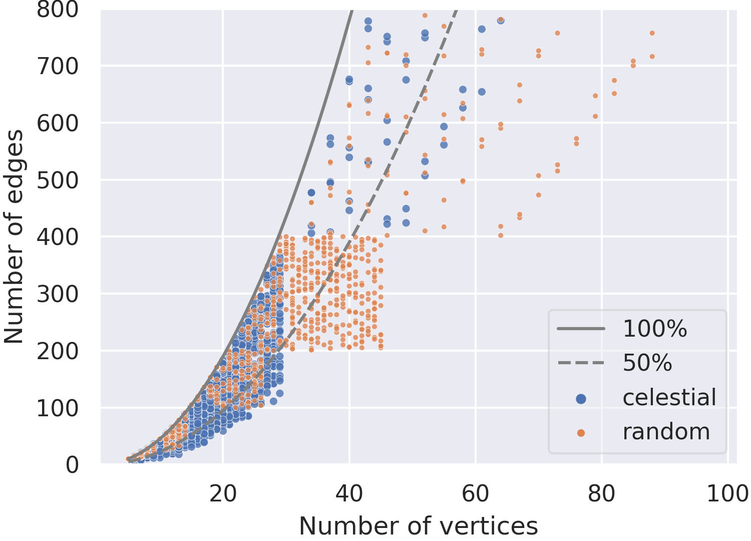
Celestial instances are inspired by real-world instances of satellites in a shared orbit, in which they maintain their relative positions while orbiting around a central body like Earth, as long as no explicit orbit-changing maneuvers are carried out. They are characterized by a set of points on a circle and a central circular obstacle. The points on the circle are chosen uniformly at random; an edge exists if and only if its vertices see each other, i.e., the edge does not intersect the central obstacle. Examples and the distribution of the nearly instances with up to edges used for our experiments can be seen in \creffig:preliminaries:instanceexamples.
All experiments were run on Intel Core i7-3770 with and of RAM.
[t].25
{subfigure}[t].45
 {subfigure}[t].25
3.1 Exact Algorithms
We developed three mixed integer programs (MIPs) and two constraint programs (CPs) to solve instances to provable optimality. Note that not every program solves all three problems. An experimental evaluation is given at the end of this section. While we focus on 2-dimensional geometric instances, all formulations are applicable to all metric cost functions.
3.1.1 Mixed Integer Program 1 (MSC-MS, MSC-TE, MSC-BE)
Our first MIP, denoted by MIP-1, uses two types of variables. The first type are real variables for all . The second type are Boolean variables for all ordered edge pairs . In a computed solution, the variables define a scan cover in which and the value of corresponds to . Because if , we directly set in these cases. Consequently, the objective functions can be expressed by substitution of with and with . Note that a - objective can be implemented by a single additional real variable and one additional constraint for each term in the objective.
We introduce a set of constraints to guarantee that the -variables and the -variables arise from a valid scan cover. Because the angle function fulfills the triangle inequality, it suffices to ensure the time difference of the -variables for all . We know that is an upper bound on the minimal makespan for a graph in 2D with vertices [14]. Moreover, a makespan of allows to scan each edge individually, and thus an optimal scan cover of MSC-BE and MSC-TE can be realized in this makespan. Therefore, by inserting the correct , we can enforce feasible scan times by using the Big-M method.
| (1) |
This leaves us with ensuring that the -variables correspond to a feasible scan cover. First, for every vertex , an incident scanned edge has at most one predecessor edge and one successor edge in the scan order.
| (2) |
Second, the total number of scanned edges at vertex is , i.e., the number of consecutively scanned edge pairs, is .
| (3) |
Together, \crefeq:ip1:hamil1,eq:ip1:hamil2 enforce that every vertex has exactly one first and one last scanned edge in the induced scan order. Because \crefeq:mip1:mtz enforces that the scan times obey the rotation times, there are no cycles in the sequence defined by if all angles are positive. This fact is very similar to the Miller-Tucker-Zemlin formulation of the TSP [23]. In the presence of -angles, we dynamically add the following constraint similar to the Dantzig formulation [12] to separate these cycles.
| (4) |
3.1.2 Mixed Integer Program 2 (MSC-MS)
The abstract definition of the MSC [14] can be directly implemented as a MIP, because absolute values can be implemented using a Boolean variable. Some modern solvers like Gurobi actually provide this functionality directly. Like for MIP-1 (\crefsec:exact:ip1), we have a real-valued variable for each that states its scan time. We try to keep the maximum value assigned to any as low as possible. For every two incident edges and , we only have the constraint that and have to be at least the time apart that needs to rotate between these two. This results in the following MIP-2.
| (5) | |||||||
| s.t. | (6) | ||||||
| (7) | |||||||
The main difference to MIP-1 is that we do not keep a record of the actually performed rotations. As a consequence, MIP-2 can only be used for MSC-MS. However, on the positive side, we do not need to dynamically add additional cycle constraints.
3.1.3 Mixed Integer Program 3 (MSC-TE, MSC-BE)
The third MIP (defined by \crefeq:ip1:hamil1,eq:ip1:hamil2,eq:ip1:dantzig,eq:ip3:globaldirectedcycle), denoted by MIP-3, is a variant of MIP-1 (\crefsec:exact:ip1) in which the -variables and the corresponding Big-M based constraint (\crefeq:mip1:mtz) are removed. As a consequence, we may use it for MSC-BE and MSC-TE, as they only need the -variables.
It is possible that the scan orders at the individual vertices are cycle free, but that the overall schedule has a deadlock when the vertices wait for each other, see \creffig:G8-2-OrderAndDepA,fig:G8-2-OrderAndDepB.
[t].3 {subfigure}[t].3
We therefore prohibit directed cycles in the scan order defined by the -variables (if not already separated by \crefeq:ip1:dantzig) dynamically via callbacks for every newly found integral solution. Violated constraints can be found via a simple DFS search.
| (8) |
Note that these cycles can also happen in MIP-1, but only with zero rotation costs between the involved edges. Thus, they are irrelevant for the solution, as all of these edges can be scanned at once.
3.1.4 Constraint Program 1 (MSC-MS)
Our first constraint program (denoted by CP-1) has the same formulation as MIP-2. The only difference between the CP version and the MIP version lies in the employed solver. In particular, absolute values can be modeled directly.
3.1.5 Constraint Program 2 (MSC-TE, MSC-BE)
Our second constraint program (defined by \crefeq:ip1:hamil1,eq:ip1:hamil2,eq:exact:cp2:mtz), denoted by CP-2, is similar to MIP-3 described in \crefsec:exact:ip3. However, MIP-3 adds \crefeq:ip1:dantzig,eq:ip3:globaldirectedcycle dynamically, which our CP does not support. Because adding all these constraints directly results in a prohibitively large formulation, we instead use a conditional variant of the Miller-Tucker-Zemlin [23] formulation to eliminate cycles in the scan order. Different from MIPs, we do not need the Big M method for CPs, but can implement conditional constraints directly. More precisely, we add the variables that state the cycle-free scan order of the edges, which is enforced by the constraints
| (9) |
3.1.6 Experimental Evaluation of Exact Algorithms
We used Gurobi (v9.0.1) for solving the MIPs and CP-SAT of Google’s or-tools (v7.7.7810) for solving the CPs. CP-SAT, which is based on a SAT solver, requires all coefficients and variables to be integral for computational efficiency. We therefore convert the floating point values to integral values including the first eight floating point digits (rounded, decimal). While this weakens the accuracy, we calculated a theoretical maximal deviation of less than , which we consider negligible and comparable to the accuracy of the MIP solver.
We considered all solvers for the three objectives on the two instance types described in the preliminaries. We evaluated how many instances of which size could still be solved to provable optimality within a time limit of ; see \creffig:engineering:exact:percentage. For MSC-MS, CP-1 has a clear lead, solving of the instances with edges for random instances, and edges for celestial instances. In our experiments, neither MIPs was able to solve any instance with more than edges to provable optimality. For MSC-TE, MIP-1 and MIP-3 performed better than CP-2, but all solvers could barely solve instances with more than edges. While MIP-1 has a more direct objective without auxiliary constraints and variables as needed for MSC-MS, its actual performance was slightly worse. For MSC-BE, CP-2 performed considerably better; for celestial instances, it can solve instances nearly twice as large ( at edges) than the MIPs. Surprisingly, MIP-1 was slightly better than CP-2 for random instances, being able to solve of the instances with edges. Overall, CPs appear to be considerably more effective than MIPs, and random instances show to be easier to solve than celestial ones.
[t].9

[t].45
 {subfigure}[t].45

3.2 Approximations and Heuristics
For larger instances (beyond the size that was solvable to provable optimality), we developed additional methods based on approximation algorithms and heuristics that provided good (but not provably optimal) solutions.
3.2.1 Bipartite Approximation Algorithms with Coloring Partition
The constant-factor approximation algorithms for bipartite graphs extend to general graphs by partitioning them into bipartite graphs and applying the corresponding approximation algorithm to each of the bipartite subgraphs. More specifically, assigning a vector over with bits to each color class of a -colored graph induces a covering of its edge set with bipartite graphs; for more details see Motwani and Naor [24]. For MSC-MS, this even preserves the approximation factor [14]. We use the well-engineered dsatur heuristic [10] for the graph coloring problem, which is shipped with the pyclustering-package [25]. Concatenating the solutions of the bipartite graphs yields a feasible scan cover; here we use a greedy approach to minimize the transition costs. We denote this method by APX.
3.2.2 (Meta-)Heuristics
We also considered a number of (meta-)heuristics for optimizing the three objectives.
- Greedy:
-
Scan the first edge regarding a given or random order and then scan the edge that increases the objective the least, until all edges are scanned. If multiple edges are equally good, the first one regarding the order is selected. Many edges can be inserted without extra cost and thus the initial edge order has a strong influence on the result.
- Iterated Local Search (ILS):
-
This simple but potentially slow heuristic considers for a given start solution (in this case of Greedy) all possible swaps of edges; the locally best swap is carried out, until no further improvement is possible.
- Simulated Annealing (SA):
-
This common variation of Iterated Local Search performs swaps according to a probability based on the Boltzmann function , where is the objective value of the current best solution, is the objective value of the considered solution, and is the current temperature. The temperature decreases over time and with it the likelihood of a worse solution being used. If the objective does not improve for some time, the temperature is increased in order to escape the local minimum. Due to randomization, we can run multiple searches in parallel. We terminate if the solution has not improved for some time.
- Genetic Algorithm (GA):
-
We start with an initial population of solutions generated by a randomized Greedy. A solution is encoded by assigning each edge a fractional number between and , similar to [19]. The scan order is determined by sorting the edges by these numbers. In each round, we build a new population by selecting the best of the old population (elitism) and then fill the rest of the population by crossovers of the old generation. For a crossover, we select two solutions of the old generation with a probability matching their objective values (uniform selection) and for each edge we choose with equal probability either the number from the first or second solution (uniform crossover). If by chance, two edges get the same number, we randomly change one of them without influencing the order. Of the new generation of solutions, are selected for mutation. A mutation applies Greedy with a probability of (the old order is used as initial edge order) or changes each edge with a probability to a new random number. This is repeated until we either reach a time limit of , generations, or generations without improvement. The best solution found during this process is then returned.
3.2.3 Experimental Evaluation of Approximations and Heuristics
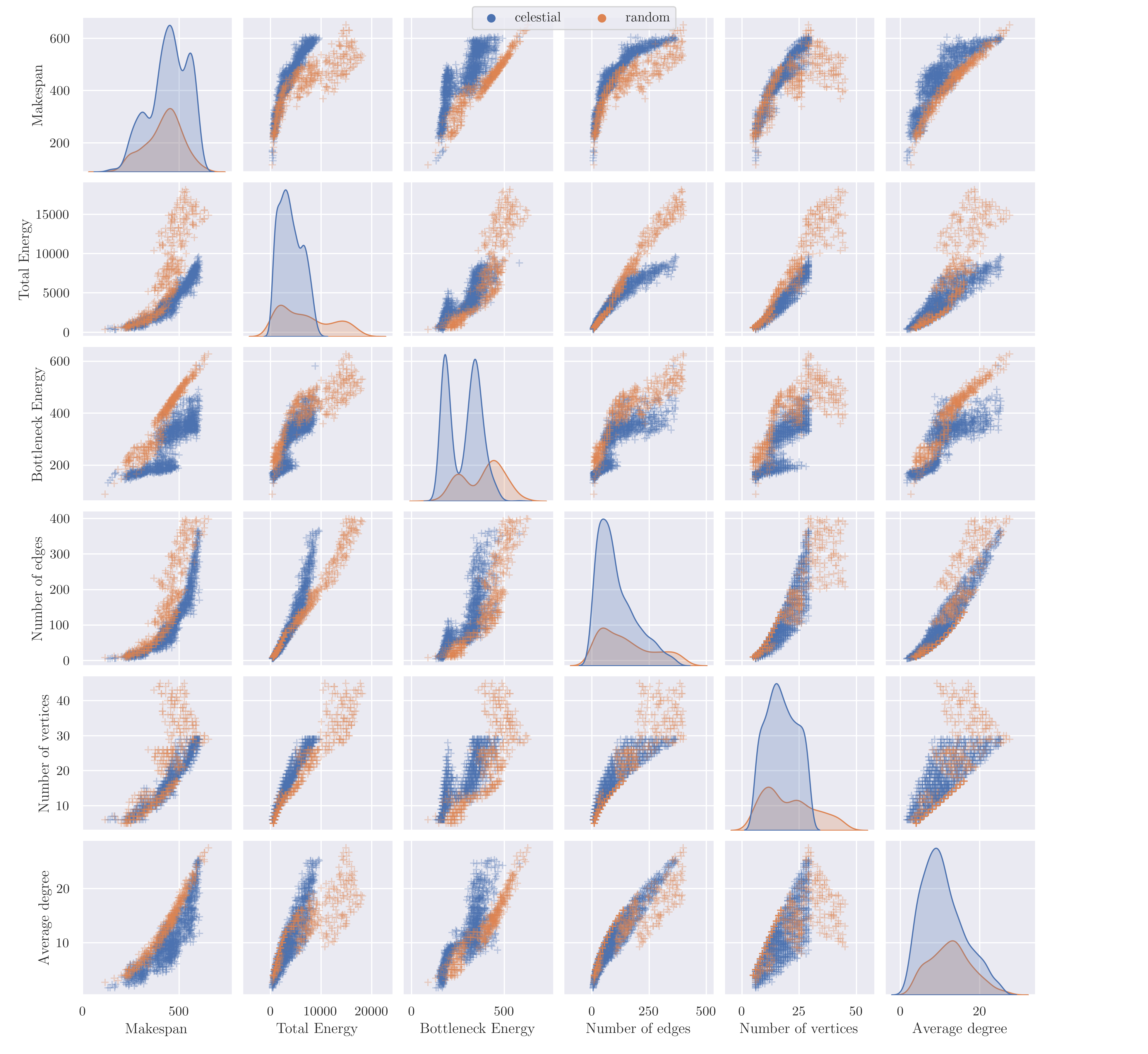
fig:engineering:inexact:overview shows experimental results for heuristically solving instances with up to edges with a time limit (at which point the current solution is returned). For MSC-MS, CP-1 yields the best results even for larger instances (where it is aborted by the time limit) by a margin of to the next best algorithm, GA. For MSC-TE, the genetic algorithm turned out to be the best approach for celestial instances by a margin of over for the larger instances. Surprisingly, CP-1 (optimizing for MSC-MS) yields slightly better solutions than the genetic algorithm for random instances of MSC-TE. The most interesting results are for MSC-BE. Here, CP-1 achieves the best results by a margin of over for random instances, and GA (TE) the best results for celestial instances by a margin of over . The excellent performance of CP-1 can be explained by a strong correlation of MSC-MS and MSC-BE for random graphs, as shown in \creffig:engineering:correlations. The fact that GA (TE) is actually better in optimizing MSC-BE than GA (BE) can be explained by the weaker gradients of bottleneck objectives, because only a small part of the solution (the most expensive vertex) actually contributes to the value. However, the initial bump, at which the exact solver of MSC-BE still yields (better) solutions, indicates that these solutions could be far from optimal and that there may still be room for improvement.
[t].96

[t].45
 {subfigure}[t].52

Overall, either CP-1 or GA (TE) yields the best solutions. CP-1 is especially strong on random instances for all three objectives. The approximation algorithm is usually among the worst. For MSC-MS, the algorithm performs a full rotation for nearly all instances, as is usually above . Note that the factor can be worse than the approximation factor (resp. ), because these are not bipartite graphs.
In \creffig:engineering:correlations (first row, fourth and last column) we can additionally see that for MSC-MS the objective correlates strongly with the number of edges for celestial instances and with the average degree for random instances. Total energy seems to primarily correlate with the number of edges for both types; our random instances are on average twice as expensive. For MSC-BE, only random graphs seem to have a significant correlation to MSC-MS and the average degree.
4 Conclusion and Open Problems
We studied problems of minimum scan cover with three different practically relevant objective functions, providing both theoretical and practical contributions: complexity and algorithmic results for the new objectives (MSC-TE and MSC-BE), and practical methods for computing provably optimal solutions for smaller and near-optimal solutions for larger instances.
In particular, we developed multiple MIP and CP formulations and demonstrated that instances of MSC-MS can be solved reliably for instances with more than edges using constraint programming which performs much better than our MIP approaches. While this approach generalizes also to 3D, we only tested 2D instances; it is open whether these results also carry over to 3D. MSC-TE and MSC-BE can only be solved to optimality for much smaller instances. For solving larger instances without guarantee of optimality, we evaluated approximation algorithms and a spectrum of meta-heuristics. Within the given time limit, CP-1 provided the best solutions for all MSC-MS instances, and even the random instances for MSC-TE and MSC-BE, despite only optimizing for MSC-MS. For celestial instances of MSC-TE and MSC-BE, the genetic algorithm optimizing for MSC-TE provides the best solutions. However, the results indicate perspectives for improving the optimization of MSC-BE.
At this point, fully dynamic instances (in which the vertices change their relative positions to each other over time, such as for satellites with different orbit parameters) are yet to be explored. These promise to be even more challenging, due to bigger gaps between optimal and suboptimal solutions, resulting from possibly long delays when a limited communication window has been missed.
References
- [1] Alok Aggarwal, Don Coppersmith, Sanjeev Khanna, Rajeev Motwani, and Baruch Schieber. The angular-metric traveling salesman problem. SIAM J. Comp., 29(3):697–711, 1999.
- [2] Ali Allahverdi. The third comprehensive survey on scheduling problems with setup times/costs. Eur. J. Oper. Res., 246(2):345–378, 2015.
- [3] Ali Allahverdi, Jatinder N.D. Gupta, and Tariq Aldowaisan. A review of scheduling research involving setup considerations. Omega, 27(2):219–239, 1999.
- [4] Ali Allahverdi, C.T. Ng, T.C. Edwin Cheng, and Mikhail Y. Kovalyov. A survey of scheduling problems with setup times or costs. Eur. J. Oper. Res., 187(3):985–1032, 2008.
- [5] Esther M. Arkin, Michael A. Bender, Erik D. Demaine, Sándor P. Fekete, Joseph S. B. Mitchell, and Saurabh Sethia. Optimal covering tours with turn costs. In Symp. Disc. Alg. (SODA), pages 138–147, 2001.
- [6] Esther M. Arkin, Michael A. Bender, Erik D. Demaine, Sándor P. Fekete, Joseph S.B. Mitchell, and Saurabh Sethia. Optimal covering tours with turn costs. SIAM J. Comp., 35(3):531–566, 2005.
- [7] Rom Aschner and Matthew J. Katz. Bounded-angle spanning tree: modeling networks with angular constraints. Algorithmica, 77(2):349–373, 2017.
- [8] Sean Augenstein, Alejandra Estanislao, Emmanuel Guere, and Sean Blaes. Optimal scheduling of a constellation of Earth-imaging satellites, for maximal data throughput and efficient human management. In Int. Conf. Automated Planning & Scheduling, pages 345–352, 2016.
- [9] Aaron T. Becker, Mustapha Debboun, Sándor P. Fekete, Dominik Krupke, and An Nguyen. Zapping Zika with a mosquito-managing drone: Computing optimal flight patterns with minimum turn cost. In Symp. Comp. Geom. (SoCG), pages 62:1–62:5, 2017.
- [10] Daniel Brélaz. New methods to color the vertices of a graph. Comm. ACM, 22(4):251–256, 1979.
- [11] Paz Carmi, Matthew J. Katz, Zvi Lotker, and Adi Rosén. Connectivity guarantees for wireless networks with directional antennas. Comp. Geom., 44(9):477–485, 2011.
- [12] George Dantzig, Ray Fulkerson, and Selmer Johnson. Solution of a large-scale traveling-salesman problem. Journal of the Op. Res. Soc. of America, 2(4):393–410, 1954.
- [13] Erik D. Demaine, Joseph S. B. Mitchell, and Joseph O’Rourke. The Open Problems Project. http://cs.smith.edu/~orourke/TOPP/.
- [14] Sándor P. Fekete, Linda Kleist, and Dominik Krupke. Minimum scan cover with angular transition costs. In Symp. Comp. Geom. (SoCG), volume 164, pages 43:1–43:18, 2020.
- [15] Sándor P. Fekete and Dominik Krupke. Covering tours and cycle covers with turn costs: Hardness and approximation. In Int. Conf. Algor. Complexity (CIAC), pages 224–236, 2019.
- [16] Sándor P. Fekete and Dominik Krupke. Practical methods for computing large covering tours and cycle covers with turn cost. In Alg. Engin. Exp. (ALENEX), pages 186–198, 2019.
- [17] Sándor P. Fekete and Gerhard J. Woeginger. Angle-restricted tours in the plane. Comp. Geom., 8:195–218, 1997.
- [18] Mike Fellows, Panos Giannopoulos, Christian Knauer, Christophe Paul, Frances A. Rosamond, Sue Whitesides, and Nathan Yu. Milling a graph with turn costs: A parameterized complexity perspective. In Worksh. Graph Theo. Conc. Comp. Sci. (WG), pages 123–134, 2010.
- [19] M. Gholami, M. Zandieh, and A. Alem-Tabriz. Scheduling hybrid flow shop with sequence-dependent setup times and machines with random breakdowns. Int. J. Adv. Manufact. Tech., 42(1-2):189–201, 2009.
- [20] Haje Korth, Michelle F. Thomsen, Karl-Heinz Glassmeier, and W. Scott Phillips. Particle tomography of the inner magnetosphere. J. Geophys. Res.: Space Phys., 107(A9):SMP–5, 2002.
- [21] Guoliang Li, Lining Xing, and Yingwu Chen. A hybrid online scheduling mechanism with revision and progressive techniques for autonomous Earth observation satellite. Acta Astronautica, 140:308–321, 2017.
- [22] László Lovász. Coverings and colorings of hypergraphs. In Southeastern Conf. Combin., Graph Th., Comput. (SEICCGTC), pages 3–12, 1973.
- [23] Clair E. Miller, Albert W. Tucker, and Richard A. Zemlin. Integer programming formulation of traveling salesman problems. J. ACM, 7(4):326–329, 1960.
- [24] Rajeev Motwani and Joseph (Seffi) Naor. On exact and approximate cut covers of graphs. Technical report, Stanford University, Stanford, CA, USA, 1994.
- [25] Andrei Novikov. PyClustering: Data mining library. J. Open Source Softw., 4(36):1230, 2019.
- [26] Thomas J. Schaefer. The complexity of satisfiability problems. In Symp. Th. Comp. (STOC), pages 216–226, 1978.
Appendix A MSC-TE and MSC-BE in 1D
In this section we present a complete proof of the following theorem.
See 1
Proof.
We assume that the vertices are placed on a horizontal line. We partition the vertices into two groups: those with a neighbor to only one side and those with neighbors to both sides. If the second group is empty, there is a trivial zero-cost solution for both objectives.
Thus, consider . Each of these vertices needs to rotate at least , so the values and are lower bounds for MSC-TE and MSC-BE, respectively. The following strategy matches this lower bound: The vertices in the first group are headed to their neighbor and do not rotate. In the following we restrict our attention to the vertices in the second group. In the beginning, all of them are headed left. Then, from left to right, one after the other rotates such that it is headed right; the next vertex starts only after the completion of its predecessor. Note that whenever a vertex rotates, all edges to its left are scanned. Consequently, this yields a valid scan cover. ∎
Appendix B NP-hardness of MSC-BE and MSC-TE
Given an instance of MNAE3SAT, we construct a graph with the same for all vertices that has a -cover if and only if is satisfiable. Recall that the Minimum Scan Cover problem with respect to the objectives MSC-BE and MSC-TE on is equivalent to finding a -cover of this graph. The choice of variable assignment is encoded by the choice of rotation direction in a -cover of specific vertices in , which we call connector vertices.
Constructing the gadgets
We construct a variable gadget (\creffig:variable-gadget) for each variable and a clause gadget (\creffig:clause-gadget) for each clause . For , we connect the gadgets and with a wire gadget (\creffig:wire-gadget). The resulting graph is symbolically shown in \creffig:hardness-construction-example. We construct both the variable gadget and wire gadget from smaller components called wire fragments , see \creffig:swap-fragment for an illustration.
We first state several observations that help with the construction of these gadgets.
Observation 7.
If an edge is the first or the last edge scanned in a -cover, it bounds a minimal -cone of vertex and of vertex .
In the gadgets, we will prescribe the two edges bounding the -cone of a vertex.
Observation 8.
Consider a straight-line drawing of a graph . For every vertex and every pair of consecutive edges at , we can add edges incident to (and new vertices of degree 1), such that in the resulting drawing, and bound the -cone of .
clm:lambdacone allows us to choose the maximal angle between consecutive edges. In the same manner, we can ensure that is equal for all vertices of the gadgets (excluding the newly added vertices of degree 1).
Next we construct the individual gadgets. Consider a wire fragment as depicted in \creffig:swap-fragment. Using \crefclm:lambdacone, we make sure that the -cones correspond to the blue arcs. The vertices can be shared between subgraphs with the following properties concerning their direction of rotation in a -cover. Note that given a -cover, we can obtain a second -cover by reversing all directions.
Lemma 9.
The vertices in the wire fragment have the following properties.
- 1.
In every -cover of , the vertices and rotate in the same direction, while rotates in the opposite direction.
- 2.
There exists a -cover of .
Proof.
Suppose we have a -cover of with scan order . Note that one of the edges , is first in , and the other last (these are the only edges bounding a minimal -cone, see Observation 7). Suppose is the first edge in . Then turns counterclockwise and turns clockwise. Additionally, turns clockwise, because is the last edge. The other case, in which is the first edge, is analogous.
The following scan order yields a -cover of in which rotates counterclockwise, see also the edge labels in Figure 24: , , , , , , , , , , , , , . ∎
[t].48 {subfigure}[t].48
For a variable , the variable gadget consists of a chain of wire fragments, as depicted in \creffig:variable-gadget. Denoting the number of occurrences of in by , we create copies of the wire fragment with vertices . Rotate the wire fragments with even index by . To combine the wire fragments, we identify the vertices and for even and the vertices and for odd . We define as the connector vertices of the variable gadget.
Lemma 10.
The variable gadget has the following properties.
- 1.
In every -cover of , all vertices in rotate in the same direction.
- 2.
There exists a -cover of .
Proof.
Suppose we have a -cover of . By \creflem:swap-properties, and rotate in the same direction, while rotates in the opposite direction. Because the wire fragments are all connected at vertices with identical properties, all copies rotate in the same direction across all wire fragments; in particular, the vertices rotate in the same direction.
For each wire fragment in , there exists a scan cover that is a -cover for the fragment (\creflem:swap-properties). Concatenating the schedules from to in this order yields a schedule for . This results in a -cover for , as vertices used in two fragments rotate in the same direction and have two -cones, one for each scan order of the two fragments. ∎
For the construction of the clause gadget of , see \creffig:clause-gadget. We place the connector vertices at the corners of an equilateral triangle, the vertices on the midpoints of the sides as illustrated, and insert the edges for all . Using \crefclm:lambdacone, we ensure that the -cones of , , and correspond to the blue arcs in the figure. Note that a small perturbation suffices to obtain rational coordinates and does not harm the construction.
Lemma 11.
The clause gadget has the following properties.
- 1.
In every -cover of , not all connector vertices in rotate in the same direction.
- 2.
For each assignment of directions to vertices in that does not assign them all the same direction, there exists a -cover of , such that every vertex in rotates in its assigned direction.
Proof.
Consider a -cover of . Note that a connector vertex turns clockwise in if and only if it scans the edge first; this edge is highlighted red in \creffig:clause-gadget.
By \crefobs:min-scan-first-last, the edges are the unique candidates for the first or last edge scanned in . Consequently, at least one connector vertex turns clockwise, and at least one turns counterclockwise.
What remains to be shown is that for all configurations of not all equal rotations, there exists a scan order that covers the minimum angle. The order , , , , , , , , is minimal and has clockwise and counterclockwise. Reversing this order is also minimal and has clockwise and counterclockwise. Up to symmetry, these are all possible configurations in which do not all rotate in the same direction. ∎
A wire gadget consists of a chain of wire fragments such that two connectors on the ends of the chain differ in angle by . Observe that the angle between the bisectors of the maximum angles of vertices and is . The construction consists of five parts that each will rotate the chain at an angle of . (We use five parts to ensure the angle is not too small, which we need for \crefcor:approximtion-hardness-2D) We connect the first four fragments, such that , , and (Figure 26). We match the bisectors of all these connections, except for the connection between and , which is . This is repeated four more times. The final part has only two wire fragments with an angle between them.
Lemma 12.
Let and be the bisectors of the outer cones of and in the wire gadget , respectively (see \creffig:wire-gadget). For any angle , the wire gadget can be constructed such that the (counterclockwise) angle between and is and fulfills the following properties.
- 1.
In every -cover of , both connector vertices and in rotate in the same direction.
- 2.
There exists a -cover of .
Proof.
By construction, the angle between the bisectors of the outer cones of and is , and the angle between the bisectors of the outer cones of and is . Therefore, the angle between the bisectors of the outer cones of and is .
Consider the order of the connector vertices of , starting at , and denote the -th vertex by . Suppose we have a -cover of . Any pair of connector vertices in the chain that belong to the same wire fragment rotates in the opposite direction (Lemma 9.1). Therefore, connector vertices with an odd number of connector vertices between them on the chain rotate in the same direction. Therefore, and rotate in the same direction.
We now give a schedule in which and rotate clockwise. By Lemma 9.2, there exists a -cover schedule relative to each wire fragment, such that rotates clockwise if and only if is odd. Concatenating the schedules from to in this order yields a schedule for . The vertices internal to the wire fragments have the same angles as in the earlier cover. Each connector vertex that is involved in one of the angles rotates in counterclockwise direction and has the angle of size inside the minimum cone, so the concatenation of the schedules covers this vertex with a minimum cone. Each connector vertex that is not involved in one of the angles has two -cones, so these vertices can be scanned in a -cover for any order of the gadgets. ∎
Finally, to construct , we first place corresponding variable and clause gadgets in the plane. We place the gadgets in a row with all clauses to the right of all variables. For a variable that occurs in a clause, we connect their gadgets by a wire gadget. To this end, we first identify a connector vertex of the variable and the connector vertex of the wire gadget . We rotate the wire such that the bisector of the -cone of in and the bisector of the outer cone of in are equal. This ensures that the identified vertex has two -cones of size (\creffig:connecting_gadgets).
By \creflem:wire-gadget we can choose the bisector of corresponding to the connector vertex of the clause. With the clauses sufficiently far to the right, we can write as linear combination of and with positive coefficients. Therefore, we can scale and to move to . As above, we get two -cones of the same size.
We are now ready to prove that MSC-TE and MSC-BE are NP-hard.
See 2
Proof.
Given an instance of MNAE3SAT, we construct with gadgets and auxiliary edges satisfying \creflem:clause-gadget,lem:variable-gadget,lem:wire-gadget. Observe that is bipartite, because all gadgets are bipartite and the identified connector vertices can all be assigned the same color. Additionally, all vertices in have the same by applying \crefclm:lambdacone. We show that is satisfiable if and only if has a -cover. Because any optimal solution to MSC-TE and MSC-BE is a -cover, if a -cover exists, this implies that both problems are NP-hard.
Suppose is satisfiable. Then there exists a variable assignment such that in no clause all values are equal. We construct a -cover for by specifying a scan order. We start with the variable gadgets. For each , scan all edges of with a -cover, as follows. If , the connector vertices rotate clockwise, otherwise counterclockwise. By \creflem:variable-gadget.2, such a scan order exists. Next, we scan all the wire gadgets such that both connector vertices of rotate in the same direction as the one attached to the vertex gadget did in the vertex gadget. By \creflem:wire-gadget, such a scan order exists. Finally, scan the clause gadgets . Each connector vertex already rotated (counter-) clockwise, depending on of the attached variable . Because is a valid (non-equal) assignment, no three connector vertices in a clause gadget rotate in the same direction. Thus, by \creflem:clause-gadget a -cover of this clause gadget exists. Therefore, all edges can be scanned by a -cover.
It remains to show the converse. Let be a -cover of . We define if rotates clockwise over its -cone, and otherwise. We claim that if is a connector vertex in gadget , yields a satisfying truth assignment to . By \creflem:variable-gadget, in any -cover of , all are equal for all connector vertices in , thus is well defined. By \creflem:wire-gadget, in any -cover, both connector vertices in gadget rotate in the same direction. Finally, by \creflem:clause-gadget, no clause gadget contains three connector vertices rotating in the same direction in a -cover. Therefore, is a valid (non-equal) assignment of , i.e., is satisfiable. Because the reduction from to can be done in time polynomial in the number of clauses and variables, this concludes the proof. ∎
See 3
Proof.
Given an instance of MNAE3SAT, consider the graph constructed in the proof of \crefthm:NP-hard-2D. Recall that by \crefclm:lambdacone, we may assume that the angle of the -cones coincide for all vertices. Define for some vertex . Let denote the minimal angle over all incident pairs of edges, for which both vertices have degree .
In a scan cover for that is not a -cover, there exists a vertex with a total rotation angle exceeding . Consequently, either scans its edges in a unidirectional rotation including the angle of size (while possibly not scanning a smaller angle ), or some angle between two edges at is covered at least twice. We may assume that both vertices of those two edges have degree , because edges with a vertex of degree can be reordered freely to get an unidirectional rotation. Therefore, this angle has size at least .
Thus the objective value of is at least , while the cost of a -cover is . Let be the ratio between these two quantities. To prove the corollary, it is sufficient to prove .
By checking all gadgets, we observe that (the angle outside the -cone of in the wire fragment, see \creffig:swap-fragment) and (which is also realized at ). The angle can be chosen smaller than any given constant by adding additional edges. This results in . ∎