Let $\{X(t),\ t\in\mathcal{T}\}$ be a $p$-dimensional vector-valued stochastic process where $\mathcal{T}$ is an interval of $\mathbb{R}$. Let $s_{1},\dots,s_{n}$ be $n$ non-overlapping locations of an observation domain $S\subset\mathbb{R}^{2}$ and $X_{1},\dots,X_{n}$ be the observations of $X$ in $s_{1},\dots,s_{n}$. Hereafter all observations are considered to be independent, which is a classical assumption in scan statistics. Spatial scan statistics aim at detecting spatial clusters and testing their significance. Hence, one tests a null hypothesis $\mathcal{H}_{0}$ (the absence of a cluster) against a composite alternative hypothesis $\mathcal{H}_{1}$ (the presence of at least one cluster $w\subset S$ presenting abnormal values of $X$).

Frévent et al. 2021 defined the notion of cluster in the univariate functional framework. Their definitions can be easily extended to the multivariate functional context by defining a multivariate magnitude cluster $w$ as follows:

where $\Delta(t)=(\Delta_{1}(t),\dots,\Delta_{p}(t))^{\top}$, all $\Delta_{i}$ are of constant and identical signs, and exists $i\in\llbracket 1;p\rrbracket$ such that $\Delta_{i}$ is non-zero over at least one sub-interval of $\mathcal{T}$. In the same way a multivariate shape cluster can be defined as follows:

where $\Delta(t)=(\Delta_{1}(t),\dots,\Delta_{p}(t))^{\top}$ and exists $i\in\llbracket 1;p\rrbracket$ such that $\Delta_{i}$ is not constant almost everywhere.

Since the article of Cressie 1977, a scan statistic is defined by the maximum of a concentration index over a set of potential clusters $\mathcal{W}$. In the following and without loss a generality, we focus on variable-size circular clusters (Kulldorff 1997, as introduced by). The set of potential clusters $\mathcal{W}$ is the set of discs centered on a location and passing through another one, with $|w|$ the number of sites in $w$:

where $w_{i,j}$ is the disc centered on $s_{i}$ that passes through $s_{j}$. Thus, a cluster cannot cover more than 50% of the studied region which is the recommended approach of Kulldorff & Nagarwalla 1995. Remark that in the literature other possibilities have been proposed such as elliptical clusters (Kulldorff et al. 2006), rectangular clusters (Chen & Glaz 2009) or graph-based clusters (Cucala et al. 2013).

We proposed a parametric scan statistic in subsection 2.2, a distribution-free one is detailed in subsection 2.3 and a new rank-based scan statistic for multivariate functional data is developed in subsection 2.4.

In this subsection the process $X$ is supposed to take values in the Hilbert space $L^{2}(\mathcal{T},\mathbb{R}^{p})$ of $p$-dimensional vector-valued square-integrable functions on $\mathcal{T}$, equipped with the inner product $\langle X,Y\rangle=\int_{\mathcal{T}}X(t)^{\top}Y(t)\ \text{d}t$.

Frévent et al. 2021 proposed a parametric scan statistic for univariate functional data based on a functional ANOVA. A multivariate version of the ANOVA is the classical MANOVA Lawley–Hotelling trace test (Oja & Randles 2004). It was adapted by Górecki & Smaga 2017 for $L^{2}(\mathcal{T},\mathbb{R}^{p})$ processes: considering two groups $g_{1}$ and $g_{2}$ of independent random observations of two $p$-dimensional stochastic processes $X_{g_{1}}$ and $X_{g_{2}}$ taking values in $L^{2}(\mathcal{T},\mathbb{R}^{p})$, it tests the equality of the two mean vector-valued functions $\mu_{g_{1}}$ and $\mu_{g_{2}}$ where $\mu_{g_{i}}(t)=\mathbb{E}[X_{g_{i}}(t)]\in\mathbb{R}^{p}$, $i=1,2,\ t\in\mathcal{T}$.

For the cluster detection problem, the null hypothesis $\mathcal{H}_{0}$ (the absence of a cluster) can be defined by $\mathcal{H}_{0}:\forall w\in\mathcal{W},\ \mu_{w}=\mu_{w^{\mathsf{c}}}=\mu_{S}$, where $\mu_{w}$, $\mu_{w^{\mathsf{c}}}$ and $\mu_{S}$ stand for the mean functions in $w$, outside $w$ and over $S$, respectively. And the alternative hypothesis $\mathcal{H}_{1}^{(w)}$ associated with a potential cluster $w$ can be defined as $\mathcal{H}_{1}^{(w)}:\mu_{w}\neq\mu_{w^{\mathsf{c}}}$. Thus we can use the functional MANOVA to compare the mean functions in $w$ and $w^{\mathsf{c}}$.
Actually Górecki & Smaga 2017 presented the adaptation of different MANOVA tests to the functional framework. However the Wilks lambda test statistic, the Lawley-Hotelling trace test statistic and the Pillai trace test statistic presented in the article showed similar performances. In addition, they often outperformed in terms of power the tests proposed in the same article that use projections. Thus we decide to study the Lawley-Hotelling trace test for the cluster detection problem by using the following statistic:

where

and

where $\bar{X}_{g}(t)=\frac{1}{|g|}\sum_{i,s_{i}\in g}X_{i}(t)$ are empirical estimators of $\mu_{g}(t)$ ($g\in\{w,w^{\mathsf{c}}\}$), $\bar{X}(t)=\frac{1}{n}\sum_{i=1}^{n}X_{i}(t)$ is the empirical estimator of $\mu_{S}(t)$.

Now, $\mathrm{LH}^{(w)}$ can be considered as a concentration index and maximized over the set of potential clusters $\mathcal{W}$, which results in the following definition of the parametric multivariate functional spatial scan statistic (PMFSS):

The potential cluster for which this maximum is obtained, namely the most likely cluster (MLC) is

We suppose that for each time $t$, $\mathbb{V}[X_{i}(t)]=\Sigma(t,t)$ for all $i\in\llbracket 1;n\rrbracket$, where $\Sigma$ is a $p\times p$ covariance matrix function.

Thus, as previously, in the context of cluster detection, the null hypothesis $\mathcal{H}_{0}$ can be defined as follows: $\mathcal{H}_{0}:\forall w\in\mathcal{W},\ \mu_{w}=\mu_{w^{\mathsf{c}}}=\mu_{S}$, where $\mu_{w}$, $\mu_{w^{\mathsf{c}}}$ and $\mu_{S}$ stand for the mean functions in $w$, outside $w$ and over $S$, respectively. And the alternative hypothesis $\mathcal{H}_{1}^{(w)}$ associated with a potential cluster $w$ can be defined as follows: $\mathcal{H}_{1}^{(w)}:\mu_{w}\neq\mu_{w^{\mathsf{c}}}$. Next, Qiu et al. 2021 proposed to compare the mean function $\mu_{w}$ in $w$ with the mean function $\mu_{w^{\mathsf{c}}}$ in $w^{\mathsf{c}}$ by using the following statistic:

where $T_{n}(t)$ is a pointwise statistic defined by the Hotelling $T^{2}$-test statistic

$\bar{X}_{w}(t)$ and $\bar{X}_{w^{\mathsf{c}}}(t)$ are the empirical estimators of the mean functions defined in subsection 2.2, and

is the pooled sample covariance matrix function.

Then $T_{n,\text{max}}^{(w)}$ is considered as a concentration index and maximized over the set of potential clusters $\mathcal{W}$, yielding to the following multivariate distribution-free functional spatial scan statistic (MDFFSS):

Without loss of generality, Oja & Randles 2004 compared the cumulative distribution functions of real multivariate observations in two groups. In the context of multivariate functional data, their statistic can be considered as a pointwise test statistic for each time $t$: the pointwise multivariate extension of the Wilcoxon rank-sum test statistic is defined as

Now we propose as previously to globalize the information over the time with

Then in the context of cluster detection, the null hypothesis is defined as $\mathcal{H}_{0}$: $\forall w\in\mathcal{W},\ \forall t,\ F_{w,t}=F_{w^{\mathsf{c}},t}$ where $F_{w,t}$ and $F_{w^{\mathsf{c}},t}$ correspond respectively to the cumulative distribution functions of $X(t)$ in $w$ and outside $w$. The alternative hypothesis $\mathcal{H}_{1}^{(w)}$ associated with a potential cluster $w$ is $\mathcal{H}_{1}^{(w)}$: $\exists t$, $F_{w,t}(x)=F_{w^{\mathsf{c}},t}(x-\Delta_{t})$, $\Delta_{t}\neq 0$.

Then $W^{(w)}$ can be considered as a concentration index and maximized over the set of potential clusters $\mathcal{W}$ so that the multivariate rank-based functional spatial scan statistic (MRBFSS) is defined as follows:

Once the most likely cluster has been detected, its significance must be evaluated. The distribution of the scan statistic $\Lambda$ ($\Lambda_{\text{PMFSS}}$, $\Lambda_{\text{MDFFSS}}$ or $\Lambda_{\text{MRBFSS}}$) is untractable under $\mathcal{H}_{0}$ due to the dependence between $\mathcal{S}^{(w)}$ and $\mathcal{S}^{(w^{\prime})}$ if $w\cap w^{\prime}\neq\emptyset$ ($\mathcal{S}=\mathrm{LH},T_{n,\text{max}}$ or $W$). Then we chose to obtain a large set of simulated datasets by randomly permuting the observations $X_{i}$ in the spatial locations. This technique called “random labelling” was already used in spatial scan statistics (Kulldorff et al. 2009; Cucala et al. 2017; Frévent et al. 2021).

Let $M$ denote the number of random permutations of the original dataset and $\Lambda^{(1)},\dots,\Lambda^{(M)}$ be the observed scan statistics on the simulated datasets. According to Dwass 1957 the p-value for $\Lambda$ observed in the real data is estimated by

Finally, the MLC is considered to be statistically significant if the associated $\hat{p}$ is less than the type I error.

Artificial datasets were generated by using the geographic locations of the 94 French départements (county-type administrative areas) as shown in Figure 6. The location of each département was defined by its administrative capital. For each artificial dataset, a spatial cluster $w$ (composed of eight départements in the Paris region ; the red area, see Figure 6 in Supplementary materials) was simulated.

The data considered is the concentration in $\mu g.m^{-3}$ of four pollutants: ozone ($\text{O}_{3}$), nitrogen dioxide ($\text{NO}_{2}$) and fine particles $\text{PM}_{10}$ and $\text{PM}_{2.5}$ corresponding respectively to particles whose diameter is less than $10\mu m$ and $2.5\mu m$. Note that the $\text{PM}_{2.5}$ particles are included in the $\text{PM}_{10}$ particles. The data provided by the French national air quality forecasting platform PREV’AIR consists in the daily average of these variables from May 1, 2020 to June 25, 2020 (56 values for each variable) aggregated at the canton (administrative subdivisions of départements) level for each of the 169 cantons of the Nord-Pas-de-Calais (a region in northern France) located by their center of gravity. The pollutants daily concentration curves in each canton are presented in Figure 4 (left panels) and the spatial distributions of the average concentrations for each pollutant over the studied time period are presented in Figure 4 (right panels).

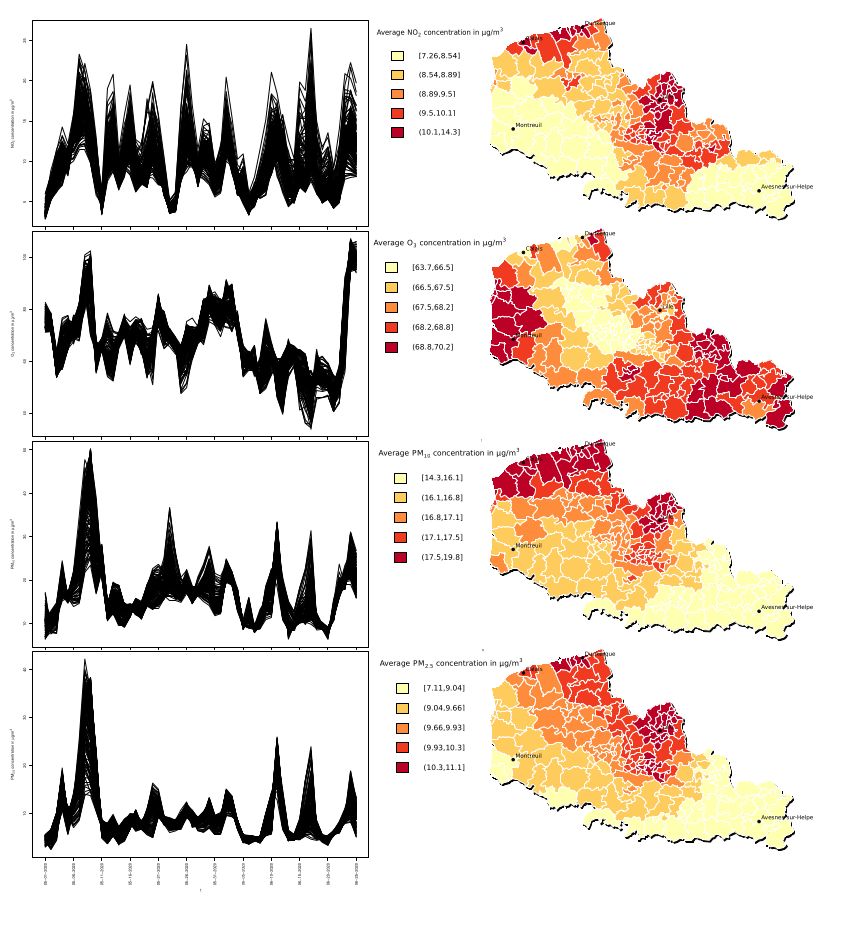
The maps in Figure 4 show a spatial heterogeneity of the average concentration for each pollutant. High concentrations of $\text{O}_{3}$ tend to aggregate in the rural areas of Montreuil and Avesnes-sur-Helpe, and high concentrations of the other pollutants tend to aggregate in the urban areas of Calais, Dunkerque and Lille. Moreover the daily concentration curves present a marked temporal variability during the period from May 1, 2020 to June 25, 2020. Thus functional spatial scan statistics seem relevant to highlight the presence of cantons-level spatial clusters of pollutants concentrations.

For the sake of concision, we have decided to present here only one method based on the results of the simulation. With regard to the latter, we have chosen the MRBFSS because it presents stable performances whatever the correlation and the distribution of the variables.

We considered a round-shaped scanning window of maximum radius 10 km since small clusters of pollution are more relevant for interpretation because the sources of the pollutants are very localized: the main source of $\text{NO}_{2}$ is road traffic, and $\text{PM}_{2.5}$ is mainly emitted in urban (heating, road traffic) or industrial areas. The statistical significance of the MLC was evaluated through 999 Monte-Carlo permutations and the MLC is said to be statistically significant if its p-value is less than 0.05. Cluster detection was also performed for the other three methods, the results are presented in Figure 8 and Table 1 in Supplementary materials.

The MRBFSS detected a significant most likely cluster (15 cantons, $308\text{km}^{2}$, $\hat{p}=0.001$) in the area of Lille. This cluster, corresponding to high values of $\text{NO}_{2}$, $\text{PM}_{10}$ and $\text{PM}_{2.5}$ concentrations, is presented in Figure 5. For these three pollutants all the curves in the MLC are above the average concentrations in the Nord-Pas-de-Calais. In environmental science it is well-known that those pollutants are more frequent in urban areas. Therefore this is consistent with the cluster observed here.

References

- Benhenni et al. (2007) Benhenni, K., Ferraty, F., Rachdi, M., & Vieu, P. (2007). Local smoothing regression with functional data. Computational Statistics, 22, 353–369. doi:10.1007/s00180-007-0045-0.
- Berrendero et al. (2011) Berrendero, J., Justel, A., & Svarc, M. (2011). Principal components for multivariate functional data. Computational Statistics & Data Analysis, 55, 2619–2634. doi:10.1016/j.csda.2011.03.011.
- Bhatt & Tiwari (2014) Bhatt, V., & Tiwari, N. (2014). A spatial scan statistic for survival data based on weibull distribution. Statistics in medicine, 33, 1867–1876.
- Boente & Fraiman (2000) Boente, G., & Fraiman, R. (2000). Kernel-based functional principal components. Statistics & Probability Letters, 48, 335–345. doi:10.1016/S0167-7152(00)00014-6.
- Chen & Glaz (2009) Chen, J., & Glaz, J. (2009). Approximations for two-dimensional variable window scan statistics. In J. Glaz, V. Pozdnyakov, & S. Wallenstein (Eds.), Scan Statistics (pp. 109 – 128). Birkhäuser Boston. doi:https://doi.org/10.1007/978-0-8176-4749-0_5.
- Chiou & Müller (2007) Chiou, J.-M., & Müller, H.-G. (2007). Diagnostics for functional regression via residual processes. Computational Statistics & Data Analysis, 15, 4849–4863. doi:10.1016/j.csda.2006.07.042.
- Chong et al. (2013) Chong, S., Nelson, M., Byun, R., Harris, L., Eastwood, J., & Jalaludin, B. (2013). Geospatial analyses to identify clusters of adverse antenatal factors for targeted interventions. International Journal of Health Geographics, 12. doi:10.1186/1476-072X-12-46.
- Cressie (1977) Cressie, N. (1977). On some properties of the scan statistic on the circle and the line. Journal of Applied Probability, 14, 272–283.
- Cucala (2014) Cucala, L. (2014). A distribution-free spatial scan statistic for marked point processes. Spatial Statistics, 10, 117–125. doi:http://dx.doi.org/10.1016/j.spasta.2014.03.004.
- Cucala et al. (2013) Cucala, L., Demattei, C., Lopes, P., & Ribeiro, A. (2013). A spatial scan statistic for case event data based on connected components. Computational Statistics, 28, 357–369. doi:https://doi.org/10.1007/s00180-012-0304-6.
- Cucala et al. (2017) Cucala, L., Genin, M., Lanier, C., & Occelli, F. (2017). A multivariate gaussian scan statistic for spatial data. Spatial Statistics, 21, 66–74. doi:10.1016/j.spasta.2017.06.001.
- Cucala et al. (2018) Cucala, L., Genin, M., Occelli, F., & Soula, J. (2018). A multivariate nonparametric scan statistic for spatial data. Spatial Statistics, 29, Pages 1–14. doi:10.1016/j.spasta.2018.10.002.
- Cuevas et al. (2002) Cuevas, A., Febrero-Bande, M., & Fraiman, R. (2002). Linear functional regression: The case of fixed design and functional response. Canadian Journal of Statistics, 30, 285–300. doi:10.2307/3315952.
- Duncan et al. (2016) Duncan, D., Rienti, M., Kulldorff, M., Aldstadt, J., Castro, M., Frounfelker, R., Williams, J., Sorensen, G., Johnson, R., Hemenway, D., & Williams, D. (2016). Local spatial clustering in youths’ use of tobacco, alcohol, and marijuana in boston. The American journal of drug and alcohol abuse, 42, 412–421. doi:10.3109/00952990.2016.1151522.
- Dwass (1957) Dwass, M. (1957). Modified randomization tests for nonparametric hypotheses. Annals of Mathematical Statistics, 28, 181–187. doi:10.1214/aoms/1177707045.
- Ferraty & Vieu (2002) Ferraty, F., & Vieu, P. (2002). Functional nonparametric model and application to sprectrometric data. Computational Statistics, 17, 545–564. doi:10.1007/s001800200126.
- Frévent et al. (2021) Frévent, C., Ahmed, M.-S., Marbac, M., & Genin, M. (2021). Detecting spatial clusters in functional data: new scan statistic approaches, .
- Gao et al. (2014) Gao, J., Zhang, Z., Hu, Y., Bian, J., Jiang, W., Wang, X., Sun, L., & Jiang, Q. (2014). Geographical distribution patterns of iodine in drinking-water and its associations with geological factors in shandong province, china. International Journal of Environmental Research and Public Health, 11, 5431–5444. doi:10.3390/ijerph110505431.
- Genin et al. (2020) Genin, M., Fumery, M., Occelli, F., Savoye, G., Pariente, B., Dauchet, L., Giovannelli, J., Vignal, C., Body-Malapel, M., Sarter, H. et al. (2020). Fine-scale geographical distribution and ecological risk factors for crohn’s disease in france (2007-2014). Alimentary Pharmacology & Therapeutics, 51, 139–148.
- Górecki & Smaga (2017) Górecki, T., & Smaga, Ł. (2017). Multivariate analysis of variance for functional data. Journal of Applied Statistics, 44, 2172–2189. doi:10.1080/02664763.2016.1247791.
- Huang et al. (2007) Huang, L., Kulldorff, M., & Gregorio, D. (2007). A spatial scan statistic for survival data. Biometrics, 63, 109–118.
- Jacques & Preda (2014) Jacques, J., & Preda, C. (2014). Model-based clustering for multivariate functional data. Computational Statistics & Data Analysis, 71, 92–106. doi:10.1016/j.csda.2012.12.004.
- Jung et al. (2007) Jung, I., Kulldorff, M., & Klassen, A. C. (2007). A spatial scan statistic for ordinal data. Statistics in medicine, 26, 1594–1607.
- Kulldorff (1997) Kulldorff, M. (1997). A spatial scan statistic. Communications in Statistics - Theory and Methods, 26, 1481–1496. doi:10.1080/03610929708831995.
- Kulldorff (1999) Kulldorff, M. (1999). Spatial scan statistics: Models, calculations, and applications. (pp. 303–322). Birkhäuser, Boston, MA. doi:10.1007/978-1-4612-1578-3_14.
- Kulldorff et al. (2009) Kulldorff, M., Huang, L., & Konty, K. (2009). A scan statistic for continuous data based on the normal probability model. Int J Health Geogr, 8. doi:https://doi.org/10.1186/1476-072X-8-58.
- Kulldorff et al. (2006) Kulldorff, M., Huang, L., Pickle, L., & Duczmal, L. (2006). An elliptic spatial scan statistic. Statistics in medicine, 25, 3929–3943. doi:10.1002/sim.2490.
- Kulldorff & Nagarwalla (1995) Kulldorff, M., & Nagarwalla, N. (1995). Spatial disease clusters: Detection and inference. Statistics in Medicine, 14, 799–810. doi:10.1002/sim.4780140809.
- Lin et al. (2016) Lin, P.-S., Kung, Y.-H., & Clayton, M. (2016). Spatial scan statistics for detection of multiple clusters with arbitrary shapes. Biometrics, 72, 1226–1234. doi:10.1111/biom.12509.
- Lin et al. (2021) Lin, Z., Lopes, M. E., & Müller, H.-G. (2021). High-dimensional manova via bootstrapping and its application to functional and sparse count data, .
- Luquero et al. (2011) Luquero, F., Banga, C., Remartínez, D., Urrutia, P. P. P., Baron, E., & Grais, R. (2011). Cholera epidemic in guinea-bissau (2008) : The importance of ”place”. PloS one, 6. doi:https://doi.org/10.1371/journal.pone.0019005.
- Martino et al. (2019) Martino, A., Ghiglietti, A., Ieva, F., & Paganoni, A. M. (2019). A k-means procedure based on a mahalanobis type distance for clustering multivariate functional data. Statistical Methods & Applications, 28, 301–322. doi:10.1007/s10260-018-00446-6.
- Oja & Randles (2004) Oja, H., & Randles, R. H. (2004). Multivariate nonparametric tests. Statistical Science, 18, 598–605. doi:10.1214/088342304000000558.
- Qiu et al. (2021) Qiu, Z., Chen, J., & Zhang, J.-T. (2021). Two-sample tests for multivariate functional data with applications. Computational Statistics & Data Analysis, 157. doi:https://doi.org/10.1016/j.csda.2020.107160.
- Ramsay & Silverman (2005) Ramsay, J., & Silverman, B. (2005). Functional Data Analysis. Springer Series in Statistics. Springer.
- Smida et al. (2020) Smida, Z., Cucala, L., & Gannoun, A. (2020). A nonparametric spatial scan statistic for functional data, .
- Tango & Takahashi (2005) Tango, T., & Takahashi, K. (2005). A flexibly shaped spatial scan statistic for detecting clusters. International Journal of Health Geographics, 4, 4–11. doi:10.1186/1476-072X-4-11.
Appendix A Supplementary materials
Figure 7 shows an example of the data generated when the are Gaussian and .