Confluent Vessel Trees with Accurate Bifurcations
Abstract
We are interested in unsupervised reconstruction of complex near-capillary vasculature with thousands of bifurcations where supervision and learning are infeasible. Unsupervised methods can use many structural constraints, e.g. topology, geometry, physics. Common techniques use variants of MST on geodesic tubular graphs minimizing symmetric pairwise costs, i.e. distances. We show limitations of such standard undirected tubular graphs producing typical errors at bifurcations where flow “directedness” is critical. We introduce a new general concept of confluence for continuous oriented curves forming vessel trees and show how to enforce it on discrete tubular graphs. While confluence is a high-order property, we present an efficient practical algorithm for reconstructing confluent vessel trees using minimum arborescence on a directed graph enforcing confluence via simple flow-extrapolating arc construction. Empirical tests on large near-capillary sub-voxel vasculature volumes demonstrate significantly improved reconstruction accuracy at bifurcations. Our code has also been made publicly available 11 1 https://vision.cs.uwaterloo.ca/code..
1 Introduction
This paper is focused on unsupervised vessel tree estimation in large volumes containing numerous near-capillary vessels and thousands of bifurcations, see Figs. 1, 10. Around of the vessels in such data have sub-voxel diameter resulting in partial volume effects such as contrast loss and gaps. Besides the topological accuracy of trees reconstructed from such challenging imagery, we are particularly interested in the accurate estimation of bifurcations due to their importance in biomedical and pharmaceutical research.
 |
 |
 |
| (a) synthetic raw data with two trees (blue & green) | (b) geodesic graph MST [13, 32, 28, 23] | (c) confluent tree reconstruction |
1.1 Unsupervised vasculature estimation methods
Unsupervised vessel tree estimation methods for complex high-resolution volumetric vasculature data combine low-level vessel filtering and algorithms for computing global tree structures based on constraints from anatomy, geometry, physics, etc. Below we review the most relevant standard methodologies.
Low-level vessel estimation: Anisotropy of tubular structures is exploited by standard vessel filtering techniques, e.g. Frangi et al. [9]. Combined with non-maximum suppression, local tubularity filters provide estimates for vessel centerline points and tangents, see \figreffig:low_level_vessels(a). Technically, elongated structures can be detected using intensity Hessian spectrum [9], optimally oriented flux models [18, 28], steerable filters [10], path operators [22] or other anisotropic models. Dense local vessel detections can be denoised using curvature regularization [24, 20]. Prior knowledge about divergence or convergence of the vessel tree (arteries vs veins) can also be exploited to estimate an oriented flow pattern [34], see \figreffig:low_level_vessels(b).

|

|
| (a) Frangi filtering [9] | (b) oriented flow pattern [34] |
Thinning: One standard approach to vessel topology estimation is via medial axis [26]. This assumes known vessel segmentation (volumetric mask) [21], which can be computed only for relatively thick vessels. Well-formulated segmentation of thin structures requires Gaussian- or min-curvature surface regularization that has no known practical algorithms. Segmentation is particularly unrealistic for sub-voxel vessels.
Geodesics and shortest paths: Geodesics [5, 2] and shortest paths [7] are often used for -interactive reconstruction of vessels between two specified points. A vessel is represented by the shortest path with respect to some anisotropic continuous (Riemannian) or discrete (graph) metric based on a local tubularity measure. Interestingly, the minimum path in an “elevated” search space combining spatial locations and radii can simultaneously estimate the vessel’s centerline and diameter, implicitly representing vessel segmentation [19, 1]. Unsupervised methods widely use geodesics as their building blocks.
Spanning trees: The standard graph concept of a minimum spanning tree (MST) is well suited for unsupervised reconstruction of large trees with unknown complex topology [13, 32, 28, 23]. MST is closely related to the shortest paths and geodesics since its optimality is defined with respect to its length. Like shortest paths, globally optimal MST can be computed very efficiently. In contrast to the shortest paths, MST can reconstruct arbitrarily complex trees without user interaction.

|

|
| (a) geodesic tubular graph | (b) MST |
The quality of MST vessel tree reconstruction depends on the underlying graph construction, see Figs. 3 and 13(a). Graphs designed for reconstructing thin tubular structures as their spanning tree (or sub-tree) are often called tubular graphs. Typically, the nodes are “anchor” points generated by low-level vessel estimators, e.g. see \figreffig:low_level_vessels. Such anchors represent sparse [29] or semi-dense [20] samples from the estimated tree structure that may be corrupted by noise and outliers. Pairwise edges on a tubular graph typically represent distances or geodesics between the nodes, as in -interactive methods discussed earlier. Such graphs are called geodesic tubular graphs, see \figreffig:tubular graph illustration.
 |
 |
 |
 | |
| image from [30] | ||||
| (a) sparse graph | (b) semi-dense geodesic tubular graphs with different size NN systems | |||
There are numerous variants of tubular graph constructions designed to represent various thin structures as MST [13, 32, 28, 23] or shortest path trees [25]. There are also interesting and useful extensions of MST addressing tubular graph outliers, e.g. k-MST [30] and integer programming technique in [29]. Such approaches are more powerful as they seek minimum sub-trees that can automatically exclude outliers. However, the corresponding optimization problems are NP-hard and require approximations. Such methods are expensive compared to the low-order polynomial complexity of MST. They are not practical for dense reconstruction problems in high-resolution vasculature volumes.
1.2 Motivation and contributions
We are interested in unsupervised reconstruction of large complex trees from vasculature volumes resolving near-capillary details. Common geodesic approaches can not represent asymmetric smoothness at bifurcations, which have forms sensitive to flow orientation. Hence, standard methods produce vessel tree reconstructions with significant bifurcation artifacts, see Figs. 1(b), 3(b) and 13(a). We define a general geometric property for oriented vessels, confluence, which is missing in prior art, and propose a practical graph-based reconstruction method enforcing it. The reconstructed confluent vessel trees have significantly better bifurcation accuracy. Our contributions are detailed below.
We introduce confluence as a geometric property for overlapping oriented smooth curves in , e.g. representing blood-flow trajectories22 2 Confluence is known in other contexts, e.g. rail tracks [15].. It is like “co-differentiability” or “co-continuity”. We define confluent vessel trees formed by overlapping oriented curves.
We extend confluence to discrete paths and trees on directed tubular graphs where directed arcs/edges represent continuous oriented arcs/curves in . We propose a simple flow-extrapolating circular arc construction that guarantees -confluence, which approximates confluence. Our confluence constraint implies directed tubular graph with asymmetric edge weights, which is in contrast to standard undirected geodesic tubular graphs [16, 13, 32, 28, 23, 30, 20, 29, 34].
We present an efficient practical algorithm for reconstructing confluent vessel trees. It uses minimum arborescence [6, 27] on our directed confluent tubular graph construction.
Our experiments on synthetic and real data confirm that confluent tree reconstruction significantly improves bifurcation accuracy. We demonstrate qualitative and quantitative improvements via standard and new accuracy measures 33 3 For our dataset and implementation of evaluation metrics discussed in this paper see https://vision.cs.uwaterloo.ca/data. evaluating tree structure, bifurcation localization, and bifurcation angles.
Our concept of confluent trees is general and our specific algorithm can be modified or extended in many ways, some of which are discussed in \secrefsec:method. To explicitly address outliers, minimum arborescence on our confluent tubular graph can be replaced by optimal sub-tree algorithms [30, 29]44 4 IP solver in [29] uses minimum arborescence as a subroutine. or explicit outlier detection [20], but these approximation algorithms address NP-hard problems and maybe too expensive for large semi-dense tubular graphs we study in this work. While outlier detection is relevant, this work is not focused on this problem.
2 Confluence of Oriented Curves
This section introduces geometrically-motivated concept of smoothness for objects containing multiple oriented curves, such as vessel trees. We define confluence as follows.
Definition 1 (confluence at a point).
Two differentiable oriented curves and are called confluent at a shared point if for some
and are s.t. , see \figreffig:confluence illustration(a).
We will call two oriented curves confluent if they are confluent at all points they share, see \figreffig:confluence illustration(b).
| (a) confluence at point | (b) confluent curves |
 |
 |
 |
| (a) | (b) | (c) |
| short confluent arc | long confluent arc | non-confluent arc |
Our concept of confluence is closely related to the geometric -continuity [4, 8]. A curve is called -continuous if at any point on the curve the slope orientation is continuous. Incidentally, the differentiability classes are too restrictive as a -continuous curve can easily be not due to the curve parameterization. Note that -continuity is only defined for a single curve while our confluence extends it for a pair of curves and can be seen as “co--continuity”.
Our concept of confluence allows defining arbitrarily complex (continuous) confluent vessel trees. Such trees are formed by multiple oriented curves representing motion trajectories of blood particles from the common root to an arbitrary number of leaves where each pair of curves must be confluent. \figreffig:confluence illustration(b) shows a simple example of a tree formed by two confluent curves with one bifurcation, which can be formally defined.
3 Confluent Tubular Graphs
Our discrete approach to reconstructing confluent vessel trees is based on efficient algorithms for directed graphs. Our “tubular” graph nodes correspond to a finite set of detected vessel points. We use discrete representation of oriented vessels as paths along directed edges or directed arcs connecting the graph nodes. Each arc on our tubular graph represents an oriented continuous “flow-extrapolating” curve in from to . Such curves could be obtained from physical models based on fluid dynamics. For simplicity, this paper is focused on oriented circular arcs, see \secrefsec:tubular_dir, motivated as the lowest-order polynomial splines capable of enforcing -continuity and confluence. In general, our confluent tubular graph construction can use higher-order flow-extrapolation models, e.g. cubic Hermite splines that are common in computer graphics and geometric modeling of motion trajectories.
By using circular arcs as flow-extrapolating curves, we introduce some ambiguity with “arcs” as the standard term for graph edges. However, this should not create confusion since there is a one-to-one relation between directed arcs on our tubular graph and the corresponding (circular) oriented arcs in . Note that both interpretations are oriented/directed. In all technically formal sentences, continuous or discrete interpretation of the “arc” is clear from the context. In more informal settings, both interpretations are often equally valid.
The rest of this Section is as follows. Oriented flow-extrapolating circular arcs between tubular graph nodes are introduced in \secrefsec:tubular_dir where -confluence constraint is defined in the context of such arcs. We also define directed arc weights to represent the confluence constraint and the local costs of sending flow along these arcs. Geometric properties of confluent circular arcs are discussed in \secrefsec:cf-cs. The algorithm estimating confluent vessel trees via minimum arborescence on our directed tubular graph is presented in \secrefsec:alg.
3.1 Confluent flow-extrapolating arcs
Formally, tubular graph is based on a set of nodes/points embedded in representing semi-densely sampled centerlines of a tubular structure. is a set of directed arcs. For our tubular graph construction, each directed arc represents some continuous oriented curve in modelling flow-extrapolation from point to point , see \figreffig:directed weights. As discussed earlier, this paper is focused on oriented circular arcs as the simplest geometric model that can represent confluent vessels, even though higher-order geometric splines or physics-motivated curves are possible. Our specific construction uses flow-extrapolating circular arcs based on a set of unit vectors representing flow direction estimates at the nodes, see Fig. 2(b). Oriented circular arc is fit into starting point , its flow orientation estimate , and the ending point , see \figreffig:directed weights. Formally, curve corresponds to a differentiable function
traversing points on a circular arc in the plane spanned by , , and vector so that
| (1) |
where derivative gives an oriented tangent.
For shortness, we define (oriented) unit tangents at the beginning and the end points of any flow-extrapolating arc as
| (2) |
The definition of arc in (1) implies so that tangent is the same for any arc starting at given point regardless of its end point . Thus,
| (3) |
where the star represents an arbitrary end point. On the other hand, tangent at the end point depends on the arc’s starting point . That is, generally,
-Confluence Constraint:
To constrain our tubular graph so that all feasible vessel trees are confluent, it suffices to enforce confluence of the arcs at the nodes where they meet. However, our simple flow-extrapolating circular arcs (1) can not be used to enforce the exact confluence. We use some threshold to introduce a relaxed version of confluence in Definition 1 for an arbitrary pair of adjacent arcs connecting points , and
In general, this is a high-order (triple clique) constraint. But, property (3) of our flow-extrapolating arc construction shows that the end point of the second arc is irrelevant. Indeed,
implying that our specific tubular graph construction allows to express confluence as a pairwise constraint
| (4) |
for any pair of points , . In essence, this becomes a constraint for our flow extrapolating arcs that can be called confluent if , see \figreffig:directed weights.
To enforce -confluence constraint, our tubular graph can simply drop all non-confluent arcs. Thus, any directed vessel tree on our graph will be confluent by construction. This paper explores the simplest approach to reconstructing confluent vessel trees as the minimum arborescence on our directed tubular graph. In this case, instead of dropping non-confluent arcs, one can incorporate -confluence constraint directly into the cost of the corresponding directed graph arcs
| (5) |
The reverse edge on our tubular graph has different weight because it corresponds to a different flow extrapolating arc that has a different length, see \figreffig:directed weights(b). As an extension, our approach also allows “elastic” arc weights by adding integral of arc’s curvature to its length in (5). It is also possible to impose soft penalties for the discrepancy between the extrapolated flow and flow estimate in (5) based on physical, physiological, or other principles.
Note that higher-order (non-circular) extrapolation arcs can be constructed to fit the flow orientation estimates at both ends exactly, implying an exactly confluent graph. However, some non-trivial physiological constraints have to be imposed on the smoothness/curvature of such (non-circular) confluent arcs which should result in very long curves in cases like \figreffig:directed weights(c). Thus, the confluence constraint will manifest itself similarly to the second line in (5).
| vessel tree reconstruction using | vessel tree reconstructions using | ||
|---|---|---|---|
| undirected Geodesic Tubular Graph (standard) | directed Confluent Tubular Graph (our) | ||
| (a) MST (blue) for Geodesic Tubular Graph (yellow) [16, 30, 34] | (b) Min Arborescence (green) for Confluent Tubular Graph (yellow) | ||
3.2 Confluence and co-circularity
Specifically for oriented circular arcs, confluence implies several interesting properties and can be juxtaposed with the standard concept of co-circularity [24]. Assume some circular flow-extrapolating arc and its reverse defined by two oriented tangents , see \secrefsec:tubular_dir and \figreffig:directed weights(a,b).
Property 1.
The angle between and is equal to the angle between and . That is,
| (6) |
While not immediately obvious, particularly in 3D, this property is not difficult to prove, see Appendix A. Identity (6) implies the following.
Theorem 1.
For circular flow extrapolating arcs, is confluent iff the reverse arc is confluent.
This theorem shows that confluence of and in \figreffig:directed weights(a,b) is not a coincidence. However, in general, such symmetry does not hold for non-circular flow-extrapolating arcs (higher order polynomial curves, etc). Also, Theorem 1 does not imply “undirectedness” of our confluent tubular graph construction using simple circular arcs. As follows from (5), since the reverse arcs and have different lengths regardless of confluence, see \figreffig:directed weights(a,b).
Interestingly, our confluence constraint in case of circular oriented arcs can be related to an “oriented” generalization of co-circularity that was originally defined in [24] for 2D curves. In co-circularity constraint can be defined for two unoriented tangent lines and at points and in a way similar to our definition of confluence for that is based on oriented tangents and . Assume unoriented circle uniquely defined in by a pair of points and tangent at the first point. If we use to denote an unoriented unit tangent of circle at any given point , then circle is uniquely defined by three conditions
| (7) |
In general, circle is different as it is defined by tangent at point , that is . Then, co-circularity constraint for and can be defined as
| (8) |
where is the angle between two lines in contrast to the angle between vectors in the similar identity (6).
The difference between confluence for , and co-circularity for , can be illustrated by the examples in \figreffig:directed weights. Note that unoriented versions of , are identical in all three examples (a,b,c) as they do not depend of the flip of orientation in (c). Thus, they are equally co-circular in (a,b,c). At the same time, oriented tangents are confluent in (a,b) while flipping orientation for results in non-confluence in (c). The properties discussed above imply that confluence can be seen as oriented generalization of co-circularity [24].
Property 2.
Confluence of oriented circular arcs or , which are defined by oriented tangents , implies co-circularity of the corresponding unoriented tangents , but not the other way around.
Note that co-circularity constraint for unoriented circular arcs along a path on a tubular graph can enforce -smoothness within a single vessel branch. But, unoriented co-circularity enforces smoothness indiscriminately in all directions from a bifurcation point without resolving conflicts between multiple branches. This leads to artifacts observed on geodesic tubular graphs, see \figreffig:gridarb(a). In contrast, the confluence constraint discriminates orientations of branches when enforcing smoothness at bifurcations, see \figreffig:gridarb(b).
3.3 Confluent tree reconstruction algorithm
Our Confluent Tree Reconstruction Algorithm 1 is discussed below. It inputs raw volumetric data with a marked root of the tree. The algorithm has four steps. First, it runs a subroutine that estimates a set of points on the tree centerline and oriented flow pattern at these points . We use a standard vector field estimation method [34] based on non-negative divergence constraint and regularization over the voxel-grid neighborhood. Since of our large vasculature volumes are near-capillary vessels, the weak sub-voxel signal often results in missing data points and grid-based regularization fails to produce consistent flow orientations, particularly at the tree periphery. We modified [34] by (anisotropically) enlarging their regularization neighborhood, see Appendix B, improving the quality of flow estimates that helps to reconstruct confluent vessel trees.
Second, we build a set of oriented arcs between the points in that correspond to directed edges on our tubular graph . Our confluence constraint works well even with a complete graph . But, for efficiency, we restrict the neighborhood to nearest neighbors (KNN). The running time is with -d trees.
The last two steps compute a directed weight for all arcs as described in \secrefsec:tubular_dir, and invoke a standard minimum arborescence algorithm that has complexity [11]. In practice, the overall running time of our method for vessel tree reconstruction is dominated by the centerline localization and flow pattern estimation in the first step.
4 Experimental results
We use two baselines which we call NMS-MST and GridMST. NMS-MST uses the Frangi method [9] along with Non-Maximum Suppression (NMS) to obtain the centerline points and local unoriented tangent estimates. On top of these, NMS-MST uses the KNN () graph of the centerline points to build the MST. Note that the KNN graph is symmetric such that a pair of nodes have an arc as long as one is a neighbor of the other. Here, the undirected edge weight is computed by the sum of two shorter arc lengths. GridMST uses [34] for estimating the centerline points and flow direction. Then, it also uses the KNN graph of the centerline points to build the MST.
GridArb uses the set of centerline points and flow estimates produced by [34], but it uses the confluent tubular graph to build the minimum arborescence (discussed in \secrefsec:alg). MArb exploits a modified version of [34] (see Appendix B) and also uses the confluent tubular graph to build the minimum arborescence. We set in (5) for all our experiments.
| Method | Flow estimates | Graph Weights | Tree Extraction |
|---|---|---|---|
| NMS-MST | Frangi et al. [9] | MST | |
| GridMST | Zhang et al. [34] | standard geodesic | |
| GridArb | Zhang et al. [34] | our confluent (5) | minimum arbores-cence |
| MArb | Modified [34], see suppl materials |
4.1 Validation Measures
Many validation measures rely on matching between the ground truth and the predicted tree. Matching algorithms could be separated into several groups. First, match the nodes of the trees independently based on a distance measure, e.g. [34, 28, 31], partial (local) sub-tree matching [12], or global tree matching approaches [17, 33, 3]. We base our evaluation approach on the first group of methods due to their efficiency and the size of our problem.
Centerline reconstruction quality. Our reconstructed tree is ideally the centerline of the vasculature. We compute the recall and fall-out statistics of the centerline points to evaluate the reconstruction quality. To obtain the centerline receiver operating characteristic (ROC) curve, we generate a sequence of recall/fall-out points by varying the detection threshold parameter for the low-level vessel filter of Frangi et al. [9].
Similarly to [34], a specific point on the ground truth centerline is considered detected correctly (recall) iff it is located within distance of a reconstructed tree where is the radius of the corresponding ground truth vessel segment and voxel-size. A point on the reconstructed tree that is farther away than this distance is considered incorrectly detected (fall-out). Before computing the ROC curve we re-sample uniformly both the ground truth and reconstructed trees.
Bifurcation reconstruction quality. We introduce two separate metrics. First, we compute the ROC curve for only bifurcation points to assess the quality of detection. Second, we measure the median angular error at the reconstructed bifurcations to assess the accuracy, where we match all ground truth bifurcations to closet branching points on the detected tree regardless of their proximity and use the median rather than the average for greater stability. The difference between our angular error measure and that in [34] is discussed in Appendix C.
|
noise std 10 |
||
|
noise std 15 |
||
| (a) centerline detection | (b) bifurcation detection |
| noise std 10 | noise std 15 |
|---|---|
4.2 Synthetic Data with Ground Truth
One of the major challenges in large-scale vessel tree reconstruction is the lack of ground truth. That complicates many interactive and supervised learning methods and makes evaluation hard. Zhang et al. [34] generated and published a dataset with ground truth using [14]. We used our newly generated 15 volumes (see Appendix D) with intensities between and . Our new dataset has a larger variance of bifurcation angles. The voxel size is mm. We add Gaussian noise with std 10 and 15.
fig:roc curves compares the results of our methods with two competitors. One is the method of [34], another baseline is simple MST computed over non-maximum suppression of vessel filter output. All methods use essentially the same detection mechanism, i.e. Frangi et al. filter, so the centerline extraction quality does not differ much. On the other hand, our method significantly outperforms in the quality of bifurcation detection, see \figreffig:roc curves (b). This result is complemented by superior angular errors in \figreffig:angular errors. We attribute this to the subvoxel accuracy and better reconstruction of bifurcation. A typical example is shown in \figreffig:teaserImages(b,c).
The GridArb performs competitively in terms of angular errors but gives the worst results in terms of centerline quality. This is due to the artifact caused by some inconsistent flow estimates near the tree periphery (see \figreffig:gridarb for concrete examples). In \secrefsec:alg we argue that enlarging the regularization neighborhood helps improve the estimation of the flow orientation.
4.3 High Resolution Microscopy CT
  |
|
 | |
 | |
 | |
 | |
 | |
 | |
   
|
 |
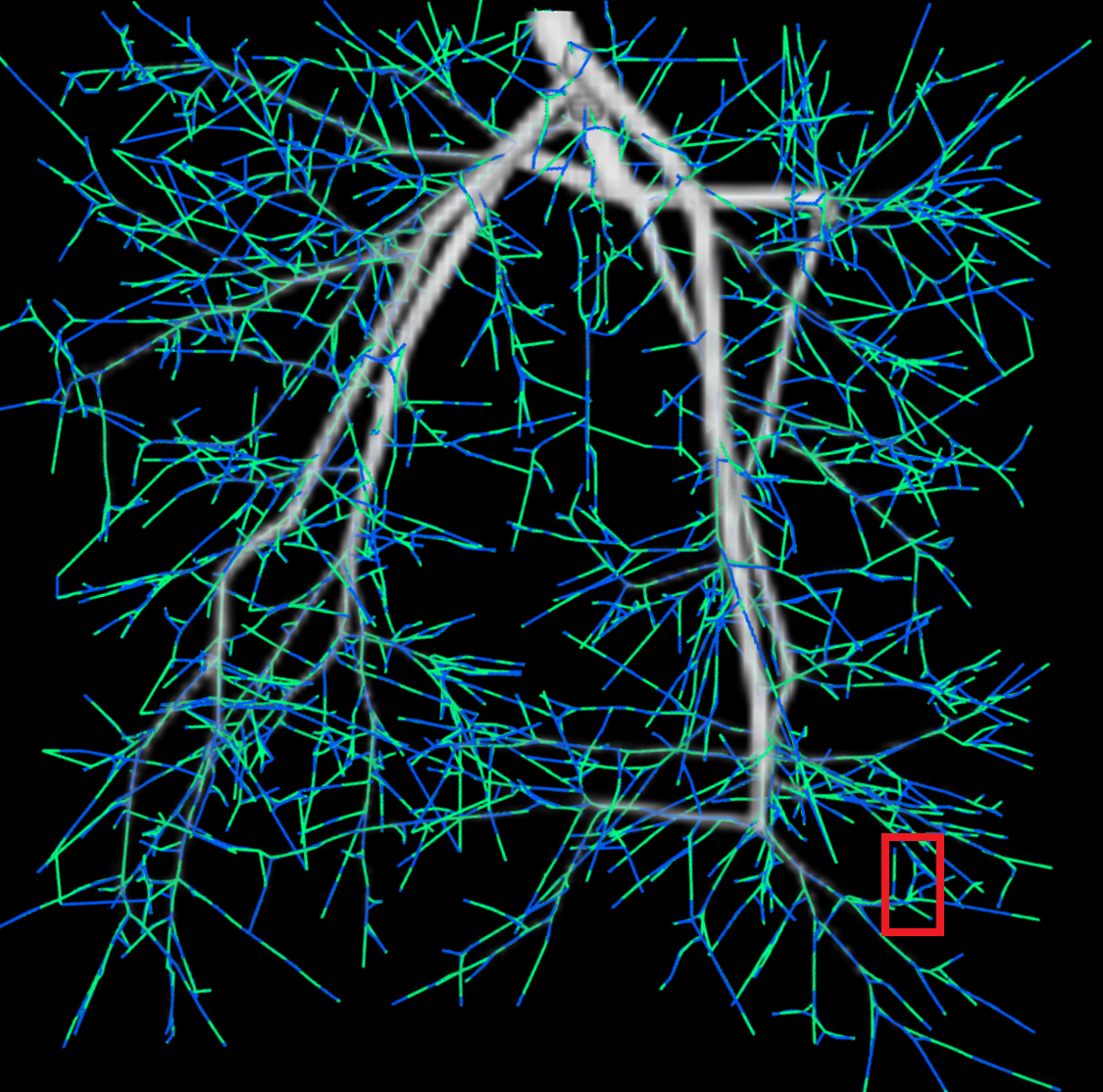
We use challenging microscopy computer tomography volume (micro-CT) of size voxels to qualitatively demonstrate the advantages of our approach. The data is a high-resolution image of mouse heart obtained ex vivo with the use of contrast. The resolution allows detecting nearly capillary level vessels, which are partially resolved (partial volume). \figreffig:real data shows the whole volume and reconstruction.
References
- [1] Fethallah Benmansour and Laurent D Cohen. Tubular structure segmentation based on minimal path method and anisotropic enhancement. IJCV, 92(2):192–210, 2011.
- [2] Da Chen, Jean-Marie Mirebeau, and Laurent D Cohen. Global minimum for a finsler elastica minimal path approach. International Journal of Computer Vision, 122(3):458–483, 2017.
- [3] Egor Chesakov. Vascular tree structure: Fast curvature regularization and validation. Electronic Thesis and Dissertation Repository. The University of Western Ontario, (3396), 2015. Master of Science thesis.
- [4] Anthony D DeRose. Geometric continuity: a parametrization independent measure of continuity for computer aided geometric design. Technical report, CA Univ Berkeley Dept of Electrical Engineering and Computer Sciences, 1985.
- [5] Thomas Deschamps and Laurent D. Cohen. Fast extraction of minimal paths in 3d images and applications to virtual endoscopy. Medical Image Analysis, 5(4):281 – 299, 2001.
- [6] Jack Edmonds. Optimum branchings. J. Res. Nat. Bur. Standards, 71B(4), October- December 1967.
- [7] M. A. T. Figueiredo and J. M. N. Leitao. A nonsmoothing approach to the estimation of vessel contours in angiograms. IEEE Transactions on Medical Imaging, 14(1):162–172, March 1995.
- [8] AH Fowler and CW Wilson. Cubic spline: A curve fitting routine. Technical report, Union Carbide Corp., Oak Ridge, Tenn. Y-12 Plant, 1966.
- [9] Alejandro F Frangi, Wiro J Niessen, Koen L Vincken, and Max A Viergever. Multiscale vessel enhancement filtering. In MICCAI’98, pages 130–137. Springer, 1998.
- [10] William T. Freeman and Edward H Adelson. The design and use of steerable filters. IEEE Transactions on Pattern Analysis & Machine Intelligence, (9):891–906, 1991.
- [11] Harold N Gabow, Zvi Galil, Thomas Spencer, and Robert E Tarjan. Efficient algorithms for finding minimum spanning trees in undirected and directed graphs. Combinatorica, 6(2):109–122, 1986.
- [12] Todd A Gillette, Kerry M Brown, and Giorgio A Ascoli. The diadem metric: comparing multiple reconstructions of the same neuron. Neuroinformatics, 9(2-3):233, 2011.
- [13] Germán González, François Fleuret, and Pascal Fua. Automated delineation of dendritic networks in noisy image stacks. In European Conference on Computer Vision, pages 214–227. Springer, 2008.
- [14] Ghassan Hamarneh and Preet Jassi. Vascusynth: simulating vascular trees for generating volumetric image data with ground-truth segmentation and tree analysis. Computerized medical imaging and graphics, 34(8):605–616, 2010.
- [15] Peter Hui, Michael J Pelsmajer, Marcus Schaefer, and Daniel Stefankovic. Train tracks and confluent drawings. Algorithmica, 47(4):465–479, 2007.
- [16] Julien Jomier, Vincent LeDigarcher, and Stephen R Aylward. Automatic vascular tree formation using the mahalanobis distance. In International Conference on Medical Image Computing and Computer-Assisted Intervention, pages 806–812. Springer, 2005.
- [17] Philip N. Klein. Computing the edit-distance between unrooted ordered trees. pages 91–102, 1998.
- [18] Max W K Law and Albert C S Chung. Three dimensional curvilinear structure detection using optimally oriented flux. In European conference on computer vision, pages 368–382. Springer, 2008.
- [19] Hua Li and Anthony Yezzi. Vessels as 4-d curves: Global minimal 4-d paths to extract 3-d tubular surfaces and centerlines. IEEE transactions on medical imaging, 26(9):1213–1223, 2007.
- [20] Dmitrii Marin, Yuchen Zhong, Maria Drangova, and Yuri Boykov. Thin structure estimation with curvature regularization. In International Conference on Computer Vision (ICCV), 2015.
- [21] Odyssée Merveille, Benoît Naegel, Hugues Talbot, and Nicolas Passat. D variational restoration of curvilinear structures with prior-based directional regularization. IEEE Transactions on Image Processing, 28(8):3848–3859, 2019.
- [22] Odyssée Merveille, Hugues Talbot, Laurent Najman, and Nicolas Passat. Curvilinear structure analysis by ranking the orientation responses of path operators. IEEE transactions on pattern analysis and machine intelligence, 40(2):304–317, 2017.
- [23] Stefano Moriconi, Maria A Zuluaga, H Rolf Jäger, Parashkev Nachev, Sébastien Ourselin, and M Jorge Cardoso. Inference of cerebrovascular topology with geodesic minimum spanning trees. IEEE transactions on medical imaging, 38(1):225–239, 2018.
- [24] Pierre Parent and Steven W Zucker. Trace inference, curvature consistency, and curve detection. PAMI, 11:823–839, 1989.
- [25] Hanchuan Peng, Fuhui Long, and Gene Myers. Automatic 3d neuron tracing using all-path pruning. Bioinformatics, 27(13):i239–i247, 2011.
- [26] Kaleem Siddiqi and Stephen Pizer. Medial representations: mathematics, algorithms and applications, volume 37. Springer Science & Business Media, 2008.
- [27] R. E. Tarjan. Finding optimum branchings. Networks, 7(1):25–35, 1977.
- [28] Engin Turetken, Carlos Becker, Przemyslaw Glowacki, Fethallah Benmansour, and Pascal Fua. Detecting irregular curvilinear structures in gray scale and color imagery using multi-directional oriented flux. In Proceedings of the IEEE International Conference on Computer Vision, pages 1553–1560, 2013.
- [29] Engin Turetken, Fethallah Benmansour, Bjoern Andres, Przemyslaw Glowacki, Hanspeter Pfister, and Pascal Fua. Reconstructing curvilinear networks using path classifiers and integer programming. IEEE Transactions on Pattern Analysis and Machine Intelligence (TPAMI), 38(12):2515–2530, December 2016.
- [30] Engin Turetken, German Gonzalez, Christian Blum, and Pascal Fua. Automated reconstruction of dendritic and axonal trees by global optimization with geometric priors. Neuroinformatics, 9(2-3):279–302, 2011.
- [31] J. A. Tyrrell, E. di Tomaso, D. Fuja, R. Tong, K. Kozak, R. K. Jain, and B. Roysam. Robust 3-d modeling of vasculature imagery using superellipsoids. IEEE Transactions on Medical Imaging, 26(2):223–237, Feb 2007.
- [32] Jun Xie, Ting Zhao, Tzumin Lee, Eugene Myers, and Hanchuan Peng. Automatic neuron tracing in volumetric microscopy images with anisotropic path searching. In International Conference on Medical Image Computing and Computer-Assisted Intervention, pages 472–479. Springer, 2010.
- [33] Kaizhong Zhang and Dennis Shasha. Simple fast algorithms for the editing distance between trees and related problems. SIAM journal on computing, 18(6):1245–1262, 1989.
- [34] Zhongwen Zhang, Dmitrii Marin, Egor Chesakov, Marc Moreno Maza, Maria Drangova, and Yuri Boykov. Divergence prior and vessel-tree reconstruction. In IEEE conference on Computer Vision and Pattern Recognition (CVPR), Long Beach, California, June 2019.
Appendix A The proof of Property 1


tree reconstruction (blue) on tree reconstructions (red and green) on undirected Tubular Graph (standard) directed Confluent Tubular Graph (our) (a) Flow pattern estimate (white) [34] (b) Flow pattern estimate (white) [34] (c) Improved flow estimate (white) + MST on geodesic tubular graph + min. arb. on confluent tubular graph + min. arb. on confluent tubular graph
Proof.
First, we only consider the circle going through , and tangential to some vector as shown in Fig. 11. Moving the tangent vector in its direction along the circle yields another tangent vector at . We also translate to . By construction, is equilateral. Thus, . Since and are tangential to the circle, we have , which obviously gives . WLOG, we assume vectors , and are all unit vectors. As , we have:
| (9) |
Now, we consider the two circles going through both and while one is tangential to and the other is tangential to the as shown in Fig. 12. Note that these two circles are not necessarily co-planar. Using (9), we can obtain
| (10) |
| (11) |
To prove (6), it is sufficient to prove equality of the two dot products which can be simplified using (10) and (11):
| (12) |
Appendix B CRF Regularization Neighborhood
Our tree extraction method is based on a directed confluent tubular graph construction presented in Sec. 3 of the paper. We proposed an approach that builds confluent flow-extrapolating arcs for our graph from estimated oriented flow vectors . Specific flow orientations can be computed from Frangi filter outputs using standard MRF/CRF regularization methods [34] enforcing divergence (or convergence) of the flow pattern. However, as mentioned in Sec. 3.3 and Sec. 4, we modified [34] by anisotropically enlarging the regularization neighborhood to improve the estimates of flow orientations, which are important for our directed arc construction. The 26-grid neighborhood regularization used in [34] generates too many CRF connectivity gaps near the vessel tree periphery where the signal gets weaker. Such gaps result in flow orientation errors, see white vectors in the zoom-ins in Fig. 13(a,b). While tree reconstruction on standard undirected geodesic tubular graphs, see Fig. 13(a), are oblivious to such errors, our directed confluent tubular graph construction is sensitive to wrong orientations, see Fig. 13(b). To address CRF gaps in the flow orientation estimator [34], we modified their 26-grid regularization neighborhood into anisotropic KNN based on Frangi’s vessel tangents [9]. This significantly reduces orientation errors in and resolves confluent tubular graph artifacts, see Fig. 13(c). We detail anisotropic KNN below.
CRF connectivity quality:
Besides the size of the neighborhood , anisotropic KNN system has another important hyper-parameter, aspect ratio . To select better parameters and , we can evaluate CRF connectivity system using ROC curves for synthetic vasculature volumes with ground truth. We consider an edge in as correct iff the projections of its ends onto the ground truth tree have parent/descendant relationship. The recall is the portion of the ground truth tree covered by the correct edges. The fall-out is the ratio of incorrect edges to the total edge count.
As shown in Fig. 14, simply increasing the size of neighborhood closes many gaps but, in the meantime, introduces a lot of spurious connections between different vessel branches. Thus, we propose to use anisotropic neighborhoods. Specifically, the regularization neighborhood is redefined as anisotropic nearest neighbors instead of regular grid connectivity. This similar to the KNN except Mahalanobis distance is used. This modification addresses the issue giving the state-of-the-art result, see Fig.13(c). To implement such anisotropic neighborhood system, we first built an isotropic KNN with some large K, eg. K=500. Then, for each node and its neighbors, we transformed the Euclidean distance into Mahalanobis distance based on the tangent direction on the node. After this, we selected K (eg. K=4) nearest neighbors for each node again based on the Mahalnobis distance. Note that such anisotropic neighborhood is symmetric since we consider a pair of nodes as neighbor as long as one is connected to the other.
Appendix C Angular Error Measure
The average angular error introduced in [34] uses only correctly detected points to compute the bifurcation angular errors. Using such matching to compare different methods is unfair as for a particular detection threshold these methods correctly detect different sets of bifurcations. So, we match all ground truth bifurcations to closet branching points on the detected tree regardless of their proximity. For certain thresholds, this causes many incorrectly matched bifurcation and large errors. Despite that such statistic is influenced significantly by random matches, it is meaningful for comparing different reconstruction methods.
Appendix D Synthetic Data with Ground Truth
Zhang et al. [34] generated and published a dataset with ground truth using [14]. We found that the diversity of bifurcation angles is limited. The mean angle is and std is . To increase the angle variance, we introduce a simple modification of vessel tree generation. When a new bifurcation is created from a point and existing line segment, we move the bifurcation towards one of the segment’s ends chosen at random decreasing the distance by half. The new mean is and std is . We generate 15 volumes with intensities between and . The voxel size is mm. We add Gaussian noise with std 10 and 15.