Cosmology beyond BAO from the 3D distribution of the Lyman-$\alpha$ forest2015Cosmology beyond BAO from the 3D distribution of the Lyman-$\alpha$ forest–References

When computing the 3D correlation function, we transform the observed redshift and angular separations $(\Delta z,\Delta\theta)$ into comoving coordinates $(r_{||},r_{\bot})$. For positions $i$ and $j$, at redshifts $z_{i}$ and $z_{j}$ and separated by an angle $\Delta\theta$, we define the radial coordinates as (du Mas des Bourboux et al. 2020)

where $D_{\mathrm{M}}(z)$ is the comoving angular diameter distance and $D_{\mathrm{C}}(z)=c\int_{0}^{z}\mathrm{d}z/H(z)$ is the radial comoving distance, with $c$ as the speed of light and $H(z)$ as the Hubble parameter. The fid term indicates that we use a fiducial cosmology to compute these distances. If the true cosmology is different from the fiducial one, the ratio between the inferred line of sight and transverse distances will be different from the true ratio. This means we will observe an apparent anisotropy in the measured correlation, which is the Alcock-Paczynski effect we wish to measure (Alcock & Paczynski 1979). Note however, that there are other sources of anisotropy, such as RSD. In order to measure the AP effect, we have to correctly model and marginalize over all other anisotropies.

When building a model for the correlation function, we follow past Ly$\alpha$ forest BAO analyses and use a template power spectrum computed using a fixed cosmology. Following Kirkby et al. 2013, we allow for small differences between the template and measured cosmologies by using general coordinate transformations of the form $r_{||}\xrightarrow{}r_{||}^{\prime}(r_{||},r_{\bot},z)$ and $r_{\bot}\xrightarrow{}r_{\bot}^{\prime}(r_{||},r_{\bot},z)$.

The most commonly used parametrisation for anisotropic re-scalings is given by:

where $(q_{||},q_{\bot})$ re-scale the coordinates along and across the line of sight respectively. However, we wish to isolate the AP effect which changes the ratio $r_{\bot}/r_{||}$. Therefore, we define the parameters:

where $\phi(z)$ re-scales the ratio: $r_{\bot}^{\prime}/r_{||}^{\prime}=\phi\;r_{\bot}/r_{||}$, and is meant to measure the AP effect. On the other hand, $\alpha(z)$ re-scales the product $r_{\bot}^{\prime}r_{||}^{\prime}=\alpha^{2}\;r_{\bot}r_{||}$, which translates into an isotropic re-scaling of $\xi$. The effect of these parameters becomes clearer when we consider their impact on the radial and transverse coordinates through small deviations around $\phi=1,\alpha=1$:

The $\alpha$ parameter produces the same effect on both $r_{||}$ and $r_{\bot}$, which corresponds to isotropic re-scaling. On the other hand, $\phi$ produces small changes that are directly opposite in $r_{||}$ versus $r_{\bot}$, which corresponds to anisotropy in $\xi$. We study the effect of these parameters on the correlation function in 2.4.

These quantities are an intermediate step between fitting the correlation function and constraining cosmological parameters. Having defined the scale parameters we will use, we turn our attention to the template and the application of these parameters.

We construct our model based on the separation of the BAO feature from the rest of the correlation. This is achieved by starting with a template isotropic linear power spectrum for an assumed fiducial cosmology, computed using CAMB (Lewis et al. 2000). This template power spectrum is decomposed into a peak (or wiggles) component, $P_{\text{peak}}(k,z_{\text{eff}})$, and a smooth (or no-wiggles) component, $P_{\text{smooth}}(k,z_{\text{eff}})$, using the method described in Kirkby et al. 2013. The reason for this separation is that BAO is a clear feature that can be used as a standard ruler; it has been studied extensively and we know that for the Ly$\alpha$ forest it is very robust when it comes to contaminants (Cuceu et al. 2020, e.g.). Therefore we consider it advantageous to separate this feature, because it will make it easier to study and understand the information contained in the rest of the correlation (i.e. in the broadband), and how it is affected by contaminants (e.g. HCDs and continuum fitting).

The full transformed correlation in the original coordinates ($r_{||},r_{\bot},z$) is given by:

where the transformed coordinates of the peak component $(r_{||}^{\prime},r_{\bot}^{\prime})$ are allowed to be different from the transformed coordinates of the smooth component $(r_{||}^{\prime\prime},r_{\bot}^{\prime\prime})$. For comparison, in BAO analyses we would fix the smooth component: $(r_{||}^{\prime\prime},r_{\bot}^{\prime\prime})=(r_{||},r_{\bot})$, whereas past full-shape analyses did not use the peak-smooth decomposition, which would be equivalent to fixing the two sets of transformations to be the same: $(r_{||}^{\prime\prime},r_{\bot}^{\prime\prime})=(r_{||}^{\prime},r_{\bot}^{\prime})$.

As we have two sets of coordinate transformations, we will need two sets of $(\phi,\alpha)$ parameters. The AP effect distorts the entire correlation, and $\phi$ is meant to measure this anisotropy. Therefore, both the smooth and peak components are affected by $\phi$ in the same way. This means that we would ideally sample only one $\phi$ parameter that re-scales both components. However, as we wish to understand the cosmological value added by re-scaling the broadband, and also study how each parameter is affected by contaminants, we will keep them separate. Going forward we will use the notation $\phi_{\mathrm{s}}$ for the smooth component and $\phi_{\mathrm{p}}$ for the BAO peak component. A measurement of $\phi$ corresponds to a measurement of:

where the AP parameter is defined as the ratio of two distances $F_{\mathrm{AP}}(z)=D_{\mathrm{M}}(z)/D_{\mathrm{H}}(z)$, with $D_{\mathrm{H}}(z)=c/H(z)$.

On the other hand, the $\alpha$ parameter has different interpretations for the peak and smooth components. We not only need to account for the different expansion histories between the template and the data, but also for the features that set the scale we measure. We denote the parameter that isotropically re-scales the peak as $\alpha_{\mathrm{p}}$ and the equivalent parameter for the smooth component as $\alpha_{\mathrm{s}}$. In the case of the BAO peak, the relevant scale is the size of the sound horizon at the end of the drag epoch, $r_{\mathrm{d}}$. The isotropic scale of the peak component, $\alpha_{\mathrm{p}}$, corresponds to a measurement of:

On the other hand, $\alpha_{\mathrm{s}}$ is harder to identify with one clear feature. The scale of matter-radiation equality ($k_{\mathrm{eq}}$) is a feature that contributes to $\alpha_{\mathrm{s}}$, and has successfully been used to constrain cosmology from the power spectrum (Baxter & Sherwin 2021; Philcox et al. 2021). However, it is not clear that it is the only feature that contributes to the isotropic scale of the broadband. Furthermore, the effect produced by $\alpha_{\mathrm{s}}$ is very similar to that of the Ly$\alpha$ flux bias, which could lead to the two parameters being hard to disentangle. Therefore, we will not focus on the cosmological interpretation of $\alpha_{\mathrm{s}}$ in this work, and leave it to future studies to determine if this parameter could be useful.

In past galaxy full-shape analyses there was no smooth/peak decomposition, and the isotropic scale parameter was interpreted using $r_{\mathrm{d}}$ (Beutler et al. 2017, e.g.). This is based on the approximation that most of the signal comes from the BAO peak. This means we can measure $\alpha_{\mathrm{p}}$ very precisely, but not $\alpha_{\mathrm{s}}$, so the measurement of a parameter $\alpha=\alpha_{\mathrm{p}}=\alpha_{\mathrm{s}}$ would be dominated by signal from the peak. By fitting two different parameters we will be able to test this assumption.

Finally, for clarity we show how our new set of parameters $(\phi_{\mathrm{s}},\alpha_{\mathrm{s}},\phi_{\mathrm{p}},\alpha_{\mathrm{p}})$ would be treated in BAO and galaxy full-shape analyses:

In the rest of this work, we show the effects of $\phi_{\mathrm{s}}$ and $\alpha_{\mathrm{s}}$ on the correlation function, study the potential for measuring them using the Ly$\alpha$ forest and its cross-correlation with quasars, and show their usefulness for constraining cosmology. However, we leave it to future work to investigate how they interact with contaminants and potential systematic errors that may affect them.

Our models for the Ly$\alpha$ forest auto-correlation and its cross-correlation with quasars follow du Mas des Bourboux et al. 2020, however we use simplified versions with no contaminants or distortion due to the effect of continuum fitting. The Ly$\alpha$ forest analyses of the auto and cross-correlation have so far only been done using models with linear-order perturbations. For Ly$\alpha\times$Ly$\alpha$, a small scale non-linear correction term is also used, with the parameter values calibrated using simulations (Arinyo-i-Prats et al. 2015). On the other hand, full-shape analyses of QSO$\times$QSO typically use higher-order perturbation theory (Taruya et al. 2010, e.g.). In this work we restrict ourselves to linear-order perturbation theory. Therefore, the full anisotropic power spectra of Ly$\alpha\times$Ly$\alpha$ ($P_{\mathrm{Ly}\alpha}$), Ly$\alpha\times$QSO ($P_{\times}$) and QSO$\times$QSO ($P_{\mathrm{QSO}}$) are given by:

where $b_{\mathrm{Ly}\alpha}$ and $b_{\mathrm{QSO}}$ are the linear biases of the Ly$\alpha$ forest and quasars respectively, $f(z)$ is the logarithmic growth rate, and $\mu_{\mathrm{k}}=k_{||}/k$, with the wavenumber $k$, and its projection along the line of sight, $k_{||}$.

The RSD parameter of the Ly$\alpha$ forest is given by:

where $b_{\eta,\mathrm{Ly}\alpha}$ is the velocity divergence bias. As $b_{\eta,\mathrm{Ly}\alpha}$ and $f(z)$ always appear together in the Ly$\alpha$ forest RSD term, they are completely degenerate. Therefore, we use the parameter $\beta_{\mathrm{Ly}\alpha}$ to define the RSD term of the Ly$\alpha$ forest, and we marginalize over it instead of $b_{\eta,\mathrm{Ly}\alpha}$. This is meant to separate the degeneracies of different parameter combinations, and to clearly differentiate between nuisance parameters ($b_{\mathrm{Ly}\alpha},b_{\mathrm{QSO}},\beta_{\mathrm{Ly}\alpha}$) and the parameters of interest ($\phi,f$). We also note that the symmetries of Equation 10 mean that when fitting only the cross-correlation, $b_{\mathrm{Ly}\alpha}$ is fully degenerate with $b_{\mathrm{QSO}}$, and similarly $\beta_{\mathrm{Ly}\alpha}$ with $f(z)/b_{\mathrm{QSO}}$.

The small-scale non-linear correction for Ly$\alpha$, $F_{\text{nl,Ly}\alpha}^{2}$, is given by the model introduced by Arinyo-i-Prats et al. 2015. However, this has only been tested and applied to the Ly$\alpha$ forest auto-correlation, and not for the cross-correlation. Therefore, we only apply this term for Ly$\alpha\times$Ly$\alpha$. On the other hand, the term $F_{\text{nl,QSO}}$, which models the quasar non-linear velocities, is used for both the cross-correlation and the quasar auto-correlation. Following Percival & White 2009, this is given by:

where $\sigma_{\mathrm{v}}$ is a free parameter representing the rms velocity dispersion.

We also model the non-linear broadening of the BAO peak by applying the term $P_{\text{nl,peak}}$ to the peak component of the power spectrum, $P_{\text{peak}}(k,z_{\text{eff}})$, following Eisenstein et al. 2007. This term is given by:

where $k_{\bot}$ is the projection of the wavenumber $k$ across the line of sight, and the smoothing scales $(\Sigma_{||},\Sigma_{\bot})$ are fixed to the values $(6.42,3.26)h^{-1}$Mpc (Kirkby et al. 2013).

We use the Vega library¹¹ 1 https://github.com/andreicuceu/vega to compute model correlation functions using the same template power spectrum (and fiducial cosmology) as in du Mas des Bourboux et al. 2020. Vega is a new, improved version of the BAO fitter in the picca²² 2 https://github.com/igmhub/picca library that was used in eBOSS Ly$\alpha$ BAO analyses.

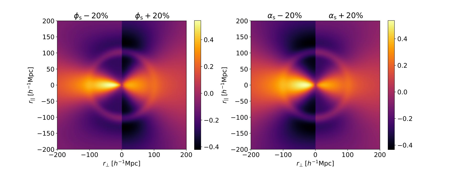
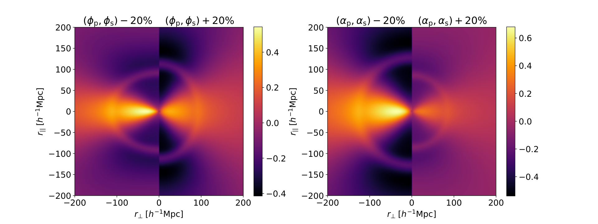
We investigate how the parameters we introduced $(\phi_{\mathrm{s}},\alpha_{\mathrm{s}},\phi_{\mathrm{p}},\alpha_{\mathrm{p}})$ change the Ly$\alpha$ forest auto-correlation function using the model presented above. We show the effect produced by these parameters in Figure 1, using contour plots of the correlation function. For each plot we show a model correlation computed using a $20\%$ smaller value of a given parameter on the left and $20\%$ higher value on the right, while the other parameters are kept fixed to one (scale parameters) or their best fit (nuisance parameters) from du Mas des Bourboux et al. 2020. Note that such changes are extreme, and chosen only to clearly showcase the effect of varying the parameters. The coordinate re-scalings we use are only approximations that work for values close to the template cosmology (parameter values around 1).

The first two rows of Figure 1 show the effect of the four parameters we introduced, with the $\phi$ parameters on the left and the isotropic scale parameters on the right. The top row shows the parameters that only affect the BAO peak, $\phi_{\mathrm{p}}$ and $\alpha_{\mathrm{p}}$, while leaving the broadband component mostly unchanged. The former produces an anisotropy in the BAO scale (top left), leading to a different position of the peak along versus across the line of sight. The latter isotropically re-scales the BAO peak (top right). On the other hand, the two plots in the middle row show the parameters that only affect the smooth component, $\phi_{\mathrm{s}}$ and $\alpha_{\mathrm{s}}$, while leaving the BAO peak unchanged. $\phi_{\mathrm{s}}$ changes the anisotropy of the smooth component (middle left). Note that $\xi$ is anisotropic even for $\phi_{\mathrm{s}}=1$ due to RSD. We will need to marginalize over this effect if we want to measure $\phi_{\mathrm{s}}$. The $\alpha_{\mathrm{s}}$ parameter isotropically re-scales the smooth component (middle right) without affecting the position of the BAO peak.

Finally, the bottom row of Figure 1 shows the effect of re-scaling the smooth and peak components at the same time by fixing $\phi_{\mathrm{s}}=\phi_{\mathrm{p}}$ (bottom left) and $\alpha_{\mathrm{s}}=\alpha_{\mathrm{p}}$ (bottom right). This means that the peak and broadband are entangled, leaving a measurement of $\alpha$ harder to interpret. This is what past full-shape analyses of discrete tracers have measured, but using different parametrisations.

We compute model correlation functions for Ly$\alpha\times$Ly$\alpha$ and Ly$\alpha\times$QSO as described in Section 2.3. The models are computed using the best fit parameter values from eBOSS DR16 ($b_{\mathrm{Ly}\alpha}$=$-0.117$, $\beta_{\mathrm{Ly}\alpha}$=$1.669$, $b_{\mathrm{QSO}}$=$3.73$, $f$=$0.97$, $\sigma_{\mathrm{v}}$=$6.86h^{-1}$Mpc), except for the scale parameters, which are all set to equal one. We use these models as our simulated data. For the purposes of this work, we wish to perform a forecast analysis, and therefore we do not add noise to the fiducial data vector.

We use covariance matrices computed from mock data sets by Farr et al. 2020. These mocks where created using the LyaCoLoRe package,³³ 3 https://github.com/igmhub/LyaCoLoRe which uses an initial Gaussian random field to simulate Ly$\alpha$ forest transmitted flux skewers and adds the relevant small scale power and RSD. The mocks were used to create full sky quasar catalogs containing $\sim 3.7$ million QSOs above redshift $z=1.8$. These simulated data products were used to compute the Ly$\alpha$ forest auto-correlation function, its cross-correlations with QSOs, the QSO auto-correlation, and the relevant covariance matrices. In order to compute a covariance matrix relevant for DESI, we use the expected DESI survey area of $14000$ square degrees, and assume it will measure roughly $\sim 1.1$ million QSOs above redshift $z=1.8$ (DESI Collaboration et al. 2016). We then compute a factor that re-scales the covariance matrix ($f_{\text{cov}}$) to match the expected DESI number density ($n_{\text{DESI}}$) and area ($A_{\text{DESI}}$):

where $n_{\text{Mock}}$ and $A_{\text{Mock}}$ are the number density and area of the mock correlation computed by Farr et al. 2020, and the factor we compute is $f_{\text{cov}}\simeq 4$. This factor is based on the fact that Ly$\alpha$ forest measurements are still limited by shot noise, and therefore the number density needs to be accounted for alongside the area, which accounts for cosmic variance. We also validate it by comparing our cosmological constraints with the forecasts from DESI Collaboration et al. 2016 in Section 3.3. The DESI simulated covariance matrix is then given by $C_{\text{DESI}}=f_{\text{cov}}C_{\text{Mock}}$, based on the mock covariance, $C_{\text{Mock}}$.

We assume that there is no cross-covariance between Ly$\alpha\times$Ly$\alpha$ and Ly$\alpha\times$QSO (du Mas des Bourboux et al. 2017), as has been standard with Ly$\alpha$ BAO analyses so far. We use a Gaussian likelihood, and compute posterior distributions using the Nested Sampler PolyChord⁴⁴ 4 https://github.com/PolyChord/PolyChordLite (Handley et al. 2015a; Handley et al. 2015b). We use the recommended setup (live_points = $25\times$ number of parameters, num_repeats = $3\times$ number of parameters) when running PolyChord. When fitting each correlation independently, we sample the parameters: $\{\phi_{\mathrm{p}},\alpha_{\mathrm{p}},\phi_{\mathrm{s}},\alpha_{\mathrm{s}},b_{\mathrm{Ly}\alpha},\beta_{\mathrm{Ly}\alpha}\}$ for the auto-correlation, while the cross-correlation has one extra parameter ($\sigma_{\mathrm{v}}$). For the cross we do not sample the QSO bias and RSD parameters due to the degeneracies with the Ly$\alpha$ parameters (see Section 2.3). When performing joint fits, we also sample $b_{\mathrm{QSO}}$ and $f(z)$; however, we treat $f(z)$ as a nuisance parameter in this section, and only focus on measuring $\phi_{s}$.

When creating our method for a two-component full-shape analysis, our first goal was to preserve the robust BAO information that we normally measure by re-scaling only the peak component. In order to check if our method succeeded in isolating this information, we fit the mock data using a BAO type model where we fix the smooth component, and only re-scale the peak. We then compare the posterior distributions of the BAO peak scale parameters ($\phi_{\mathrm{p}}$ and $\alpha_{\mathrm{p}}$) to the posteriors obtained from the full-shape analysis. The results are shown in the left panel of Figure 2. We show the constraints for a joint analysis of Ly$\alpha\times$Ly$\alpha$ and Ly$\alpha\times$QSO. We find that our method arrives at BAO measurements in very good agreement with classic BAO analyses, which means that by re-scaling the smooth component we do not influence the measurement of the position of the acoustic peak.

Our next goal for these forecasts is to understand the constraining power we have on the smooth component scale parameters, $\phi_{\mathrm{s}}$ and $\alpha_{\mathrm{s}}$. To this end, we consider a few different fitting strategies. As discussed above, before an actual measurement of these parameters, a full analysis of potential systematic errors needs to be performed. This study would inform the different analysis choices that need to be made in order to obtain robust measurements. One of these choices is the smallest scale that we fit. For past Ly$\alpha$ forest BAO analyses, this has been chosen to be $r_{\mathrm{min}}=10\;h^{-1}$Mpc. This choice is not as important for BAO analyses because the BAO peak is a large-scale feature, and so, is not affected by small-scale contaminants. However, when attempting to measure scale parameters using the broadband component, these small scales have the potential to provide a lot of information. This is both because of the extra data points, and also because these data points at small separations have higher signal-to-noise. Therefore, we test a few different values of $r_{\mathrm{min}}$ that represent the range of possible options. We showcase the best case scenario where we are not affected by systematic errors all the way down to $10\;h^{-1}$Mpc, a worst case scenario where we have to cut the small scales and $r_{\mathrm{min}}=50\;h^{-1}$Mpc, and an intermediate case where we cut to $r_{\mathrm{min}}=30\;h^{-1}$Mpc. The lower value was chosen based on the value used by Ly$\alpha$ BAO analyses, however, it might be too optimistic given current understanding of the Ly$\alpha$ correlation functions (see Section 5 for discussion). On the other hand, the choice of the upper value was made because we might start to lose BAO information when removing scales above $50\;h^{-1}$Mpc (Kirkby et al. 2013).

The forecast broadband scale parameter results (again for Ly$\alpha\times$Ly$\alpha$ and Ly$\alpha\times$QSO) are shown in the right panel of Figure 2 for different $r_{\mathrm{min}}$. Figure 2 also highlights the difference in constraining power between the AP parameter and the isotropic scale parameter. It shows that, using the BAO peak, we can obtain very good measurements of the isotropic scale parameter, $\alpha_{\mathrm{p}}$ (the $68\%$ confidence region is at a precision of $\sim 0.5\%$). However, we do not have very good constraining power when it comes to the AP parameter, $\phi_{\mathrm{p}}$, for which the $68\%$ confidence region is at a precision of $\sim 1.6\%$. This is in contrast to the AP measurement from the smooth component, where even in the worst case scenario the $68\%$ confidence region is at a precision of $\sim 0.9\%$, and in the best case scenario it is at $\sim 0.3\%$. This shows the large potential gain in cosmological information from adding this AP measurement from the broadband.

We show the benefits of extracting more information from the Ly$\alpha$ forest 3D correlation functions by performing a simple cosmological analysis using the forecast measurements obtained above. We use a flat $\Lambda$CDM model, and we first model each of the measured parameters individually, in order to understand how each of them constrains cosmology. The cosmological interpretations of the scale parameters in terms of distances are given by Equations 6 and 7. Therefore, in order to complete our model, we just need the expressions for $D_{\mathrm{M}}$ and $H(z)$ in a flat $\Lambda$CDM cosmology. The comoving angular diameter distance is given by:

and the Hubble parameter is given by the Friedmann equation:

In flat $\Lambda$CDM, the dark energy fraction can be computed from the matter and radiation fractional densities: $\Omega_{\Lambda}=1-\Omega_{\mathrm{m}}-\Omega_{\mathrm{r}}$. We also model the radiation fraction assuming a CMB temperature $T_{\mathrm{CMB}}=2.7255K$ (Fixsen et al. 1996; Fixsen 2009), and a fixed neutrino sector ⁵⁵ 5 We use $N_{\text{eff}}=3.046$, with 2 massless species and one massive with $m_{\nu}=0.06$ eV that contributes to $\Omega_{\mathrm{m}}$.. This means the only free parameters in $H(z)$ are $H_{0}$ and $\Omega_{\mathrm{m}}$.

For the AP parameter, we have a ratio of distances: $D_{\mathrm{M}}/D_{\mathrm{H}}$ (Equation 6), which means the Hubble constant cancels out. Therefore, in flat $\Lambda$CDM, $\phi$ corresponds to a measurement of $\Omega_{\mathrm{m}}$. On the other hand, for $\alpha_{\mathrm{p}}$ we have a product of distances divided by the scale of the sounds horizon squared: $D_{\mathrm{M}}D_{\mathrm{H}}/r_{\mathrm{d}}^{2}$. As each of the two distances has a factor of $1/H_{0}$, we are left with the product $H_{0}^{2}r_{\mathrm{d}}^{2}$, which means the two parameters are fully degenerate. Therefore, with $\alpha_{\mathrm{p}}$ we measure a combination of $\Omega_{\mathrm{m}}$ and the product $H_{0}r_{\mathrm{d}}$.

We use the $\alpha_{\mathrm{p}}$, $\phi_{\mathrm{p}}$ and $\phi_{\mathrm{s}}$ measurements presented above to constrain the relevant cosmological parameters. For $\phi_{\mathrm{s}}$ we use the result from the fit with $r_{\mathrm{min}}=30\;h^{-1}$Mpc, and we again use PolyChord to compute the posterior distributions. The constraints on $\alpha_{\mathrm{p}}$, $\phi_{\mathrm{p}}$ and $\phi_{\mathrm{s}}$ translate into measuring $H(z_{\mathrm{eff}})r_{\mathrm{d}}$ and $D_{\mathrm{M}}(z_{\mathrm{eff}})/r_{\mathrm{d}}$ with a precision of $\sim 0.5-0.6\%$ each. In contrast, the DESI Ly$\alpha$ BAO analysis is expected to measure $H(z_{\mathrm{eff}})r_{\mathrm{d}}$ and $D_{\mathrm{M}}(z_{\mathrm{eff}})/r_{\mathrm{d}}$ with a precision of $\sim 0.9\%$⁶⁶ 6 We recover this precision by translating the measurements of $\alpha_{\mathrm{p}}$ and $\phi_{\mathrm{p}}$ to $H(z_{\mathrm{eff}})r_{\mathrm{d}}$ and $D_{\mathrm{M}}(z_{\mathrm{eff}})/r_{\mathrm{d}}$, which validates our approach of re-scaling the covariance matrix presented in Section 3.1 (DESI Collaboration et al. 2016). The cosmological parameter results using the individual measurements and their combinations are shown in Figure 3.

The constraint from the isotropic BAO measurement ($\alpha_{\mathrm{p}}$) leads to an elongated posterior with a strong degeneracy in the $\Omega_{\mathrm{m}}-H_{0}r_{\mathrm{d}}$ space. This degeneracy is broken when combining with the $\Omega_{\mathrm{m}}$ constraint from $\phi_{\mathrm{p}}$ to obtain the usual anisotropic BAO measurement. However, as noted above, the AP measurement from the broadband is much better than the one measured from the peak. Therefore, by adding the $\phi_{\mathrm{s}}$ measurement to the BAO constraint, we can break the long correlation and obtain much better joint constraints. While the BAO measurements constrain $\Omega_{\mathrm{m}}$ and $H_{0}r_{\mathrm{d}}$ with a precision of $8.9\%$ and $3.3\%$ ($68\%$ credible regions) respectively, adding the AP measurement from the broadband improves these constraints to $2.5\%$ and $1.0\%$.

As the Ly$\alpha$ forest velocity divergence bias, $b_{\eta,\mathrm{Ly}\alpha}$, is fully degenerate with the logarithmic growth rate, $f(z)$, we have so far treated RSD as a nuisance that we need to marginalize over. In practice, RSD analyses are sensitive to the combination $f\sigma_{8}$, where $\sigma_{8}$ is the amplitude of matter perturbations in spheres of 8 Mpc/h. This means that Ly$\alpha\times$Ly$\alpha$ effectively measures the combinations $b_{\mathrm{Ly}\alpha}\sigma_{8}$ and $b_{\eta,\mathrm{Ly}\alpha}f\sigma_{8}$.

The Ly$\alpha$-QSO cross-correlation could in theory be used to measure $f\sigma_{8}$. However, on its own it cannot constrain all the biases $(b_{\mathrm{Ly}\alpha},b_{\eta,\mathrm{Ly}\alpha},b_{\mathrm{QSO}})$ even for BAO analyses where we fix $f\sigma_{8}$ (du Mas des Bourboux et al. 2020, see Section 2.3 and). On the other hand, a joint full-shape analysis of Ly$\alpha\times$QSO and Ly$\alpha\times$Ly$\alpha$ could help break these degeneracies and produce an $f\sigma_{8}$ constraint.

Another option for measuring $f\sigma_{8}$ at high redshift $(1.8<z<4)$ is to use the quasar auto-correlation, QSO$\times$QSO. The growth rate of structure was first measured from the quasar distribution by the eBOSS collaboration using the SDSS DR14 data (Gil-Marín et al. 2018; Zarrouk et al. 2018; Hou et al. 2018). They performed full-shape analyses on both the 3D power spectrum and the 3D correlation function. With the last eBOSS analysis using SDSS DR16, these measurements have been updated and now provide a $\sim 10\%$ constraint on the growth rate at an effective redshift $z_{\mathrm{eff}}=1.48$ (Hou et al. 2020; Neveux et al. 2020). The QSO sample contained $343,708$ quasars and spanned a redshift range of $0.8<z<2.2$. For comparison, DESI will measure about $1.7$ million QSOs at $z<2.1$ to be used as tracers only, and another $0.7$ million at $z>2.1$ to be used both as tracers and to measure the Ly$\alpha$ forest (DESI Collaboration et al. 2016).

The high redshift QSO$\times$QSO measurement could be combined with the two Ly$\alpha$ forest correlations in a joint analysis. This could lead to improved $f\sigma_{8}$ constraints because of the information from the cross-correlation, and also due to the potential of the three correlations helping break parameter degeneracies. Therefore, our goal in this section is to study the potential of a high-redshift joint analysis of the three two-point (high-$z$ $3\times 2$pt) correlation functions: Ly$\alpha\times$Ly$\alpha$, Ly$\alpha\times$QSO and QSO$\times$QSO.

We use a template linear power spectrum with a fixed normalization, which is proportional to $\sigma_{8}$. The logarithmic growth rate, $f(z)$, and $\sigma_{8}$ are completely degenerate in linear theory (Percival & White 2009), and therefore we are sensitive to the product $f(z)\sigma_{8}(z)$ for quasars and $b_{\eta,\mathrm{Ly}\alpha}f(z)\sigma_{8}(z)$ for the Ly$\alpha$ forest. As $b_{\eta,\mathrm{Ly}\alpha}$ is unknown, we will continue sampling over the $\beta_{\mathrm{Ly}\alpha}$ parameter, effectively treating the Ly$\alpha$ forest RSD term as a nuisance to be marginalized over.

We perform our analysis of the high-$z$ $3\times 2$pt using the two-component full-shape method we introduced in Section 2. For the Ly$\alpha$ forest auto and cross correlation we use the same simulated data and covariance matrices as described in Section 3. For the QSO auto-correlation we also use a covariance matrix computed by Farr et al. 2020, re-scaled to the DESI area and number density as described in 3.1. The QSO$\times$QSO simulated correlation function is given by a fiducial model (no noise) following the best fit parameter values from du Mas des Bourboux et al. 2020, again with the scale parameters set to unity.

Our effective parameter vector for joint fits is given by: $\{\phi_{\mathrm{p}},\alpha_{\mathrm{p}},\phi_{\mathrm{s}},\alpha_{\mathrm{s}},f\sigma_{8},b_{\mathrm{Ly}\alpha}\sigma_{8},b_{\mathrm{QSO}}\sigma_{8},\beta_{\mathrm{Ly}\alpha},\sigma_{\mathrm{v}}\}$. When fitting individual correlations we follow the approach we took in Section 3, of fixing the QSO bias and RSD terms for the cross-correlation.

In our parametrisation, the BAO parameters $(\phi_{\mathrm{p}},\alpha_{\mathrm{p}})$ are decoupled from the rest of the analysis. Therefore, as long as there is negligible cross-covariance between the different correlations, there is no benefit to $(\phi_{\mathrm{p}},\alpha_{\mathrm{p}})$ constraints from performing a joint analysis (i.e. fitting the correlations as one data vector). This has been the case so far with Ly$\alpha\times$Ly$\alpha$ and Ly$\alpha\times$QSO in BOSS and eBOSS (Bautista et al. 2017; du Mas des Bourboux et al. 2017; du Mas des Bourboux et al. 2020, e.g.), but the cross-covariance for DESI remains to be studied.

The benefits of performing the joint analysis should be most pronounced when it comes to the parameters we measure from the full-shape analysis: $\phi_{\mathrm{s}}$, $\alpha_{\mathrm{s}}$ and $f\sigma_{8}$. This is firstly due to the fact that these parameters are correlated with some of the nuisance parameters, and therefore, a joint analysis would allow us to disentangle their effects and lead to improved constraints. This is illustrated in Figure 4 (where we use a minimum separation $r_{\mathrm{min}}=30\;h^{-1}$Mpc). The top two rows show parameters that are only measured by the Ly$\alpha$ auto-correlation, while the bottom two rows show parameters that are only measured by the QSO auto-correlation. Note that the fact that $\phi_{\mathrm{s}}$ does not seem to be correlated with $b_{\eta,\mathrm{Ly}\alpha}f\sigma_{8}$ in Figure 4 for Ly$\alpha\times$Ly$\alpha$ is just due to the scale of the axes which is set to display the weak QSO$\times$QSO constraint. AP and RSD are correlated, however, we do not expect these correlations to be the same for galaxies and the forest because the two tracers cluster differently (e.g. $\beta_{\mathrm{Ly}\alpha}\sim 1.67$ while $\beta_{\mathrm{QSO}}\equiv f/b_{\mathrm{QSO}}\sim 0.26$).

The cross-correlation requires all four parameters: $(b_{\mathrm{Ly}\alpha}\sigma_{8},b_{\eta,\mathrm{Ly}\alpha}f\sigma_{8},b_{\mathrm{QSO}}\sigma_{8},f\sigma_{8})$, however, the system is degenerate. On the other hand, when we run a joint analysis of the cross-correlation with the Ly$\alpha$ auto-correlation (blue) we are able to constrain this system, because of the tight measurements of $b_{\mathrm{Ly}\alpha}\sigma_{8}$ and $b_{\eta,\mathrm{Ly}\alpha}f\sigma_{8}$ from Ly$\alpha\times$Ly$\alpha$. This leads to a constraint on $f\sigma_{8}$ of $12.8\%$ ($68\%$ confidence region), which is tighter than the one from the QSO auto-correlation of $15.4\%$ (bottom left panel of Figure 4).

The second benefit of performing this joint analysis is due to the correlation between RSD and the AP effect. When measuring $f\sigma_{8}$, we have to marginalize over the AP parameter. If we knew the true background cosmology, i.e. for fixed AP, we would obtain much better measurements of the growth rate. Even though the Ly$\alpha$ auto cannot directly measure the growth rate, it constrains the AP parameters (especially $\phi_{\mathrm{s}}$) very precisely. Therefore, including Ly$\alpha\times$Ly$\alpha$ in a joint analysis with QSO$\times$QSO can help break the correlation between RSD and AP, and improve the $f\sigma_{8}$ constraint. This is illustrated in the bottom left panel of Figure 4.

The joint high-$z$ $3\times 2$pt analysis appears to work well in breaking parameter correlations when it comes to $f\sigma_{8}$ and $\phi_{\mathrm{s}}$. However, that is not the case with $\alpha_{\mathrm{s}}$. While performing a joint analysis does lead to better constraints on this parameter, the posterior remains very correlated with all three biases (right column of Figure 4). This leaves a measurement of $\alpha_{\mathrm{s}}$ prone to systematic errors, and therefore supports our decision from Section 2 not to focus on its cosmological interpretation.

So far in this section we used a minimum separation of $r_{\text{min}}=30\;h^{-1}$Mpc to show how joint analyses help us break parameter degeneracies. However, we also want to test how these potential $f\sigma_{8}$ measurements would be affected if we could go to smaller scales (e.g. by having better models for non-linearities), or we had to cut even more data due to systematic effects on these scales. We show this in Figure 5, where we plot the marginalized fractional $68\%$ credible regions on $f\sigma_{8}$ from the QSO auto, the Ly$\alpha$ auto $+$ cross, and the joint analysis of all three correlations. We find that when we can include data at small scales ($r_{\text{min}}\lesssim 35\;h^{-1}$Mpc), the Ly$\alpha$ auto $+$ cross combination (blue line) gives us better constraints compared to the QSO auto (black line). On the other hand, if we have to cut the small scales ($r_{\text{min}}\gtrsim 35\;h^{-1}$Mpc), the Ly$\alpha$ measurement degrades very fast, and the QSO auto becomes comparable and even slightly better at constraining $f\sigma_{8}$. This gives another advantage for performing a joint high-$z$ $3\times 2$pt analysis, because it leads to much more stable and robust measurements (red line). While the quasar auto-correlation can constrain $f\sigma_{8}(z_{\mathrm{eff}}\simeq 2.3)$ with a precision of $12-20\%$ depending on $r_{\mathrm{min}}$, the high-$z$ $3\times 2$pt analysis can achieve a precision of $5-12\%$.

We have also checked how the two-component full-shape approach affects our results by comparing it with the approach usually taken in galaxy full-shape analyses of fitting the full correlation as one component (no peak/smooth decomposition). The $f\sigma_{8}$ constraints are larger when sampling four parameters (our two-component approach) versus two parameters (the one-component approach used in galaxy full-shape analyses). This is to be expected as the model has more degrees of freedom. However, the effect is very small when it comes to the high-$z$ $3\times 2$pt constraints. We found that using a value of $r_{\text{min}}=30\;h^{-1}$Mpc, we obtain a precision of $7.9\%$ on $f\sigma_{8}$ with the two-component approach, while with the one-component approach we obtain a precision of $7.6\%$. This does not significantly affect our conclusions in this work, but the two-component approach might be more advantageous when the effects of contaminants are studied, as it decouples the peak from the broadband (see Section 5).

Finally, in Figure 6 we emphasize how useful a full-shape high-$z$ $3\times 2$pt analysis would be. We show in blue some of the current $f\sigma_{8}$ measurements from different surveys (Ross et al. 2015; Alam et al. 2017; eBOSS Collaboration et al. 2020; Beutler et al. 2011; Blake et al. 2012; Okumura et al. 2016; Pezzotta et al. 2017). All of these measurements are at redshifts $z<2$, with most of them at $z<1$. The three points on the right show our DESI forecasts of $f\sigma_{8}(z_{\mathrm{eff}})$ at an effective redshift $z_{\mathrm{eff}}\simeq 2.3$. We use a conservative $r_{\mathrm{min}}=30\;h^{-1}$Mpc. This analysis would allow us to study the growth rate of cosmic structures at higher redshifts than ever before.

The results in this section show the potential of a joint full-shape analysis of the three correlation functions: Ly$\alpha\times$Ly$\alpha$, Ly$\alpha\times$QSO and QSO$\times$QSO, when it comes to measuring RSD and the AP effect. The next steps required for such an analysis are to improve the model by adding contaminants and better non-linear models, and to study the potential systematic errors that would affect this measurement, especially on the Ly$\alpha$ forest side where a full-shape analysis of the 3D correlation function has never been done. We discuss these in more detail in the next section.

References

- Alam et al. (2017) Alam S., et al., 2017, MNRAS, 470, 2617
- Alcock & Paczynski (1979) Alcock C., Paczynski B., 1979, Nature, 281, 358
- Arinyo-i-Prats et al. (2015) Arinyo-i-Prats A., Miralda-Escudé J., Viel M., Cen R., 2015, J. Cosmology Astropart. Phys., 2015, 017
- Ata et al. (2018) Ata M., et al., 2018, MNRAS, 473, 4773
- Bautista et al. (2017) Bautista J. E., et al., 2017, A&A, 603, A12
- Baxter & Sherwin (2021) Baxter E. J., Sherwin B. D., 2021, MNRAS, 501, 1823
- Beutler et al. (2011) Beutler F., et al., 2011, MNRAS, 416, 3017
- Beutler et al. (2012) Beutler F., et al., 2012, MNRAS, 423, 3430
- Beutler et al. (2017) Beutler F., et al., 2017, MNRAS, 466, 2242
- Blake et al. (2011) Blake C., et al., 2011, MNRAS, 415, 2876
- Blake et al. (2012) Blake C., et al., 2012, MNRAS, 425, 405
- Blomqvist et al. (2019) Blomqvist M., et al., 2019, A&A, 629, A86
- Busca et al. (2013) Busca N. G., et al., 2013, A&A, 552, A96
- Chen et al. (2021) Chen S.-F., Vlah Z., White M., 2021, arXiv e-prints, p. arXiv:2103.13498
- Cole et al. (2005) Cole S., et al., 2005, MNRAS, 362, 505
- Croft et al. (1999) Croft R. A., Weinberg D. H., Pettini M., Hernquist L., Katz N., 1999, The Astrophysical Journal, 520, 1
- Croft et al. (2002) Croft R. A., Weinberg D. H., Bolte M., Burles S., Hernquist L., Katz N., Kirkman D., Tytler D., 2002, The Astrophysical Journal, 581, 20
- Cuceu et al. (2020) Cuceu A., Font-Ribera A., Joachimi B., 2020, J. Cosmology Astropart. Phys., 2020, 035
- DESI Collaboration et al. (2016) DESI Collaboration et al., 2016, arXiv e-prints, p. arXiv:1611.00036
- Eisenstein et al. (2005) Eisenstein D. J., et al., 2005, ApJ, 633, 560
- Eisenstein et al. (2007) Eisenstein D. J., Seo H.-J., White M., 2007, ApJ, 664, 660
- Farr et al. (2020) Farr J., et al., 2020, J. Cosmology Astropart. Phys., 2020, 068
- Fixsen (2009) Fixsen D. J., 2009, ApJ, 707, 916
- Fixsen et al. (1996) Fixsen D. J., Cheng E. S., Gales J. M., Mather J. C., Shafer R. A., Wright E. L., 1996, ApJ, 473, 576
- Font-Ribera & Miralda-Escudé (2012) Font-Ribera A., Miralda-Escudé J., 2012, J. Cosmology Astropart. Phys., 2012, 028
- Font-Ribera et al. (2013) Font-Ribera A., et al., 2013, J. Cosmology Astropart. Phys., 2013, 018
- Font-Ribera et al. (2014) Font-Ribera A., et al., 2014, Journal of Cosmology and Astro-Particle Physics, 2014, 027
- Gil-Marín et al. (2018) Gil-Marín H., et al., 2018, MNRAS, 477, 1604
- Givans & Hirata (2020) Givans J. J., Hirata C. M., 2020, Phys. Rev. D , 102, 023515
- Handley et al. (2015a) Handley W. J., Hobson M. P., Lasenby A. N., 2015a, MNRAS, 450, L61
- Handley et al. (2015b) Handley W. J., Hobson M. P., Lasenby A. N., 2015b, MNRAS, 453, 4384
- Hou et al. (2018) Hou J., et al., 2018, MNRAS, 480, 2521
- Hou et al. (2020) Hou J., et al., 2020, MNRAS, 500, 1201
- Hui et al. (1999) Hui L., Stebbins A., Burles S., 1999, ApJ, 511, L5
- Kirkby et al. (2013) Kirkby D., et al., 2013, J. Cosmology Astropart. Phys., 2013, 024
- Lewis et al. (2000) Lewis A., Challinor A., Lasenby A., 2000, ApJ, 538, 473
- Lynds (1971) Lynds R., 1971, The Astrophysical Journal, 164, L73
- McDonald (2003) McDonald P., 2003, ApJ, 585, 34
- McDonald & Miralda-Escudé (1999) McDonald P., Miralda-Escudé J., 1999, ApJ, 518, 24
- McDonald et al. (2000) McDonald P., Miralda-Escude J., Rauch M., Sargent W. L., Barlow T. A., Cen R., Ostriker J. P., 2000, The Astrophysical Journal, 543, 1
- Neveux et al. (2020) Neveux R., et al., 2020, MNRAS, 499, 210
- Okumura et al. (2016) Okumura T., et al., 2016, PASJ, 68, 38
- Percival & White (2009) Percival W. J., White M., 2009, MNRAS, 393, 297
- Pezzotta et al. (2017) Pezzotta A., et al., 2017, A&A, 604, A33
- Philcox et al. (2021) Philcox O. H. E., Sherwin B. D., Farren G. S., Baxter E. J., 2021, Phys. Rev. D , 103, 023538
- Planck Collaboration et al. (2020) Planck Collaboration et al., 2020, A&A, 641, A6
- Rauch (1998) Rauch M., 1998, Annual Review of Astronomy and Astrophysics, 36, 267
- Reid et al. (2012) Reid B. A., et al., 2012, MNRAS, 426, 2719
- Rogers et al. (2018) Rogers K. K., Bird S., Peiris H. V., Pontzen A., Font-Ribera A., Leistedt B., 2018, MNRAS, 476, 3716
- Ross et al. (2015) Ross A. J., Samushia L., Howlett C., Percival W. J., Burden A., Manera M., 2015, MNRAS, 449, 835
- Samushia et al. (2014) Samushia L., et al., 2014, MNRAS, 439, 3504
- Slosar et al. (2011) Slosar A., et al., 2011, J. Cosmology Astropart. Phys., 2011, 001
- Slosar et al. (2013) Slosar A., et al., 2013, J. Cosmology Astropart. Phys., 2013, 026
- Taruya et al. (2010) Taruya A., Nishimichi T., Saito S., 2010, Phys. Rev. D , 82, 063522
- Viel et al. (2004) Viel M., Haehnelt M. G., Springel V., 2004, Monthly Notices of the Royal Astronomical Society, 354, 684
- Zarrouk et al. (2018) Zarrouk P., et al., 2018, MNRAS, 477, 1639
- de Sainte Agathe et al. (2019) de Sainte Agathe V., et al., 2019, A&A, 629, A85
- du Mas des Bourboux et al. (2017) du Mas des Bourboux H., et al., 2017, A&A, 608, A130
- du Mas des Bourboux et al. (2020) du Mas des Bourboux H., et al., 2020, ApJ, 901, 153
- eBOSS Collaboration et al. (2020) eBOSS Collaboration et al., 2020, arXiv e-prints, p. arXiv:2007.08991