Accelerating Big-Data Sorting Through Programmable Switches

In our work, we expedite the sorting process at the computational server by assigning some pre-processing to the switch, which occurs while the packets traverse through the switch on their way to the server. Specifically, we use the pipeline and match-action table, with the rules of the RMT abstraction mentioned before, to manipulate the order of the input packets and output them partially ordered to the server.

To that end, we employ two ideas: First, we divide the input into ranges, where each pipeline segment in the switch takes care of a different range of the input domain. The ranges are non-overlapping to each other and together cover the entire domain. This way the server only needs to sort the output of each of the segments and then concatenate the sorted sub-streams into a completely sorted relation. This expedites the execution both because each sort at the server runs on a shorter range, and because each sub-stream fits better into virtual memory and the hardware cache.

The overall time complexity of Merge sort is $O(N*log(N))$. If a stream with $N$ values is partitioned into $S$ equal size ranges, the number of sub-streams is $\frac{N}{S}$, and thus, the overall time complexity of Merge sort is $O(S*\frac{N}{S}*log(\frac{N}{S}))=O(N*log(\frac{N}{S}))$, assuming the sub-streams are sorted sequentially and not in parallel.

Second, we use the pipeline segment to store the packets temporarily in an ascending order and thus we create longer initial Runs in the input (compared to their original order). Obviously, the longer the initial Runs are in the input, the faster Merge sort would execute in the server as it would require fewer sorting and merging stages, as illustrated in Figure 7.

To better understand the execution times, we state a formula based on the number of initial Runs and their average length. Here we assume that stage 2 of the Merge sort algorithm is done in parallel. We denote:

$N$

— Number of elements in the input.

$\tilde{r}_{\textnormal{init}}$

— Average length of initial runs.

$\ell=\frac{N}{\tilde{r}_{\textnormal{init}}}$

— Number of initial Runs.

$k$

— Merge sort order.

$\tilde{r}_{\textnormal{i}}$

— Average length of Runs in the $i^{th}$ iteration.

Consider the first partition to Runs: $\underbrace{\underbracket{\tilde{r}_{\textnormal{init}}}_{1},\underbracket{\tilde{r}_{\textnormal{init}}}_{2},\underbracket{\tilde{r}_{\textnormal{init}}}_{3},\ldots,\underbracket{\tilde{r}_{\textnormal{init}}}_{\ell}}_{\ell}$

From the structure of the Merge sort algorithm, it is clear that the number of iterations needed to sort the input is $\log_{k}\ell$. Under the assumption that each $k$ runs are merged in parallel, the time each iteration of merging $k$ runs takes is determined by the average length of the Runs multiplied by the number of Runs. We denote it by $k\cdot\tilde{r}$. We also notice that the average length of runs in the $i^{th}$ iteration is $\tilde{r}_{i}=k\cdot r_{i-1}$, when $i>0$. We now compute the merge time:

iteration 1

: $k\cdot\tilde{r}_{\textnormal{init}}$

iteration 2

: $k\cdot(k\cdot\tilde{r}_{\textnormal{init}})=k^{2}r_{\textnormal{init}}$

$\dots$

iteration $i$

: $k\cdot(k\cdot\tilde{r}_{\textnormal{i-1}})=k\cdot(k\cdot(k\cdot\tilde{r}_{\textnormal{i-2}}))=...=k^{i}\cdot{r_{\textnormal{init}}}$

By summing the time of all iterations, we get the following formula for merge sort:

Notice that the smaller $i$ is, i.e., fewer iterations required to completely sort the input, the faster the run-time of Merge sort becomes. To reduce $i$, we can reduce $\ell$ by increasing $\tilde{r}_{\textnormal{init}}$. Our work proposes a method of increasing $\tilde{r}_{\textnormal{init}}$ inside the programmable switch. Notice that even if in each iteration the merge of each $k$ Runs is done sequentially and not in parallel, the number of the iterations remains unchanged. The time of each iteration becomes fixed and equals to $N$.

In our work, we analyze the impact of both the number of segments in the switch, i.e., the level of parallelism, and the number of pipeline’s stages of each segment. On one hand, more segments and stages mean more hardware and also the latency depends on the length of the pipeline. On the other hand, an increased number of segments reduces $N$ while the number of stages linearly impacts $\tilde{r}_{\textnormal{init}}$.

The switch is initialized with the arguments provided by the user: number of segments, segments’ length and the maximum value. The switch divides the segments to ranges and all segments are initially empty (i.e., contain initial values that are outsize the domain’s boundaries). The switch receives the packets’ stream as a text file, and starts to read line after line. We assume that the packets’ header are already parsed (we can assume that because every switch has a parser that parses the packets’ header) and thus each line represents a packet from the stream. When the packets arrive one after another, each value (row) is directed to the suitable segment according to its range. Because the ranges are non-overlapping and together cover the entire domain, it is guaranteed that there is exactly one such range. See illustration in Figure 8.

After finding the right segment, the packet starts propagating in the pipeline stages to find its correct stage to be stored. The pipeline stages store values in ascending order, and the new value is located in the right place, while all the bigger values are bubbled one stage forward. When the stage is full with values, the switch starts to emit old values from the pipeline, by preserving the order in the pipeline. Each time a new value arrives, an old value is evacuated, and the new one is inserted to the fit place.

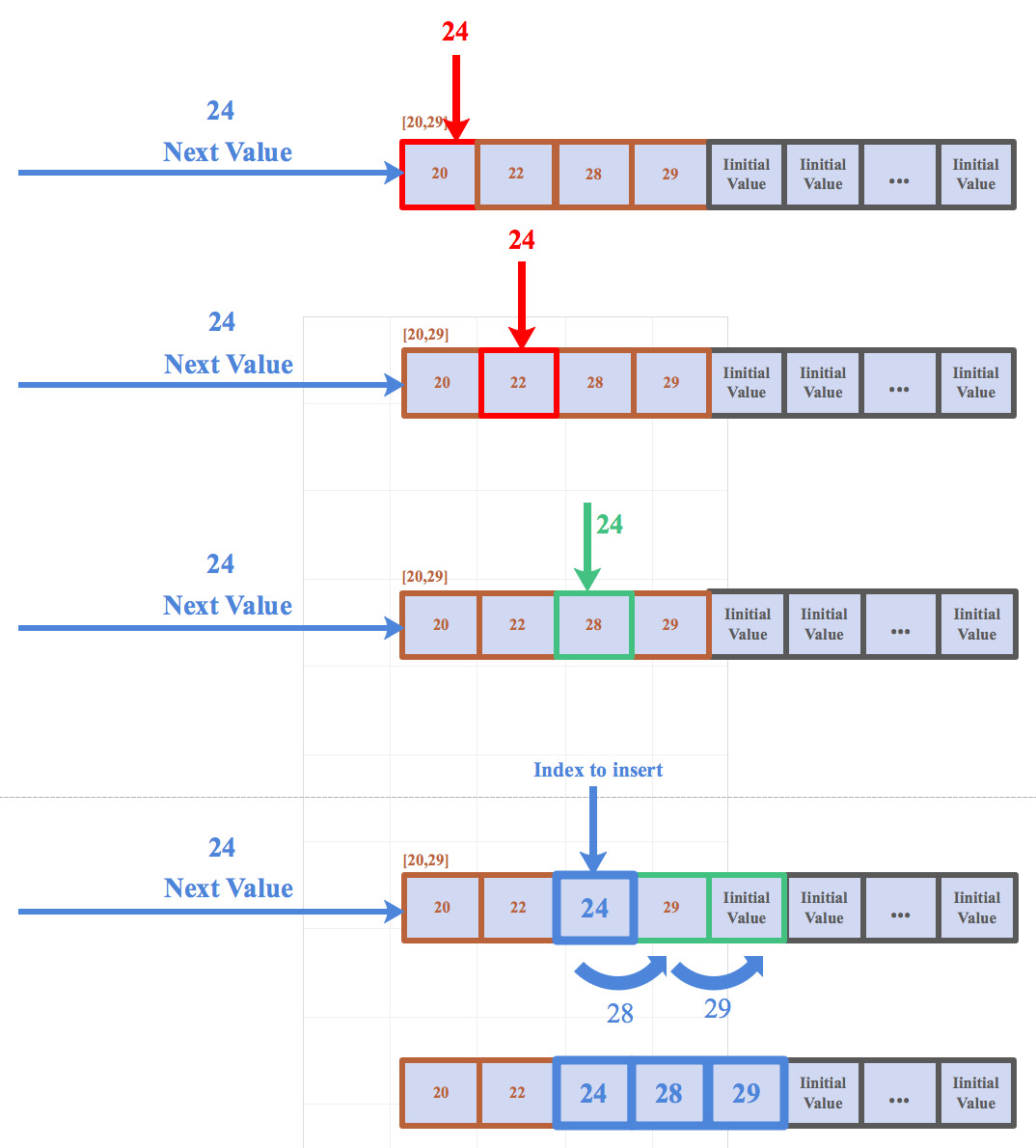
This way, the segment holds either a single Run or parts of two Runs at any given point. In the latter case, the older Run shrinks while the younger one grows respectively. When the last value in the older Run is removed, the older Run no longer occupies any space in the switch. At this point, the younger Run becomes the older Run and the next incoming value creates a new younger Run. In more details, we distinguish between the following cases:

Case 1:

The segment is empty, meaning that the value is stored in the first stage.

Case 2:

The segment is not empty, but not full either. Here, the new value is compared to the values that are already stored in the pipeline (when the pipeline is not full, the first stages are populated). For each stage, if the current value is bigger or equal to the value in the current stage, we continue to the next stage. If the current value is smaller than the current stage, then the current value and current stage are swapped. In this case, the new current value is passed to the next stage, and they are also swapped. This process is repeated for each stage, until there is an empty stage, and the last current value is stored in that stage. If the current value is bigger or equal to the value in the last populated stage, it is stored in the first available stage. See illustration in Figure 9.

Case 3:

The segment is full. The first time this happens, all the values inside the segment are ordered in ascending order and constitute a Run. The smallest value is moved to the output, and the new current value substitutes it, creating a new Run. Now there are two Runs in this segment. In fact, the latter happens each time there is a single Run in the segment (which happens every segment length arrivals).

If there are two Runs, the smallest value in the older Run is removed. That is, the first index of the older Run becomes available and assigned to be the last available index of the younger Run. Now the new current value is inserted to the younger Run in the same way as in case 1 with respect to the last new index of the younger Run. The new first index of the old Run is forwarded to the next stage. When the old Run is empty, the younger Run becomes the older Run and the first index of the older Run is the first index of the previous younger Run, which is also the first index of the pipeline. See illustration in Figure 10.

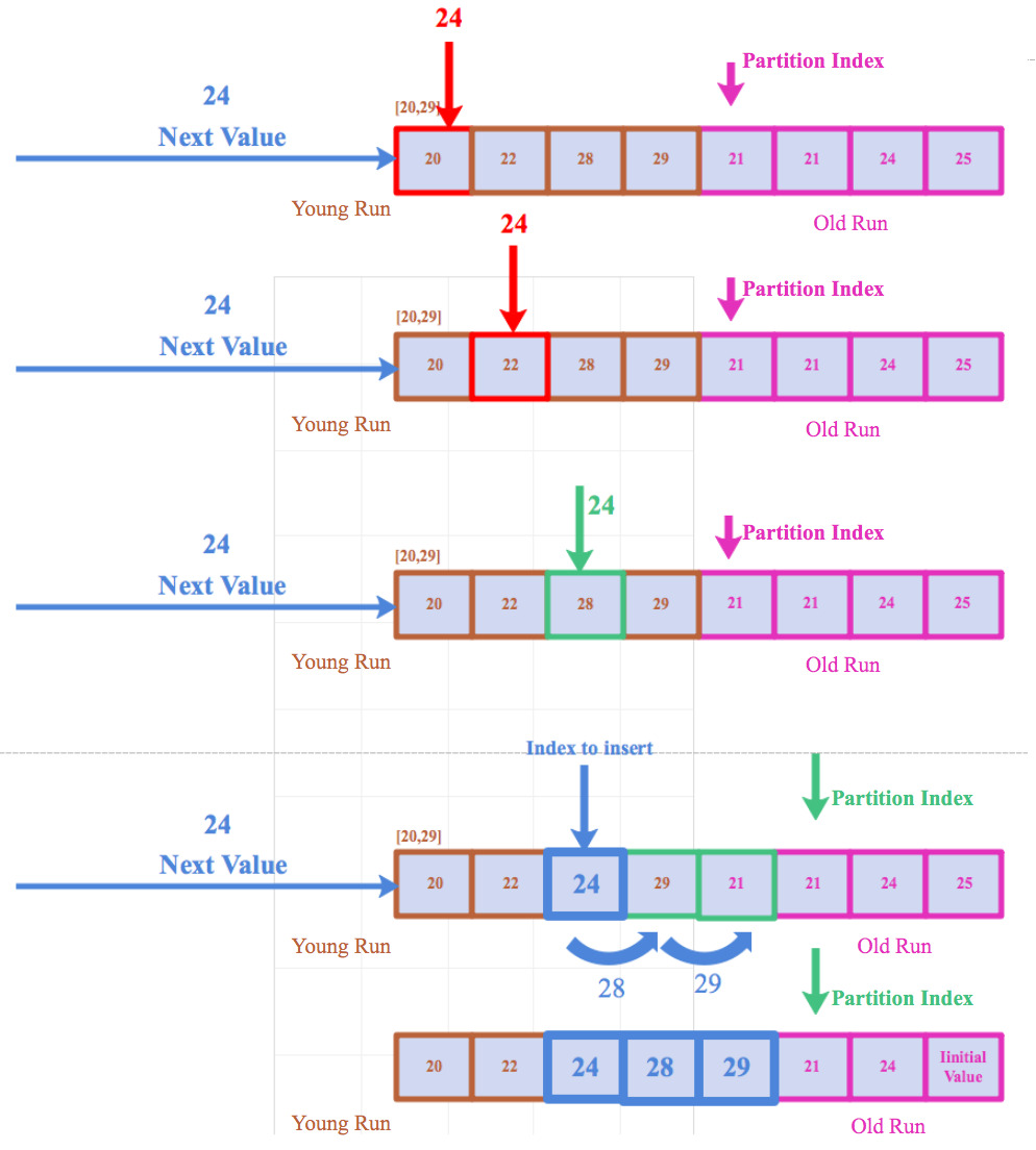
Each value is emitted with its matching segment number. When there are no more lines to read, the switch does a flush action and outputs the remaining values. It first does one pass and flushes out the older Run. Then, it performs a second pass and flushes out the younger Run (if exists).

The server receives the values and their segments. It invokes the merge sort algorithm on each segment separately (every two values in two different segments are strangers). After each segment is sorted, the server unites the segments according to their serial number, and then outputs all the values into one output. The final output is the sorted values in ascending order.

The number of segments and their length are part of the architecture of the switch. In our work it is a parameter, in order to explore the impact of this design choice on the performance of the overall sorting task. The maximum value is needed only for the ranges calculation at initialization.

To set the ranges, the algorithm executes one division action and saves the remainder. The programmable switch cannot perform a division in the RMT model. This can be solved in several ways: The results can be calculated at the server before the beginning of the execution and then dictated to the switch. They can also be received as a parameter, or they can be calculated by approximation of division with TCAM and log operations [19]. This is feasible because the division is done only once at the beginning.

Finding the right segment for an item can occur at the parsing stage, before the algorithm starts.

This part is the heart of the algorithm. When a packet arrives, it is parsed and traverses through the pipeline stages as part of the routing process. The value that is parsed is compared each time with the value in the current stage. Comparison is a simple action that is allowed.

In each stage, when the packet arrives, a comparison is performed. If needed, the value in the packet swaps with the value in the stage. The bubbling of the values forward is performed by placing this value in the packet. In particular, to swap values, the value in the stage is swapped with the one in the packet, and then the packet moves on to the next stage.

The output value is saved in the packet when we first identify it. It is output with the segment’s number as a port number, and thus the server can identify the segment. We notice that each stage has its own memory and there is no branching or access to memory of any other pipeline stage. Also, this requires only a small amount of memory.

Since the packets are processed in parallel, and each stage in the pipeline processes another packet, we cannot afford a partition index that is implemented by shared memory. This is overcome by a dedicated variable that signals whether the stage is the partition index or not. This variable counts each packet that passes through the stage. From the algorithm’s structure, after the first $segment\_length$ iterations, the $i^{th}$ stage becomes the partition index every time the iteration counter modulo $segment\_length$ equals to $i$ (when the counting of the stages and iterations starts from 0). It is enough that each stage detects if it is the partition index itself, because the comparison and swapping are performed locally in the stage. When a packet traverses through the pipeline, it can be swapped with the stages until it passes the partition index stage. When it arrives to the partition stage, it is marked, so the next stages can notice that this packet must not be swapped anymore.

In the first segment length iterations, there are still empty stages (with the initial value). According to our algorithm, each stage can maintain a Boolean flag bit to mark stages with the initial value. When a packet passes through an initial value stage, its value can be stored in that stage.

All the processing can be done in parallel, packet by packet. Each stage can process its temporal packet because each stage knows its value and the current packet value, so the unit can perform a comparison.

After the input stream ends, the pipeline stages are still full with values. To emit these values while preserving their order, we perform a flush action. The Flush can be done by a particular packet that passes through the pipeline and collects the values in their order at the switch. The flush can be finished in two rounds using the recirculation mechanism of P4: In the first round, the packets of the old Run are flushed while items belonging to the young Run are ignored (to continue the sequence). In the second round, it flushes out the younger Run.

We present the results in 3D graphs. In Figure 12 we exhibit the random trace results. Figure 13 shows the network trace results and Figure 14 represents the results for the memory trace. The graphs are similar in their trends, which fit the theoretical analysis. We can also see that the improvement comes from both the parallelism and the number of stages, and even when only one of them increases and the other one stays fixed, the run-time become shorter.

In Figure 15, we can see an example of the random average graph, with a line that separates between the time reduction trends. Above the line, when the number of segments and the segments length is under 16, the improvement in the run-time is more significant than under the line, which implies that there are values for number of segments and segments length that satisfy the design trade-off explained in Chapter 3. If these values are between the range $(8,16)$, we achieve a significant improvement compared to the original run-time without MergeMarathon. Beyond these levels, the returns diminish very quickly.

To understand better the influence of each parameter about the run-time, we present 2D graphs of average and median time. There are two types of graphs: In the first type, we fixed the segment length, and examined the run-time reduction as a function of the number of segments. In the second type, we fixed the number of segments, and examined the run-time reduction as a function of the segment length.

In Figures 16, 17 and 18 we exhibit the 2D graphs of the average and the median run-time in seconds for the random trace with MergeMarathon. In each Figure, Graphs (a) and (c) represent the time reduction vs. the number of segments and the different colors represent the different segment lengths. Graphs (b) and (d) represent the time reduction as a function of the segment length and the different colors represent the different numbers of segments. We analyze the graphs and their trends.